Abstract
In recent times, studies about the accuracy of algorithms to predict different aspects of energy use in the building sector have flourished, being energy poverty one of the issues that has received considerable critical attention. Previous studies in this field have characterized it using different indicators, but they have failed to develop instruments to predict the risk of low-income households falling into energy poverty. This research explores the way in which six regression algorithms can accurately forecast the risk of energy poverty by means of the fuel poverty potential risk index. Using data from the national survey of socioeconomic conditions of Chilean households and generating data for different typologies of social dwellings (e.g., form ratio or roof surface area), this study simulated 38,880 cases and compared the accuracy of six algorithms. Multilayer perceptron, M5P and support vector regression delivered the best accuracy, with correlation coefficients over 99.5%. In terms of computing time, M5P outperforms the rest. Although these results suggest that energy poverty can be accurately predicted using simulated data, it remains necessary to test the algorithms against real data. These results can be useful in devising policies to tackle energy poverty in advance.
1. Introduction
1.1. Energy Poverty: Definition and Conceptualization
Energy poverty, also called fuel poverty or energy vulnerability, takes place when households cannot keep comfortable temperatures inside their homes or cannot access energy services at a reasonable cost [1,2]. This phenomenon has received the attention of the scientific community and society in recent years due to its political and social implications [3,4]. Previous research has shown that energy poverty is a driver for the physical deterioration of residents [5,6] and is even responsible for a higher death rate in winter due to the poor thermal conditions inside buildings [7,8]. There is a wide consensus about the fact that energy poverty stems from a combination of high-energy prices, low family income, inefficient buildings, and outdated electrical household appliances [9,10]. Additionally, occupant behavior can contribute to new cases of energy poverty [11,12].
The measurement of energy poverty is a challenge because its condition is culturally sensitive and private, as well as temporal and dynamic [2]. It is a relative concept influenced by different variables, whose importance may vary depending on the context [13]. The limited availability of data and indicators, together with a lack of consensus on how energy poverty should be conceptualized and measured, makes the matter even worse. Energy poverty indicators are thus a pressing need in this research and political landscape [14]. The United Kingdom pioneered the study of fuel poverty in 1991, with the publication of the seminal work by Boardman [15] that later spread across other European countries. Nowadays, several European countries, such as Slovakia, France and Ireland, have conceptualized fuel poverty building upon a multidimensional approach based on indicators [16]. Those can be divided into six categories: (i) indicators based on the relationship between household income and expenses [17,18]; (ii) multidimensional indicators [19,20]; (iii) indicators based on self-reported housing condition [21]; (iv) indicators of econometric analysis [22,23]; (v) indicators associated with the energy rating of dwellings [24,25]; and (vi) indicators calculated according to the thermal comfort [26]. From a wider perspective, energy poverty includes other factors, such as social exclusion [5] and the limited availability of some energy sources [19]. Outside Europe, fuel poverty has been addressed mainly from the economic perspective, that is, as a balance between household income and expenses. Nevertheless, in countries like Japan, more recent attention has focused on the multiple facets of fuel poverty [27]
A considerable amount of literature has been published on fuel poverty in developed countries, but the existing accounts fail to describe the situation in underdeveloped or developing countries. In this regard, Chile’s current situation is worth to be noted for two reasons: First, the country has continuously implanted, since the mid-20th century, a strong policy on social housing, providing the vulnerable strata of society with affordable dwellings; as per the last census of 2016, around one million and a half dwellings have been completed [28]. On the contrary, the geography of the country gives a very particular energy market; Chile has one of the highest prices of electricity among the member countries of the OECD [29]. Despite being a member of this organization since 2011, the gap between the richest and poorer strata of society is still evident. Previous research has shown that a considerable number of families face difficulties in paying the energy to keep their homes comfortable [30], and many others cannot adequately ventilate or heat them up [31]. According to a recent report by the Chilean government, 20% of the homes do not have hot water, and the indoor temperature in summer and winter is not acceptable in 76% of the surveyed homes [30]. A study conducted by the Chilean Chamber of Construction has presented the breakdown of the energy use of Chilean households: 56% is allocated for keeping their homes within acceptable thermal conditions, 18% for hot water, and 26% for electrical appliances [29].
These circumstances compelled the Chilean government to take action. In 2014 the Chilean Ministry of Energy presented the Energy Agenda, whose main tasks was the design and execution of a long-term Energy Policy for 2050 [32], which builds upon four aspects: (i) security and quality in the supply chain, (ii) energy as a driver for the development of the country, (iii) compatibility with the environment, and (iv) energy efficiency and education. Within the second aspect, one of the lineaments was the conceptualization and measurement of energy poverty to establish specific policies towards it. The objective is to reduce energy poverty levels by 50% by 2035 and by 100% by 2050 [33]. As previously mentioned, owing to the fact that measuring energy poverty strongly depends on the culture, climate, and socioeconomic conditions of each country [34], the government of Chile signed an agreement with The United Nations Development Program to elaborate a conceptual and methodological framework specifically designed for Chile [35].
1.2. Energy Poverty in Chile
Over the past decade, the conceptualization of energy poverty has progressed in Chile, but much of the research has exclusively focused on identifying this issue ex-post. However, there has been little discussion on how energy poverty can be predicted in advance thus far; that is before a family moves into a new house with new heating and cooling systems, electrical appliances and energy consumption. Understanding this research gap, the authors took the lead and started a new line of research that offered some important insights into the importance of predicting energy poverty in advance [31,36,37]. Evidence for these studies suggests that two main factors should be considered: The household income and the adopted comfort model; both of them are introduced below.
According to the Chilean national socioeconomic survey, Chilean families can be divided into 10 different groups (called deciles) depending on their income. The 10th decile corresponds to the wealthiest families and the 1st decile to the poorest. Table 1 indicates the ranges of the mean monthly income corresponding to each decile in 2006, 2009, 2011, and 2013.

Table 1.
Variation of ranges of Chilean deciles in recent years [38].
Second, the energy expenditure of households can be modeled according to the gap between the indoor and outdoor temperature. In this regard, a much-debated question is whether to use a static or an adaptive thermal comfort model. The static comfort model, which is adopted by many national standards, considers static setpoint temperatures. However, it fails to explain people’s ability to adapt themselves to the thermal variations inside their homes within certain limits. Current Chilean standards use this approach (Table 2).
Table 2.
Comfort limits indicated in the sustainable construction standards for housing in Chile.
The adaptive comfort model builds upon the fact that inhabitants can adapt to thermal variations taking certain actions: Adapting their clothing and ventilating the building. These adaptive measures are feasible when indoor temperature, which is a function of the outdoor thermal variations [39], is within a certain range. Previous research has shown that adaptive thermal models can better represent the real energy consumption of buildings, which can vary between 10% and 18% when compared with the theoretical approach of the static model [40].
Since evidence suggests that the adaptive comfort model can better explain the real energy consumption of buildings, the authors have recently examined the influence of the application of such a model on the quantification of energy poverty and have developed a new index called the fuel poverty potential risk index (FPPRI). The theoretical basis is detailed in previous publications by the authors [41] and also has been tested against different scenarios of climate change in Chile [42], also using advanced simulation techniques, such as multiple linear regression [37].
Evidence from these previous studies suggests that these techniques can predict the risk of fuel poverty with acceptable accuracy, but it still remains unknown whether other advanced techniques may outperform the former. There is still uncertainty whether fuel poverty can be predicted with different regression algorithms. The specific objective of this study is to test the accuracy of six regression algorithms to predict the risk of fuel poverty, expressed by the FPPRI (i) multilayer perceptron (MLP); (ii) -nearest neighbors (-NN); (iii) classification and regression tree (CART); (iv) random forest (RF); (v) M5P; and (vi) support vector regression (SVR). These algorithms were chosen because they are commonly used in the prediction of energy consumption in the building industry, as pointed out by a recent study [43], which concluded that interplay between the architecture of the models and the predicted phenomenon exerted a strong influence on the final accuracy. Debate continues about, which is the algorithm that best-fits each problem, and therefore this exploratory study aims to unravel the accuracy of these six advanced regression techniques in predicting the risk of falling into fuel poverty of financially deprived households in Chile by means of the FPPRI index.
It is expected that this research will contribute to a better understanding of how to predict energy poverty in advance, therefore making it possible to detect and tackle the problem in a swift and effective way. This new understanding should help designers and policymakers in building and delivering affordable and efficient social dwellings and in allocating financially deprived families in new houses whose energy expenditure would be suitable for their income level.
This paper is organized in the following way: First, an explanation of the predictive models is provided. Second, the predictor variables for the models are determined, and afterward, the data processing and results are presented. Finally, the results obtained by all models are compared and evaluated, which leads to the discussion of results and conclusions on the feasibility of such models.
2. Materials and Methods
2.1. Regression Algorithms
As previously mentioned, six regression algorithms were considered in this study. For each one of them, a brief explanation of its architecture and its main characteristics is provided. This information will be used later on to discuss the results of each one of them.
2.1.1. Multilayer Perceptron
A neural network is a statistical model simulating the neurological brain structure to solve linear and nonlinear problems [44]. This model is a computation paradigm, which allows complex problems, both classification [45,46] and regression problems [47,48], to be tackled. Neural networks have been widely used in the field of energy analysis over the last years: (i) Deb et al. [49] developed a neural network model to predict the energy saving associated with HVAC in office buildings and compared the results to multiple linear regression. The results determined a better performance for the neural network than linear regression, with a correlation coefficient higher than 37.25%; (ii) in a later study also by Deb et al. [50], a model was developed to predict the cooling load of the next day using data of the previous five days. The methodology showed an adequate accuracy, with a correlation higher than 94% in the days analyzed; (iii) Magalhães et al. [51] developed an artificial neural network model to predict the heating energy demand based on the occupants’ behavior. The results obtained models with a correlation coefficient higher than 93%; (iv) Kljajic et al. [52] developed a neural network to predict the efficiency of boilers according to the operating performance as well as to predict possible improvement measures; and (v) Kialashaki and Reisel [53] conducted a large-scale application of the algorithm, designing a model to estimate the energy demand in the residential sector of the United States using historical data from the last years.
From the various architectures of artificial neural networks, MLPs are those providing the best features because they are supervised models with universal approximation capacities [54,55]. The MLPs are characterized by presenting an architecture of three or more layers (see Figure 1): an input layer, one or several intermediate layers, and an output layer. There are a series of nodes in each layer. The output value of each neuron is obtained by the sum of values of the input neurons weighted by synaptic weights and by applying an activation function (Equation (1)). These connections spread to the output layer (Equation (2)), obtaining the model’s response ().
where are the values of the input layer, and are the weight and the input value of the bias neuron of the input layer, respectively, are the weights of the hidden layer, and are the weight and the input value of the bias neuron of the hidden layer, respectively, are the weights of the output layer, is the output of a neuron of the hidden layer, and is the activation function. For this study, a sigmoidal activation function was used both in the hidden and the output layer (Equation (3)). The advantage of this kind of function is the possibility of comprising an infinite input set into a finite output set.
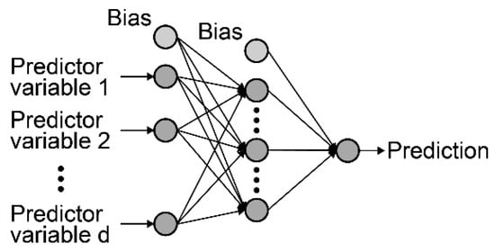
Figure 1.
Scheme of a multilayer perceptron (MLP) model.
The main objective of the algorithm is the adjustment of synaptic weights guaranteeing that the predicted output value for each input vector is near to the actual output value. For this purpose, a learning algorithm is applied to a training dataset. The models were trained by backpropagation [56], using the Broyden–Fletcher–Goldfarb–Shanno (BFGS) algorithm [57], which belongs to the set of quasi-Newton methods. The number of nodes and the number of hidden layers is analyzed to determine the best model [47]. For this study, architectures of 1 hidden layer were considered because they had better performance than more complex structures [58], but the number of nodes in such layer was analyzed.
2.1.2. K-Nearest Neighbors
The -NN algorithm (also known as instance-based learning with parameter ) classifies observations based on the majority class between the nearest observations [59]. These observations, or neighbors, are chosen from the training dataset in which the classification value is known. The -NN algorithm is used for class label problems [60] and regression analysis [61], implying their use in the energy analysis of installations and buildings: (i) Ramakrishna Madeti and Singh [62] developed a -NN model to detect failures in photovoltaic devices. The percentage of instances correctly classified by this model was higher than 98%, obtaining better performance than other existing models; (ii) Rodger [63] developed a -NN model to predict the heating energy demand. The values predicted by the model presented a correlation higher than 94% with respect to the actual values; and (iii) a model to determine the number of occupants inside the building during the monitoring was used [64]. The results obtained by the model designed in this study presented a higher accuracy that those obtained by linear discriminant functions.
In the regression analysis, the -NN algorithm determines the value of the observation analyzed as an average of the nearest neighbors’ values () of the training dataset. To determine the closeness between observations, a metric distance is used. This distance strongly affects the performance of the model [65], so it is necessary to study which distance presents a better performance in the model. In the present study, the Minkowski distance was used (Equation (4)). This distance is characterized by the fact that the Minkowski distance is equal to other metric distances depending on the value assigned to [66]: (i) the Manhattan distance ( equal to 1); (ii) the Euclidean distance ( equal to 2); and (iii) the Chebyshev distance (when is near to the positive infinity). After determining the distances, the output value of the model is given by Equation (5). The output value () is obtained as the average of values () of the nearest points. As can be seen, is a key parameter in the model’s response [67]. Both and were therefore analyzed due to their influence on the performance of the model.
2.1.3. Classification and Regression Tree
The CART algorithm, developed by Breiman et al. [68], constructs models in a reverse tree shape. Such models divide the input space into subregions, simplifying complex with simple problems [69]. Trees are composed of internal nodes corresponding to variables, arches to values of the root node, and leaves to the value of the dependent variable. Trees are easy to interpret because a scheme of nodes and leaves is available, thus easing the understanding of the solution adopted for the problem [70]. For this reason, trees are used in several works: (i) Tso and Yau [71] developed models to predict energy consumption by using three different algorithms: CART, MLP, and linear regression. The results revealed that both the CART and the MLP model obtained better performance than the linear regression; (ii) Mousa et al. [72] analyzed the use of a CART model to estimate the air change rate in buildings; and (iii) in another study [73], a CART model was developed to predict the monthly energy consumption in residential buildings. The results showed that the tree model obtained better performance than linear regression and multivariate adaptive regression splines.
The optimal structure is obtained by the binary recursive partitioning process during the development of the model: each node of the model has a partitioning rule. This rule is established by decreasing the total residual sum square. After carrying out the induction, the application of the pruning (that is, the removal of the inefficient nodes) allows the complexity of the model to be generalized and reduced [74]. The depth of the tree and the minimum number of instances per node is needed to be established in the configuration of the algorithm. These parameters affect the complexity and performance of the model, so they were analyzed.
2.1.4. Random Forest
As indicated above, the simplicity and interpretation of CART models make their use easier. However, many studies reflect the limitations of such models [75,76]. RF allows a solution to these problems to be adopted by creating a set of CART models generated in parallel to reduce the variance and the bias of the RF model [77,78]. RF is an ensemble learning algorithm, which obtains a better behavior than an individual model [79]. Another advantage of RF is the possibility of using large datasets, as well as not being affected by atypical values [80]. This aspect allows this model to be used to predict energy consumption. In this sense, Li et al. [81] developed an RF model to predict the daily electricity consumption in companies. The model had a more accurate prediction than artificial neural networks and support vector machines. Likewise, its monthly [82] and hourly [83] use as a predictive control system of HVAC systems has been analyzed in some studies.
For the RF training, bootstrapped sample sets are drawn from the training dataset [78]. Each bootstrapped sample allows a forest regression tree to be generated. Moreover, each node of each tree is divided using a subset of predictors m randomly selected. This reduces the influence of the strongest predictors. After generating the set of -trees and following the RF model structure (see Figure 2), the regression estimator () is as follows:
where is the number of trees, and is the output of the -th tree.
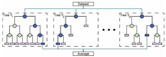
Figure 2.
Scheme of a random forest (RF) model.
The number of trees used by the model influences its performance [84]. For this reason, different numbers of trees were analyzed to obtain the model with the most efficient behavior.
2.1.5. M5P
The M5P algorithm (also known as M5) is an evolution of the CART algorithm [85,86]. Unlike the CART model, M5P combines decision trees with multiple regression: a decision tree is constructed following the same structure of reverse tree from the CART model, but a multiple linear regression (MLR) model is adjusted in each leaf of the model (Equation (7)). The algorithm, therefore, develops an MLR model in each subregion. In the development of the M5P tree, the internal variation of subsets for the class values of each branch is minimized instead of maximizing the information gain. After constructing the model, the pruning allows the overfitting to be reduced. The advantages of the models generated by this algorithm are the efficient use of huge amounts of numeric variables and their robustness because of the lack of values in the instances of the dataset analyzed [87,88]. The use of this model for the energy characterization of buildings has therefore increased in recent years. In this sense, Li et al. Afsarian et al. [89] developed an M5P model to predict the total energy consumption in a reference building. The results obtained a greater than 90% in most datasets. In another study by Jeffrey Kuo et al. [90], a comparative study of regression models was conducted to estimate the energy consumption in convenience stores of Taiwan. The use of four different models (M5P, Gaussian processes, linear regression, and support vector regression) was compared. The results obtained by M5P obtained a more accurate estimation than the other models. Likewise, M5P has a good performance in determining oscillations in energy prices. In a study by Azofra et al. [91], a model was developed to determine the variations of the cost of electricity tariffs because of the generation of photovoltaic and wind power in Spain. The model was used to analyze various scenarios, thus determining the possible saving in the cost of electricity tariff.
where is the independent term, are the regression coefficients, are the predictor variables, and is the error.
2.1.6. Support Vector Regression
SVR is an application for regression analysis of the support vector machines [92]. SVR consists of transforming the root input variable in the space of higher dimension where two classes are separated by an optimal hyperplane [93,94]. Some advantages of SVR are the facts that they are less subject to overfitting [95] and their good behavior when tackling nonlinear problems [96]. It is an algorithm widely developed in the energy control of installations, such as lighting [97] and HVAC systems [98]. Likewise, SVR has been used in some studies to estimate the energy consumption in residential buildings [99,100] and offices [101,102].
For their mathematical approach, support vector machines approach the relationship between the output and input parameters by using the following equation:
where is representative of a nonlinear mapping function, is a weight vector, and is the bias term. and can be predicted by minimizing the regularized risk function (Equation (9)), guaranteeing the restrictions of Equation (10).
where is the sampling number, is penalty parameter to control the compensation between the regularization term () and the training error, is the maximum error allowed, and represent the distance of the actual values from the upper and lower limit of the error allowed, respectively.
Finally, the output of the SVR (Equation (11)) is obtained by introducing Lagrange multipliers ( and ) and a Kernel function (). In this regard, it is essential to determine which kernel function is used. There are different kernel functions: linear, polynomial, sigmoidal, and radial basis function (RBF). For this study, the RBF kernel is used (Equation (12)) because models with the best performance are obtained, and a lower number of parameters should be considered to improve the behavior of the model [74,103].
The parameters that should be considered to improve the performance of the model are and . To determine the model with the best performance, different combinations of and were used.
2.2. Dataset and Model Construction
2.2.1. Description of the Dataset
Based on the calculation methodology by Pérez-Fargallo et al. [31,36], the procedure to determine the dataset was described in a previous study [37]. The case studies were configured using different parameters of the A1 and B1 typology of the social dwelling of the Chilean Ministry of Housing and Urbanism (MINVU in Spanish) [104]. A total of 7776 case studies were configured. Likewise, each case study is considered to belong to each of the 5 poorest deciles [105]. Thus, 5 different datasets per decile, composed of 7776 instances, were obtained. In total, 38,880 cases were considered.
The predictor variables were as follows: (i) orientation (OR), (ii) form ratio (FR), (iii) volume (V), (iv) surface in contact with the ground (SG), (v) horizontal surface area in contact with another dwelling (SH), (vi) roof surface area (SR), (vii) vertical surface area in contact with another dwelling (SV), (viii) shadow distance (D), (ix) shadow height (H), (x) energy price (EP), and (xi) income (IN). Figure 3 shows Pearson’s correlation coefficients and the p-values. For nearly all of them, the null hypothesis can be rejected, and the Pearson’s coefficient shows no evident correlation. A more surprising correlation is found between the group of variables related to the design of the dwelling (SG, SR, SH, SV and V), for, which the null hypothesis cannot be rejected, and moderate correlations are found in some cases. This is because those are interweaved in the design of the dwelling, but this does not compromise the accuracy of the model. The dependent variable was the FPPRI, which was logarithmically transformed to improve the accuracy of the final model.
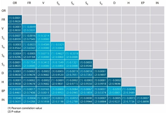
Figure 3.
Pearson’s correlation values and -values between predictor variables. The significance level of the p-values was 0.05.
2.2.2. Training and Validation Procedure
As indicated above, five datasets containing 7776 instances were obtained per decile. Likewise, a full dataset with the case studies of the five deciles was generated (38,880 observations). These datasets were used to generate 6 different models for each regression algorithm: one per each decile (D1, D2, D3, D4, and D5) and another per all deciles (T). The datasets were randomly divided into two sets: 75% of the observations corresponded to the training dataset, and the remaining 25% to the testing dataset.
For the models’ training, a 10-fold cross-validation was carried out. Cross-validation allows the bias and the variance of the model to be reduced [106]. All training datasets were randomly divided into 10 subsets. For each fold, 9 subsets were used for the training, and the remaining for the testing (Figure 4). The performance of the model is obtained by the average value of the 10-fold.
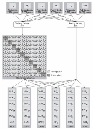
Figure 4.
Flowchart of the training and testing.
Three statistical parameters were used to evaluate the performance of the models: (i) the correlation coefficient () (Equation (13)), the root mean square error () (Equation (14)), and the mean absolute error () (Equation (15)). The use of these parameters allows the performance of the models to be correctly defined [107] and also are amongst the most used when comparing the performance of algorithms with different architecture [43]. The lower the value of and , the greater the accuracy. The threshold value of R2 was set at 0.95 to consider the predictions sufficiently accurate [37,48].
where is the model’s prediction, is the actual value, and is the number of instances in the dataset.
3. Results and Discussion
This section is organized as follows: First, the results from each algorithm are presented, along with a discussion of the particular features of their architecture. Finally, all algorithms are compared on the basis of the three parameters: R2, MAE, and RMSE.
3.1. Performance of the Models
3.1.1. MLP Models
The performance of the MLPs model was analyzed on the basis of the number of neurons in the hidden layer. As mentioned in Section 2.1, only one hidden layer was considered because it usually delivers better performance than more complex architectures [58]. Table 3 indicates the optimal number of neurons obtained for each model and the performance obtained in both the training and testing phases. What stands out in this table is that the optimal number of neurons in the hidden layer was very similar between the different models (between 12 and 14 nodes). Regarding the accuracy, was greater than 99.8% for all models in the training and testing phases, was lower than 0.010, and lower than 0.012. The accuracy did not vary when considering the full dataset or each decile separately.
Table 3.
Results of training and testing of the MLP models.
3.1.2. K-NN Models
For -NN models, two parameters, and , have an influence on its accuracy. In this case, values of ranged between 1 and 25, and values of between 1 and 4 (Figure 5). A different behavior was observed depending on the type of dataset used: for models per deciles, a value of of 2 (corresponding to the Euclidean distance) obtained the best performance, whereas, for -NNT, a value of of 4 obtained the best statistical parameters. In this regard, the number of close instances used by the model varied: for models per deciles, values of between 9 and 11 obtained acceptable results (in the testing, was between 0.059 and 0.072, and between 0.076 and 0.094), whereas, for -NNT, the number of was 2. The performance of -NNT was lower than models per deciles because a low number of instances was used to obtain a representative result (in the testing, was 0.082 and was 0.110). In this sense, both in the training and testing phases, was always below 0.95, except for one case, and were very similar for all sets of data (Table 4).
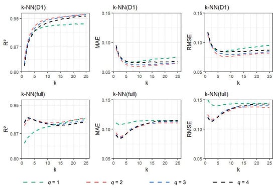
Figure 5.
Values of , , and obtained for and .
Table 4.
Results of training and testing of the -nearest neighbors (-NN) models.
3.1.3. CART Models
In this model, the parameters of depth and instances per node were analyzed: the depth of the tree oscillated between 2 and 12 (the maximum value was established according to the number of variables of the dataset), and the number of observations per node ranged between 2 and 30. Figure 6 is a sample of the analysis carried out. The performance of the model is strongly influenced by the depth of the tree: the higher the depth, the greater the correlation (values of greater than 97.80%) and the lower the MAE and RMSE. The most optimal depth for all models was, therefore, the maximum suggested (12 levels). Although this could mean overfitting to training data, the performance obtained in the testing phase was similar to that obtained in training (Table 5); therefore, it was not considered necessary to generalize the tree (i.e., to simplify it) to obtain a better performance in new observations. When comparing the accuracy for the full dataset and for each decile, the full model (CARTT) delivered better results than each decile separately in the testing phase. increased between 1.0 and 1.3%, and and had values lower than 0.008 and 0.010, respectively. This is because the structure obtained is better adjusted to the full dataset than to the models per deciles.
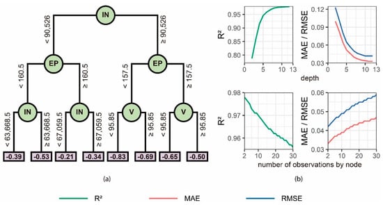
Figure 6.
Training of the classification and regression tree (CART)D1 model: (a) scheme of the CART model for a depth of 3; and (b) statistical parameters both of different values of depth and the number of observations by node.
Table 5.
Results of training and testing of the CART models.
3.1.4. RF Models
In this model, the number of trees influences the performance of the model. For this reason, the behavior of the model with a number of trees between 1 and 200 was analyzed by using both the same depth and number of instances used in the CART models. Figure 7 represents the performance obtained for the RFD1 model, whereas Table 6 indicates the values obtained for all models. As can be seen in Figure 7, the performance of the model improved as the number of trees increased. However, when the optimal value was reached (149 in the case of D1), the performance of the model did not improve: the number of trees only increased the time required to train the model. Likewise, the optimal number obtained for each model was very similar, varying between 143 and 153. With respect to the models obtained, the performance was very similar for models per deciles and the full model. In this sense, obtained values between 99.3 and 99.6%, whereas and oscillated between 0.021 and 0.023 and between 0.027 and 0.030, respectively.
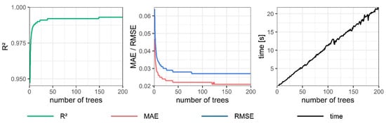
Figure 7.
Influence of the number of trees on the behavior of RFD1.
Table 6.
Results of training and testing of the RF models.
3.1.5. M5P Models
In M5P models, no parameter was analyzed to optimize their performance. As can be seen in Figure 8, M5P determines the optimal depth of the model. Therefore, it is not necessary to analyze this aspect in such performances. Regarding the values of the statistical parameters, the performance was very similar (Table 7): was between 0.995 and 0.998, between 0.014 and 0.016, and between 0.018 and 0.020.
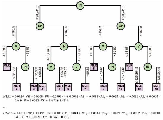
Figure 8.
Structure of the M5PD1 model.
Table 7.
Results of training and testing of the M5P models.
3.1.6. SVR Models
As indicated in Section 2.1.6, both and affect the performance of the SVR models. Different combinations of these two parameters were therefore analyzed. In this sense, adopted values between 0.1 and 4, whereas was analyzed using values between 0.05 and 0.2. Figure 9 represents the results of the various combinations in SVRD1, and Table 8 indicates the optimal configuration and the results obtained by each model. Several aspects can be appreciated from the analysis: (i) optimal values of the models were obtained from values of of 0.15. Although best values in the statistical parameters were obtained as the value of increased, the value of obtained the same values for lower values of . Values lower than 0.15 did not obtain the same optimal performance; (ii) high values of and influenced the training time. In this regard, the time difference between different values of was greater than 1000 s, slowing down the training with high . Thus, the optimal value of obtained for all models was 0.15, whereas the value of varied between 1.6 and 2.1 (Table 8). Likewise, the performance obtained both in the training and testing phases was similar. SVRT presents quite similar to models per deciles in the testing, is greater than 0.002, and ranges between 0.004 and 0.006.
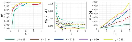
Figure 9.
Influence of and on the behavior of SVRD1. Values of are represented by the discontinuous line.
Table 8.
Results of training and testing of the support vector regression (SVR) models.
3.2. Comparison of Models
The algorithms were compared on the basis of two parameters: (I) the individual performance obtained by each decile and (ii) the performance obtained in the estimation of the 5 deciles together. Figure 10 shows the scatter plots comparing the actual and predicted values of the total dataset (as well as the values of the statistical parameters), and Table 9 is a compilation of the statistical parameters obtained per deciles separately. Likewise, the point obtained by each model per decile is represented in Appendix A (Figure A1, Figure A2, Figure A3, Figure A4, Figure A5 and Figure A6). Several aspects regarding the comparative analysis are worth noting. First, the estimation conducted by each model was merged in a combined estimation (D1–5) with the corresponding values of , , and . Then, the full model of each algorithm was used to evaluate the estimation conducted in each decile.
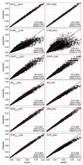
Figure 10.
Comparison of actual and predicted values obtained by each model. The testing dataset used is indicated in brackets.
Table 9.
Statistical parameters were obtained by each regression algorithm in the testing phase per each decile.
Regarding the performance obtained by each decile, there were different results. The algorithm that delivered with the worst performance was -NN: was lower than 95% for almost all decile models (only D1 obtained of 95%), whereas -NNT had a different behavior depending on the decile analyzed, obtaining the best behavior in deciles 3, 4, and 5, and the worst in deciles 1 and 2 (0.880 and 0.939). Therefore, the performance obtained using the -NN algorithm was not considered adequate (see Figure 10).
The use of the other algorithms gave optimal correlation coefficients (higher than 98% in all cases). The analysis of the error parameters revealed that CART and RF models obtained error values higher than MLP, M5P, and SVR: and increased regarding the highest value of M5P of 21.43% and 23.53%, respectively. Therefore, the performance obtained by these two models, although being acceptable, did not present the adjustment degree of MLP, M5P, and SVR. Regarding these three algorithms, the results were quite similar for all the cases analyzed: oscillated between 0.996 and 0.999, between 0.008 and 0.018, and between 0.010 and 0.026. Despite the performance obtained by the full models in each decile was optimal, SVRT had the worst performance in deciles 1 and 2. This aspect influenced the estimation conducted by the full model, which was worse than that conducted by the set of decile models ( decreased by 0.002, and by 0.005). On the other hand, the scatter plots obtained by MLP and M5P were similar, both with an adequate adjustment.
Thus, these two algorithms obtained the best performance, particularly if the time required to train the SVR models is considered (Table 10). The time needed to carry out the training of these models was more than 1990s, and SVRT needed more than 18 h for the training. The remaining algorithms needed quite short times: MLP and -NN consumed more time (391.2 and 653.2 s, respectively).
Table 10.
Time required in the training of models.
4. Conclusions
The present exploratory study set out with the aim of clarifying the best algorithm to predict FPPRI of financially deprived households in Chile. Considering their performance, it can be concluded that multilayer perceptron, support vector regression and M5P are, in this order, the best option. Correlation coefficients were higher than 99.5%, and the values of MAE and RMSE were lower than 0.018 and 0.026, respectively. Including computing time as a variable, SVR should be discarded in favor of M5P and MLP. Finally, since M5P delivers the shortest computing time for all of them, it could be labeled as the best option in terms of speed and performance.
Comparison of the findings with those of a previous study by the authors that assessed the accuracy of multiple linear regression (MLR) models also confirms that M5P outperforms the former [37]. The MLR delivered values of R2 between 0.807 and 0.963 and values of RMSE between 0.013 and 0.091. A possible explanation for this might be the architecture of the M5P model itself, which combines a CART algorithm with an MLR model in each subregion; that is, each leaf of the tree has one MLR model, which is the regression algorithm used in the previous study. As pointed out by other authors, the particular architecture of this model seems to be suited for the prediction of the variations of energy prices [91] and the energy consumption [89], as in our case. In terms of computing time, the CART algorithm was the fastest, and adding an MLR model to each leaf doubles computing time but still places this algorithm as the second-fastest. Additionally, this study has clarified that the design of the M5P model should follow some recommendations. Even though the model automatically determines the depth of the tree, caution should be exercised so as not to consider more than 150 trees, as the results from the original CART model suggest.
These results also have two main methodological implications. First, the M5P models can be easily programmed in different languages because it is composed by if-then rules, and also because it divides the input space into a linear regression model, delivering an equation whose mathematical meaning is easier to grasp. Second, the FPPRI was tested against a nationally representative sample size in the Chilean context, but the methodology can be extrapolated to other countries by making the necessary adjustments in the predictor variables.
The most important limitation of the present study lies in the fact that the tested algorithms are data-driven or black-box models; that is, all data were artificially generated. Further studies need to be carried out using real data from the energy expenditure of Chilean households in order to validate the results from the present study. The biggest challenge would be compiling a statistically representative pool of data about the energy expenditure of households. The CASEN survey still does not cover this aspect, which should be considered in the future as part of the so-called “multidimensional poverty”.
Overall, and considering its scientific contribution and also its limitation, this study has provided a deeper insight into the prediction of fuel poverty by using different data-driven algorithms. These findings may have a number of important implications for the design of future policies tackling energy poverty before reallocating families into a new house, thus providing the basis towards a sustainable development of social housing that considers the economic situation of financially deprived households.
Author Contributions
Conceptualization, methodology, investigation, writing—original draft preparation, and editing and visualization, D.B.-H., J.A.P.-A., C.R.-B. and A.P.-F. All authors have read and agreed to the published version of the manuscript.
Funding
This research has been funded by the “Consejería de Economía, Conocimiento, Empresas y Universidad de la Junta de Andalucía” through a postdoctoral research programme at University of Sevilla.
Institutional Review Board Statement
Not applicable.
Informed Consent Statement
Not applicable.
Data Availability Statement
Not applicable.
Acknowledgments
The authors would also like to acknowledge that this paper is part of the project “Conicyt Fondecyt Regular 1200551-Energy poverty prediction based on social housing architectural design in the central and central-southern zones of Chile: an innovative index to analyze and reduce the risk of energy poverty” funded by the National Agency for Research and Development (ANID). In addition, we would like to acknowledge to the research group “Confort ambiental y pobreza energética (+CO-PE)” of the University of the Bío-Bío for supporting this research.
Conflicts of Interest
The authors declare no conflict of interest.
Nomenclature
| Symbols | |
| Bias term (support vector regression) | |
| Penalty parameter (support vector regression) | |
| Minkowski distance (-nearest neighbors) | |
| Energy consumption | |
| Real energy consumption | |
| Simulated energy consumption | |
| Average monthly cooling energy consumption starting from the simulation | |
| Average monthly energy consumption of equipment and lighting from the simulation | |
| Average monthly heating energy consumption from the simulation | |
| Fuel poverty index | |
| Fuel poverty index with the approach by Pérez-Fargallo et al. | |
| Occupied hours in thermal comfort applying category III of EN 15,251 | |
| Unoccupied hours of the analyzed period | |
| Total hours of the analyzed period | |
| Household income | |
| Nearest neighbors’ number (-nearest neighbors) | |
| Kernel function (support vector regression) | |
| Model’s prediction | |
| Mean absolute error | |
| n | Number of instances in the dataset |
| Sampling number (support vector regression) | |
| Energy price used | |
| Electricity price for cooling | |
| Electricity price for equipment and lighting | |
| Energy of fuel price for heating | |
| Correlation coefficient | |
| Root mean square error | |
| Actual value | |
| Number of trees (random forest) | |
| Threshold income | |
| Weight vector (support vector regression) | |
| Weight of the bias neuron of the input layer (multilayer perceptron) | |
| Weights of the hidden layer (multilayer perceptron) | |
| Weight of the bias neuron of the hidden layer (multilayer perceptron) | |
| Weights of the output layer (multilayer perceptron) | |
| Input value of the bias neuron of the input layer (multilayer perceptron) | |
| Predictor variables of multiple linear regression | |
| Values of the input layer (multilayer perceptron) | |
| Input value of the bias neuron of the hidden layer (multilayer perceptron) | |
| Output of a neuron of the hidden layer (multilayer perceptron) | |
| Values of the nearest points (-nearest neighbors) | |
| Output value of -nearest neighbors | |
| Output value of random forest | |
| Output of the -th tree (random forest) | |
| Greek letters | |
| Independent term of multiple linear regression | |
| Regression coefficients of multiple linear regression | |
| Lagrange multiplier (support vector regression) | |
| Lagrange multiplier (support vector regression) | |
| Error of multiple linear regression | |
| Distance of the actual values from the upper limit of the error allowed (support vector regression) | |
| Distance of the actual values from the lower limit of the error allowed (support vector regression) | |
| Average of income distribution of decile n | |
| Activation function (multilayer perceptron) | |
| Variance of income distribution of decile n | |
| Maximum error allowed (support vector regression) | |
| Abbreviations | |
| BFGS | Broyden–Fletcher–Goldfarb–Shanno algorithm |
| CART | Classification and regression tree |
| D | Distance to the closest building |
| EP | Energy price |
| FPPRI | Fuel poverty potential risk index |
| FR | Form ratio |
| H | Shadow height |
| IN | Income |
| -NN | -nearest neighbors |
| MINVU | Chilean Ministry of Housing and Urbanism |
| MLP | Multilayer perceptron |
| MLR | Multiple linear regression |
| OR | Orientation |
| RF | Random forest |
| SG | Surface in contact with the ground |
| SH | Horizontal surface area in contact with other dwellings |
| SR | Roof surface area |
| SV | Vertical surface area in contact with other dwellings |
| SVR | Support vector regression |
| V | Volume |
Appendix A

Figure A1.
Point cloud between the actual and predicted values per deciles (D1, D2, D3, D4, and D5) obtained by the MLP models in the testing. The testing dataset used is indicated in brackets.

Figure A2.
Point cloud between the actual and predicted values per deciles (D1, D2, D3, D4, and D5) obtained by the -NN models in the testing. The testing dataset used is indicated in brackets.

Figure A3.
Point cloud between the actual and predicted values per deciles (D1, D2, D3, D4, and D5) obtained by the CART models in the testing. The testing dataset used is indicated in brackets.

Figure A4.
Point cloud between the actual and predicted values per deciles (D1, D2, D3, D4, and D5) obtained by the RF models in the testing. The testing dataset used is indicated in brackets.

Figure A5.
Point cloud between the actual and predicted values per deciles (D1, D2, D3, D4, and D5) obtained by the M5P models in the testing. The testing dataset used is indicated in brackets.

Figure A6.
Point cloud between the actual and predicted values per deciles (D1, D2, D3, D4, and D5) obtained by the SVR models in the testing. The testing dataset used is indicated in brackets.
References
- Bouzarovski, S.; Petrova, S. A global perspective on domestic energy deprivation: Overcoming the energy poverty–fuel pov-erty binary. Energy Res. Soc. Sci. 2015, 10, 31–40. [Google Scholar] [CrossRef]
- Thomson, H.; Bouzarovski, S.; Snell, C. Rethinking the measurement of energy poverty in Europe: A critical analysis of indicators and data. Indoor Built Environ. 2017, 26, 879–901. [Google Scholar] [CrossRef] [PubMed]
- Pachauri, D.S. Energy Use and Energy Access in Relation to Poverty. Econ. Polit. Wkly. 2004, 39, 271–278. [Google Scholar]
- González-Eguino, M. Energy poverty: An overview. Renew. Sustain. Energy Rev. 2015, 47, 377–385. [Google Scholar] [CrossRef]
- Thomson, H.; Snell, C. Quantifying the prevalence of fuel poverty across the European Union. Energy Policy 2013, 52, 563–572. [Google Scholar] [CrossRef]
- Middlemiss, L.; Gillard, R. Fuel poverty from the bottom-up: Characterising household energy vulnerability through the lived experience of the fuel poor. Energy Res. Soc. Sci. 2015, 6, 146–154. [Google Scholar] [CrossRef]
- Liddell, C.; Morris, C.; Thomson, H.; Guiney, C. Excess winter deaths in 30 European countries 1980–2013: A critical review of methods. J. Public Health 2015, 38, 806–814. [Google Scholar] [CrossRef] [PubMed]
- Braubach, M.; Ferrand, A. Energy efficiency, housing, equity and health. Int. J. Public Health 2013, 58, 331–332. [Google Scholar] [CrossRef] [PubMed]
- Rosenow, J.; Platt, R.; Flanagan, B. Fuel poverty and energy efficiency obligations—A critical assessment of the supplier obligation in the UK. Energy Policy 2013, 62, 1194–1203. [Google Scholar] [CrossRef]
- Ambrose, A.R. Improving energy efficiency in private rented housing: Why don’t landlords act? Indoor Built. Environ. 2015, 24, 913–924. [Google Scholar] [CrossRef]
- Love, J.; Cooper, A.C. From social and technical to socio-technical: Designing integrated research on domestic energy use. Indoor Built. Environ. 2015, 24, 986–998. [Google Scholar] [CrossRef]
- Snell, C.; Bevan, M.; Thomson, H. Justice, fuel poverty and disabled people in England. Energy Res. Soc. Sci. 2015, 10, 123–132. [Google Scholar] [CrossRef]
- Scarpellini, S.; Rivera-Torres, P.; Suárez-Perales, I.; Aranda-Usón, A. Analysis of energy poverty intensity from the perspective of the regional administration: Empirical evidence from households in southern Europe. Energy Policy 2015, 86, 729–738. [Google Scholar] [CrossRef]
- Programa de las Naciones Unidas para el Desarrollo. Pobreza Energética: Análisis de Experiencias Internacionales y Apren-Dizajes para Chile; Programa de las Naciones Unidas para el Desarrollo: Santiago, Chile, 2018. [Google Scholar]
- Boardman, B. Fuel Poverty: From Cold Homes to Affordable Warmth; John Wiley & Sons Ltd.: London, UK, 1991. [Google Scholar]
- Thomson, H.; Snell, C.; Liddell, C. Fuel poverty in the European Union: A concept in need of definition? People Place Policy Online 2016, 10, 5–24. [Google Scholar] [CrossRef]
- Schuessler, R. Energy Poverty Indicators: Conceptual Issues—Part I: The Ten-Percent-Rule and Double Median/Mean Indicators. SSRN Electron. J. 2014, 14. [Google Scholar] [CrossRef]
- Rademaekers, K.; Yearwood, J.; Ferreira, A.; Pye, S.; Hamilton, I.; Agnolucci, P.; Grover, D.; Karásek, J.; Anisimova, N. Selecting Indicators to Measure Energy Poverty; Trinomics: Rotterdam, The Netherlands, 2014. [Google Scholar]
- Nussbaumer, P.; Bazilian, M.; Modi, V. Measuring energy poverty: Focusing on what matters. Renew. Sustain. Energy Rev. 2012, 16, 231–243. [Google Scholar] [CrossRef]
- Narula, R.; Kodiyat, T.P. The Growth of Outward FDI and the Competitiveness of the Underlying Economy: The Case of India. In UNU-MERIT Working Papers 2013; UNU-MERIT: Maastricht, The Netherlands, 2013; pp. 1–26. [Google Scholar] [CrossRef]
- European Comission. European Union Statistics on Income and Living Conditions (EU-SILC); Eurostat: Luxembourg, 2014. [Google Scholar]
- Miniaci, R.; Scarpa, C.; Valbonesi, P. Fuel Poverty and the Energy Benefits System: The Italian Case. SSRN Electron. J. 2014. [Google Scholar] [CrossRef]
- Legendre, B.; Ricci, O. Measuring fuel poverty in France: Which households are the most fuel vulnerable? Energy Econ. 2015, 49, 620–628. [Google Scholar] [CrossRef]
- Florio, P.; Teissier, O. Estimation of the Energy Performance Certificate of a housing stock characterised via qualitative variables through a typology-based approach model: A fuel poverty evaluation tool. Energy Build. 2015, 89, 39–48. [Google Scholar] [CrossRef]
- Fabbri, K. Building and fuel poverty, an index to measure fuel poverty: An Italian case study. Energy 2015, 89, 244–258. [Google Scholar] [CrossRef]
- Sánchez-Guevara Sánchez, C.; Neila Gonzalez, F.J.; Hernández Aja, A. Towards a fuel poverty definition for Spain. In Proceedings of the World Sustainable Building Conference 2014, Barcelona, Spain, 28–30 October 2014; pp. 11–17. [Google Scholar]
- Okushima, S. Gauging energy poverty: A multidimensional approach. Energy 2017, 137, 1159–1166. [Google Scholar] [CrossRef]
- MINVU. Estadisticas históricas. Minist Vivienda. 2016. Available online: https://www.minvu.cl/elementos-tecnicos/estadisticas/estadisticas-de-edificacion/ (accessed on 20 January 2001).
- Corporación de Desarrollo Tecnológico de la Cámara Chilena de la Construcción. Estudio de Usos Finales y Curva de Oferta de la Conservación de la Energía en el Sector Residencial; Corporación de Desarrollo Tecnológico de la Cámara Chilena de la Construcción: Las Condes, Chile, 2010. [Google Scholar]
- Ministerio de Energía. Desarrollo del un Marco Conceptual y Metodológico para Abordar la Pobreza Energética en Chile; Ministerio de Energía: Santiago, Chile, 2017.
- Pérez-Fargallo, A.; Rubio-Bellido, C.; Pulido-Arcas, J.A.; Trebilcock, M. Development policy in social housing allocation: Fuel poverty potential risk index. Indoor Built Environ. 2017, 26, 980–998. [Google Scholar] [CrossRef]
- Ministerio de Energía. Agenda de Energía. Un Desafío País, Progreso para Todos; Ministerio de Energía: Santiago, Chile, 2014.
- Ministerio de Energía. Energía 2050. Política Energética de Chile; Ministerio de Energía: Santiago, Chile, 2017.
- García-Ochoa, R. Pobreza Energética en América Latina; CEPAL: Santiago, Chile, 2014. [Google Scholar]
- Programa de las Naciones Unidas para el Desarrollo. Documento de Proyecto. Desarrllo de un Marco Concepctual y Metodológico para Abordar la Pobreza Energética en Chile; Programa de las Naciones Unidas para el Desarrollo: Santiago, Chile, 2016. [Google Scholar]
- Pérez-Fargallo, A.; Bienvenido-Huertas, D.; Rubio-Bellido, C.; Trebilcock, M. Energy Poverty Risk Mapping Methodology Considering the User’s Thermal Adaptability: The Case of Chile. Energy Sustain. Dev. 2020, 58, 63–77. [Google Scholar] [CrossRef]
- Pino-Mejías, R.; Pérez-Fargallo, A.; Rubio-Bellido, C.; Pulido-Arcas, J.A. Artificial neural networks and linear regression prediction models for social housing allocation: Fuel Poverty Potential Risk Index. Energy 2018, 164, 627–641. [Google Scholar] [CrossRef]
- Ministerio de Desarrollo Social de Chile. CASEN 2013. Evolución y Distribución del Ingreso de los Hogares (2006–2013); Ministerio de Desarrollo Social de Chile: Santiago, Chile, 2015.
- European Committee for Standardization. EN 15251:2007 Indoor Environmental Input Parameters For design and Assessment of Energy Performance of Buildings Addressing Indoor Quality, Thermal Environment, Lighting and Acoustics; European Committee for Standardization: Brussels, Switzerland, 2007. [Google Scholar]
- Attia, S.; Carlucci, S. Impact of different thermal comfort models on zero energy residential buildings in hot climate. Energy Build. 2015, 102, 117–128. [Google Scholar] [CrossRef]
- Bienvenido-Huertas, D.; Pérez-Fargallo, A.; Alvarado-Amador, R.; Rubio-Bellido, C. Influence of Climate on the Creation of Multilayer Perceptrons to Analyse the Risk of Fuel Poverty. Energy Build. 2019, 198, 38–60. [Google Scholar] [CrossRef]
- Pérez-Fargallo, A.; Rubio-Bellido, C.; Pulido-Arcas, J.A.; Guevara-García, F.J. Fuel Poverty Potential Risk Index in the context of climate change in Chile. Energy Policy 2018, 113, 157–170. [Google Scholar] [CrossRef]
- Bourdeau, M.; Zhai, X.Q.; Nefzaoui, E.; Guo, X.; Chatellier, P. Modeling and forecasting building energy consumption: A review of data-driven techniques. Sustain. Cities Soc. 2019, 48. [Google Scholar] [CrossRef]
- Haykin, S.S. Neural Networks and Learning Machines; Pearson: Upper Saddle River, NJ, USA, 2009; Volume 3. [Google Scholar]
- Raghu, S.; Sriraam, N. Optimal configuration of multilayer perceptron neural network classifier for recognition of intracranial epileptic seizures. Expert Syst. Appl. 2017, 89, 205–221. [Google Scholar] [CrossRef]
- Zhou, W.; Jia, J. A learning framework for shape retrieval based on multilayer perceptrons. Pattern Recognit. Lett. 2019, 117, 119–130. [Google Scholar] [CrossRef]
- Bienvenido-Huertas, D.; Moyano, J.; Rodríguez-Jiménez, C.E.; Marín, D. Applying an artificial neural network to assess thermal transmittance in walls by means of the thermometric method. Appl. Energy 2019, 234, 1–14. [Google Scholar] [CrossRef]
- Pino-Mejías, R.; Pérez-Fargallo, A.; Rubio-Bellido, C.; Pulido-Arcas, J.A. Comparison of linear regression and artificial neural networks models to predict heating and cooling energy demand, energy consumption and CO2 emissions. Energy 2017, 118, 24–36. [Google Scholar] [CrossRef]
- Deb, C.; Lee, S.E.; Santamouris, M. Using artificial neural networks to assess HVAC related energy saving in retrofitted office buildings. Sol. Energy 2018, 163, 32–44. [Google Scholar] [CrossRef]
- Deb, C.; Eang, L.S.; Yang, J.; Santamouris, M. Forecasting diurnal cooling energy load for institutional buildings using Artificial Neural Networks. Energy Build. 2016, 121, 284–297. [Google Scholar] [CrossRef]
- Magalhães, S.M.; Leal, V.M.; Horta, I.M. Modelling the relationship between heating energy use and indoor temperatures in residential buildings through Artificial Neural Networks considering occupant behavior. Energy Build. 2017, 151, 332–343. [Google Scholar] [CrossRef]
- Kljajić, M.; Gvozdenac, D.; Vukmirović, S. Use of Neural Networks for modeling and predicting boiler’s operating performance. Energy 2012, 45, 304–311. [Google Scholar] [CrossRef]
- Kialashaki, A.; Reisel, J.R. Modeling of the energy demand of the residential sector in the United States using regression models and artificial neural networks. Appl. Energy 2013, 108, 271–280. [Google Scholar] [CrossRef]
- Barron, A.R. Universal approximation bounds for superpositions of a sigmoidal function. IEEE Trans. Inf. Theory 1993, 39, 930–945. [Google Scholar] [CrossRef]
- Cybenko, G. Approximation by superpositions of a sigmoidal function. Math. Control. Signals Syst. 1989, 2, 303–314. [Google Scholar] [CrossRef]
- Rumelhart, D.E.; Hinton, G.E.; Williams, R.J. Learning representations by back-propagating errors. Nat. Cell Biol. 1986, 323, 533–536. [Google Scholar] [CrossRef]
- Chambers, L.G.; Fletcher, R. Practical Methods of Optimization; John Wiley & Sons: Hoboken, NJ, USA, 1980. [Google Scholar]
- Kumar, R.; Aggarwal, R.; Sharma, J. Energy analysis of a building using artificial neural network: A review. Energy Build. 2013, 65, 352–358. [Google Scholar] [CrossRef]
- Aha, D.W.; Kibler, D.; Albert, M.K. Instance-based learning algorithms. Mach. Learn. 1991, 6, 37–66. [Google Scholar] [CrossRef]
- Beckel, C.; Sadamori, L.; Staake, T.; Santini, S. Revealing household characteristics from smart meter data. Energy 2014, 78, 397–410. [Google Scholar] [CrossRef]
- Hu, C.; Jain, G.; Zhang, P.; Schmidt, C.; Gomadam, P.; Gorka, T. Data-driven method based on particle swarm optimization and k-nearest neighbor regression for estimating capacity of lithium-ion battery. Appl. Energy 2014, 129, 49–55. [Google Scholar] [CrossRef]
- Madeti, S.R.; Singh, S. Modeling of PV system based on experimental data for fault detection using kNN method. Sol. Energy 2018, 173, 139–151. [Google Scholar] [CrossRef]
- Rodger, J.A. A fuzzy nearest neighbor neural network statistical model for predicting demand for natural gas and energy cost savings in public buildings. Expert Syst. Appl. 2014, 41, 1813–1829. [Google Scholar] [CrossRef]
- Szczurek, A.; Maciejewska, M.; Pietrucha, T. Occupancy determination based on time series of CO2 concentration, temperature and relative humidity. Energy Build. 2017, 147, 142–154. [Google Scholar] [CrossRef]
- Hartigan, J.A.; Wong, M.A. Algorithm AS 136: A K-Means Clustering Algorithm. J. R. Stat. Soc. Ser. C 1979, 28, 100–108. [Google Scholar] [CrossRef]
- Black, P.E. DADS: The On-Line Dictionary of Algorithms and Data Structures; NIST: Gaithersburg, MD, USA, 2020. [Google Scholar]
- Ahmed, N.K.; Atiya, A.F.; El Gayar, N.; El-Shishiny, H. An Empirical Comparison of Machine Learning Models for Time Series Forecasting. Econ. Rev. 2010, 29, 594–621. [Google Scholar] [CrossRef]
- Breiman, L.; Friedman, J.H.; Olshen, R.A.; Stone, C.J. Classification and Regression Trees; CRC Press: Boca Raton, FL, USA, 2017. [Google Scholar]
- Sun, W. River ice breakup timing prediction through stacking multi-type model trees. Sci. Total. Environ. 2018, 644, 1190–1200. [Google Scholar] [CrossRef]
- Xu, M.; Watanachaturaporn, P.; Varshney, P.K.; Arora, M.K. Decision tree regression for soft classification of remote sensing data. Remote. Sens. Environ. 2005, 97, 322–336. [Google Scholar] [CrossRef]
- Tso, G.K.; Yau, K.K. Predicting electricity energy consumption: A comparison of regression analysis, decision tree and neural networks. Energy 2007, 32, 1761–1768. [Google Scholar] [CrossRef]
- Mousa, W.A.; Lang, W.; Auer, T.; Yousef, W.A. A pattern recognition approach for modeling the air change rates in naturally ventilated buildings from limited steady-state CFD simulations. Energy Build. 2017, 155, 54–65. [Google Scholar] [CrossRef]
- Williams, K.T.; Gomez, J.D. Predicting future monthly residential energy consumption using building characteristics and climate data: A statistical learning approach. Energy Build. 2016, 128, 1–11. [Google Scholar] [CrossRef]
- Rodriguez-Galiano, V.; Sanchez-Castillo, M.; Chica-Olmo, M.; Chica-Rivas, M. Machine learning predictive models for mineral prospectivity: An evaluation of neural networks, random forest, regression trees and support vector machines. Ore Geol. Rev. 2015, 71, 804–818. [Google Scholar] [CrossRef]
- Dudoit, S.; Fridlyand, J.; Speed, T.P. Comparison of discrimination methods for the classification of tumors using gene expres-sion data. J. Am. Stat. Assoc. 2002, 97, 77–87. [Google Scholar] [CrossRef]
- Lariviere, B.; Vandenpoel, D. Predicting customer retention and profitability by using random forests and regression forests techniques. Expert Syst. Appl. 2005, 29, 472–484. [Google Scholar] [CrossRef]
- Breiman, L. Bagging predictors. Mach. Learn. 1996, 24, 123–140. [Google Scholar] [CrossRef]
- Breiman, L. Random Forests. Mach. Learn. 2001, 45, 5–32. [Google Scholar] [CrossRef]
- Dietterich, T.G. An Experimental Comparison of Three Methods for Constructing Ensembles of Decision Trees: Bagging, Boosting, and Randomization. Mach. Learn. 2000, 40, 139–157. [Google Scholar] [CrossRef]
- Assouline, D.; Mohajeri, N.; Scartezzini, J.-L. Large-scale rooftop solar photovoltaic technical potential estimation using Random Forests. Appl. Energy 2018, 217, 189–211. [Google Scholar] [CrossRef]
- Li, C.; Tao, Y.; Ao, W.; Yang, S.; Bai, Y. Improving forecasting accuracy of daily enterprise electricity consumption using a random forest based on ensemble empirical mode decomposition. Energy 2018, 165, 1220–1227. [Google Scholar] [CrossRef]
- Manjarres, D.; Mera, A.; Perea, E.; Lejarazu, A.; Gil-Lopez, S. An energy-efficient predictive control for HVAC systems applied to tertiary buildings based on regression techniques. Energy Build. 2017, 152, 409–417. [Google Scholar] [CrossRef]
- Wang, Z.; Wang, Y.; Zeng, R.; Srinivasan, R.S.; Ahrentzen, S. Random Forest based hourly building energy prediction. Energy Build. 2018, 171, 11–25. [Google Scholar] [CrossRef]
- Zhou, Y.; Qiu, G. Random forest for label ranking. Expert Syst. Appl. 2018, 112, 99–109. [Google Scholar] [CrossRef]
- Quinlan, J.R. Learning with Continuous Classes. In Proceedings of the Australian Joint Conference on Artificial Intelligence, Hobart, Australia, 16–18 November 1992; Volume 92, pp. 343–348. [Google Scholar]
- Wang, Y.; Witten, I.H. Induction of Model Trees for Predicting Continuous Classes; University of Waikato: Hamilton, New Zealand, 1996. [Google Scholar]
- Behnood, A.; Behnood, V.; Gharehveran, M.M.; Alyamac, K.E. Prediction of the compressive strength of normal and high-performance concretes using M5P model tree algorithm. Constr. Build. Mater. 2017, 142, 199–207. [Google Scholar] [CrossRef]
- Lin, L.; Wang, Q.; Sadek, A.W. A combined M5P tree and hazard-based duration model for predicting urban freeway traffic accident durations. Accid. Anal. Prev. 2016, 91, 114–126. [Google Scholar] [CrossRef]
- Afsarian, F.; Saber, A.; Pourzangbar, A.; Olabi, A.G.; Khanmohammadi, M.A. Analysis of recycled aggregates effect on energy conservation using M5′ model tree algorithm. Energy 2018, 156, 264–277. [Google Scholar] [CrossRef]
- Kuo, C.-F.J.; Lin, C.-H.; Lee, M.-H. Analyze the energy consumption characteristics and affecting factors of Taiwan’s convenience stores-using the big data mining approach. Energy Build. 2018, 168, 120–136. [Google Scholar] [CrossRef]
- Azofra, D.; Martínez, E.; Jiménez, E.; Blanco, J.; Azofra, F.; Saenz-Díez, J. Comparison of the influence of photovoltaic and wind power on the Spanish electricity prices by means of artificial intelligence techinques. Renew. Sustain. Energy Rev. 2015, 42, 532–542. [Google Scholar] [CrossRef]
- Cortes, C.; Vapnik, V. Support-vector networks. Mach. Learn. 1995, 20, 273–297. [Google Scholar] [CrossRef]
- Scholkopf, B.; Smola, A.J. Learning with Kernels: Support Vector Machines, Regularization, Optimization, and Beyond; MIT Press: Cambridge, MA, USA, 2001. [Google Scholar]
- Smola, A.J.; Schölkopf, B. A tutorial on support vector regression. Stat. Comput. 2004, 14, 199–222. [Google Scholar] [CrossRef]
- Crawford, E.B.; Carruthers, J.M. Connection and Coherence between and among European Instruments in the Private International Law of Obligations. Int. Comp. Law Q. 2014, 63, 1–29. [Google Scholar] [CrossRef]
- Zendehboudi, A.; Baseer, M.; Saidur, R. Application of support vector machine models for forecasting solar and wind energy resources: A review. J. Clean. Prod. 2018, 199, 272–285. [Google Scholar] [CrossRef]
- Caicedo, D.; Pandharipande, A. Sensor Data-Driven Lighting Energy Performance Prediction. IEEE Sens. J. 2016, 16, 6397–6405. [Google Scholar] [CrossRef]
- Liu, J.; Liu, J.; Chen, H.; Yuan, Y.; Li, Z.; Huang, R. Energy diagnosis of variable refrigerant flow (VRF) systems: Data mining technique and statistical quality control approach. Energy Build. 2018, 175, 148–162. [Google Scholar] [CrossRef]
- Jain, R.K.; Smith, K.M.; Culligan, P.J.; Taylor, J.E. Forecasting energy consumption of multi-family residential buildings using support vector regression: Investigating the impact of temporal and spatial monitoring granularity on performance accuracy. Appl. Energy 2014, 123, 168–178. [Google Scholar] [CrossRef]
- Niu, D.; Wang, Y.; Wu, D.D. Power load forecasting using support vector machine and ant colony optimization. Expert Syst. Appl. 2010, 37, 2531–2539. [Google Scholar] [CrossRef]
- Ding, Y.; Zhang, Q.; Yuan, T.; Yang, K. Model input selection for building heating load prediction: A case study for an office building in Tianjin. Energy Build. 2018, 159, 254–270. [Google Scholar] [CrossRef]
- Zhao, J.; Liu, X. A hybrid method of dynamic cooling and heating load forecasting for office buildings based on artificial intelligence and regression analysis. Energy Build. 2018, 174, 293–308. [Google Scholar] [CrossRef]
- Zuo, R.; Carranza, E.J.M. Support vector machine: A tool for mapping mineral prospectivity. Comput. Geosci. 2011, 37, 1967–1975. [Google Scholar] [CrossRef]
- Ministerio de Vivienda y Urbanismo. DS 47—Ordenanza General de la Ley General de Urbanismo y Construcciones; Ministerio de Vivienda y Urbanismo: Santiago, Chile, 1992.
- Ministerio de Desarrollo Social. Resultados Encuesta Casen 2013; Ministerio de Desarrollo Social: Santiago, Chile, 2013.
- Kirschen, R.H.; O’Higgins, E.A.; Lee, R.T. The Royal London Space Planning: An integration of space analysis and treatment planning. Am. J. Orthod. Dentofac. Orthop. 2000, 118, 448–455. [Google Scholar] [CrossRef] [PubMed]
- Alimissis, A.; Philippopoulos, K.; Tzanis, C.; Deligiorgi, D. Spatial estimation of urban air pollution with the use of artificial neural network models. Atmospheric Environ. 2018, 191, 205–213. [Google Scholar] [CrossRef]
Publisher’s Note: MDPI stays neutral with regard to jurisdictional claims in published maps and institutional affiliations. |
© 2021 by the authors. Licensee MDPI, Basel, Switzerland. This article is an open access article distributed under the terms and conditions of the Creative Commons Attribution (CC BY) license (http://creativecommons.org/licenses/by/4.0/).