Article

Optimization of International Roughness Index Model Parameters for Sustainable Runway

1
Key Laboratory of Road and Traffic Engineering of the Ministry of Education, Tongji University, Shanghai 201804, China
2
Key Laboratory of Infrastructure Durability and Operation Safety in Airfield of CAAC, Tongii University, Shanghai 201804, China
*
Author to whom correspondence should be addressed.
Sustainability 2021, 13(4), 2184; https://doi.org/10.3390/su13042184
Submission received: 19 January 2021 / Revised: 3 February 2021 / Accepted: 8 February 2021 / Published: 18 February 2021

Abstract

:
Pavement roughness is a critical airport pavement characteristic that has been linked to impacts such as safety and service life. A properly defined roughness evaluation method would reduce airport operational risk, prolong the life of aircraft landing gear, and optimize the decision-making process for pavement preservation, which together positively contribute to overall airport sustainability. In this study, we optimized the parameters of the International Roughness Index (IRI) model to resolve the current poor correlation between the IRI and aircraft vibration responses in order to adapt and extend the IRI’s use for airport runway roughness evaluation. We developed and validated a virtual prototype model based on ADAMS/Aircraft software for the Boeing 737–800 and then employed the model to predict the aircraft’s dynamic responses to runway pavement roughness. By developing a frequency response function for the standard 1/4 vehicle model, we obtained frequency response distribution curves for the IRI. Based on runway roughness data, we used fast Fourier transform to implement the frequency response distribution of the aircraft. We then utilized Particle Swarm Optimization to determine more appropriate IRI model parameters rather than modifying the model itself. Our case study results indicate that the correlation coefficient for the optimized IRI model and aircraft vibration response shows a qualitative leap from that of the original IRI model.

1. Introduction

Pavement roughness is a critical airport pavement characteristic that has been linked to impacts such as safety and service life. A properly defined roughness evaluation method would reduce airport operational risk, prolong the life of aircraft landing gear, and optimize the decision-making process for pavement preservation, which together positively contribute to overall airport sustainability [1].Roughness is recognized as a significant factor for airport runway pavement performance. Although the Boeing Bump Index is intended specifically for runway roughness evaluation [2], the International Roughness Index (IRI), which targets roadway pavements more generally, has been adopted for runway evaluation either directly or indirectly by many agencies and countries around the world, including China, Brazil, Italy, Canada, Mexico, and South Africa [3,4,5]. The two main reasons that airport runway roughness is referenced in terms of general roadway pavement roughness is that (1) the IRI model for road pavements is well established and currently is widely used [6] and (2) vehicle-mounted laser inertial equipment that is available on the market can directly output IRI model distributions, thus making this method efficient and convenient [7].
However, many studies have shown that the IRI is not appropriate for evaluating runway roughness [8,9]. The IRI is associated with different wavelengths that affect a vehicle’s vertical response, but the inherent differences between a vehicle and an aircraft in terms of their structures, moving speed, and speed dynamics make the IRI evaluation of runway roughness inadequate [10]. To address this issue, numerous researchers have put forward new evaluation indices using various approaches. For example, Cardoso derived a relationship between the most sensitive wavelength of the aircraft and the speed and weight of the aircraft to develop an aircraft-based runway surface roughness assessment tool [11]. Chen assessed an aircraft’s vertical response to develop a roughness evaluation index [12]. Woods focused on wavelet theory to study runway pavement-aircraft interactions [13]. Major developed connected aircraft data to identify runway roughness [14]. Cheng established an aircraft model with six degrees of freedom and proposed a more reasonable index than the IRI [15]. Kanazawa performed evaluations of runway roughness based on pilots’ subjective judgment [16]. Dong investigated pavement roughness evaluation methods based on aircraft responses [17]. Endo used wavelet analysis and brain waves to evaluate the longitudinal runway profile and ride quality [18]. The application of these various evaluation indices, however, requires the modification of measurement methods, testing equipment, and software, which makes them difficult to implement.
In this study, we retain the original IRI model but optimize the model’s parameters. This novel approach does not change the existing measurement methodology, but instead improves the correlation between the IRI model and aircraft vibration responses to the greatest extent possible with minimum modification to existing vehicle-mounted laser inertial equipment. In short, this research optimizes the current IRI model parameters so that the model is applicable also for airport runway roughness evaluation.

2. Methodology

2.1. ADAMS/Aircraft Virtual Prototype Modeling Method

Based on three basic modules of MSC Software’s flagship MSC.ADAMS, i.e., View, Solver, and Postprocessor, ADAMS/Aircraft is specifically designed for dynamic simulations of aircraft. Virtual prototypes of full aircraft systems can be built and simulated using this software, and the process simulates the actual building of a real physical prototype. The virtual prototype models in ADAMS/Aircraft include the following parts: component, template, subsystem, communicator, test rig, and assembly.
Only the assembly in Adams/Aircraft can be used for simulation analysis. The assembly is composed of subsystems, and the subsystems are based on template files. The template files include the property files and communicators of the various components and motion joints, force, and allocation between components. The steps for building the subsystems and assembling an aircraft in ADAMS/Aircraft are as follows and shown in Figure 1 [19].
  • Build the components in the template file.
  • Define the quality property of the components.
  • Build the required motion joints, hardpoints, etc.
  • Build the mechanical elements and create and assign the property files.
  • Build the communicator.
  • Generate the subsystems.
  • Construct the assembly.

2.2. Boeing 737 Aircraft Virtual Prototype Model

For this study, we selected the Boeing 737-800, one of the most typical models on the market, as the representative aircraft. According to the process presented in Figure 1, we built a B737-800 aircraft model with a 1:1 ratio in ADAMS/Aircraft. Choosing the appropriate and accurate parameters is critical for this process. These parameters mainly include the aircraft’s mass, moment of inertia, center of gravity position, aerodynamic forces, landing gear buffer systems, and wheel models. Some of the parameters can be obtained from “Boeing Airplane Characteristics for Airport Planning” [20] and the other parameters can be estimated.

2.2.1. Mass, Moment of Inertia, and Location of Center of Gravity of B737-800

Table 1 is taken from “Boeing 737 Airplane Characteristics for Airport Planning” [20] and presents the mass, moment of inertia, and location of the center of gravity for the B737-800. Among these parameters, the mass was directly accessible. We estimated the moment of inertia equiproportionally from published data for the B747 [21]. Furthermore, based on weight distribution coefficients, we calculated the horizontal distance of the aircraft’s center of gravity to the nose landing gear to be 13.60 m.

2.2.2. Airframe Aerodynamics

The lift, drag, and pitching moment of the aircraft need to be considered in terms of aerodynamic forces. Aerodynamics data in ADAMS/Aircraft are defined by .aer files. By setting the aircraft wing reference area (SREF), wingspan (SPAN), aerodynamic chord length (MAC), and aerodynamic parameters for different angles, ADAMS/Aircraft automatically calculates the aerodynamic forces during the simulation process. Table 2 presents these wing attribute parameters of the aircraft model.

2.2.3. Landing Gear Buffer System

Air spring force, oil damper force, and friction force must be considered in the landing gear buffer system.
The air spring force is expressed as Equation (1):
F a i r = p 0 V 0 V 0 S A a γ p a t m A a
where p 0 is the initial inflation pressure, p a t m is the local standard atmospheric pressure, V 0 is the initial air cavity volume, S is the buffer stroke, A a is the effective pressure area of the piston, and γ is the gas compression variation index, generally equal to (1).
With reference [20], we selected p 0 , V 0 ,S, and A a to calculate the air spring force for both the nose landing gear and the main landing gear. Figure 2 shows the air spring force versus compression stroke curve. The air spring force of the main landing gear is greater than that of the nose landing gear under the same conditions.
The oil damper force is determined by the size of the oil hole, the shape of the oil hole, and the speed of the inner cylinder of the buffer, as expressed by Equation (2):
F o i l = C 0 S ˙ | S ˙ |
where C 0 is the damping parameter and S is the stroke of the inner cylinder. The oil damping force is defined by entering the damping parameter in the oil damper property file.
The friction force inside the buffer is composed of Coulomb friction F f 1 and bowl friction F f 2 . F f 1 and F f 2 are generated by the bending of the buffer cylinder at the upper and lower support points, respectively. F f 1 and F f 2 are defined using a formula in the ADAMS library, expressed here as Equation (3):
F f 1 = μ b ( | N u | + | N l | ) S ˙ | S ˙ | F f 2 = μ m F a i r S ˙ | S ˙ |
where μ b is the bending friction coefficient of the buffer; N u and N l are the normal forces at the upper and lower supporting points, respectively, caused by the bending of the buffer; and μ m is the friction coefficient of the buffer bowl.

2.2.4. Wheels

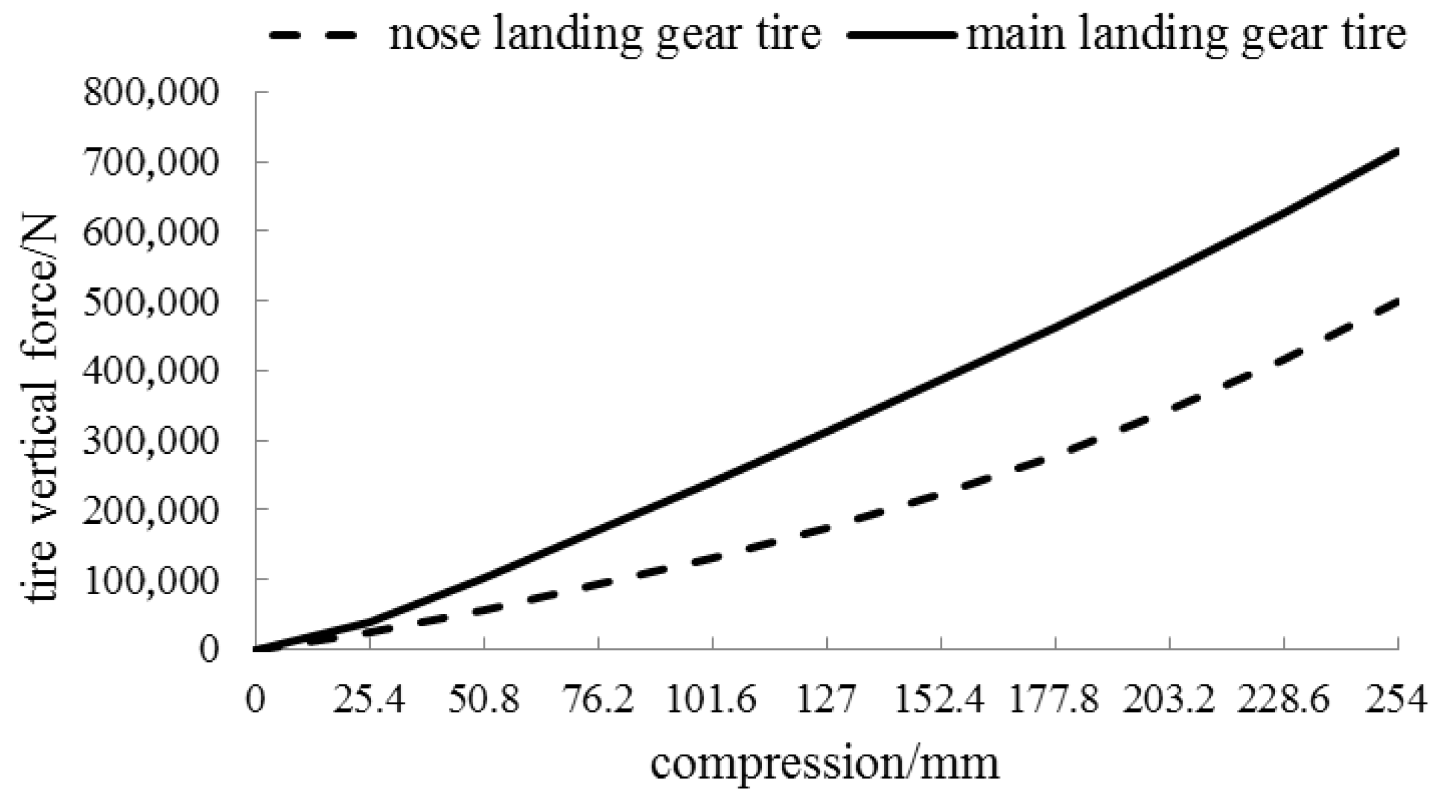
Basic data for the wheel geometry, tire pressure, mass, and moment of inertia can be obtained from the work in [20]. Based on these parameters, we selected the Fiala tire model for this study and calculated the curve of the tire’s vertical force as a function of compression, as shown in Figure 3.

2.3. Verification of Virtual Prototype Model

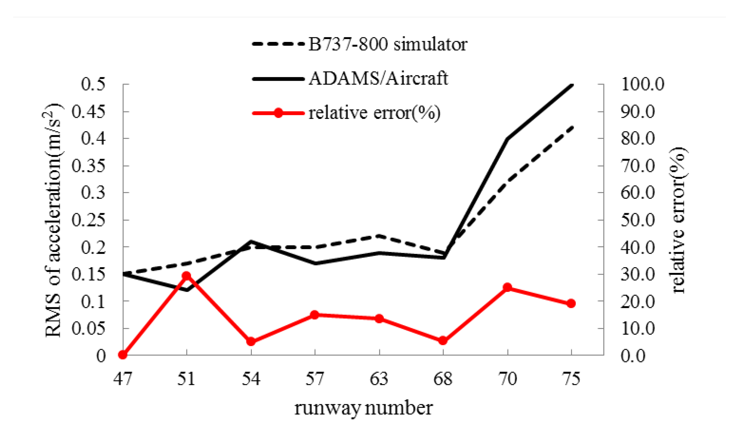
The Federal Aviation Administration (FAA) has used the B737-800 driving simulator to conduct research into airport runway roughness at the Mike Monroney Aviation Center in Oklahoma City, OK [22]. The FAA report shows the root mean square (RMS) of acceleration in an aircraft cockpit at eight actual runways. Using ADAMS/Aircraft, we controlled for the same speed and carried out simulation tests using the same runways. Figure 4 presents a comparison of the FAA simulator results and this study’s ADAMS/Aircraft-derived results. The RMS of acceleration obtained by the two methods shows similar trends. The average difference from the driving simulator was only 14% for ADAMS/Aircraft. Therefore, using ADAMS/Aircraft to implement aircraft simulations appears to be reasonable.

3. Frequency Response Function of IRI Model

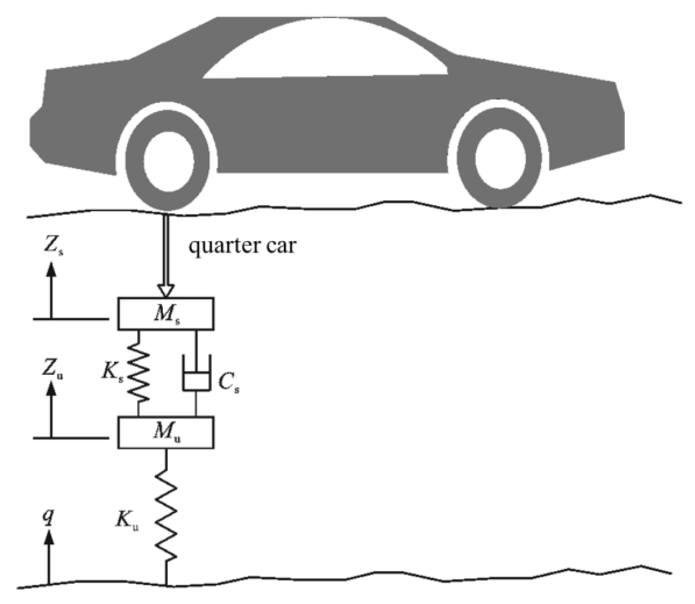
Figure 5 shows a standard 1/4 vehicle model. The unsprung mass represents the lower chassis component of the vehicle’s shock absorber and the sprung mass represents the upper component of the shock absorber. Equations (4) and (5) are the vibration balance equations for unsprung mass and sprung mass under roughness excitation, respectively.
M u Z ¨ u C s ( Z ˙ s Z ˙ u ) K s ( Z s Z u ) + K u ( Z u q ) = 0
M s Z ¨ s + C s ( Z ˙ s Z ˙ u ) + K s ( Z s Z u ) = 0
where M s is sprung mass, M u is unsprung mass, K s is the stiffness coefficient of the automobile’s suspension, C s is the damping coefficient of the automobile’s suspension, K u is the stiffness coefficient of the tire, y(x) is roughness excitation, Z s is the absolute displacement of M s , and Z u is the absolute displacement of M u .
When both sides of Equations (4) and (5) are divided by Ms at the same time, two simplified vibration balance equations are obtained, as shown in Equations (6) and (7), respectively.
U Z ¨ u C ( Z ˙ s Z ˙ u ) K ( Z s Z u ) + K ( Z u q ) = 0
Z ¨ s + C ( Z ˙ s Z ˙ u ) + K ( Z s Z u ) = 0
where C = C s + M s , K = K s + M s , U = M u / M s , and K = K u / M s .
According to the World Bank, “IRI” is defined as the cumulative value of the relative displacement of the sprung mass and unsprung mass per unit distance, which is calculated by Equation (8):
I R I = 1 L 0 L | Z s Z u | d x = 1 v t 0 t | Z ˙ s Z ˙ u | d t
where L is road length, v is driving speed, and t is driving time.
In order to find the frequency response function of the relative displacement of the sprung mass and the unsprung mass in the 1/4 vehicle model, first the IRI model equations are transformed. Equation (9) describes the relative displacement in the model.
z 1 = z s z u z 2 = z u y
Then, the displacement of the sprung mass and the unspring mass can be expressed as Equation (10).
z s = z 1 + z 2 + y z u = z 2 + y
Substituting Equation (10) into Equations (6) and (7) gives Equation (11).
z ¨ 1 + z ¨ 2 + c z ˙ 1 + k 2 z 1 = y ¨ ( u 1 ) z ¨ 2 z ¨ 1 + k 1 z 2 = ( u 1 ) y ¨
Equation (12) is used to find the frequency response function of the relative displacement.
y = e i w t z 1 = H 1 ( w ) e i w t z 2 = H 2 ( w ) e i w t
where H 1 ( w ) is the frequency response function of the relative displacement of the sprung mass and unsprung mass and H 2 ( w ) is the frequency response function of the relative displacement of the unsprung mass and roughness excitation.
Substituting Equation (12) into Equation (11), H 1 ( w ) and H 2 ( w ) are obtained, as shown, respectively, in Equations (13) and (14).
H 1 ( w ) = ( u 1 ) w 4 + k 1 ( u 1 ) w 2 w 2 k 2 w 2 + i c w k 1 ( u 1 ) w 2 + w 4
H 2 ( w ) = ( u 1 ) w 2 k 2 w 2 + i c w w 4 k 2 w 2 + i c w k 1 ( u 1 ) w 2 + w 4

4. Results and Discussion

4.1. Frequency Response Distribution of Aircraft

When the frequency of the runway surface roughness excitation is close to the natural frequency of the aircraft, significant vibration acceleration occurs. Under constant speed, the aircraft’s dynamic response is a time series of stationary random signals. Fast Fourier transform (FFT) is used to transform the time domain signal into the frequency domain to obtain the frequency characteristics of the aircraft’s vibration. Equation (15) presents the FFT.
lim T 1 T + | x ( t ) | 2 d t = lim T 1 T + F x ( 2 π f ) 2 d f = + S x ( f ) d f
In Equation (15), S x ( f ) represents the distribution of the average power (or energy) of the signal in the frequency domain, that is, the distribution of the power of the unit frequency band with frequency, which is referred to as the signal’s self-power density function. The area enclosed by the S x ( f ) and f-axis is equal to the average power of the signal x ( t ) , that is, the variance or mean square value of the amplitude distribution of x ( t ) .
Taking 37 measured runways worldwide as roughness excitation samples, we carried out a taxiing simulation test of the B737-800 virtual prototype model. Figure 6a,b show the frequency distribution of the pilot station acceleration (PSA) and the center of gravity acceleration (CGA), respectively, of the B737-800 after FFT was performed. As shown, the power spectral density of the PSA is significantly greater than that of the CGA, and the sensitive frequency of the PSA and CGA is about 0.6 Hz to 0.9 Hz.
In a 1970 study of acceleration frequency characteristics that are evident during aircraft taxiing, Morris measured the PSA and CGA by installing sensors on different aircraft [23]. The results showed that the response frequency of heavy bombers, medium bombers, transport aircraft, training aircraft, civil aviation passenger aircraft, and business aircraft is typically about 0.75 Hz to 1.2 Hz. These findings are similar to the results obtained in this study, which further shows that the use of an ADAMS/Aircraft virtual prototype to simulate an aircraft’s dynamic responses is feasible and reasonable.

4.2. Frequency Response Curves of the IRI Model and Aircraft

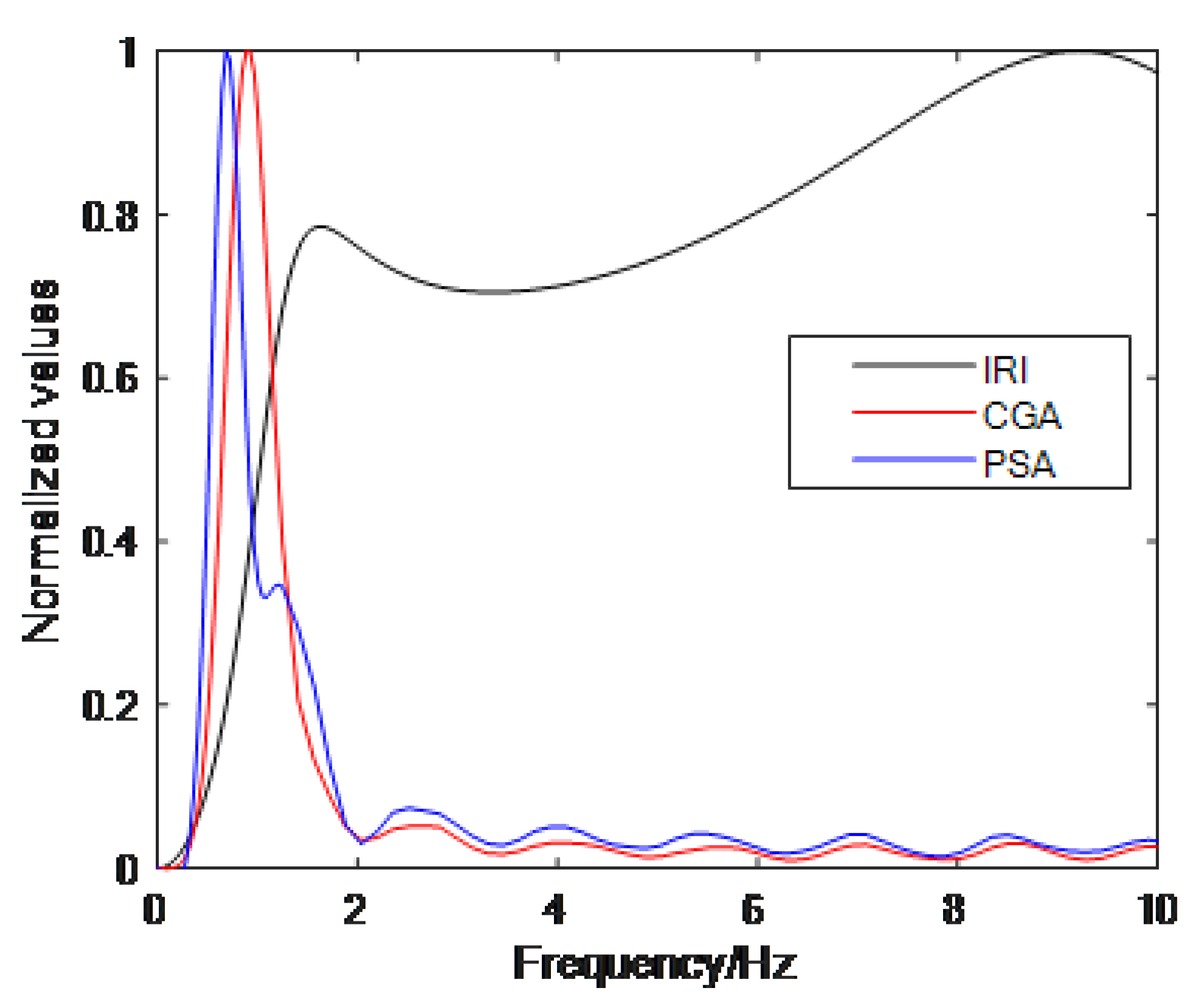
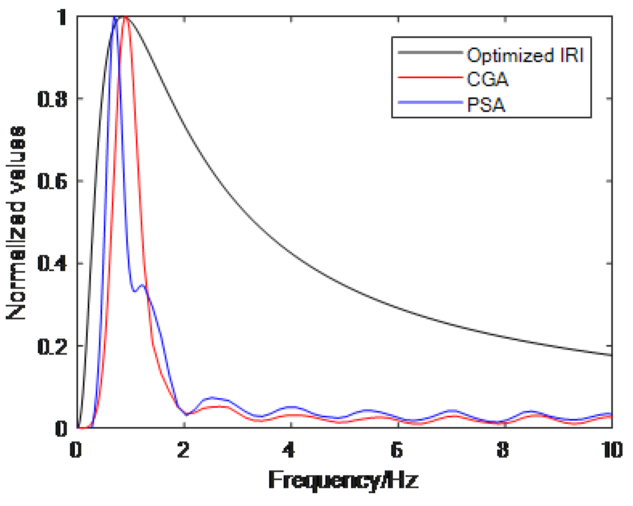
In order to eliminate any differences that could be caused by the use of different dimensions, we divided the CGA and PSA of the B737-800 model and the frequency response function of the IRI model by the maximum value of the physical quantity. Figure 7 presents the final distributions of the two models. As shown, the sensitivity of the two models to different frequency bands differs considerably. First, the IRI has the strongest frequency sensitivity at around 9 Hz, whereas the aircraft has the strongest sensitivity at 0.6 Hz to 0.9 Hz, which indicates that the aircraft’s sensitivity band is wider than that of the standard 1/4 vehicle model. Second, as the frequency increases, the two trends continue to differ. The IRI has two peaks, and the value between the two peaks is very high, but the B737 model has multiple peaks where the value at the first peak, after reaching the maximum, drops rapidly and the other peaks are at a lower level. Therefore, the substantial difference in the sensitivity bands indicates that the IRI is unable to predict the aircraft’s vibration responses effectively.

4.3. Parameter Optimization Based on Particle Swarm Optimization

Equations (13) and (14) indicate that the four parameters—c, u, k 1 , and k 2 —in the IRI model determine the sensitive frequency band. In other words, as long as a new set of [c, u, k 1 , k 2 ] is found to be consistent with the sensitive frequency band of the B737’s dynamic responses, then, theoretically, the correlation between the IRI and the aircraft’s vibration response can be improved.
To search [c, u, k 1 , k 2 ] traversally is computationally intensive and finding a set of optimal parameters is time-consuming. To address these problems, in this study, we employed an optimization algorithm to search for the best solution in the huge parameter set. Particle Swarm Optimization (PSO) is one of the most commonly used optimization algorithms [24]. This algorithm has the advantages of few parameters, strong global search capability, fast calculation speed, and fast iteration convergence. The steps taken to optimize the four parameters in this study using particle swarm optimization are as follows.
1. Initialize the attributes of the particles (number, length, position, and speed). The current position is initialized using the individual’s optimal particle best (pbest), and the current group best (gbest) is initialized using the optimal individual in the group. Each particle characterizes the corresponding whitening coefficient, and the dimensions of the particles are the same as the dimensions of the whitening coefficient.
2. Estimate the fitness function of the particles with reference to the positions of the particles. The fitness function value of each particle is measured by the mean square error (MSE), as shown in Equation (16).
fit = MSE = 1 n i = 1 n e 2 ( i )
3. Compare the fit to the p b e s t and g b e s t , respectively. If the fit is poor, then replace the p b e s t or g b e s t with the current position to obtain the current optimal whitening coefficient value.
The logic for having the particle update its own speed and position is based mainly on the individual p b e s t and the global g b e s t , as shown in Equation (17). Without exceeding the range of the given position and speed, if the value that satisfies the condition is found or the maximum number of iterations is reached, then the program is terminated.
v = v + c 1 × r 1 × ( p b e s t x ) + c 2 × r 2 × ( g b e s t x ) x = x + v
where v and x are the current velocity and position of the particle, respectively; v and x are the updated velocity and position of the particle, respectively; r 1 and r 2 are random numbers between 0 and 1; and c 1 , c 2 are learning factors.
The number of particles used in this study is four, which represents [c, u, k 1 , k 2 ]. The fitness function is the difference between the two curves in Figure 8 after optimizing the IRI model. The constraint is the premise of ensuring that the most sensitive frequencies are consistent. The trends for the other frequency bands are as similar as possible. Finally, the parameters determined by PSO after optimization of the IRI model are u = 0.0125 , c = 6.235 , k 1 = 30.64 , and k 2 = 10.85 . Figure 8 shows the difference in sensitivity to the different frequency bands between the optimized model and the B737 model. Obviously, the optimized IRI model is closer to the frequency-sensitive characteristics of the CGA of the B737 than the original IRI model.

4.4. Case Study

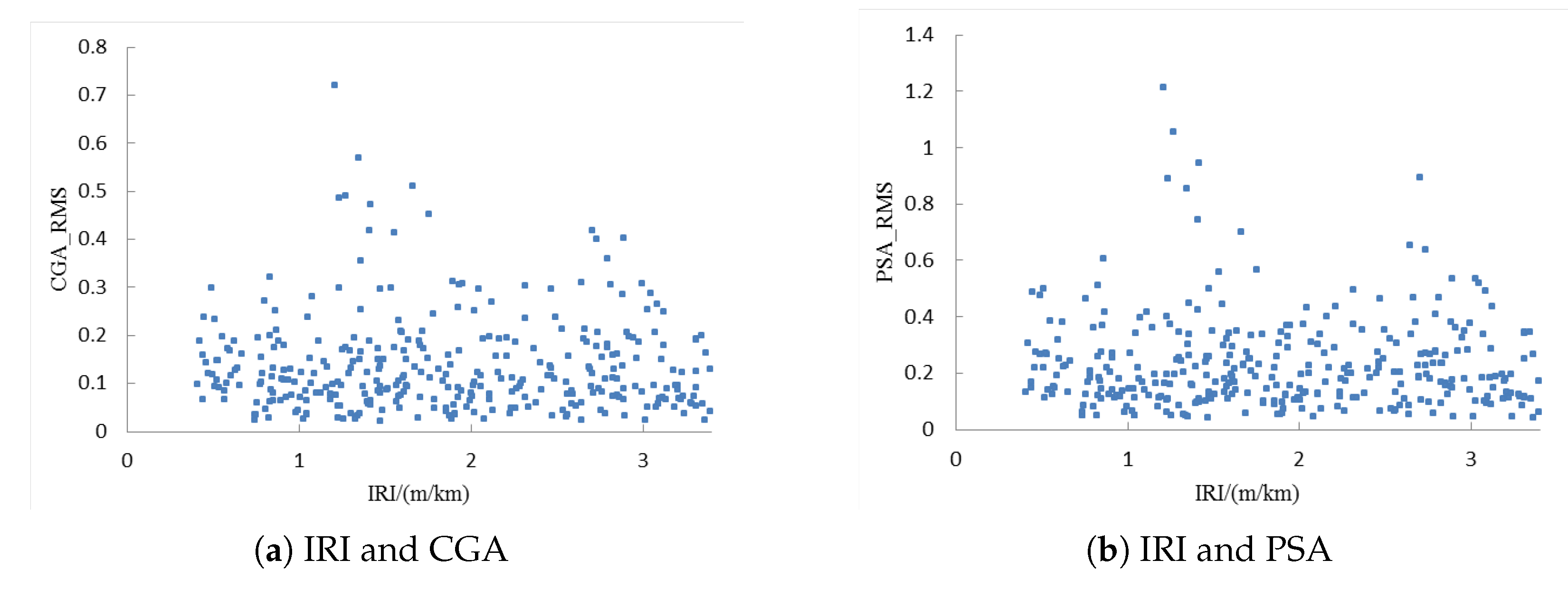
In this study, we collected runway data for Shanghai Pudong Airport Runway No. 4, Hangzhou Xiaoshan Airport Runway No. 1, Dongying Shengli Airport Runway, Ningbo Lishe Airport Runway, and Nanjing Lukou Airport Runway No. 1. We collected the aircraft dynamic response data through B737-800 virtual prototype. At a statistical interval of 50 m, we collected 342 effective samples. As shown in Figure 9, the abscissa is the root mean square (RMS) of the CGA and PSA. Generally, the RMS of the CGA is distributed between 0 m/ s 2 and 0.8 m/ s 2 , whereas the RMS of the CGA is between 0 m/ s 2 and 1.4 m/ s 2 . These results indicate that the roughness distribution of the five runways is wide and the differences are obvious. Therefore, this research into the IRI’s relevance is representative.
Figure 9 and Figure 10 show the correlation between the original IRI values and the optimized IRI values with aircraft responses, respectively. The distribution of the IRI values and RMS of the CGA and PSA present random state, which is of little significance through linear fitting. This outcome indicates that characterizing airport runway roughness based on the index vibration response of a 1/4 vehicle is unreasonable. The correlation between the optimized IRI and RMS of the CGA has strengthened significantly, and the linear fitting coefficient is up to 0.63. Similarly, the correlation between the optimized IRI and PSA also increased significantly to 0.56.

5. Conclusions

In this study, we modified the IRI model parameters in order to adapt the IRI so that it can be used to evaluate airway runway roughness, not just roadway roughness. Using ADAMS/Aircraft software, we established and validated a detailed B737-800 virtual prototype model. We analyzed and compared the frequency response functions of the IRI model and the B737-800 model. Using PSO, we optimized the IRI model parameters. The following conclusions can be drawn.
  • The B737-800 virtual prototype model developed and validated in this study is reliable and can represent aircraft dynamic responses to rough runways.
  • The frequency response curves of the IRI model and aircraft model differ greatly, which indicates that the IRI cannot effectively represent the vibration responses of aircraft to runway roughness.
  • PSO accelerates the efficiency of parameter optimization. The optimized IRI model approximates the vibration response characteristics of the aircraft better than the original IRI model (without optimized parameters).
  • The case study results show that the correlation coefficient between the optimized IRI model and the aircraft vibration response is as high as 0.56. Compared with the original IRI model, the optimized IRI model shows a qualitative leap in terms of correlation coefficients.

Author Contributions

Conceptualization, S.L. and Y.T.; methodology, S.L. and Y.T.; validation, S.L. and Y.T.; investigation, S.L. and Y.T.; resources, S.L. and Y.T.; data curation, S.L. and Y.T.; writing—original draft preparation, S.L. and Y.T.; writing—review and editing, S.L., Y.T., L.L., and P.X.; visualization, S.L. and Y.T.; supervision, S.L. and Y.T.; project administration, S.L. and Y.T.; funding acquisition, S.L. and Y.T. All authors have read and agreed to the published version of the manuscript.

Funding

This study was supported by China Postdoctoral Science Foundation funded project (No.2020M681392), and the National Natural Science Foundation of China (Grant No. U1833123 and No.U1933113). The authors appreciate the help of Zhekai Zhang, Junjun Chen, Penghui Li, et al.

Institutional Review Board Statement

Not applicable.

Informed Consent Statement

Not applicable.

Data Availability Statement

[1]. The [Airframe aerodynamics, Landing gear buffer system, wheels] data presented in this study are available on request from the corresponding author. The data are not publicly available due to [institution policy] [2]. The [runway profile data for Shanghai Pudong Airport Runway No. 4, Hangzhou Xiaoshan Airport Runway No. 1, Dongying Shengli Airport Runway, Ningbo Lishe Airport Runway, and Nanjing Lukou Airport Runway No. 1. ] data presented in this study are available on request from the corresponding author. The data are not publicly available due to [airports internal policy]. [3]. Publicly available datasets were analyzed in this study. [B737-800 simulator] data can be found here: [https://www.airporttech.tc.faa.gov/Products/Airport-Pavement-Papers-Publications/Airport-Pavement-Detail/ArtMID/3684/ArticleID/159/Boeing-737-800-Final-Surface-Roughness-Study-Data-Collection (accessed on 13 February 2021)]. [4]. These prior studies (and datasets) are cited at relevant places within the text as references [F.A.A., Surface Roughness Study Final Data Report Boeing 737–800. Washington, DC: Federal Aviation Administration, 2015].

Conflicts of Interest

The authors declare no conflict of interest.

References

  1. Gerardi, A.G. Dynamic Response of Aircraft to Pavement Unevenness; Transportation Research Board Special Report; TRB: Washington, DC, USA, 1978. [Google Scholar]
  2. Gervais, E.L. Runway roughness measurement, quantification and application: The Boeing approach. In Aircraft/Pavement Interaction: An Integrated System; ASCE: Reston, VA, USA, 1991; pp. 121–131. [Google Scholar]
  3. Civil Aviation Administration of China. MH/T 5024-2009, Technical Specifications of Aerodrome Pavement Evaluation and Management. 2009. Available online: https://www.docin.com/p-119165177.html (accessed on 13 February 2021).
  4. Transport Canada, Measurement and Evaluation of Runway Roughness. Civil Aviation, Standards. Advisory Circular AC 302-023, 16 September 2015. Available online: https://tc.canada.ca/sites/default/files/migrated/ac_302_023_issue_02.pdf (accessed on 13 February 2021).
  5. Hayhoe, G.F. Airport pavement rideability rating for maintenance evaluation. In Proceedings of the 2016 Airports Conference, Hershey, PA, USA, 21–23 March 2016; Volume 22. [Google Scholar]
  6. Sayers, M.W. The International Road Roughness Experiment: Establishing Correlation and a Calibration Standard for Measurements; Technical Report; University of Michigan, Ann Arbor, Transportation Research Institute: Ann Arbor, MI, USA, 1986. [Google Scholar]
  7. Emery, S.; Hefer, A.; Horak, E. Roughness of runways and significance of appropriate specifications and measurement. In Proceedings of the 11th Conference on Asphalt Pavements for Southern Africa, Sun City, South Africa, 16–19 August 2015. [Google Scholar]
  8. Loprencipe, G.; Zoccali, P. Comparison of methods for evaluating airport pavement roughness. Int. J. Pavement Eng. 2019, 20, 782–791. [Google Scholar] [CrossRef]
  9. Chen, Y.; Chou, C. Effects of airport pavement-profile wavelength on aircraft vertical responses. Transp. Res. Rec. 2004, 1889, 83–93. [Google Scholar] [CrossRef]
  10. Ling, J.M.; Liu, S.F.; Yuan, J.; Yang, W.c. Applicability of IRI based evaluation of airport pavement roughness. J. Traffic Transp. Eng. 2017, 17, 20–27. [Google Scholar]
  11. Cardoso, S.H. Aircraft-based pavement surface roughness assessment. Transp. Res. Rec. 2007, 2007, 104–110. [Google Scholar] [CrossRef]
  12. Chen, Y.; Chou, C. Assessment of Aircraft’s Vertical Responses to Develop the Roughness Evaluation Index for Airport Pavement by; Citeseer: Princeton, NJ, USA, 2004. [Google Scholar]
  13. Woods, J.E. A Study of Airport Pavement-Aircraft Interaction Using Wavelet Analysis; The University of Texas at San Antonio: San Antonio, TX, USA, 2008. [Google Scholar]
  14. Major, W.; Matthew, J.; Hubbard, S.; Bullock, D. Evaluation of opportunities for connected aircraft data to identify pavement roughness at airports. Coll. Aviat. Rev. Int. 2018, 36. [Google Scholar] [CrossRef] [Green Version]
  15. Cheng, G.; Guo, W. Airport pavement roughness evaluation based on three-degree-of-freedom aircraft model. J. Nanjing Univ. Aeronaut. Astronaut. 2016, 48, 606–614. [Google Scholar]
  16. Kanazawa, H.; Su, K.; Noguchi, T.; Hachiya, Y.; Nakano, M. Evaluation of airport runway pavement based on pilots’ subjective judgement. Int. J. Pavement Eng. 2010, 11, 189–195. [Google Scholar] [CrossRef]
  17. Dong, Q.; Hachiya, Y.; Endo, K.; Himeno, K.; Kawamura, A.; Matsui, K. Airport pavement roughness evaluation based on aircraft response. In Health Monitoring and Smart Nondestructive Evaluation of Structural and Biological Systems III; International Society for Optics and Photonics: Bellingham, WA, USA, 2004; Volume 5394, pp. 118–126. [Google Scholar]
  18. Endo, K.; Himeno, K.; Kawamura, A.; Hachiya, Y.; Matsui, K. Evaluation of longitudinal runway profile and ride quality using wavelet analysis and brain waves. In Proceedings of the TRB 82nd Annual Meeting, Washington, DC, USA, 12–16 January 2003. [Google Scholar]
  19. Liu, S.; Ling, J.; Yuan, J.; Li, P.; Chen, J. Landing gear cumulative stroke-based runway roughness evaluation. In Proceedings of the 97th Annual Meeting of Transportation Research Board, Washington, DC, USA, 7–11 January 2018. [Google Scholar]
  20. Boeing Commercial Airplanes. 737 Airplane Characteristics for Airport Planning; Technical Report D6-58325-6; Boeing Commercial Airplanes: Seattle, WA, USA, 2020. [Google Scholar]
  21. Koşar, K.; Durmaz, S.; Jafarov, E.M. Longitudinal dynamics analysis of Boeing 747-400. In Proceedings of the 9th WSEAS International Conference on Automatic Control, Modelling and Simulation, Istanbul, Turkey, 27–29 May 2007; pp. 82–87. [Google Scholar]
  22. F.A.A. Surface Roughness Study Final Data Report Boeing 737-800; Federal Aviation Administration: Washington, DC, USA, 2015. [Google Scholar]
  23. Morris, G.J. Response of Several Turbojet Airplanes to Runway Roughness; National Aeronautics and Space Administration: Washington, DC, USA, 1970; Volume 5740. [Google Scholar]
  24. Cai, X.; Gao, L.; Li, F. Sequential approximation optimization assisted particle swarm optimization for expensive problems. Appl. Soft Comput. 2019, 83, 105659. [Google Scholar] [CrossRef]
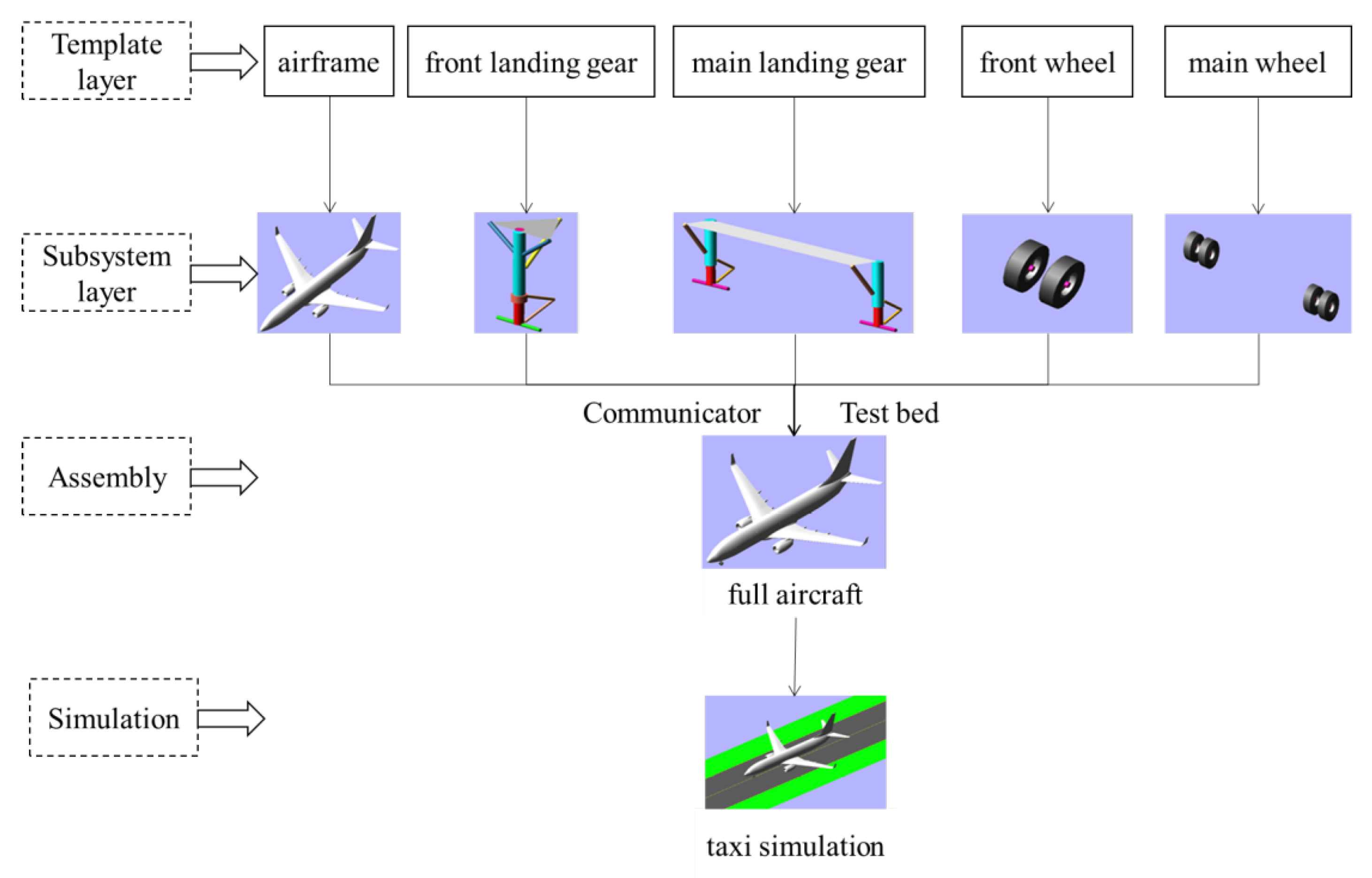
Figure 1. Aircraft taxi simulation in ADAMS/Aircraft [19].
Sustainability 13 02184 g001
Figure 2. Air spring force versus compression stroke curve.
Sustainability 13 02184 g002
Figure 3. Tire vertical force versus compression curve.
Sustainability 13 02184 g003
Figure 4. Comparison of results obtained from two different simulation methods.
Sustainability 13 02184 g004
Figure 5. Quarter vehicle model.
Sustainability 13 02184 g005
Figure 6. Sensitive frequency of B737-800 in terms of power spectral density (PSD): (a) pilot station acceleration (PSA) and (b) center of gravity acceleration (CGA).
Sustainability 13 02184 g006
Figure 7. Sensitivity of International Roughness Index (IRI) model and B737 model’s center of gravity acceleration (CGA) to different frequency bands.
Sustainability 13 02184 g007
Figure 8. Sensitivity of optimized model and B737 model to frequency bands.
Sustainability 13 02184 g008
Figure 9. Correlation between original IRI values and the root mean square (RMS) of the aircraft’s CGA and PSA data.
Sustainability 13 02184 g009
Figure 10. Correlation between optimized IRI and RMS of of the aircraft’s CGA and PSA data.
Sustainability 13 02184 g010
Table 1. Mass, moment of inertia, and location of center of gravity for B737-800 [20].
MassEstimated Moment of InertiaCenter of Gravity
MTW/kg78,472 Iy / kg · m 2 3,394,95313.60 m to nose
landing gear
MTOW/kg78,245 Ix / kg · m 2 1,866,711
MLW/kg65,317 Iz / kg · m 2 5,097,558
Note: MTW is Maximum TaxiWeight; MTOW is Maximum Takeoff. Weight; MLW is Maximum Land Weight.
Table 2. Wing attribute parameters of aircraft model.
Aircraft S R E F / f e e t 2 SPAN/mMAC/mAspect Ratio
B737-800134135.793.799.45
Publisher’s Note: MDPI stays neutral with regard to jurisdictional claims in published maps and institutional affiliations.