Article

Cross-Validation of the MEDEAS Energy-Economy-Environment Model with the Integrated MARKAL-EFOM System (TIMES) and the Long-Range Energy Alternatives Planning System (LEAP)

1
Consorzio Interuniversitario Nazionale per la Scienza e la Tecnologia dei Materiali (INSTM), c/o Dipartimento di Chimica, Università degli Studi di Firenze, Via della Lastruccia 3, 50019 Sesto Fiorentino, Firenze, Italy
2
Global Sustainability Institute, Anglia Ruskin University, East Road, Cambridge CB1-1PT, UK
3
Black Sea Energy Research Centre, 7 Victor Grigorovich Str., 1606 Sofia, Bulgaria
4
Austrian Energy Agency (AEA), Mariahilfer Straße 136, 1150 Wien, Austria
5
Centre de Recerca Ecològica i Aplicacions Forestals (CREAF), Campus de Bellaterra UAB, Edifici C, 08193 Barcelona, Spain
6
Departament d’Enginyeria Mecànica, Universitat Rovira i Virgili (URV), Campus Sescelades, Avinguda dels Països Catalans, 26, 43007 Tarragona, Spain
*
Author to whom correspondence should be addressed.
Sustainability 2021, 13(4), 1967; https://doi.org/10.3390/su13041967
Submission received: 12 January 2021 / Revised: 4 February 2021 / Accepted: 6 February 2021 / Published: 11 February 2021
(This article belongs to the Section Energy Sustainability)

Abstract

:
In the present study, we compare energy transition scenarios from a new set of integrated assessment models, the suite of MEDEAS models, based on a systems dynamic modeling approach, with scenarios from two already well know structurally and conceptually different integrated assessment models, the Integrated MARKAL-EFOM System (TIMES) and the Long-Range Energy Alternatives Planning system (LEAP). The investigation was carried out to cross-compare and benchmark the response of MEDEAS models with TIMES and LEAP in depicting the energy transition in two different countries, Austria and Bulgaria. The preliminary results show a good agreement across all the models in representing scenarios projecting historical trends, while a major discrepancy is detectable when the rate of implementation of renewable energy is forced to increase to achieve energy system decarbonization. The discrepancy is mainly traceable to the differences in the models’ conception and structures rather than in a real mismatch in representing the same scenarios. The present study is put forward as a guideline for validating new modeling approaches that link energy policy decision tools to the global biophysical and socioeconomic constraints.

1. Introduction

The dynamics of complex systems, like socio-economic systems, energy systems, and environmental systems, are all interconnected by a dense network of feedbacks. Through to the development of integrated assessment models (IAMs), which link socioeconomic, energy, and environmental models, it is possible to simulate simultaneously human and environmental systems, implementing dynamics related to society and economy with dynamics in the biosphere and atmosphere into a single modeling framework [1,2]. Since the precursor World3 model [3], several IAMs have been created: However, especially those with greater influence over policy, share a core set of assumptions whose validity is still disputed in the scientific community, underpinning the development of new models [4].
The MEDEAS suite of models [5] is a set of mathematical models that aims to improve the state-of-the-art of IAMs: System dynamics modeling approach makes MEDEAS able to overcome the traditional IAMs sequential structure that allows only for a restricted number of feedbacks among the represented subsystems. Indeed, the highly aggregated nature of the dynamics simulated with IAMs usually translates in an oversimplification of the dynamics related to the economic dimension, e.g., by using aggregated production functions and using prices as indicators of scarcity [6]. Additional limitations of IAMs are the absence of physical limits to the installation of renewable energy sources (RES), and, most relevant, IAMs often omit climate change assessment and impacts [7,8,9]. The approach used in MEDEAS proposes an innovative modeling framework (Figure 1), integrating global biophysical and socioeconomic constraints to support the design of policy. Despite their short existence, the MEDEAS models have already been used to study different aspects of the energy–economy–environment interrelations in several publications; for more detail, the reader is referred to references [10,11,12,13] and the project website [14].
Considering new limits for RES and the impacts of climate change, MEDEAS configures as a more advanced IAM, providing new perspectives on the actions required for the transition, identifying new topics that need attention and further study, for instance, scarcity of the rare earth metals needed to develop energy storage [15,16]. MEDEAS also configures as powerful tools to give insight on ‘decoupling’ strategies [17]: In MEDEAS, economic demand is estimated from exogenous pathways of expected per capita gross domestic product and population evolution [5,13].
MEDEAS models, initially developed in Vensim®, have an open-source version in the Python programming language, the pymedeas models, which provide three geographical levels: World, EU 28, and Austria (pymedeas_w, pymedeas_eu, and pymedeas_at) [10]. The structure of MEDEAS set of models is nested, meaning that some outputs from the simulations of the world model become inputs to the European model, whose output are in turn used as inputs to the country models.
In this work, we benchmark the outputs of the MEDEAS country models (Austria and Bulgaria) against The Integrated MARKAL-EFOM System (TIMES) model of the Austrian energy system [18,19] for Austria (TIMES_at) and the Long-Range Energy Alternatives Planning system (LEAP) for Bulgaria [20] (LEAP_bg).
TIMES and LEAP are two model generators. TIMES is an energy system model generator that strictly uses linear optimization to produce a least-cost energy system, optimized according to several constraints. The main outputs from TIMES are energy system configurations, which meet the end-use energy service demands, at least cost, while also adhering to various constraints set by the user. TIMES supports the simulation of dynamics related to all technologies available for thermal, renewable, storage/conversion, and transport [21].
LEAP is an integrated, scenario-based, linear modeling tool that accounts for both the energy sector and non-energy sector greenhouse gas (GHG) emission sources and sinks [20]. The LEAP modeling procedure asks the user to specify key non-energy assumptions (demographic, macroeconomic, etc.), energy demand, energy losses, own needs, exogenous and endogenous production capacities, import/export so that LEAP calculates the necessary energy production, additional capacities needed, primary energy requirements, emissions, and costs.
Unlike TIMES and LEAP linear modeling, and as mentioned before, the MEDEAS set of models were developed using the system dynamics approach, which facilitates the integration of interdisciplinary subsystems and dynamics, as well as interactions between them, therefore allowing to capture of non-linearities in the energy system. The general differences (qualitative comparison) between the MEDEAS, TIMES, and LEAP approaches (types of models [21], purposes [22]) are reported at the Medeas project website [23].
In the present study, TIMES_at and LEAP_bg are no longer model generators, but the actual specific models adapted for the two countries from the respective national energy agencies: The Austrian Energy Agency (AEA) for TIMES_at and the Black Sea Energy Research Centre (BSERC) for Bulgaria. TIMES_at and LEAP_bg have been used and continuously developed by the energy agencies for years, giving a reliable representation of all the sectors of the respective national energy systems. For this reason, TIMES_at and LEAP_bg are used as benchmarks to test the results of the respective MEDEAS models for Austria and Bulgaria.
The comparison aims to verify if the MEDEAS country models’ projections are in agreement, within acceptable ranges, with those produced by LEAP_bg and TIMES_at models.
While the World and EU MEDEAS models have already been presented and discussed in the literature [5,10,13,16,24,25], until the current work, the MEDEAS country models for Austria and Bulgaria had not been the subject of any publication. Hence, the current work aims to present the adaptation of the MEDEAS models to a smaller regional scale as well as to test their validity by benchmarking their results against the well-known TIMES and LEAP models.

2. Materials and Methods

In this section, we describe the methodologies used for the cross-validation. Three main aspects are presented: identification of appropriate scenarios to be compared across the models; identification of the variables to be compared within each scenario across the models; method to compare the selected variables.
The models’ outputs to be compared are those generated simulating two long term scenarios: The business as usual (BAU) and optimal level transition (OLT) scenarios, each one adapted to Austria and Bulgaria respective energy–economy–environment structures.
The BAU scenario allows the variables of the model to evolve in the future following historical trends and current and currently planned policies, while, OLT represents a scenario based mainly on improvements in energy efficiency and implementing renewable energy, to accomplish national decarbonization according to the goals of the Paris Agreement [26]. In this regard, the constraint of the Paris agreement has been evaluated in terms of national carbon budgets between 2012 and 2050, calculated for Austria (1.85 GtCO2 eq) and Bulgaria (1.45 GtCO2 eq) with the methodology developed by Perissi et al. [27] and summarized in Appendix A. The scenario based on decarbonization hypothesis is the starting point to represent a reference estimation for the end goal of a decarbonizing transition that is compatible with the achievement of the Paris goal. A discussion on the possible achievement or failure of this national budget goal is outside of the aim of the present paper (focused on comparing modeling tools) and will be addressed in future works.
To compare the models’ behaviors, several methodologies can be used, including the root means squared differences (RMSDs), percent variance, and maximum likelihood [28]. RMSDs and maximum likelihood are similar methodologies, however, the RMSDs approach is more intuitive [29,30], especially when independent variables are not random, as in the present case, in which the investigated variables are functions of time series. Moreover, RMSDs is easy to compute and applies to many types of models and types of data, including projections: the lower the RMSD, the smaller the discrepancy between the models under comparison. The RMSDs have the same units of the variables involved in their computing, which is a useful feature to rapidly evaluate the differences of the trajectories generated by MEDEAS with the ones generated by the benchmarking models.
The RMSDs were calculated to compare the outputs of the MEDEAS country models for Austria and Bulgaria with those of the respective Austrian and Bulgarian national models, TIMES_at and LEAP_bg. However, in the present case, the cross-validations for modeling tools assume a slightly different meaning. For each of the pairs of outputs (for instance, one output series from MEDEAS_at and one output series from TIMES_at), we calculated the RMSD in absolute values (listed in Table 1 and Table 2) and with normalized values (listed in Table 3 and Table 4). RMSDs in absolute values have the same unit as the variable they refer to, thus the principle that the smaller is RMSD, the better is the accordance between the outputs, is not valid because the magnitude of RMSD depends on the unit used to measure the variable. However, RMSDs in absolute values are useful to assess the deviation of the same variable in the two different scenarios, BAU and OLT.
Normalized RMSDs are instead suitable to compare the differences among all considered variables within the models of the same country (considering the principle of the smaller RMSDs). Though there are no consistent methods of normalization in the literature, common choices are the mean [31] or the range (defined as the maximum value minus the minimum value) of the reference data. In the present study, we opted for the mean, to avoid indetermination in case of the difference between the maximum and the minimum of the series was small.
As reference series, we take the means of MEDEAS variables so that it is also possible to assess which of the two benchmarking models (TIMES_at and to LEAP_bg) has more or fewer similarities to the respective MEDEAS country.
The calculation of RMSDs has been automated using a MATLAB® script. The algorithm calculated RMSD for each pair of data as follows:
  • Standard (or absolute) RMSDs:
R M S D j   =   t   =   1995 2050 M E t , j   T L t ,   j 2 2050 2010 .
  • Normalized RMSDs:
R M S D j = 1 t T M E t , j / T t + 1 t T M E t , j T L t , j 2 T t + 1 ,
where M E t , j and T L t , j represent the data of any output variables j at time t, (for instance, considering M E t , j the data of MEDEAS_model and T L t , j the data of TIMES or LEAP, within the same scenario).
Note that the code also adjusts the units of measurement and provides graphs depicting the RMSDs as a function of the respective pairs of variables. It also provides RMSDs outputs every five years in the interval between 2025 and 2050 starting from 2010, to assess how the variances evolve across the time series.
The absolute and normalized RMSDs have been calculated for Austrian and Bulgarian country models within the two different scenarios under study: BAU and OLT.
For Bulgaria, the algorithm is slightly different in comparison to the one used for Austria as the input files of the two MEDEAS models are not the same. This reflects peculiarities in the energy system of the two countries. However, conceptually, the code executes the same calculations. The dimension adjustment on output units has been taken into account, they are reported and labeled in the MATLAB codes in Appendix B.
In addition, TIMES_at and LEAP_bg are based on an integrated approach of modeling methodologies and they are energy-system models thus, mainly the energy market variables (Table 1 and Table 2) of the four models will allow for the cross-comparison within a set of designed transition scenarios. On the other hand, MEDEAS models take into account not only energy markets but also energy and resource availability. The main feedbacks to the economy module from the rest of the model are delivered by climate change impacts and energy supply availability. Thus, to perform the comparison, only energy-related feedbacks are activated, to optimize the MEDEAS assumptions to fit the TIMES and LEAP assumptions (e.g., renewable capacities).

3. Results

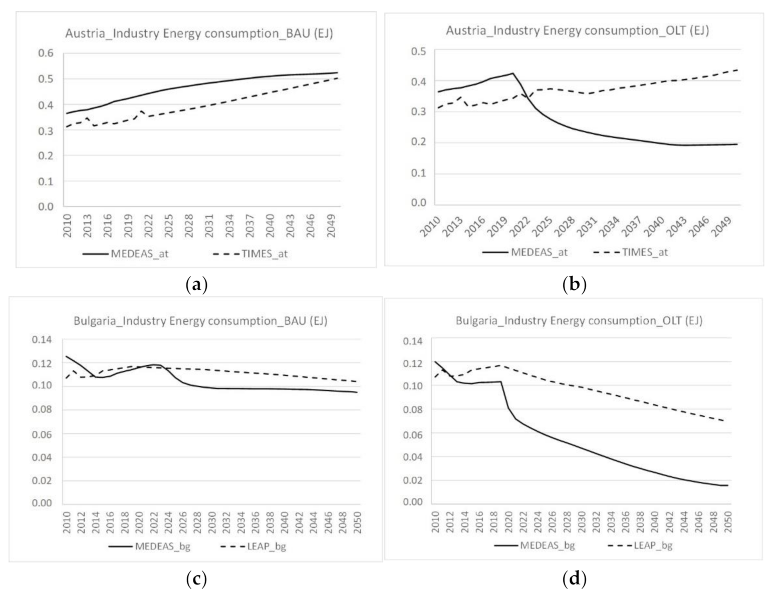
The images below show the energy consumption for the industry sector in Austria and Bulgaria for BAU and OLT scenarios.
The previous Figure 2 is an example of the kinds of comparisons that are made between the three models. The decrease of industry energy consumption in both Austria and Bulgaria OLT scenarios is due to a mix of increased technical efficiency and scenario assumptions. Indeed, the characteristics of the OLT scenario, which is focused on Greenhouse Gases (GHG) emissions reduction (carbon budget limitations), leads to reduced realizable economic growth, much lower economic demand, lower energy consumption in all sectors, including industry (details on scenarios assumptions are available at Project Medeas website [32]).
All the RMSDs are reported, in correspondence with each pair of considered variables, in Table 3 (Standard BAU) and Table 4 (Standard OLT), Table 5 (Normalized BAU), and Table 6 (Normalized OLT) for Austria; in Table 7 (Standard BAU) and Table 8 (Standard OLT), Table 9 (Normalized BAU), and Table 10 (Normalized OLT) for Bulgaria.
The RMSDs give information on the level of agreement between the curves, allowing also for qualitative comparisons of the time-series across all the investigated models.
As previously introduced, to assess the overall similarity between the benchmarking models (LEAP_Bg and TIMES_at) and MEDEAS country models across all the variables and the scenarios, we calculated the distribution of the normalized RMSDs with respect to the mean of the MEDEAS series of data.
The normalized RMSDs have been calculated every ten years since 2010 to 2050 (2010–2030, 2010–2040, 2010–2050) to analyze the variances among the variables to evaluate the response of models over time. We included the historical data (2010–2020) in the RMSDs calculation to account also for the difference in the historical sources between the benchmarking models and MEDEAS countries.
With the normalized RMSDs distribution we highlight how many and which variables series shows lower normalized RMSDs, representing a good agreement between MEDEAS and national models, or instead how many show higher RMSDs, representing the low resemblance between MEDEAS and both TIMES and LEAP outputs, investigating, at the same time, the models’ temporal variances’ response.

3.1. Results for Austria

The RMSDs distribution in absolute values for Austria is reported in Table 3 and Table 4. Variables energy units are in Exajoule (EJ) if not differently specified (i.e., for “share” variables).
Comparing the series for Austria in absolute values, most of the variables that TIMES and MEDEAS have in common show similar RMSDs for the BAU and the OLT scenarios.
The most important differences are visible for variables 2 (transport), 5, 6, 7 (fossil extraction), 10 (biomass requirement), 11 (heat), 23 (share of electricity in transport). These results suggest that these variables are probably the most affected by the initial condition and evolution of the scenarios from BAU to OLT.
A key difference in RMSD values is seen in variables that are characterized by an exponential growth in MEDEAS compared to stable growth (or no growth) in TIMES. These behaviors in BAU scenarios have been observed for variable 11 (heat-real FE consumption by fuel in MEDEAS_at and district heat in TIMES_at), variable 2 (real final energy by sector and fuel AUT [transport] in MEDEAS_at and Export-EEVbySector-en-Transport for TIMES_at), variable 5 (PES fossil fuel extraction [scenarios, gases] in MEDEAS_at and Export-BIV-en-Fossil fuels gaseous in TIMES_at) and variable 6 (PES fossil fuel extraction [scenarios, solids] in MEDEAS_at and Export-BIV-en-Fossil fuels solids in TIMES_at). This is mainly due to the unrestricted availability of resources in MEDEAS models, and to the fact that the projections in TIMES_at are instead almost stable for the whole period.
For the same variables (2, 5, and 6), RMSDs decrease in the respective OLT scenarios, where both MEDEAS_at and TIMES_at show declining trends.
Variables related to liquids show the opposite trends. Variable number 7 (PES fossil fuel extraction [scenarios, liquids] in MEDEAS_at and Export-BIV-en-Fossil fuels liquids in TIMES_at) shows higher RMSD for OLT scenarios, mainly due to the deep phasing out of liquids in TIMES_at projections between 2030 and 2050. Variables 17–23, which describe the projections of RES capacity installation and the projections of GHG emissions by sectors, show a very good agreement in being represented by TIMES_at and MEDEAS_at models for both BAU and OLT scenarios.
Regarding the achievement of the national budget within the OLT scenario, TIMES_at show simulated budget quite close to the national objective, around 2.5 GtCO2 eq. MEDEAS_at results in a cumulative emissions simulation double than TIMES_at. The order of magnitude is the same, the major deviation of MEDEAS_at is again due to setting unrestricted availability of resources in MEDEAS models.
This suggests that, for Austria, the increase in renewable implementation rates is the main action that would lead to national decarbonization in the frame of the Paris goal. Further studies will point out a more exhaustive decarbonization strategy.
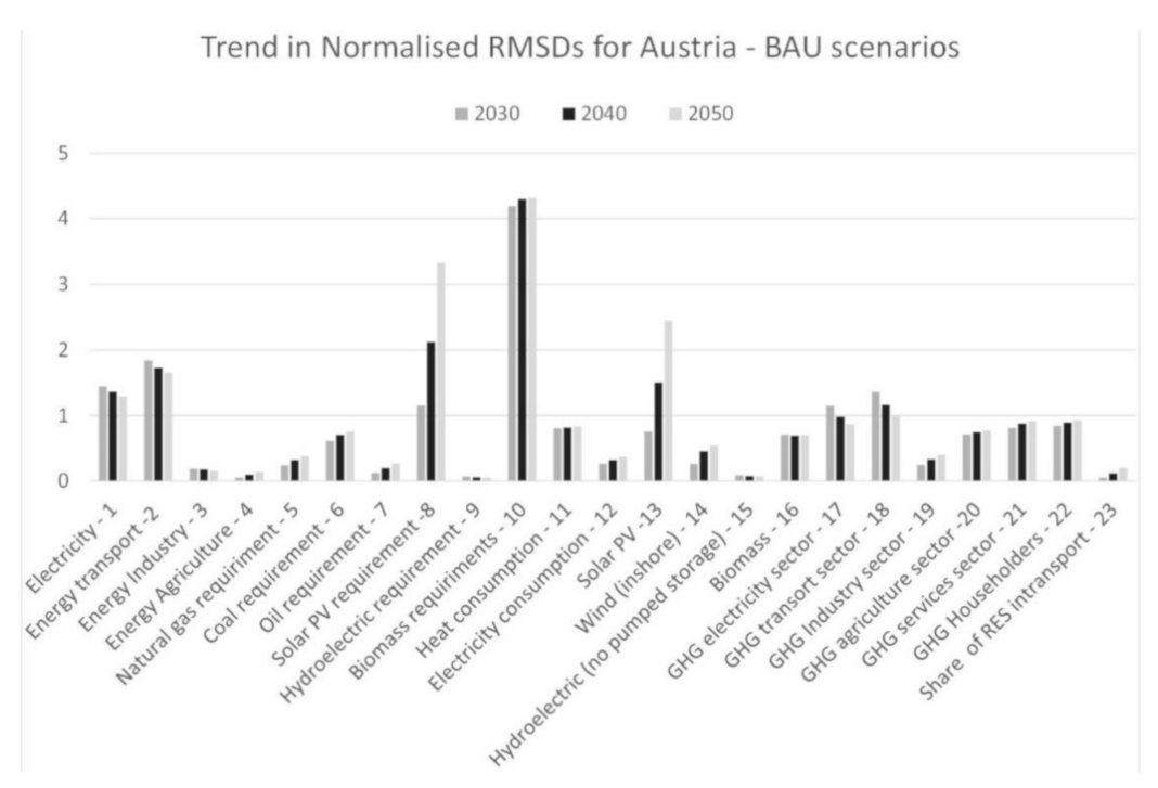
Comparing the series in normalized values for the Austrian BAU scenario (Table 5), it is then possible to explore the difference between variables across the whole data series behaviors (Figure 3).
Decreases in RMSDs over time can be observed, in variables 1 (electricity), 2 (energy in transport), 9 (hydroelectric requirement), 15 (hydroelectric pumped storage), 17 (electricity sector), and 18 (transport). Thus, variable 1 and 9 results are more affected by the difference in the initial conditions but the discrepancy tends to diminish gradually as both TIMES and MEDEAS approach the 2050 decarbonization goal. This is also evident in variables 17 and 18, which describe the related GHG emissions.
The deviation for PV variables 8 and 13 increase three times in 2050, since TIMES_at considers a nearly linear increase on PV development while in MEDEAS_at, the variable (all variables related to renewables) grow exponentially according to a set growth rate.
The change in RMSDs with time for the other variables are minor, reflecting a good agreement with the simulations between the two models.
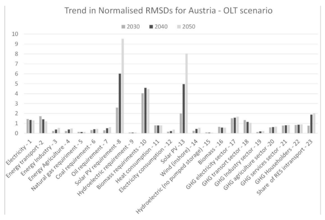
In the OLT scenario (Table 6, Figure 4), the variances for the PV variables 8 and 13 increase are even higher, highlighting again that TIMES_at considers an almost linear increase on PV development while in MEDEAS_at, the variable (all variables related to renewables) grows exponentially.
The change in RMSDs with time for the other variables is minor, reflecting a good agreement with the simulations between the two models.

3.2. Results for Bulgaria

The compared variables and the RMSDs in absolute values for MEDEAS_bg and LEAP_bg are reported in Table 7 (BAU) and Table 8 (OLT).
Variable 7 represents the increase in solar PV generation that in LEAP_bg is considered to evolve very rapidly since 2015–2016 and then the growth stabilized up to 2050. MEDEAS_bg instead reports slower growth rates along with all the time-lapse considered, spreading from 2010 to 2040, in which it reaches the same values of LEAP projections. The difference of the trajectories is attributed to the different type of inputs in the two models. While LEAP_bg allows specification of concrete annual values, the input in MEDEAS_bg is much more generalized and the particular annual values are calculated endogenously, considering different the limitations.
Variable 23 represents the total GHG emissions, including the ones not from the energy sectors. The discrepancy is due to the different modeling approaches. LEAP can achieve any emission reduction target by the introduction of fuel switch (e.g., switch to RES) and energy efficiency. MEDEAS models, however, take into account more factors, such as the additional energy needed to “fuel” the transition (e.g., the additional RES and storage capacities), the energy returned on energy invested (EROI), and resources necessary for climate change adaptation. All these increase the GHG emissions in MEDEAS compared to LEAP. For example, in BAU, in LEAP_bg, the GHG emissions are stable throughout the whole period, while in MEDEAS_bg, this variable increases about four times.
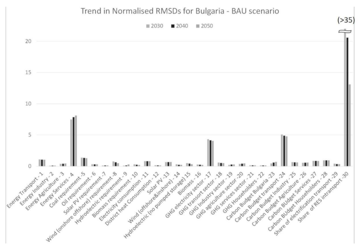
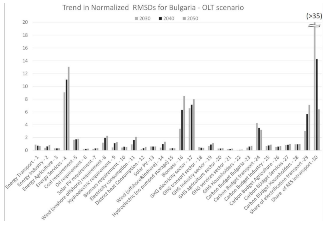
Comparing the series in normalized RMSDs values (Table 9 and Table 10), it is possible to explore the difference across the whole series of variables in BAU (Figure 5) and OLT (Figure 6) scenarios.
The variable 30 “Share of RES in transport” in the BAU scenario is influenced by the previous explained different approach between MEDEAS and LEAP in achieving decarbonization switching to RES; this provokes an increase in the share of electricity for transportation in 2020 even in a BAU perspective; this also affects the variable 24, the carbon budget accounts for transport and the GHG electricity sector (variable 17).
The variance in variable 4, energy for the service sector, is also due to the different approach of the two models: In MEDEAS, the final energy demands by final fuel necessary to produce a certain amount of goods and services is constrained by the available final energy that accounts for limitations of nonrenewable fuels—peak oil phenomena—and the sustainable potential of renewables, while this demand is not constrained in LEAP_bg.
The variance due to this limitation is emphasized in RMSDs (Table 10) evaluation for OLT scenarios (Figure 6). In OLT, biomass production faces the increase necessary to provide biofuels for transport: the LEAP unconstrained demand for biomass is much higher than the MEDEAS one.
Nevertheless, the simulated carbon budgets with MEDEAS_bg and LEAP_bg in OLT scenario are of the same order of magnitude, even this is higher than the estimated national objective of 1.45 GtCO2 eq, suggesting that further measures than RE implementations are necessary to meet the Paris target.
Similarly, to the case of Austria and TIMES, there are more similarities between MEDEAS_bg and LEAP_bg in designing the BAU scenarios than in designing OLT.

4. Discussion

Today, several IAMs coexist to deal with the complex interactions, high uncertainties, and knowledge gaps between interconnections within the environment and human societies [32,33,34]. For these reasons, it is usually quite challenging to compare IAMs, with very different characteristics [5]. Moreover, these simulation tools do not consider the possibility to jointly analyze the resource limitations, the impact of climate, and the feedbacks with the environment; besides, they are mainly world models with no geographical disaggregation of the economic evolution at lower geographical levels. The MEDEAS suite of models, not only fills those gaps for the world level but, due to its nested structure, also allows for exploring the global effect at regional and national levels. These are unprecedent features among the existing IAMs and the comparison of MEDEAS models with existing models [22] opens a new field of investigation to assess the efficiency of models in representing socio/ecological/economic dynamics of a country. For instance, some of the feedback loops of the MEDEAS models have to be turned off to allow for a realistic comparison with the traditional national models including TIMES and LEAP: this helps in making the two approaches comparable, but on the other side, the geographical upper-level variables and assumptions that may affect regional dynamics have not been included in the analysis, meaning that only partial conclusions on cross-validating MEDEAS country with a benchmark can be achieved at the present stage of investigation.
Nevertheless, extremely interesting findings can be highlighted from this study. One clear distinction from the cross-comparison and qualitative evaluation between MEDEAS country and TIMES-Austria and LEAP-Bulgaria highlight the approach used to simulate limited availability of natural resources: In MEDEAS, energy is not generated within the energy system, but it is converted into a usable form by technologies and is provided by a limited amount of available fossil resources. TIMES_at and LEAP_bg do not account for the limited availability of fossil fuels.
Moreover, MEDEAS can provide more comprehensive simulations by allowing disequilibrium dynamics in the economy by not assuming clearing markets (i.e., not imposing general equilibrium) [35], by including the evaluation of the effects of climate change on the economy [36] and the effects of (economic) development on depletion of natural resources [37], all in the context of simulations for the transition to a decarbonized energy system. Although other general equilibrium models like TIMES-Austria and LEAP-Bulgaria do not account for these dynamics, these models still provide invaluable information for infrastructure, investment, and capacity requirements for the transition, especially when specified at the national level.
TIMES_at was developed to create medium to long-term scenarios for the Austrian energy system. The optimization is conducted according to several constraints that are built into the model and can be parameterized. Crucially, in the TIMES model, energy demand development is to a large extent the result of exogenous scenario parameters including, most importantly, GDP growth and population growth. These parameters need to be assumed or modeled within a different framework. In MEDEAS, growth is exogenous only until energy limits are reached (if reached). Notably, there is no feedback from the energy system to GDP within TIMES, which has implications for scenario transition rate comparisons.
The system boundaries of the TIMES model include the Austrian energy system, structured into several sectors (industry, households, agriculture, electricity, and district heat supply etc.). To allow for direct and easy comparison with historical data, the structure of the model and model results is largely consistent with Austrian energy statistics. TIMES includes several assumptions that have implications for the results. First, TIMES assumes perfect foresight, which means that all investment decisions are made in each period with full knowledge of future events (fuel price developments, technologies available in the future, etc.).
LEAP_bg is an integrated, scenario-based modeling tool that accounts for both energy sector and non-energy sector greenhouse gas (GHG) emission sources and sinks [20]. The LEAP modeling procedure asks for specifying of key non-energy assumptions (demographic, macroeconomic, etc.), energy demand and energy supply, energy losses, own needs, exogenous and endogenous production capacities, import/export, so that LEAP_bg calculates the necessary energy production (to cover the demand, losses, etc.), additional capacities needed, primary energy requirements, emissions, and costs.

5. Conclusions

In the present study, we compared the results of the MEDEAS country models for Austria and Bulgaria with those of existing country-level models, TIMES and LEAP, used by Austrian Energy Agency and the Black Sea Energy Research Center of Bulgaria, with the aim to draft preliminary guidelines in validating a completely new modeling approach, the MEDEAS IAM at the regional level.
The main difference between MEDEAS and the other models is the innovative approach implemented in the development of MEDEAS, especially as regarding the modeling of the economy (non-clearing markets) and the environmental and biophysical constraints introduced and, most importantly, the connection between the two. TIMES-Austria and LEAP-Bulgaria being more focused on the components of the energy system and in optimizing, minimizing, or maximizing energy functions undoubtedly put more emphasis on detailed simulations for specific geographical areas. MEDEAS is instead focused on simulating dynamics and interactions within the energy system and its dependencies and interactions with other social-environmental systems.
Regarding quantitative evaluations, the models’ outputs compared are those generated simulating two long term scenarios: the business as usual (BAU) and optimal level transition (OLT) scenarios, each one adapted to Austria and Bulgaria respective energy–economy–environment structures. The BAU scenario assumes the future evolves following historical trends, while, OLT represents a scenario of economic growth and reduction of energy use through improvements in energy efficiency and implementing renewable energy, to accomplish national decarbonization according to the goals of the Paris Agreement.
As for the results from the normalizations of the TIMES and LEAP data series in respect to the MEDEAS series mean values (within each dataset), the RMSDs show that correlations between the models and across all the variables are higher for BAU scenarios in comparing MEDEAS_at with TIMES_at and also for MEDEAS_bg versus LEAP_bg. However, the highers RMSDs in OLT scenarios are mainly traceable to the models’ conception and structure differences rather than in a real mismatch in representing the same scenarios.

Author Contributions

Conceptualization, I.P. and G.M.; methodology, R.S.; software, G.M.; validation, A.N., L.E. and M.B.; formal analysis, G.M., A.J.; investigation, R.S., A.N., L.E.; resources, A.N., M.B., D.N.; data curation, I.P., A.N. and L.E.; writing—original draft preparation, I.P. and D.N.; writing—review and editing, R.S. A.J. and J.S.; supervision, U.B.; project administration, J.S.; funding acquisition, J.S. All authors have read and agreed to the published version of the manuscript.

Funding

This work was supported by the MEDEAS project, funded by the European Union’s Horizon 2020 research and innovation program under grant agreement No 691287. The opinion expressed in the present work are those of the authors’ only and are not to be attributed to any organization of the European Union.

Institutional Review Board Statement

Not Applicable.

Informed Consent Statement

Not Applicable.

Data Availability Statement

Restrictions apply to the availability of these data. Data was obtained from AEA and BSERC and are available from the authors with the permission of AEA and BSERC.

Conflicts of Interest

The authors declare no conflict of interest.

Appendix A. Evaluation of National Carbon Budget for Austria and Bulgaria

The EU carbon budget of 122 GtCO2 eq evaluated in the previous study of Perissi and others [27] was split for each of the EU28 countries on the base of their historical emission trends, with the final aim to evaluate a national carbon budget for Austria and Bulgaria in the frame of the EU28 policy and the COP21 policy. These carbon budgets are used to define OLTs scenarios that aim to attain the energy transition while minimizing the emissions at the country level.
We briefly recall here that the evaluation of country-level carbon budgets has been carried out by projecting EU countries GHG emissions by sectors to 2100, considering in that year, each EU28 country should be completely decarbonized. The projections are shaped as follow: linear extrapolation of sectors’ GHG historical trends (source Eurostat) to 2020, then we considered a power decay to the final emissions values in 2100 (which are zero, considering, as mentioned before, an EU 28 total decarbonization).
Moreover, only for the power sectors, we assumed it will be completely decarbonized already in 2050, as the more urgent target to achieve, enabling, in consequence, faster decarbonization of the other sectors (i.e., electric transportation). For the rest of the sectors, any emissions target was established in 2050, letting each country to act with more degrees of freedom across the nonpower sectors in achieving their decarbonization. As a starting point for historical trends extrapolation, we set the year 2005. Renewables energy started to be on the market, as a tangible alternative to fossil fuels, around 2004 (source Eurostat):
Applying the above procedure, for the OLT 2020 Austria we found an estimation of the national carbon budget of about 1.85 GtCO2 eq (Figure A1).
The obtained value is comparable with the study from the Universitat Politecnica de Catalunya—Grup sobre Government del Canvi Climàtic (Grup sobre Governament del Canvi Climàtic, 2015), which is based on the assumption of RCP 2.6 scenarios that admit a global annual GHG emissions (measured in CO2 eq) peak between 2010–2020, with emissions declining substantially thereafter. With this hypothesis, GGCC estimates for Austria a carbon budget around 1.8 GtCO2 eq.
Figure A1. 2020 Austria economic sectors’ emissions scenario. Possible pathways for the country decarbonization, according to the recommendations from the EU 2050 Roadmap and the COP21 constraint on global warming.
Sustainability 13 01967 g0a1
Applying the same procedure adopted for the case of Austria, the OLT 2020 Bulgaria results in an estimation of the national carbon budget of about 1.45 GtCO2 eq (Figure A2).
The obtained value is slightly higher than the one from the study of the Universitad Politecnica de Catalunya (Grup sobre Governament del Canvi Climàtic, 2015), which is based on the assumption of RCP 2.6 scenarios that admit a global annual GHG emissions (measured in CO2 eq) peak between 2010–2020, with emissions declining substantially thereafter. With this hypothesis, GGCC estimates for Bulgaria a carbon budget around 1.2 GtCO2 eq.
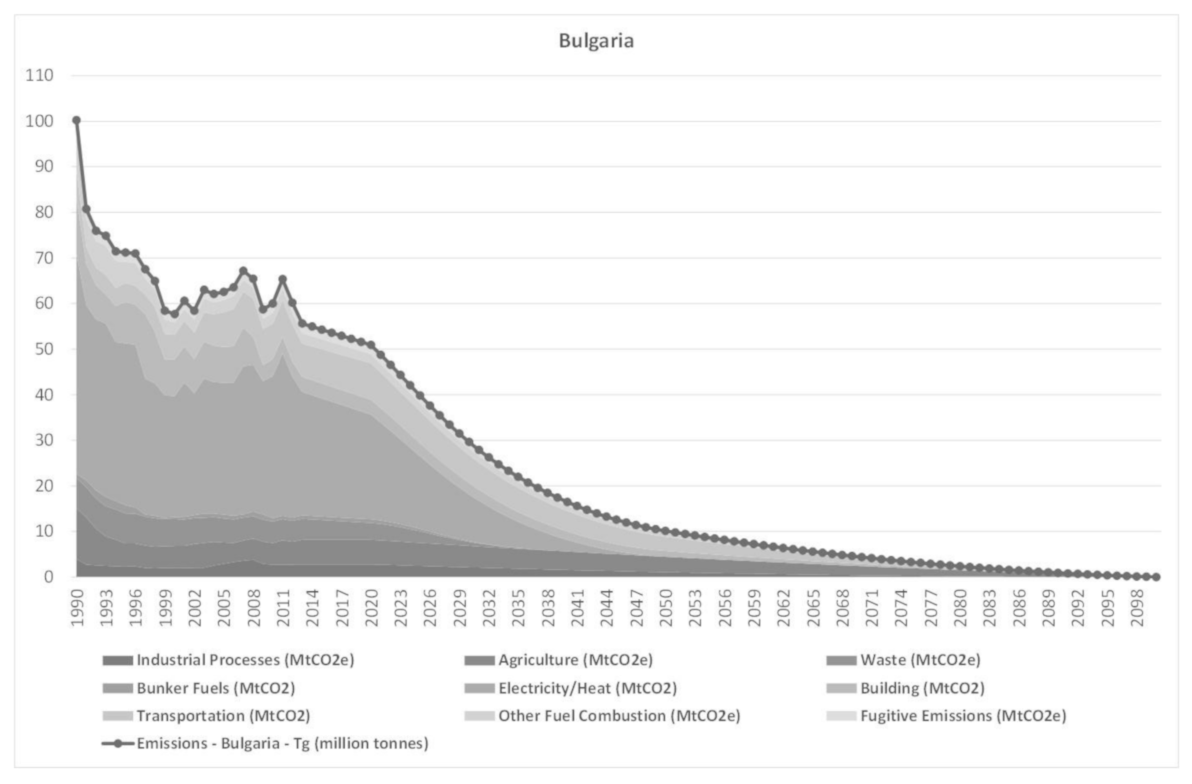
Figure A2. 2020 Bulgaria economic sectors’ emissions scenario. Possible pathways for the country decarbonization, according to the recommendations from the EU 2050 Roadmap and the COP21 constraint on global warming.
Sustainability 13 01967 g0a2

Appendix B

Appendix B.1. MATLAB CODE Austria Normalized RMSD

clear
close all
RMSD1=[];
RMSD2=[];
M1=xlsread(’CCV1.xlsx’,’1 BAU’); % reading sheet "1 BAU"
M2=xlsread(’CCV1.xlsx’,’2 OLT’); % reading sheet "2 OLT"
S1=size(M1); % number of row and column sheet "1 BAU" data S2=size(M2); % number of row and column sheet sheet "2 OLT" data C1=S1(2); % number of column sheet "1 BAU" data
C2=S2(2); % number of column sheet "2 OLT" data
time_years1=M1(1,1:C2); % row of temporal axis in year sheet "1 BAU"
time_years2=M2(1,1:C2); % row of temporal axis in year sheet "2 OLT"
f=4; % repeated data each 4 rows
I1=S1(1)/f; % number of row couples (to compare) for calculating RMSD sheet "1 BAU"
I2=S2(1)/f; % % number of row couples (to compare) for calculating RMSD sheet "2 OLT"
for dt=0:5:25 % 0=2050, 5=2045, 10=2040, 15=2035, 20=2030, 25=2025
rmsd1=zeros(1,I1); % memory allocation for rmsd vector (sheet "1 BAU")
rmsd2=zeros(1,I2); % memory allocation for rmsd vector (sheet "2 OLT")
% Calculus on sheet "1 BAU"
M_data1=zeros(I1,C2); % Medeas model data memory allocation
T_data1=zeros(I1,C2); % Times model data memory allocation
DIFN=zeros(I1,C2); % time error memory allocation
for i=1:I1
if i<I1
M_data1(i,:)=M1(f*(i-1)+3,1:C2); % Medeas model data
T_data1(i,:)=M1(f*i,1:C2)/10^6; % Times model data
DIF=M_data1(i,1:end-dt)-T_data1(i,1:end-dt);
rmsd1(i)=(1/(mean(M_data1(i,1:end-dt))))*sqrt(sum(DIF.^2)/(1+time_years1(end-dt)-time_years1(1))); % rmsd computation
DIFN(i,1:end-dt)=DIF;
else% last two rows in % (not energy => not division per 10^6) M_data1(i,:)=M1(f*(i-1)+3,1:C2); % Medeas model data
T_data1(i,:)=M1(f*i,1:C2); % Times model data
DIF=M_data1(i,1:end-dt)-T_data1(i,1:end-dt);
rmsd1(i)=(1/(mean(M_data1(i,1:end-dt))))*sqrt(sum(DIF.^2)/(1+time_years1(end-dt)-time_years1(1))); % rmsd computation
DIFN(i,1:end-dt)=DIF;
end
end
rmsd1=rmsd1(~isnan(rmsd1));
RMSD1=[RMSD1;rmsd1];
% Calculus on sheet "2 OLT"
M_data2=zeros(I2,C2); % Medeas model data memory allocation
T_data2=zeros(I2,C2); % Times model data memory allocation
DIFN2=zeros(I2,C2); % time error memory allocation
for i=1:I2
if i<I2
M_data2(i,:)=M2(f*(i-1)+3,1:C2); % Medeas model data
T_data2(i,:)=M2(f*i,1:C2)/10^6; % Times model data
DIF2=M_data2(i,1:end-dt)-T_data2(i,1:end-dt);
rmsd2(i)=(1/(mean(M_data2(i,1:end-dt))))*sqrt(sum(DIF2.^2)/(1+time_years2(end-dt)-time_years2(1))); % rmsd computation
DIFN2(i,1:end-dt)=DIF2;
else% last two rows in % (not energy => not division per 10^6) M_data2(i,:)=M2(f*(i-1)+3,1:C2); % Medeas model data
T_data2(i,:)=M2(f*i,1:C2); % Times model data
DIF2=M_data2(i,1:end-dt)-T_data2(i,1:end-dt);
rmsd2(i)=(1/(mean(M_data2(i,1:end-dt))))*sqrt(sum(DIF2.^2)/(1+time_years2(end-dt)-time_years2(1))); % rmsd computation
DIFN2(i,1:end-dt)=DIF2;
end
end
rmsd2=rmsd2(~isnan(rmsd2));
RMSD2=[RMSD2;rmsd2];
% two sheets rmsd plot
figure(1+2*dt/5)
plot(rmsd1,‘ob’)
xlabel(‘# parameters’)
ylabel(‘RMSD’)
title(‘RMSD sheet BAU’)
grid on
figure(2+2*dt/5)
plot(rmsd2,‘or’)
xlabel(‘# parameters’)
ylabel(‘RMSD’)
title(‘RMSD sheet OLT’)
grid on
end
RMSD1=[(2050:-5:2025)’,RMSD1];
RMSD2=[(2050:-5:2025)’,RMSD2];

Appendix B.2. MATLAB CODE Bulgaria Normalized RMSD

clear
close all
RMSD1=[[];
RMSD2=[[];
M1=xlsread(’CCV2.xlsx’,’1 BAU’); % reading sheet "1 BAU"
M2=xlsread(’CCV2.xlsx’,’2 OLT’); % reading sheet "2 OLT"
S1=size(M1); % number of row and column sheet "1 BAU" data
S2=size(M2); % number of row and column sheet sheet "2 OLT" data
C1=S1(2); % number of column sheet "1 BAU" data
C2=S2(2); % number of column sheet "2 OLT" data
time_years1=M1(1,1:C1); % row of temporal axis in year sheet "1 BAU"
time_years2=M2(1,1:C2); % row of temporal axis in year sheet "2 OLT"
f=4; % repeated data each 4 rows
I1=(S1(1)+1)/f; % number of row couples (to compare) for calculating RMSD sheet "1 BAU"
I2=(S2(1)-2)/f; % number of row couples (to compare) for calculating RMSD sheet "2 OLT"
for dt=0:5:25 % 0=2050, 5=2045, 10=2040, 15=2035, 20=2030, 25=2025
rmsd1=zeros(1,I1); % memory allocation for rmsd vector (sheet "1 BAU")
rmsd2=zeros(1,I2); % memory allocation for rmsd vector (sheet "2 OLT")
% Calculus on sheet "1 BAU"
L_data1=zeros(I1,C1); % Leap model data memory allocation
M_data1=zeros(I1,C1); % Medeas model data memory allocation
DIFN=zeros(I1,C1); % time error memory allocation
for i=1:I1
if i<=I1-14
L_data1(i,:)=M1(f*(i-1)+2,1:C1)/10^6; % Leap model data
M_data1(i,:)=M1(f*(i-1)+3,1:C1); % Medeas model data
DIF=M_data1(i,1:end-dt)-L_data1(i,1:end-dt);
rmsd1(i)=(1/(mean(M_data1(i,1:end-dt))))*sqrt(sum(DIF.^2)/(1+time_years1(end-dt)-time_years1(1))); % rmsd computation
DIFN(i,1:end-dt)=DIF;
elseif i>I1-14 && i<=I1-8
L_data1(i,:)=M1(f*(i-1)+2,1:C1)/1000; % Leap model data (conversion from PJ to EJ)
M_data1(i,:)=M1(f*(i-1)+3,1:C1); % Medeas model data
DIF=M_data1(i,1:end-dt)-L_data1(i,1:end-dt);
rmsd1(i)=(1/(mean(M_data1(i,1:end-dt))))*sqrt(sum(DIF.^2)/(1+time_years1(end-dt)-time_years1(1))); % rmsd computation
DIFN(i,1:end-dt)=DIF;
elseif i>I1-8 && i<I1-1
L_data1(i,:)=M1(f*(i-1)+2,1:C1)*4.184/1000; % Leap model data(conversion from MT to EJ)
M_data1(i,:)=M1(f*(i-1)+3,1:C1); % Medeas model data
DIF=M_data1(i,1:end-dt)-L_data1(i,1:end-dt);
rmsd1(i)=(1/(mean(M_data1(i,1:end-dt))))*sqrt(sum(DIF.^2)/(1+time_years1(end-dt)-time_years1(1))); % rmsd computation
DIFN(i,1:end-dt)=DIF;
else% last two rows in % (not energy => not division per 10^6)
L_data1(i,:)=M1(f*(i-1)+2,1:C1); % Leap model data
M_data1(i,:)=M1(f*(i-1)+3,1:C1); % Medeas model data
DIF=M_data1(i,1:end-dt)-L_data1(i,1:end-dt);
rmsd1(i)=(1/(mean(M_data1(i,1:end-dt))))*sqrt(sum(DIF.^2)/(1+time_years1(end-dt)-time_years1(1))); % rmsd computation
DIFN(i,1:end-dt)=DIF;
end
end
rmsd1=rmsd1(~isnan(rmsd1));
RMSD1=[RMSD1;rmsd1];
% Calculus on sheet "2 OLT"
L_data2=zeros(I2,C2); % Leap model data memory allocation
M_data2=zeros(I2,C2); % Medeas model data memory allocation
DIFN2=zeros(I1,C1); % time error memory allocation
for i=1:I2
if i<=I2-14
L_data2(i,:)=M2(f*(i-1)+5,1:C2)/10^6; % Leap model data
M_data2(i,:)=M2(f*i+2,1:C2); % Medeas model data
DIF2=M_data2(i,1:end-dt)-L_data2(i,1:end-dt);
rmsd2(i)=(1/(mean(M_data2(i,1:end-dt))))*sqrt(sum(DIF2.^2)/(1+time_years2(end-dt)-time_years2(1))); % rmsd computation
DIFN2(i,1:end-dt)=DIF2;
elseif i>I2-14 && i<=I2-8
L_data2(i,:)=M2(f*(i-1)+5,1:C2)/1000; % Leap model data (conversion from PJ to EJ)
M_data2(i,:)=M2(f*i+2,1:C2); % Medeas model data
DIF2=M_data2(i,1:end-dt)-L_data2(i,1:end-dt);
rmsd2(i)=(1/(mean(M_data2(i,1:end-dt))))*sqrt(sum(DIF2.^2)/(1+time_years2(end-dt)-time_years2(1))); % rmsd computation
DIFN2(i,1:end-dt)=DIF2;
elseif i>I2-8 && i<I2-1
L_data2(i,:)=M2(f*(i-1)+5,1:C2)*4.184/1000; % Leap model data (conversion from MT to EJ)
M_data2(i,:)=M2(f*i+2,1:C2); % Medeas model data
DIF2=M_data2(i,1:end-dt)-L_data2(i,1:end-dt);
rmsd2(i)=(1/(mean(M_data2(i,1:end-dt))))*sqrt(sum(DIF2.^2)/(1+time_years2(end-dt)-time_years2(1))); % rmsd computation
DIFN2(i,1:end-dt)=DIF2;
else% last two rows in % (not energy => not division per 10^6)
L_data2(i,:)=M2(f*(i-1)+5,1:C2); % Leap model data
M_data2(i,:)=M2(f*i+2,1:C2); % Medeas model data
DIF2=M_data2(i,1:end-dt)-L_data2(i,1:end-dt);
rmsd2(i)=(1/(mean(M_data2(i,1:end-dt))))*sqrt(sum(DIF2.^2)/(1+time_years2(end-dt)-time_years2(1))); % rmsd computation
DIFN2(i,1:end-dt)=DIF2;
end
end
rmsd2=rmsd2(~isnan(rmsd2));
RMSD2=[RMSD2;rmsd2];
% two sheets rmsd plot
figure(1+2*dt/5)
plot(rmsd1,‘ob’)
xlabel(‘# parameters’)
ylabel(‘RMSD’)
title(‘RMSD sheet BAU’)
grid on
figure(2+2*dt/5)
plot(rmsd2,‘or’)
xlabel(‘# parameters’)
ylabel(‘RMSD’)
title(‘RMSD sheet OLT’)
grid on
end
RMSD1=[(2050:-5:2025)’,RMSD1];
RMSD2=[(2050:-5:2025)’,RMSD2];

References

  1. Rotmans, J.; van Asselt, M.B.A. Uncertainty in Integrated Assessment Modelling: A Labyrinthic Path. Uncertain. Integr. Assess. Model. Labyrinthic Path 2001, 2, 43–55. [Google Scholar] [CrossRef]
  2. Pfenninger, S.; De Carolis, J.; Hirth, L.; Quoilin, S.; Staffell, I. The importance of open data and software: Is energy research lagging behind? Energy Policy 2017, 101, 211–215. [Google Scholar] [CrossRef]
  3. Meadows, D.H.M. The Limits to Growth. Club Rome 1972, 211. [Google Scholar] [CrossRef]
  4. Hafner, S.; Anger-Kraavi, A.; Monasterolo, I.; Jones, A. Emergence of New Economics Energy Transition Models: A Review. Ecol. Econ. 2020, 177, 106779. [Google Scholar] [CrossRef]
  5. Capellán-Pérez, I.; de Blas, I.; Nieto, J.; de Castro, C.; Miguel, L.J.; Carpintero, Ó.; Mediavilla, M.; Lobejón, L.F.; Ferreras-Alonso, N.; Rodrigo, P.; et al. MEDEAS: A new modeling framework integrating global biophysical and socioeconomic constraints. Energy Environ. Sci. 2020, 13, 986–1017. [Google Scholar] [CrossRef]
  6. Scrieciu, S.; Rezai, A.; Mechler, R. On the economic foundations of green growth discourses: The case of climate change mitigation and macroeconomic dynamics in economic modeling: Economic foundations of green growth discourses. Wiley Interdiscip. Rev. Energy Environ. 2013, 2, 251–268. [Google Scholar] [CrossRef]
  7. Diaz, D.; Moore, F. Quantifying the economic risks of climate change. Nat. Clim. Chang. 2017, 7, 774–782. [Google Scholar] [CrossRef]
  8. Dietz, S.; Stern, N. Endogenous Growth, Convexity of Damage and Climate Risk: How Nordhaus’ Framework Supports Deep Cuts in Carbon Emissions. Econ. J. 2015, 125, 574–620. [Google Scholar] [CrossRef] [Green Version]
  9. Ringkjøb, H.-K.; Haugan, P.M.; Solbrekke, I.M. A review of modelling tools for energy and electricity systems with large shares of variable renewables. Renew. Sustain. Energy Rev. 2018, 96, 440–459. [Google Scholar] [CrossRef]
  10. Solé, J.; Samsó, R.; García-Ladona, E.; García-Olivares, A.; Ballabrera-Poy, J.; Madurell, T.; Turiel, A.; Osychenko, O.; Álvarez, D.; Bardi, U.; et al. Modelling the renewable transition: Scenarios and pathways for a decarbonized future using pymedeas, a new open-source energy systems model. Renew. Sustain. Energy Rev. 2020, 132, 110105. [Google Scholar] [CrossRef]
  11. Capellán-Pérez, I.; de Castro, C.; Miguel González, L.J. Dynamic Energy Return on Energy Investment (EROI) and material requirements in scenarios of global transition to renewable energies. Energy Strategy Rev. 2019, 26, 100399. [Google Scholar] [CrossRef]
  12. Martelloni, G.; Falsini, S.; Di Patti, F.; Bardi, U. MEDEAS-World Model Calibration for the Study of the Energy Transition. PuntOorg Int. J. 2020, 4, 119–140. [Google Scholar] [CrossRef] [Green Version]
  13. De Blas, I.; Miguel, L.J.; Capellán-Pérez, I. Modelling of sectoral energy demand through energy intensities in MEDEAS integrated assessment model. Energy Strategy Rev. 2019, 26, 100419. [Google Scholar] [CrossRef]
  14. MEDEAS. MEDEAS Project. Modelling the Energy Development under Environmental And Socioeconomic Constraints. 2019. Available online: www.medeas.eu (accessed on 10 February 2021).
  15. Solé, J.; García-Olivares, A.; Turiel, A.; Ballabrera-Poy, J. Renewable transitions and the net energy from oil liquids: A scenarios study. Renew. Energy 2018, 116, 258–271. [Google Scholar] [CrossRef]
  16. Capellán-Pérez, I.; De Blas, I.; Nieto, J.; De Castro, C.; Miguel, L.J.; Mediavilla, M.; Carpintero, O.; Rodrigo, P.; Frechoso, F.; Cáceres, S. Modelling Sustainable Energy System Development under Environmental and Socioeconomic Constraints; MEDEAS scenarios Deliverable D4.1; MEDEAS: Pleasanton, CA, USA, 2017. [Google Scholar]
  17. UNEP. Decoupling Natural Resource Use and Environmental Impacts from Economic Growth; UNEP: Nairobi, Kenya, 2011. [Google Scholar]
  18. Loulou, R. Documentation for the MARKAL Family of Models. Energy Technol. Syst. Anal. Programme 2004, 389, 65–73. [Google Scholar]
  19. Loulou, R.; Remne, U.; Kanudia, A.; Lehtila, A.; Goldstein, G. Documentation for the TIMES Model—PART 1. IEA Energy Technol. Syst. Anal. Programme 2005, 1, 1–78. [Google Scholar]
  20. Heaps, Charles Long-Range Energy Alternatives Planning (LEAP) System. [software version: 2020.1.20]. Stockholm Environment Institute: Somerville, MA, USA. Available online: https://leap.sei.org (accessed on 10 February 2021).
  21. Connolly, D.; Lund, H.; Mathiesen, B.V.; Leahy, M. A review of computer tools for analysing the integration of renewable energy into various energy systems. Appl. Energy 2010, 87, 1059–1082. [Google Scholar] [CrossRef]
  22. Van Beeck, N.M.J.P. Classification of Energy Models; FEW Research Memorandum; Operations research: Tilburg, The Netherlands, 1999; Volume 777. [Google Scholar]
  23. «MEDEAS Models Cross Validation», MEDEAS. 2019. Available online: https://www.medeas.eu/model/medeas-vs-times-leap (accessed on 10 February 2021).
  24. Nieto, J.; Carpintero, Ó.; Miguel, L.J.; de Blas, I. Macroeconomic modelling under energy constraints: Global low carbon transition scenarios. Energy Policy 2020, 137, 111090. [Google Scholar] [CrossRef] [Green Version]
  25. Samsó, R.; de Blas, I.; Perissi, I.; Martelloni, G.; Solé, J. Scenario analysis and sensitivity exploration of the MEDEAS Europe energy-economy-environment model. Energy Strategy Rev. 2020, 100582. [Google Scholar] [CrossRef]
  26. United Nations Paris Agreement. 2015. Available online: http://unfccc.int/paris_agreement/items/9485.php (accessed on 9 February 2021).
  27. Perissi, I.; Falsini, S.; Bardi, U.; Natalini, D.; Green, M.; Jones, A.; Sol, J. Potential European Emissions Trajectories within the Global Carbon Budget. Sustainability 2018, 10, 4225. [Google Scholar] [CrossRef] [Green Version]
  28. Myung, I.J. The Importance of Complexity in Model Selection. J. Math. Psychol. 2000, 44, 190–204. [Google Scholar] [CrossRef] [Green Version]
  29. Hyndman, R.J.; Koehler, A.B. Another look at measures of forecast accuracy. Int. J. Forecast. 2006, 22, 679–688. [Google Scholar] [CrossRef] [Green Version]
  30. McVicar, T. Estimating one-time-of-day meteorological data from standard daily data as inputs to thermal remote sensing based energy balance models. Agric. For. Meteorol. 1999, 96, 219–238. [Google Scholar] [CrossRef]
  31. Zambrensky, L. A Verification Study of the Global WAM Model; technical report no. 63 1987; ECMWF: Shinfield Park, UK, 1989. [Google Scholar]
  32. Siegenfeld, A.F.; Bar-Yam, Y. An Introduction to Complex Systems Science and Its Applications. Complexity 2020, 2020, 6105872. [Google Scholar] [CrossRef]
  33. Bardi, U.; Falsini, S.; Perissi, I. Toward a General Theory of Societal Collapse. A Biophysical Examination of Tainter’s Model of the Diminishing Returns of Complexity. Biophys. Econ. Resour. Qual. 2018, arXiv:1810.07056. [Google Scholar] [CrossRef] [Green Version]
  34. Barabási, A.-L. Scale-Free Networks: A Decade and Beyond. Science 2009, 325, 412–413. [Google Scholar] [CrossRef] [Green Version]
  35. Nieto, J.; Carpintero, Ó.; Lobejón, L.F.; Miguel, L.J. An ecological macroeconomics model: The energy transition in the EU. Energy Policy 2020, 145, 111726. [Google Scholar] [CrossRef]
  36. Nieto, J.; Carpintero, Ó.; Miguel, L.J. Less than 2 °C? An Economic-Environmental Evaluation of the Paris Agreement. Ecol. Econ. 2018, 146, 69–84. [Google Scholar] [CrossRef]
  37. Valero, A.; Valero, A.; Calvo, G.; Ortego, A. Material bottlenecks in the future development of green technologies. Renew. Sustain. Energy Rev. 2018, 93, 178–200. [Google Scholar] [CrossRef]
Figure 1. Overview of MEDEAS by modules and the modeled linkages between them. Interrelations between the 7 modules: The main variables that connect the different modules are represented by arrows. Most modules have bi-directional linkages, excepting for the Land Use and Social and Environmental impacts indicators which mainly report outputs from the simulations without feed-backing to the rest of the structure.
Sustainability 13 01967 g001
Figure 2. Business as Usual (BAU) and Optimal Level Transition (OLT) scenarios of the energy consumption in the industry sector in Austria and Bulgaria evaluated with MEDEAS countries and the national models TIMES_at (a,b) and LEAP_bg (c,d).
Sustainability 13 01967 g002
Figure 3. Plot of the normalized RMSDs distribution for the cross-validation of MEDEAS_at vs. TIMES_at, for BAU scenarios (BAU_at_norm). Normalized RMSDs series were calculated between 2010–2030; 2010–2040; 2010–2050 to evaluate how RMSDs evolve with time.
Sustainability 13 01967 g003
Figure 4. Plot of the normalized RMSDs distribution for the cross-validation of MEDEAS_at vs. TIMES_at in OLT scenario. Normalized RMSDs series were calculated between 2010–2030; 2010–2040; 2010–2050 to evaluate how RMSDs evolve with time.
Sustainability 13 01967 g004
Figure 5. Plot of the normalized RMSDs distribution values for the BAU_bg for the cross-validation of MEDEAS_bg vs. LEAP_bg.
Sustainability 13 01967 g005
Figure 6. Comparison of the number of variables as a function of normalized RMSD for MEDEAS_bg and LEAP_bg in the OLT scenario.
Sustainability 13 01967 g006
Table 1. List of common outputs of the MEDEAS_at and TIMES-at analyzed in cross-validation. The nomenclature used here for the output variables names is the Vensim system for MEDEAS countries and The Integrated MARKAL-EFOM System TIMES model nomenclature for TIMES Austria.
SECTORSMEDEAS_atTIMES_at
1Electricity sectorReal final energy by sector and fuel AUT [scenarios, final sources! Electricity Gas and Water Supply]Export-Ver brauch Sektor Energie
2Transport sectorReal final energy by sector and fuel AUT [scenarios, final sources! TRANSPORT SECTORS!]Export-EEV by Sector-en [transport]
3IndustryReal final energy by sector and fuel AUT [scenarios, final sources! INDUSTRY SECTORS!]Export-EEV by Sector-en [industry]
4AgricultureReal final energy by sector and fuel AUT [scenarios, final sources! agriculture hunting forestry and fishing]Export-EEV by Sector-en [agriculture]
5Natural gasPES fossil fuel extraction [scenarios, gases]Export-BIV-en [gas]
6CoalPES fossil fuel extraction [scenarios, solids]Export-BIV-en [coal]
7OilPES fossil fuel extraction [scenarios, liquids]Export-BIV-en [oil]
8Solar PVPE solar PV for Elec generation EJ [scenarios]Export-BIV-en [solar PV]
9HydroelectricPE hydro for Elec generation EJ [scenarios]Export-BIV-en [hydro]
10BiomassPE bioE for Elec generation EJ [scenarios]Export-BIV-en [biomass]
11Heatreal FE consumption by fuel [scenarios, heat]Export-EEV-total-agg-en [heat]
12Electricityreal FE consumption by fuel [scenarios, electricity]Export-EEV-total-agg-en [Elec]
13Solar PVinstalled capacity RES elec TW [solar PV, scenarios]Export-ELC-Cap-Ty [solar PV]
14Wind (inshore)installed capacity RES elec TW [wind onshore, scenarios]Export-ELC-Cap-Ty [windOn]
15Hydroelectric excl. Pumped storageinstalled capacity RES elec TW [hydro, scenarios]Export-ELC-Cap-Ty [hydro]
16Biomassinstalled capacity RES elec TW [“solid bioE-elec”, scenarios]Export-ELC-Cap-Ty [solid Bio-e]
17Electricity sectorGHG emissions by FE Electricity sector [scenarios, final sources]Export-GHG-perTH GSektor-en [elecricity]
18Transport sectorGHG emissions by FE Transport sector [scenarios, final sources]Export-GHG-perTH GSektor-en [transport]
19Industry sectorGHG emissions by FE Industry sector [scenarios, final sources]Export-GHG-perTH GSektor-en [industry]
20Agriculture sectorGHG emissions by FE Agriculture sector [scenarios, final sources]Export-GHG-perTH GSektor-en [agriculture]
21Services sectorGHG emissions by FE Services sector [scenarios, final sources]Export-GHG-perTH GSektor-en [services]
22Household sectorGHG emissions by FE Households sector [scenarios, final sources]Export-GHG-perTHG-en [households]
23Share of electrification of transport sectorShare demand electricity in transport [scenarios]Export-Transport-EEV-total-en [transport]
Table 2. List of common outputs of the MEDEAS_bg and LEAP_bg analyzed in cross-validation. The nomenclature used here for the output variables names is the Vensim models ones for MEDEAS countries and the Long-Range Energy Alternatives Planning System (LEAP) nomenclature for LEAP Bulgaria.
SECTORSMEDEAS_bgLEAP_bg
1Transport sectorReal final energy by sector and fuel BGR [BAU, transport]Energy demand final units: Transport
2Industry sectorReal final energy by sector and fuel BGR [BAU, industry]Energy demand final units: Industry
3Agriculture sectorReal final energy by sector and fuel BGR [BAU, agriculture]Energy demand final units: Agriculture
4Services sectorReal final energy by sector and fuel BGR [BAU, services]Energy demand final units: Services
5CoalPES fossil fuel extraction [BAU, solids]Primary requirements/Coal Antracite + Coal Lignite + Coke
6OilPES fossil fuel extraction [BAU, liquids]Primary requirements/Gasoline + Diesel + Jet Kerosine + Residual Fuel oil + LPG
7 PE solar PV for Elec generation EJ [BAU]Primary requirements/Solar (PV share)
8Wind (onshore and offshore)PE onshore wind for Elec generation EJ [BAU]Primary requirements/wind
9HydroelectricPE hydro for Elec generation EJ [BAU]Primary requirements/Hydro
10BiomassPE bioE for Elec generation EJ [BAU]Primary requirements/biomass + biogas + biodiesel + ethanol + MSW + charcoal
11Electricityreal FE consumption by fuel [BAU, electricity]FEC/electricity
12District heatreal FE consumption by fuel [BAU, heat]FEC/heat
13Solar PVinstalled capacity RES elec TW [solar PV]Capacity: PV
14Wind (onshore and offshore)installed capacity RES elec TW [wind onshore]Capacity: Wind
15Hydroelectric excl. Pumped storageinstalled capacity RES elec TW [hydro, scenarios]Capacity: Hydro (excl. PSP)
16Biomass (electric)installed capacity RES elec TW [“solid bioE-elec”, scenarios]Capacity: Biomass
17Electricity sectorGHG Electricity sector [scenarios]total = direct + indirect (heat and electricity emissions allocated to demand).
18Transport sectorGHG Transport sector [scenarios]
19Industry sectorGHG Industry sector [scenarios]
20Agriculture sectorGHG Agriculture sector [scenarios]
21Services sectorGHG Services sector [scenarios]
22Household sectorGHG Households sector [scenarios]
23Cumulative GHG emissions (million metric ton CO2 eq.)Cumulative CO2e GHG emissions [scenarios]Direct plus Indirect emissions (CO2e).
24Cumulative GHG Transport sectorGHG emissions by FE Transport sector [scenarios, final sources]Emissions allocated to demands: Transport
25Cumulative GHG Industry sectorGHG emissions by FE Industry sector [scenarios, final sources]Emissions allocated to demands: Industry
26Cumulative GHG Agriculture sectorGHG emissions by FE Agriculture sector [scenarios, final sources]Emissions allocated to demands: Agriculture
27Cumulative GHG Services sectorGHG emissions by FE Services sector [scenarios, final sources]Emissions allocated to demands: Services
28Cumulative GHG Household sectorGHG emissions by FE Households sector [scenarios, final sources]Emissions allocated to demands: Residential
29Share of electrification of transport sectorShare demand electricity in transport [scenarios]Share of electricity vs. Total
30Share of RES in transportationshare RES elect in transport [scenarios] + share RES liquids in transport [scenarios]Includes RES share in transport and RES share of the electricity in transport
Table 3. Standard Root Mean Square Differences (RMSDs) between MEDEAS_at and TIMES_at within the BAU_at scenario. RMSDs are calculated starting from the year 2010.
Austria SECTORS BAU_at Abs203020402050
1Electricity sector5.87 × 10−25.67 × 10−25.52 × 10−2
2Transport sector2.36 × 10−12.26 × 10−12.16 × 10−1
3Industry7.92 × 10−27.85 × 10−27.15 × 10−2
4Agriculture1.27 × 10−32.46 × 10−33.66 × 10−3
5Natural gas8.86 × 10−21.32 × 10−11.74 × 10−1
6Coal1.46 × 10−12.03 × 10−12.51 × 10−1
7Oil6.24 × 10−21.06 × 10−11.50 × 10−1
8Solar PV4.07 × 10−38.51 × 10−31.47 × 10−2
9Hydroelectric9.91 × 10−38.33 × 10−38.51 × 10−3
10Biomass1.93 × 10−11.93 × 10−11.90 × 10−1
11Heat3.10 × 10−13.35 × 10−13.64 × 10−1
12Electricity8.43 × 10−21.17 × 10−11.51 × 10−1
13Solar PV8.37 × 10−41.90 × 10−33.39 × 10−3
14Wind (inshore)8.47 × 10−41.95 × 10−32.96 × 10⁻³
15Hydroelectric excl. Pumped storage1.18 × 10−31.01 × 10−39.47 × 10−4
16Biomass1.21 × 10−31.16 × 10−31.16 × 10−3
17Electricity sector3.36 × 10−33.13 × 10−32.99 × 10−3
18Transport sector1.36 × 10−21.23 × 10−21.11 × 10−2
19Industry sector8.44 × 10−31.26 × 10−21.71 × 10−2
20Agriculture sector2.08 × 10−32.38 × 10−32.67 × 10−3
21Services sector6.41 × 10−37.65 × 10−38.80 × 10−3
22Household sector2.63 × 10−23.07 × 10−23.50 × 10−2
23Share of electrification of transport sector2.57 × 10−37.43 × 10−31.65 × 10−2
Table 4. Standard RMSDs between MEDEAS_at and TIMES_at within the OLT_at scenario. RMSDs are calculated starting from the year 2010.
Austria SECTORS OLT_at Abs203020402050
1Electricity sector5.31 × 10−24.55 × 10−24.12 × 10−2
2Transport sector2.02 × 10−11.67 × 10−11.45 × 10−1
3Industry8.06 × 10−21.17 × 10−11.49 × 10−1
4Agriculture4.71 × 10−37.04 × 10−38.09 × 10−3
5Natural gas4.02 × 10−23.57 × 10−23.29 × 10−2
6Coal4.12 × 10−24.06 × 10−23.78 × 10−2
7Oil1.38 × 10−12.27 × 10−12.68 × 10−1
8Solar PV9.17 × 10−32.43 × 10−24.24 × 10−2
9Hydroelectric1.14 × 10−21.14 × 10−21.21 × 10−2
10Biomass1.85 × 10−12.01 × 10−11.88 × 10−1
11Heat2.70 × 10−12.51 × 10−12.44 × 10−1
12Electricity4.56 × 10−26.20 × 10−21.00 × 10−1
13Solar PV2.21 × 10−36.28 × 10−31.12 × 10−2
14Wind (inshore)8.58 × 10−42.03 × 10−33.24 × 10⁻³
15Hydroelectric excl. Pumped storage1.17 × 10−39.88 × 10−48.84 × 10−4
16Biomass1.13 × 10−39.77 × 10−49.34 × 10−4
17Electricity sector3.14 × 10−32.58 × 10−32.25 × 10−3
18Transport sector1.18 × 10−21.00 × 10−29.16 × 10−3
19Industry sector2.87 × 10−33.68 × 10−33.45 × 10−3
20Agriculture sector1.25 × 10−31.03 × 10−39.10 × 10−4
21Services sector4.96 × 10−34.64 × 10−34.36 × 10−3
22Household sector2.24 × 10−22.22 × 10−22.24 × 10−2
23Share of electrification of transport sector4.14 × 10−21.37 × 10−11.94 × 10−1
Table 5. Normalized RMSDs between the MEDEAS_at and TIMES_at analyzed in BAU_at scenarios cross-validation.
Austria SECTORS BAU_at Norm203020402050
1Electricity sector1.441.361.29
2Transport sector1.841.731.65
3Industry0.190.170.15
4Agriculture0.050.100.14
5Natural gas0.240.320.38
6Coal0.610.700.75
7Oil0.120.200.27
8Solar PV1.152.123.33
9Hydroelectric0.070.060.06
10Biomass4.194.304.32
11Heat0.800.810.83
12Electricity0.260.320.37
13Solar PV0.751.502.45
14Wind (inshore)0.260.450.54
15Hydroelectric excl. Pumped storage0.090.070.07
16Biomass0.710.690.70
17Electricity sector1.150.980.86
18Transport sector1.361.160.99
19Industry sector0.250.330.40
20Agriculture sector0.710.740.77
21Services sector0.810.880.92
22Household sector0.840.890.93
23Share of electrification of transport sector0.050.120.20
Table 6. Normalized RMSDs between the MEDEAS_at and TIMES_at analyzed in OLT_at scenarios cross-validation.
Austria SECTORS OLT_at Norm203020402050
1Electricity sector1.441.351.30
2Transport sector1.721.411.21
3Industry0.240.390.54
4Agriculture0.230.390.49
5Natural gas0.130.130.13
6Coal0.330.410.46
7Oil0.300.520.62
8Solar PV2.606.029.53
9Hydroelectric0.080.080.08
10Biomass4.054.594.46
11Heat0.800.800.80
12Electricity0.160.230.38
13Solar PV1.994.968.04
14Wind (inshore)0.260.450.55
15Hydroelectric excl. Pumped storage0.090.070.06
16Biomass0.660.580.56
17Electricity sector1.521.581.68
18Transport sector1.341.151.06
19Industry sector0.120.200.23
20Agriculture sector0.600.630.68
21Services sector0.780.820.84
22Household sector0.840.870.90
23Share of electrification of transport sector0.771.892.04
Table 7. Standard RMSDs between MEDEAS_bg and LEAP_bg within the BAU_bg scenario. RMSDs are calculated starting from the year 2010.
Bulgaria SECTORS BAU_bg Abs203020402050
1Transport sector5.86 × 10−24.86 × 10−24.23 × 10−2
2Industry sector3.37 × 10−24.18 × 10−24.58 × 10−2
3Agriculture sector3.18 × 10−32.65 × 10−32.37 × 10−3
4Services sector3.82 × 10−23.82 × 10−23.76 × 10−2
5Coal3.42 × 10−23.87 × 10−23.38 × 10−2
6Oil2.99 × 10−24.08 × 10−24.04 × 10−2
7Solar PV requirements1.55 × 10−11.69 × 10−11.76 × 10−1
8Wind (onshore and offshore)4.34 × 10−37.57 × 10−39.64 × 10⁻³
9Hydroelectric2.05 × 10−35.37 × 10−36.94 × 10−3
10Biomass6.35 × 10−38.41 × 10−37.87 × 10−3
11Electricity2.42 × 10−34.06 × 10−35.16 × 10−3
12District heat2.06 × 10−23.09 × 10−24.27 × 10−2
13Solar PV5.46 × 10−24.75 × 10−24.16 × 10−2
14Wind (onshore and offshore)4.08 × 10−49.75 × 10−41.49 × 10⁻³
15Hydroelectric excl. Pumped storage6.97 × 10−48.14 × 10−48.03 × 10−4
16Biomass (electric)1.82 × 10−43.33 × 10−44.41 × 10⁻⁴
17Electricity sector1.38 × 10−21.14 × 10−29.95 × 10−3
18Transport sector2.64 × 10−32.25 × 10−32.07 × 10−3
19Industry sector6.27 × 10−36.38 × 10−36.15 × 10−3
20Agriculture sector2.43 × 10−42.11 × 10−41.87 × 10−4
21Services sector1.13 × 10−31.04 × 10−31.12 × 10−3
22Household sector8.28 × 10−47.61 × 10−48.96 × 10−4
23Cumulative GHG emissions (million metric ton CO2 eq.)1.44 × 10−12.24 × 10−12.81 × 10⁻¹
24Cumulative GHG Transport sector2.21 × 10−21.86 × 10−21.63 × 10−2
25Cumulative GHG Industry sector1.27 × 10−21.06 × 10−29.48 × 10−3
26Cumulative GHG Agriculture sector1.16 × 10−39.61 × 10−48.54 × 10−4
27Cumulative GHG Services sector5.17 × 10−34.34 × 10−33.77 × 10−3
28Cumulative GHG Household sector5.78 × 10−25.57 × 10−25.12 × 10−2
29Share of electrification of transport sector4.75 × 10−21.12 × 10−11.78 × 10−1
30Share of RES in transportation6.73 × 10−28.22 × 10−28.43 × 10−2
Table 8. Standard RMSDs between MEDEAS_bg and LEAP_bg within the OLT_bg scenario. RMSDs are calculated starting from the year 2010.
Bulgaria SECTORS OLT_bg Abs203020402050
1Transport sector5.86 × 10−24.86 × 10−24.23 × 10−2
2Industry sector3.37 × 10−24.18 × 10−24.58 × 10−2
3Agriculture sector3.18 × 10−32.65 × 10−32.37 × 10−3
4Services sector3.82 × 10−23.82 × 10−23.76 × 10−2
5Coal3.42 × 10−23.87 × 10−23.38 × 10−2
6Oil2.99 × 10−24.08 × 10−24.04 × 10−2
7Solar PV requirements1.55 × 10−11.69 × 10−11.76 × 10−1
8Wind (onshore and offshore)4.34 × 10−37.57 × 10−39.64 × 10⁻³
9Hydroelectric2.05 × 10−35.37 × 10−36.94 × 10−3
10Biomass6.35 × 10−38.41 × 10−37.87 × 10−3
11Electricity2.42 × 10−34.06 × 10−35.16 × 10−3
12District heat2.06 × 10−23.09 × 10−24.27 × 10−2
13Solar PV5.46 × 10−24.75 × 10−24.16 × 10−2
14Wind (onshore and offshore)4.08 × 10−49.75 × 10−41.49 × 10⁻³
15Hydroelectric excl. Pumped storage6.97 × 10−48.14 × 10−48.03 × 10−4
16Biomass (electric)1.82 × 10−43.33 × 10−44.41 × 10⁻⁴
17Electricity sector1.38 × 10−21.14 × 10−29.95 × 10−3
18Transport sector2.64 × 10−32.25 × 10−32.07 × 10−3
19Industry sector6.27 × 10−36.38 × 10−36.15 × 10−3
20Agriculture sector2.43 × 10−42.11 × 10−41.87 × 10−4
21Services sector1.13 × 10−31.04 × 10−31.12 × 10−3
22Household sector8.28 × 10−47.61 × 10−48.96 × 10−4
23Cumulative GHG emissions (million metric ton CO2 eq.)1.44 × 10−12.24 × 10−12.81 × 10⁻¹
24Cumulative GHG Transport sector2.21 × 10−21.86 × 10−21.63 × 10−2
25Cumulative GHG Industry sector1.27 × 10−21.06 × 10−29.48 × 10−3
26Cumulative GHG Agriculture sector1.16 × 10−39.61 × 10−48.54 × 10−4
27Cumulative GHG Services sector5.17 × 10−34.34 × 10−33.77 × 10−3
28Cumulative GHG Household sector5.78 × 10−25.57 × 10−25.12 × 10−2
29Share of electrification of transport sector4.75 × 10−21.12 × 10−11.78 × 10−1
30Share of RES in transportation6.73 × 10−28.22 × 10−28.43 × 10−2
Table 9. Normalized RMSDs between the MEDEAS_bg and LEAP_bg analyzed in BAU scenarios cross-validation.
Bulgaria SECTORS BAU_bg Norm203020402050
1Transport sector1.091.051.04
2Industry sector0.080.100.10
3Agriculture sector0.370.400.43
4Services sector7.497.858.11
5Coal1.371.341.29
6Oil0.310.310.30
7Solar PV requirements0.110.120.13
8Wind (onshore and offshore)0.770.640.49
9Hydroelectric0.090.130.28
10Biomass0.300.240.21
11Electricity0.820.810.81
12District heat0.150.130.12
13Solar PV0.660.670.68
14Wind (onshore and offshore)0.300.230.22
15Hydroelectric excl. Pumped storage0.500.420.32
16Biomass (electric)0.270.240.21
17Electricity sector4.324.154.06
18Transport sector0.580.530.50
19Industry sector0.210.260.29
20Agriculture sector0.360.410.45
21Services sector0.150.150.14
22Household sector0.130.130.12
23Cumulative GHG emissions (million metric ton CO2 eq.)0.440.590.69
24Cumulative GHG Transport sector5.084.894.78
25Cumulative GHG Industry sector0.650.620.61
26Cumulative GHG Agriculture sector0.550.570.58
27Cumulative GHG Services sector0.850.850.85
28Cumulative GHG Household sector0.940.940.94
29Share of electrification of transport sector0.400.350.33
30Share of RES in transportation35.9420.5913.10
Table 10. Normalized RMSDs between the MEDEAS_bg and LEAP_bg analyzed in OLT scenarios cross-validation.
Bulgaria SECTORS OLT_bg Norm203020402050
1Transport sector0.910.740.67
2Industry sector0.410.620.83
3Agriculture sector0.310.310.34
4Services sector9.0611.0613.04
5Coal1.661.731.81
6Oil0.170.250.28
7Solar PV requirements0.210.310.35
8Wind (onshore and offshore)1.211.972.28
9Hydroelectric0.461.131.29
10Biomass0.450.580.53
11Electricity0.941.622.12
12District heat0.200.340.54
13Solar PV0.620.610.62
14Wind (onshore and offshore)0.440.981.36
15Hydroelectric excl. Pumped storage0.310.350.33
16Biomass (electric)3.396.348.49
17Electricity sector6.587.147.99
18Transport sector0.510.420.41
19Industry sector0.690.921.14
20Agriculture sector0.290.300.33
21Services sector0.190.210.29
22Household sector0.080.090.13
23Cumulative GHG emissions (million metric ton CO2 eq.)0.440.600.70
24Cumulative GHG Transport sector4.273.513.22
25Cumulative GHG Industry sector0.680.780.90
26Cumulative GHG Agriculture sector0.550.600.68
27Cumulative GHG Services sector0.850.890.98
28Cumulative GHG Household sector0.950.960.98
29Share of electrification of transport sector3.055.677.12
30Share of RES in transportation35.6114.266.40
Publisher’s Note: MDPI stays neutral with regard to jurisdictional claims in published maps and institutional affiliations.