Intelligent Drilling of Oil and Gas Wells Using Response Surface Methodology and Artificial Bee Colony

Abstract

The oil and gas industry plays a vital role in meeting the ever-growing energy demand of the human race needed for its sustainable existence. Newer unconventional wells are drilled for the extraction of hydrocarbons that requires advanced innovations to encounter the challenges associated with the drilling operations. The type of drill bits utilized in any drilling operation has an economical influence on the overall drilling operation. The selection of suitable drill bits is a challenging task for driller while planning for new wells. Usually, when it comes to deciding the drill bit type, generally, the data of previously drilled wells present in similar geological formation are analyzed manually, making it subjective, erroneous, and time consuming. Therefore, the main objective of this study was to propose an automatic data-driven bit type selection method for drilling the target formation based on the Optimum Penetration Rate (ROP). Response Surface Methodology (RSM) and Artificial Bee Colony (ABC) have been utilized to develop a new data-driven modeling approach for the selection of optimum bit type. Data from three nearby Norwegian wells have been utilized for the testing of the proposed approach. RSM has been implemented to generate the objective function for ROP due to its strong data-fitting characteristic, while ABC has been utilized to locate the global optimal value of ROP. The proposed model has been generated with a 95% confidence level and compared with the existing model of Artificial Neural Network and Genetic Algorithm. The proposed approach can also be applied over any other geological field to automate the drill bit selection, which can minimize human error and drilling cost. The United Nations Development Programme also promotes innovations that are economical for industrial sectors and human sustainability.

1. Introduction

Drilling operations are performed to extract natural oil and gas from underlying reservoirs. Wellbores are drilled from top to the target depths of the geological formations containing sweet spots of hydrocarbons. With ever-increasing energy demand, the oil and gas industry requires newer innovative technologies that are more economic and efficient for the sustainable development of human civilization. Innovations in the oil and gas industry will help in the proper extraction and utilization of natural resources with a longer sustainable period of hydrocarbon production. This will also encourage a global economy that influences human sustainability, as clearly mentioned in the sustainable development goals of the United Nation Development Programme (UNDP). However, the drilling of oil and gas wells is an expansive task that involves huge financial investments and electrical powers consumptions at the drill site. Drill sites may also have a hazardous impact on human health and the environment when accidents such as blowouts, hydrocarbon spillage, etc., occur. Drilling hydrocarbon wells is considered one of the most dangerous tasks in the oil and gas industry. Newer unconventional wells are drilled for the extraction of hydrocarbons that requires advanced innovations to encounter the challenges associated with the drilling operations. To achieve highly efficient drilling operations, operational parameters need to be optimized for operational cost minimization.

Drill bits and Optimum Penetration Rate (ROP) are the important drilling parameters that need to be optimized for the success of drilling operations due to their large impact on operational efficacy and cost. While optimizing the cost of drilling operations, selection of the most suitable drill bit types is one of the main concerns of drillers, as all other drilling parameters directly or indirectly rely on the drill bit, although the cost of bits is only 5% of the total operational cost but can influence 10–40% of the overall drilling costs [1]. It may seem easy, but selecting the right bit types for drilling operations is still one of the most challenging tasks due to its dependency on various factors. The performance of drill bits depends on various aspects such as bit design parameters, formation properties, and other operational field parameters [2,3]. The concept of drilling optimization is built on the usage of earlier drilled well data for optimizing operational variables for drilling the next well with minimum cost and time [1]. The drilling variables are gradually adjusted to achieve their best possible effective optimum values to decrease operational cost and time.

Drill bits are mostly selected based on the knowledge of bit data of previously drilled wells and from the types of bits available to driller from manufactures. A driller selects the drill bits for a new well depending upon his experience drilling earlier wells [1]. Drilling operations are also affected by various controllable and uncountable factors, which involves a high risk of human error that may increase the cost of overall drilling operations [1]. Thus, various empirical and data-driven models have been developed based on the known relationships between drilling variables to select the most suitable bit types. Recently, data-driven intelligent models have been utilized to find suitable types of drill bits [4,5,6,7,8,9]. These models are reported to be more accurate as they learn from previous well data, defying traditional methods for selecting the appropriate drill bit [9]. However, researchers reported several issues related to the models, which are critically reviewed in the ‘Literature review’ section of the paper [4,5,6,7,8,9].

In this work, a novel application of intelligent paradigms has been proposed for drill bit selection utilizing Response Surface Methodology (RSM) and Artificial Bee Colony (ABC) combination to provide a more reliable and efficient technique for automatic drill bit selection. The main contributions of this study are given below:

• A comprehensive review of drill bit selection methodology for drilling oil and gas wells;
• A novel application of RSM and ABC combination has been tested for the selection of suitable drill bit types based on optimum ROP values;
• Comparison of proposed approach with the existing ANN, ANN, and GA-based drill bit selection models to test their efficacies and find a more reliable approach for bit selection.

The rest of the paper is organized as follows: Section 2 gives the literature review and establishes the main objectives of the research work. Section 3 briefly explains data-driven models applied in this study. Section 4 contains results from modeling, whereas Section 5 presents the results and discussions. Finally, Section 6 concludes the major findings of the research work along with the future scope.

2. Literature Review

Several methods have been applied for finding the optimum bit type mainly based on measured data taken from offset well logs with limited applicability. Out of these methods, the most popular method in use is cost per foot (C_PF) estimation for drilled intervals. The method is popular, as it is based on the operating cost of the drilling operation. C_PF can be measured using a formula.

$$C_{PF}=\frac{Bi{t}_C+Ri{g}_C(Bi{t}_{RT}+C{N}_T+{Trip}_T)}{DF}$$

(1)

where Bit_C is the bit cost in dollars, Rig_C is the cost of rig per hour, Bit_RT is the bit running time in hours, CN_T is connection time in hours, Trip_T is the trip time in hours, and DF is the sectional length of wellbore drilled in feet. C_PF is used in combination with other methods as it does not depend on the operational parameters, but the drilling economy is highly affected by them. C_PF also has one more disadvantage, as it can not be used in the case of directional and horizontal wells. C_PF has been proven efficient in the analysis of historic drilling data obtained from the offset wells and current supervision of bit run [3]. Back in the 1960s, Teale formulated a notion of Specific Energy (SE) by establishing a relationship between bit energy requirement and its performance [2,3]. In rock drilling, SE is the energy spent by the machine to eradicate unit rock volume. The SE formula is given below.

$$S_E=\frac{RPM\ast WOB}{ROP\ast BD}$$

(2)

where RPM is the rounds per minute in rpm, WOB is the weight on the bit in pounds, ROP is the drilling rate of penetration in feet per hour, and BD is the bit diameter in inches. As it is clear from the formula, SE is governed by only three parameters mainly, ROP, WOB (weight on bit), and RPM, which proves to be less advantageous. It also can not distinguish between various formations based on mechanical properties and vibrations effects on the dulling of a bit [3].

The International Association of Drilling Contractors (IADC) has adopted a new dull grading system for selecting bits on their degree of dullness for roller cone as well as fixed cutter bits. In this, the IADC used to report various parameters of drill bit such as teeth wear, bearing conditions, etc., on a scale from 1 to 8, where 1 is excellent and 8 is the poor condition. The dullness of the drill bit is a crucial factor as if the bit wears fast, it adds to drilling cost and greater time consumption, which indirectly affects the economics of drilling operation. So, one needs to carefully select the bit by evaluating data, as it will lead to extra cost to projects [9].

In 1964, Hightower selected a drill bit from geological information and logs from offset wells [10]. Sonic logs were used to find the right bit for drilling operations by estimating the formation strength to define the drillability of the formation. The rock strength utilized in this method was not measured directly from sonic logs but estimated indirectly from the theory of elasticity. Bourgoyne and Young [11] utilized a multiple regression approach for ROP modeling and considered drill bit types as an important factor influencing the drilling operation. Rabia et al. [12] proposed the selection of a bit based on mechanical specific energy. Fear et al. [13] selected drill bits based on the geology and rock properties of the formation. Perrin et al. [3] proposed a novel drilling index for the evaluation and selection of drill bit types for drilling operations. Uboldi et al. [14] utilized rock strength measurements as criteria for the choice of drill bits. Bahari and Seyed [1] applied mathematical correlations as objective functions for the optimization of various drilling variables and operational costs.

Recently, data-driven intelligent models have been utilized to find suitable types of drill bits. These models are reported to be more accurate as they learn from previous well data, defying traditional methods for selecting the appropriate drill bit [15]. Bilgesu et al. [16] used Artificial Neural Networks (ANN) for the prediction of drill bit types for drilling target geological formations. Yilmaz et al. [4] trained the ANN model using previously drilled wells offset data and predicted the drill bits types for the development wells required to be drilled internal and external of the same field. They also tested the trained ANN model for the prediction of drill bit types for the development wells that needed to be drilled in an adjoining field. Bahari et al. [5] utilized a Genetic Algorithm (GA) for the accurate computation of constants for the Bourgoyne–Young ROP model. Edalatkhah et al. [6] also selected the suitable drill bit types using ANN and GA for South Pars Field wells. Momeni et al. [7] applied ANN for the estimation of drilling ROP and bit types [14]. Momeni et al. [8] combined ANN and Genetic Algorithm (GA) for drill bit selection based on optimal ROP. They selected the drill bit types based on the optimum values of ROP and drilling variables. Abbas et al. [9] also supported the notion of drill bit selection depending upon optimum values of ROP using ANN and GA. Here, ANN was primarily utilized for the development of the objective function and GA was utilized for optimization of ROP objective function for the drill bit selection.

Various researchers have suggested that the selection of drill bits should be performed based on the optimum values of ROP. This condition results in the development of an unconstrained bounded optimization problem where a function of ROP is required to be defined using drilling variables. However, the exact relationship between ROP and drilling variables is unknown and undefined, which makes optimization of ROP a difficult task. According to Kolmogorov’s theorem, multilayer feedforward perceptron (MLP) ANN architecture can be utilized to define any continuous function in its approximation form [17]. The approximation function (objective function) requires an activation function and input variables that are predefined during the training of the MLP neural network. Three-layered MLP architecture can be expanded in a mathematical form with connection weights and bias of neurons that will act as coefficients of approximation function. This technique helps solve real-field complex optimization problems, especially where the association between input and target variables is unknown such as bit selection based on optimum ROP values. In the case of complex approximation function, paradigms such as Ant Colony, Swarm Optimization, GA, etc. can be implemented to retort the optimization problem as stated in the literature [18]. However, researchers reported several issues with ANN such as overfitting, underfitting, stuck up in local minima/maxima, lack of proper guidelines for the selected network architecture, etc. [19]. This also opens the opportunity to investigate other techniques that can generate an approximation function to optimize ROP values for drill bit selection. More research work is required to automate the drill bit selection procedure for better reliability and efficacy.

This study aims to investigate RSM and ABC combination for automatic drill bit selection as well as overcome the issues related to the existing ANN-based bit selection model. RSM has been implemented to generate the objective function for ROP due to its strong data-fitting characteristic. Furthermore, the generated ROP function is optimized through ABC to acquire the optimal drilling variables along with drill bit types for target geological formations. ABC is strategically designed to locate the global optimum value of any given objective function more efficiently in the high-dimensional data space. ANN has a tendency to get stuck in local minima, so GA sometimes fails to converge when data become too much complex [19,20,21,22]. Thus, the reliability of the ANN and GA combination is a major concern for drill bit selection. However, RSM has been reported to be a reliable and popular technique for solving optimization problems in various engineering domains [23,24]. Researchers have also reported that ABC is a superior evolutionary optimization paradigm that has outperformed GA in certain applications with faster convergence and lesser iterations [20,21,22].

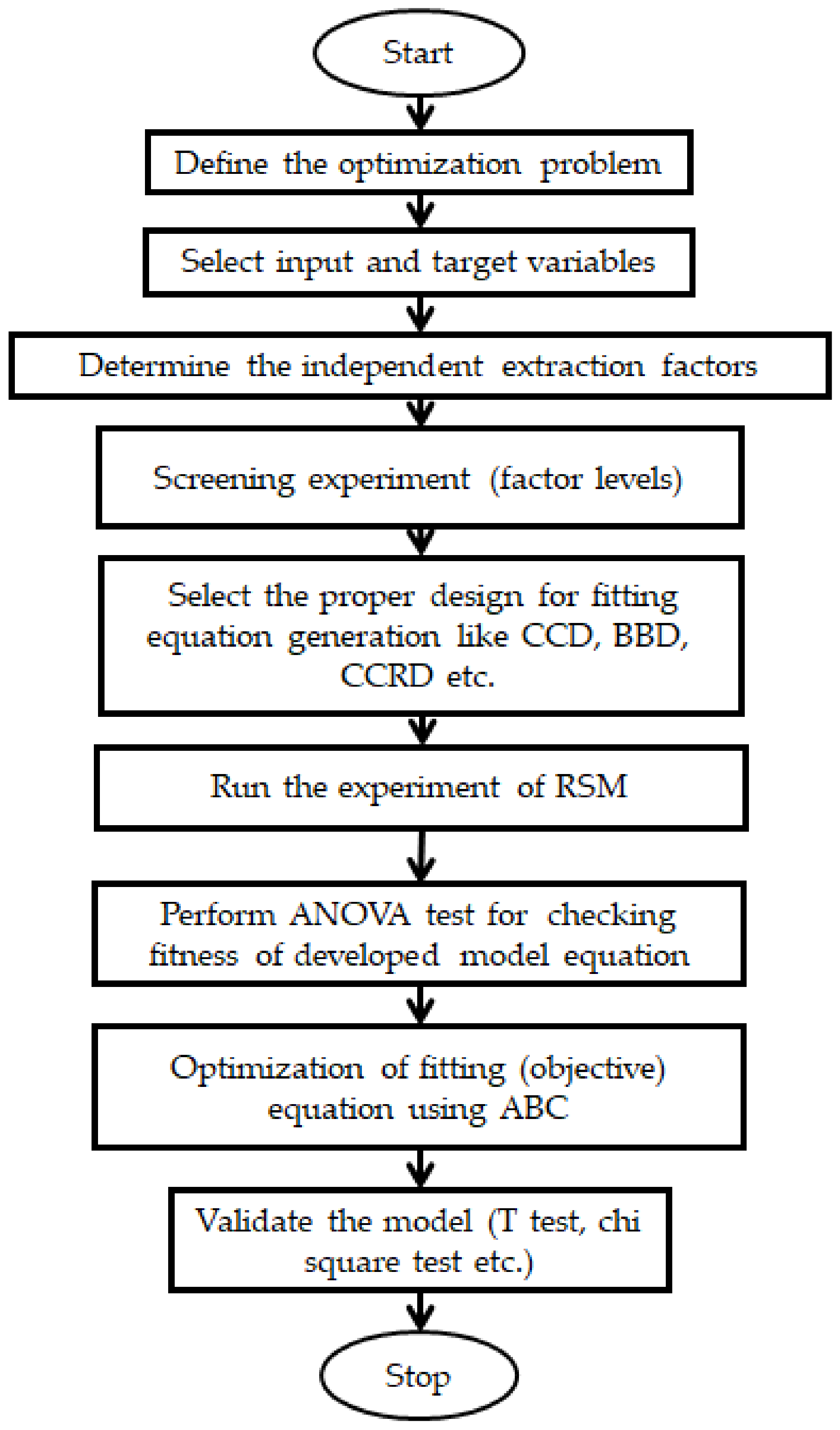
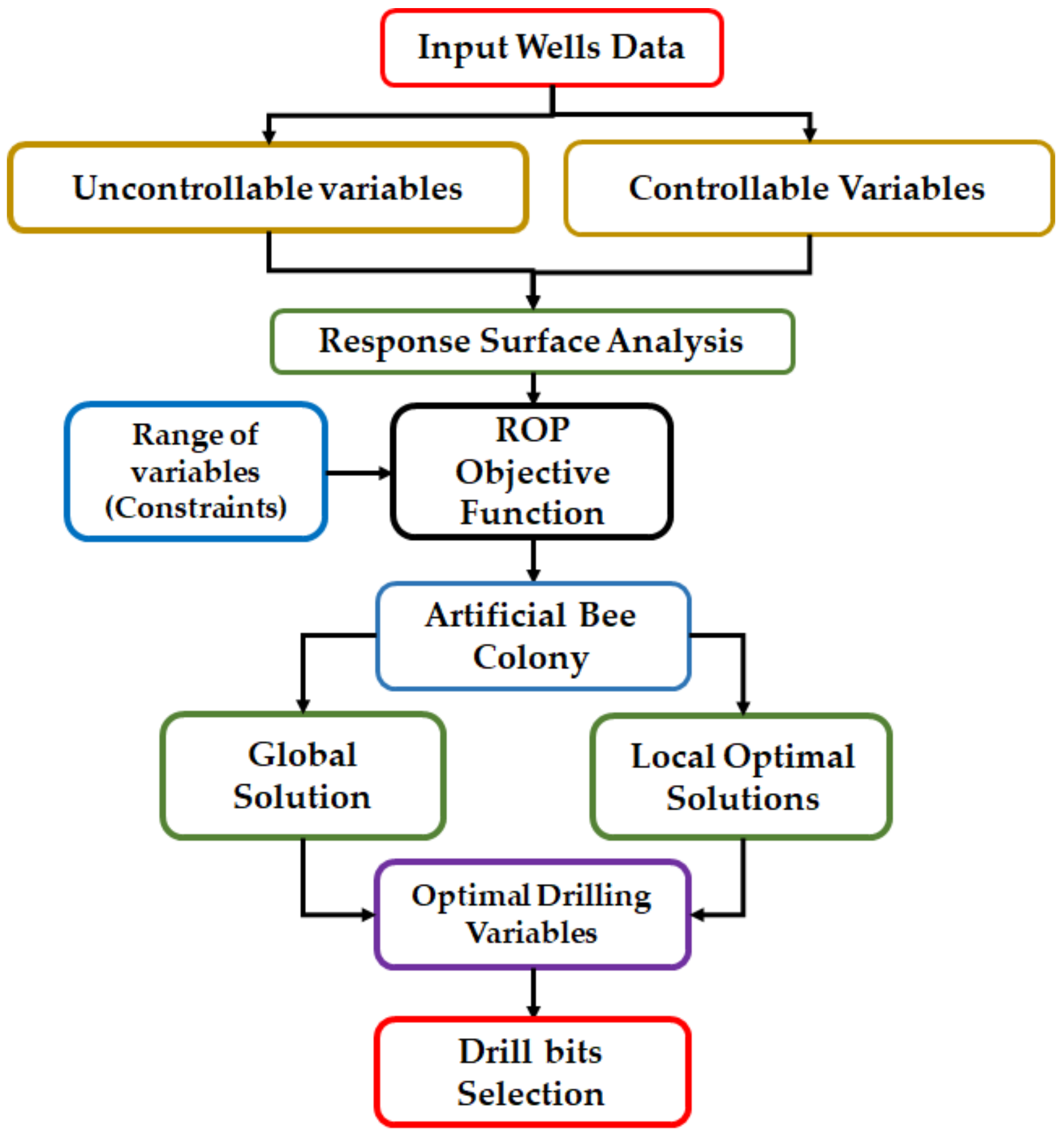
3. Materials and Methods

In this study, RSM and ABC have been utilized to develop a novel intelligent data-driven approach for the selection of suitable bit type. The performance of the existing ANN-based drill bit selection model has also been compared with the proposed approach to understand its pros and cons. This study involves the development of two separate objective functions for the same ROP and drilling variables using ANN and RSM techniques. The intelligent paradigms applied in this study are briefly explained below.

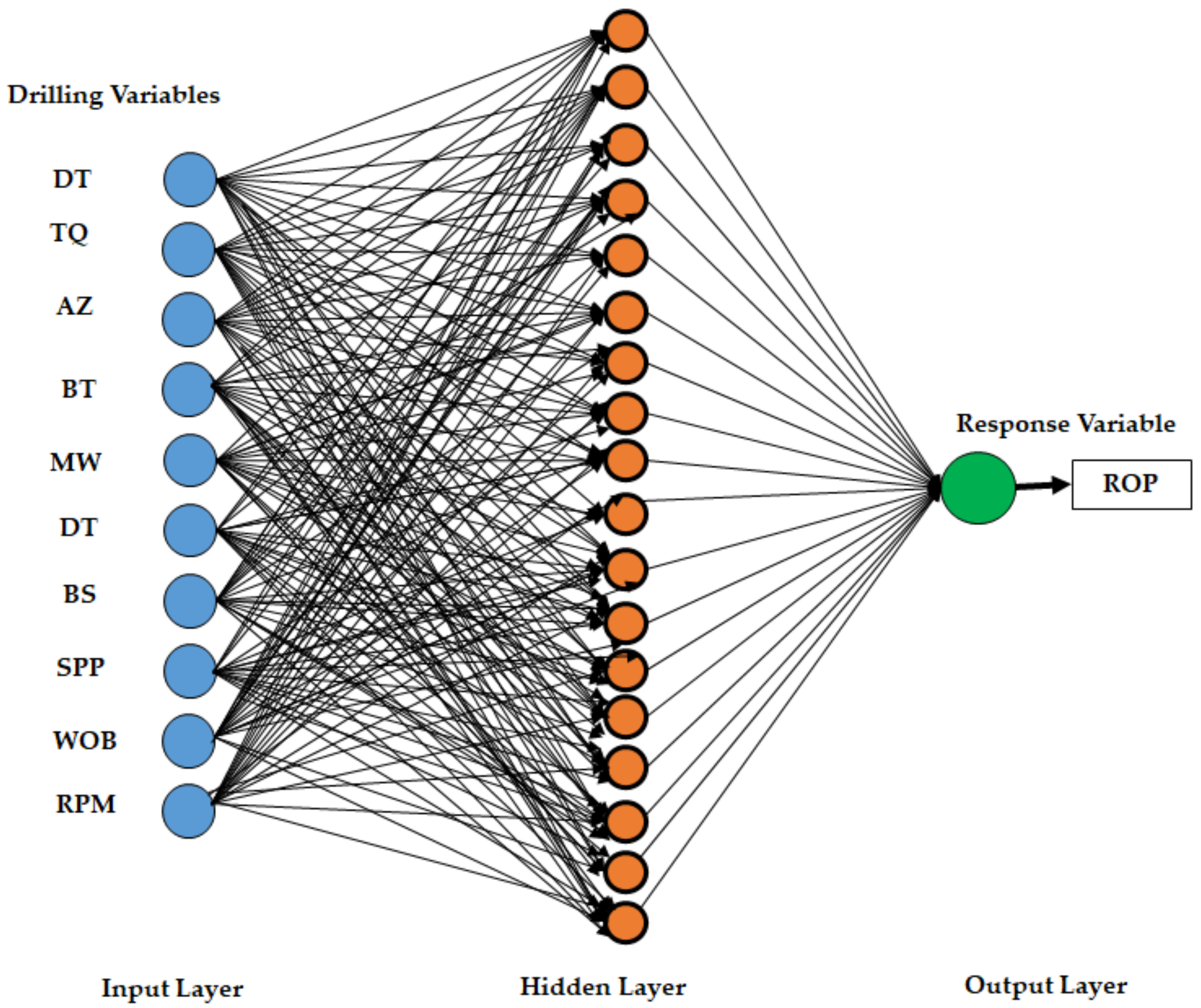
3.1. Artificial Neural Networks

ANNs are a nature-inspired intelligent paradigm that is designed based on human brain cells. It is constituted of multiple information processing units known as nodes. The interconnected nodes combine to form a layer, and layers combine to form neural networks. Neural nodes are also recognized as neuron units. Each neuron connection has been associated with weights that are attuned during the training to generate approximation function to minimize error for classification or estimation tasks. Generally, ANN comprises multilayers structure viz., input, hidden, and output layers [17]. However, the hidden layers may vary in number depending on the complexity of training data. Initially, the field data are provided to the input layer, which further transmits the raw data to hidden layers for their processing. The results acquired after processing in hidden layers are directed to the output layer, where predicted results are compared with actual target values. The deviation of prediction values from actual targets is provided as feedback to the model for updating associated weights and biases. The number of neurons and hidden layers may vary according to the complexity of problems and data types. ANN is primarily developed for handling classification and regression tasks; however, they are also applied for solving optimization problems. Figure 1 depicts the architecture of the ANN utilized in this study.

Kolmogorov’s theorem stated that multilayer feedforward perceptron (MLP) neural architecture can be utilized to define any continuous function in the form of approximation function [17,18,25]. There exist two stages in the MLP network, namely the learning stage and the prediction stage. Several neural network parameters are predetermined to define neural networks such as the number of neurons, number of layers, propagation rules, connections between neurons, activation function, learning rate, etc. The propagation rule in MLP is the weighted sum of inputs, which is given below.

$${\displaystyle \sum _{m=1}^M{w}_{mn}{x}_m(t)+{\beta }_n}$$

(3)

where w_mn is the connection weights associated with neuron m in the input layer and neuron n in the hidden layer, x_m is the outcome from neuron m in the input layer and M represents the input layer neurons, t represents the associated patterns, and ${\beta }_n$ represents neuron bias. The activation function will be multiplied with Equation (3) to decide whether neurons should be activated or not. There are several popular activation functions used in neural networks such as sigmoid function, hyperbolic tangent function, Softmax function, Softsign, Rectified linear unit, Exponential linear units, etc. The outcome from the K_th neuron with activation function existing in the input layer is given below [18].

$$Y_n=f^a({\displaystyle \sum _{m=1}^M{w}_{mn}{x}_m(t)+{\beta }_n)}$$

(4)

Due to the three-layer architecture of MLP, the propagation rule is applied twice to transmit the values from the input to the output layer. Considering N to be the number of neurons in the output layer, the result of the K_th output neuron can be described by the following equation [18].

$$Y_k=({\displaystyle \sum _{n=1}^N{w}_{nk}{Y}_m(t)+{\beta }_k)}$$

(5)

Substituting Equation (4) in Equation (5), the outcome of K_th neuron can be rewritten as given below.

$$Y_n={\displaystyle \sum _{n=1}^N{w}_{nk}\left(f^a({\displaystyle \sum _{m=1}^M{w}_{mn}{x}_m(t)+{\beta }_n)}\right)}+{\beta }_k$$

(6)

Equation (6) of MLP is utilized to approximate the objective function in optimization as given in Equation (7) [18].

$$f(x_1,x_2\dots x_M)={\displaystyle \sum _{n=1}^N{w}_{nk}\left(f^a({\displaystyle \sum _{m=1}^M{w}_{mn}{x}_m(t)+{\beta }_n)}\right)}+{\beta }_k$$

(7)

Constraints

$$\begin{gathered} C_1(x_1,x_2\dots x_M)\le 0 \\ {C}_n(x_1,x_2\dots x_M)\le 0 \end{gathered}$$

Equation (7) acts as the objective function and constraints for optimization problems where the relationship between input and response variable is undefined. In the case of complex approximation function, algorithms such as Ant Colony, Particle Swarm Optimization, ABC, GA, etc., can be applied to retort the optimization problem.

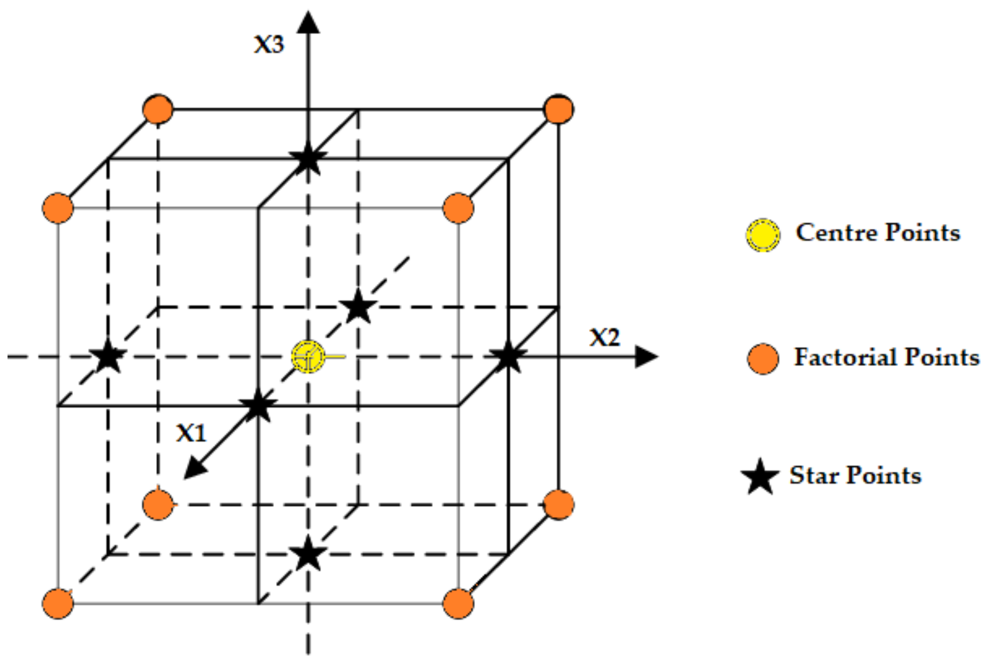
3.2. Response Surface Methodology

RSM is a set of statistical techniques that are quite helpful in optimizing, developing, and improving processes and useful in analyzing and modeling numerous problems in engineering [26,27]. RSM is particularly useful in real-world situations where various variables affect the performance, quality, and output of the desired process as in the case of drilling operations [27]. The target variable (Y) is termed as the response variable, while input variables are known as independent variables. An appropriate relationship can be identified between input and response variables using RSM. RSM helps to develop the correct approximate mathematical function, which satisfies a suitable relationship between the objective function and test factor group [26]. Interaction between the input variables can also be included in the response surface equation. The generalized relationship can be developed as given below.

$$y=f(X_n)+e\sqrt{2}$$

(8)

where f is the unknown exact response function, which may be complex, and e is the error due to unaccountable factors that influence the response or output but are never included in the Equation (8) such as noise, interaction effects, etc. Let us consider that e is a statistical error that is distributed normally with variance ${\sigma }^2$ and zero mean. Then, the following error equation can be written as given below.

$$Error[Y]=Error[f(X_n)]+Error[e]=f(x_1,x_2\dots x_n)$$

(9)

where $x_1,x_2,\dots x_n$ are known as natural variables in their natural units. Furthermore, these variables are changed into coded variables that are dimensionless and have zero mean and alike standard deviation. The coded form of Equation (9) is written as given below.

$$\mu =f(x_1,x_2\dots x_n)$$

(10)

Here, function f is known and undefined. Thus, a suitable approximation function is required to be generated for modeling purposes. In RSM, the first or second-order polynomial equation is primarily generated as approximation functions in place of the actual response function. The second-order model is popularly applied for modeling various process operations due to its flexibility, diverse functional form, efficient approximation, and model coefficients that can be easily estimated through the least square estimation technique. A second-order response surface equation, based on Talyor series expansion, is given below:

$$y_T={\beta }_0+i={\displaystyle \sum _{i=1}^n{\beta }_i}{x}_i+{\displaystyle \sum _{i=1}^n{\beta }_{ii}{x}_i^2}+{\displaystyle \sum {\displaystyle \sum _{i<j=2}^n{\beta }_{ij}}{x}_i{x}_j+\epsilon }$$

(11)

where x_i and x_j represent the input parameters, b₀ is the constant of the regression equation, Y is the predicted ROP response, ${\beta }_i$ is the linear coefficients, ${\beta }_{ij}$ are interaction coefficients, ${\beta }_{ii}$ are the coefficients of the square terms, and $\epsilon$ is the fitting error in the equation. To generate a response surface, stepwise regression methods are utilized to reduce the computational burden.

Here, central composite design (CCD) has been considered for developing the second-order approximation function for ROP, as shown in Equation (11). The input variables are converted into coded variables for fitting the data in CCD between two levels [−1, 1]. CCD contains the factorial point, central point, and axial points, which are mostly developed through sequential experimentation, as shown in Figure 2. Ten factors and full factorial design were utilized for the development of the response function. The range of design factors was assigned according to the range of field variables. The interaction, quadratic, and linear coefficients were estimated through the least square regression. Furthermore, the importance of each term was determined through an analysis of variance (ANOVA) test, whereas redundant terms were eliminated. Equation (11) will act as an ROP objective function (approximation function) for the target geological formations containing bit information as an input variable similar to ANN. Furthermore, this equation will be optimized using Artificial Bee Colony to find the optimum value of ROP along with its input variables (control variables) including BT. A comprehensive explanation of RSM is available in the cited literature [26,27]. Figure 3 provides a flowchart of RSM for the development and optimization of the ROP equation.

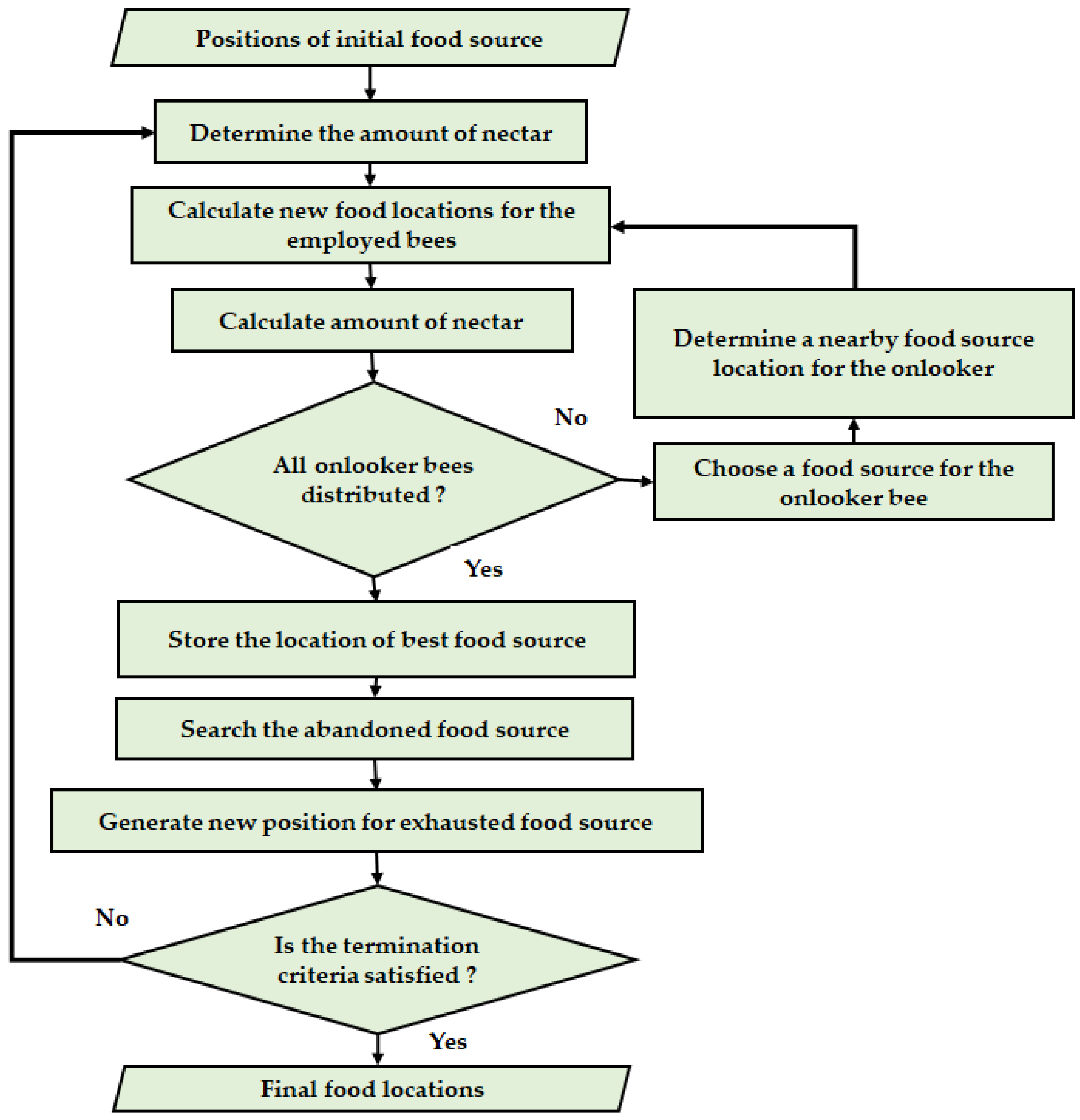
3.3. Artificial Bee Colony

Karaboga (2005) proposed an Artificial Bee Colony (ABC) paradigm based on the natural behavior of bees when they search for nectar containing flowers [28]. There are three variations of honey bees generally present in natural hives, namely onlookers, employed bees, and scouts. Every bee has an assigned duty that it is required to perform. The scout bees perform a random hunt for the flowers that have nectar in their nearby environment and remember the location of the flower inside their internal memory [28]. This means scouts examine local search feature space for optimal solutions and remember it. After returning to their hive, scouts exchange information about flower location with other bees using the waggle dance technique [28]. After the waggle dance, employed bees begin their exploration for the nectar-having flowers depending upon the information achieved from scout bees. The employed bees extract the nectar from the target flowers, which are known as food sources [28]. Only one employed bee will be assigned to a single flower to exploit their nectar. Thus, each available food source contains an assigned employed bee that creates an initial solution [28]. The value of each solution is calculated to understand its significance. A new response is generated for each problem solution using the relationship as given below.

$$B_{i,j}=S_{i,j}+{\delta }_{i,j}(S_{i,j}-S_{k,j})$$

$$i\in \left\{1,2,\dots IA\right\},j\in \left\{1,2,\dots O\right\},k\in \left\{1,2,\dots IA\right\}andk\ne i$$

(12)

where $S_{i,j}$ is parameter j obtained from response i, $B_{i,j}$ is the parameter j in the new response, whereas i represents the number of solutions, ${\delta }_{i,j}$ is an arbitrary number existing between [−1, 1], k is a random number from a single answer to the problem, IA signifies initial solutions to the given problem, and O is the total number of parameters required during optimization. After calculating a new answer for each solution, they are compared with the previous answer. If the difference is found to be higher between the current and earlier answer, only then it will be accepted; otherwise, it will be rejected [28]. The step length is adaptively decreased according to the difference between current and previous answers as the search reaches closer to the optimal solution. The waiting onlooker bees in the hive choose the best source depending upon the dance of employed bees. This helps in identifying the global solution existing in the search space along with local solutions [28]. Furthermore, employed bees of an abandoned food site start to behave like scout bees and hunt for newer sources of food. The probability of selection of source through an onlooker bee is given below.

$$\mathrm{Pr}{o}_i=\frac{fitness}{{\displaystyle {\sum }_{n=1}^{FS}fitnes{s}_n}}$$

(13)

where $fitnes{s}_i$ represents the fitness of the solution i examined via employed bees depending upon nectar quantity at location i, and FS is the number of the food source. After predefined iterations, there is no improvement in answer value using Equation (12); then, the employed bees convert into scouts and randomly begin the search for a newer source of food. The ABC algorithm has been utilized for solving various engineering problems such as ROP optimization [29], oil and gas well placement optimization [30], over break prediction in the tunnel [31], etc. A detailed description of ABC optimization can be found in other references [31,32,33,34]. Figure 4 depicts the flowchart of the Artificial Bee Colony paradigm that was originally proposed by Karaboga [28]. Figure 5 shows the generalized schema of the proposed approach of drill bit selection.

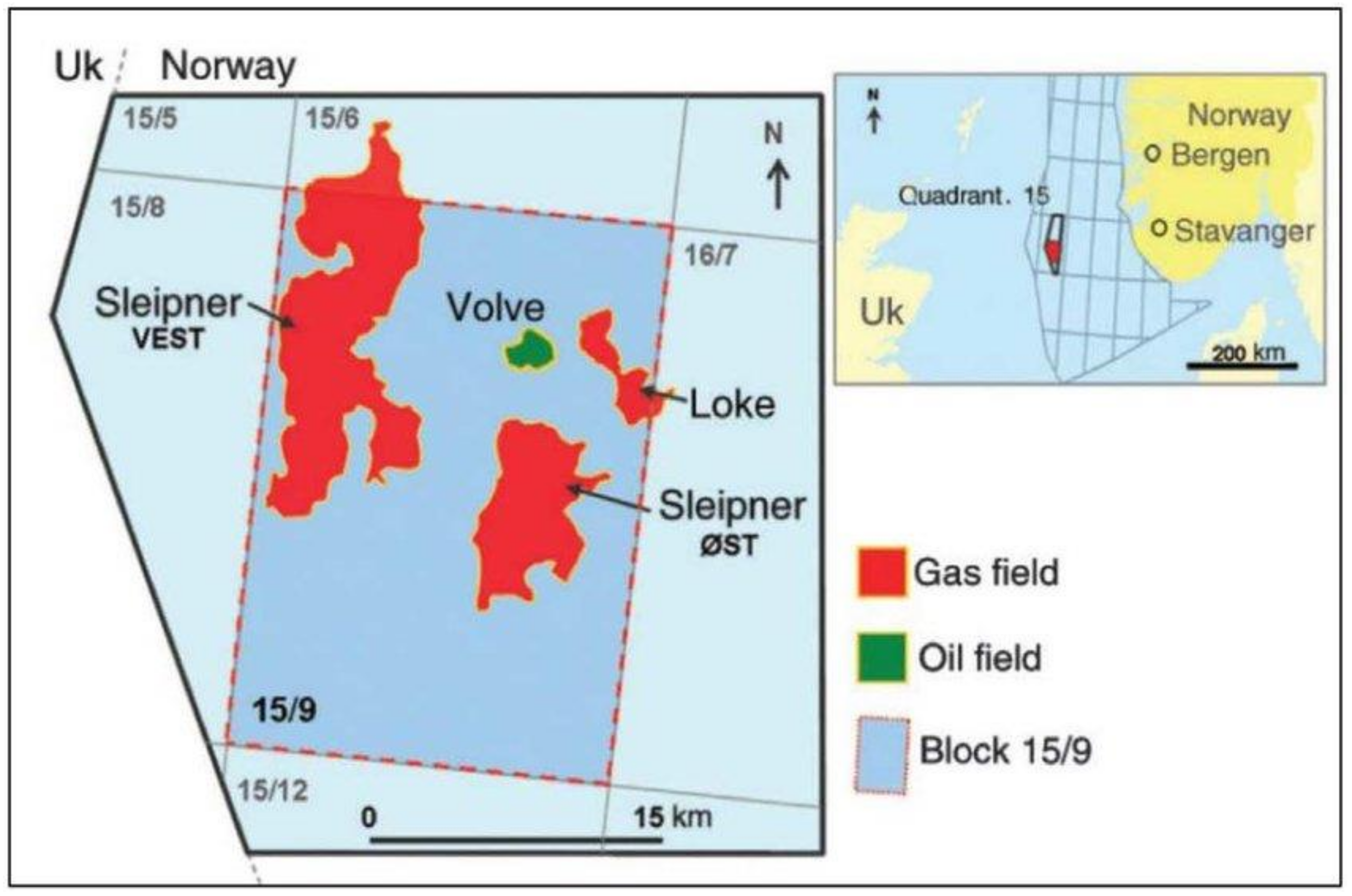
3.4. Data Description

The Volve oil and gas field is situated in the central North Sea near the Norwegian Continental Shelf. It was discovered in 1993 and its production shut down in September 2016 by its investors’ companies. The ocean depth near the Volve field is in a range of 85 to 95 meters. This field contains Jurassic sandstone related to the Hugin formation reservoir. The depositional environment of this reservoir is analyzed as tidal to the shallow estuary. The average properties expected from this Hugin reservoir are as follows: porosity (0.2), permeability (910), water saturation (0.23), and shale volume (0.17). Geosteering was particularly utilized to increase the extent of the reservoir linking to various fault blocks. The peak production rate in the Volve field was recorded to be 56,000 barrels per day and produced a cumulative amount of 63 million barrels of oil with a recovery rate of 54% of the total reservoir estimated over 8 years [35]. Input data used in this research work were obtained from the Equinor company website openly available for research purposes [35].

Table 1. Geological prognosis of Well 15/9-F-12 under study (courtesy: Equinor company) [35] *.

Group	Formation	Depth (m)	Description
Nordland	Utsira Top	892	Gray claystone, a stringer of sand and siltstone.
	Utsira Base	1084	Well-sorted sandstone, minor silt, and limestone stringers.
Hordaland	Skade Top	1259	Claystone, minor limestone/dolomite stringers.
	Skade Base	1347	Medium-grained sorted sandstone.
	Grid Top	2179	Fine-grained sandstone.
	Grid Base	2245	Fine-grained sandstone.
Rogaland	Balder Top	2317	Colored claystone, partly tuffaceous, and limestone stringers.
	Sele Top	2374	Claystone and limestone stringer.
	Lista Top	2445	Non-calcareous claystone and minor limestone stringers.
	Ty Top	2531	Fine to medium sandstone; some interbedded claystone, siltstone, and limestone stringers.
Shetland	Ekofisk Top	2698	Limestone with traces of claystone and sandstone.
	Tor Top	2715	White limestone with traces of claystone.
	Hod Top	2839	Limestone along with gluconate.
	Blodoeks Top	2944	Marl, argillaceous laminations, and gluconates in parts.
	Hidra Top	2972	Off-white firm limestone.
Cromer Knoll	Roedby Top	2981	Marl along with argillaceous laminations
	Aasgard Top	3001	Interbedded limestone and marl with minor claystone and siltstone.
Viking	Draupne Top	3036	Organic-rich claystone, micaceous, carbonaceous with traces of pyrite.
	Heather Top	3086	Claystone with limestone stringers.
Vestland	Hugin Top	3094	Sandstone and rare claystone stringers.
	Sleipner Top	3266	Sandstone, grey claystone, and layers of coal.

* Table showing different formations existing for F-12 well along with the depth of the reservoir.

contains the geological prognosis of the Volve field.

Table 2. Statistical details of drilling data used in this study.

S. No.	Drilling Variables	Ranges	Units	Code Factor
1.	Measured Depth (DT)	100–3520	m	$x_1$
2.	Rate of Penetration (ROP)	1.73–201.02	m/h	--
3.	Weight on bit (WOB)	0.01–19.17	Tons	$x_2$
4.	Rounds per minutes (RPM)	60–220	rpm	$x_4$
5.	Torque (TQ)	0–5.24	kN/m	$x_3$
6.	Standpipe pressure (SPP)	58.6–289.2	Bar	$x_5$
7.	Mud weight (MW)	1.03–1.42	S.g.	$x_6$
8.	Inclination (IN)	0.46–54.95	Degree	$x_8$
9.	Azimuth (AZ)	0.38–334.67	Degree	$x_9$
10.	Bit type (BT)	1–11	N/A	$x_{10}$
11.	Bit Size (BS)	8.5–26	Inch	$x_7$

contains a description of the drilling variables used in the study.

Table 3. Drill bit types utilized for drilling of wells at different depths for three Norwegian Volve field wells.

Well Name	Bit Type	Depth In (m)	Depth Out (m)	IADC Code	Bit Size (Inch)
WELL A (F-4)	1	100	310	PDC M415	36″
	2	25	1360	MT 115A	17.5″
	7	1360	1410	PDC M422	12.25″
	8	2770	2993	PDC M222	8.5″
	8	2993	3510	PDC M222	8.5″
Well B (F-15)	10	144	226	MT 115	36″
	6	226	1378	PDC M115	26″
	3	1378	1381	MT 244	17.5″
	4	1381	2536	PDC M332	12.25″
	9	2536	3670	PDC M323	8.5″
	9	3670	4090	PDC M323	8.5″
	5	1378	2591	PDC M322	26″
	4	2591	2594	PDC M332	12.25″
	5	2591	2596	PDC M322	8.5″
	5	2596	3180	PDC M322	8.5″
	5	3180	4095	PDC M322	8.5″
	5	3185	3498	PDC M322	8.5″
	7	2562	2665	PDC M422	12.25″
	7	2665	2920	PDC M422	12.25″
WELL C (F-12)	1	251	1369	PDC M415	36″
	5	1369	2513	PDC M322	17.5″
	6	2513	2573	MT 135	17.5″
	7	2573	3114	PDC M422	12.25″
	8	3114	3520	PDC M222	8.5″

has been provided to inform about different drill bit types (IADC code) utilized for drilling the three wells. Wells A (F-4) and B (F-15) were utilized for the training of models and well C (F-12) was used for testing the developed models. The IADC code of drill bits cannot be utilized directly for the training of the ANN model. Thus, they are numbered in the bit-type column of Table 3. The location of the Norwegian Volve field situated in the North Sea is depicted in Figure 6.

4. Results

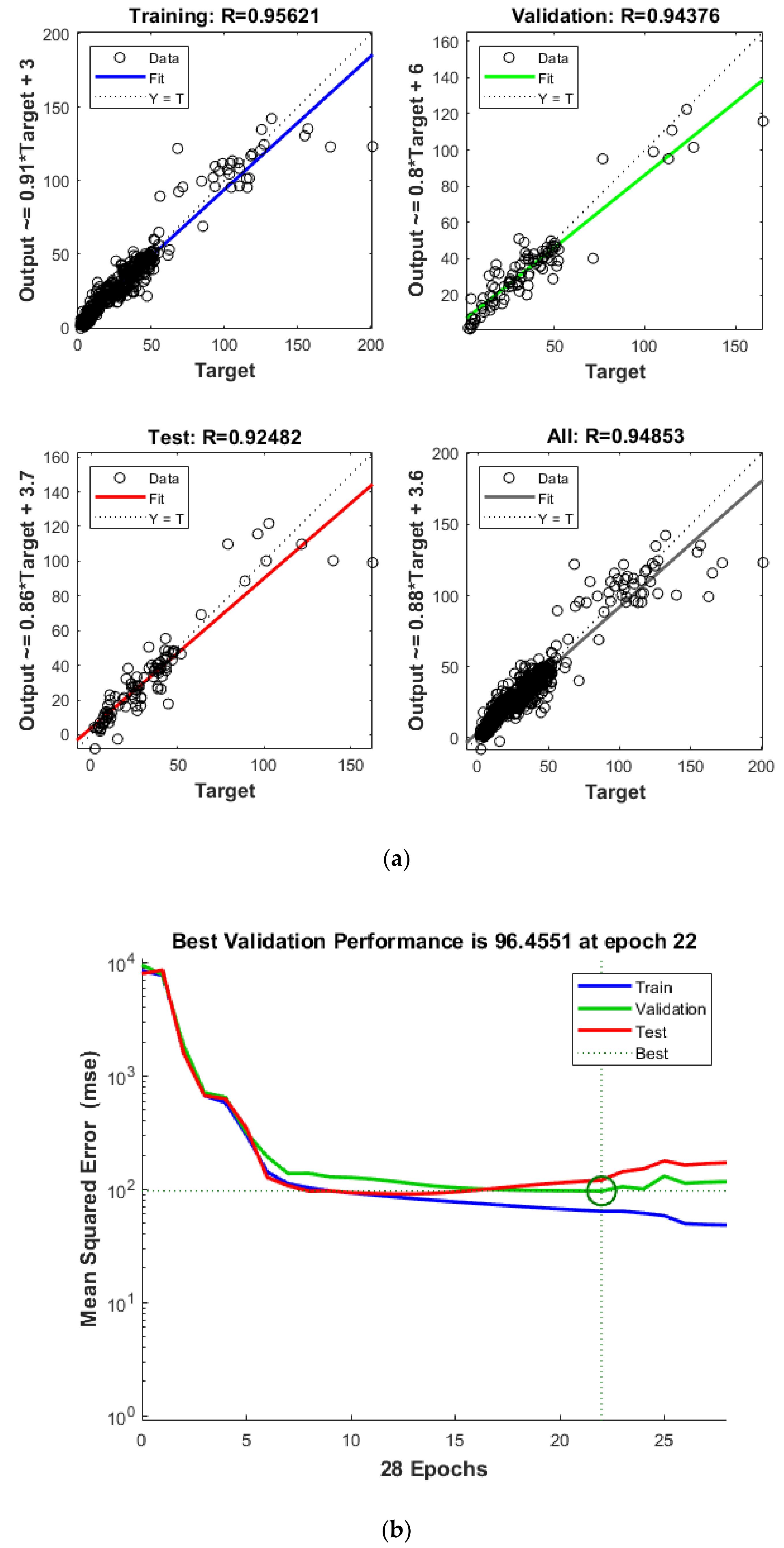
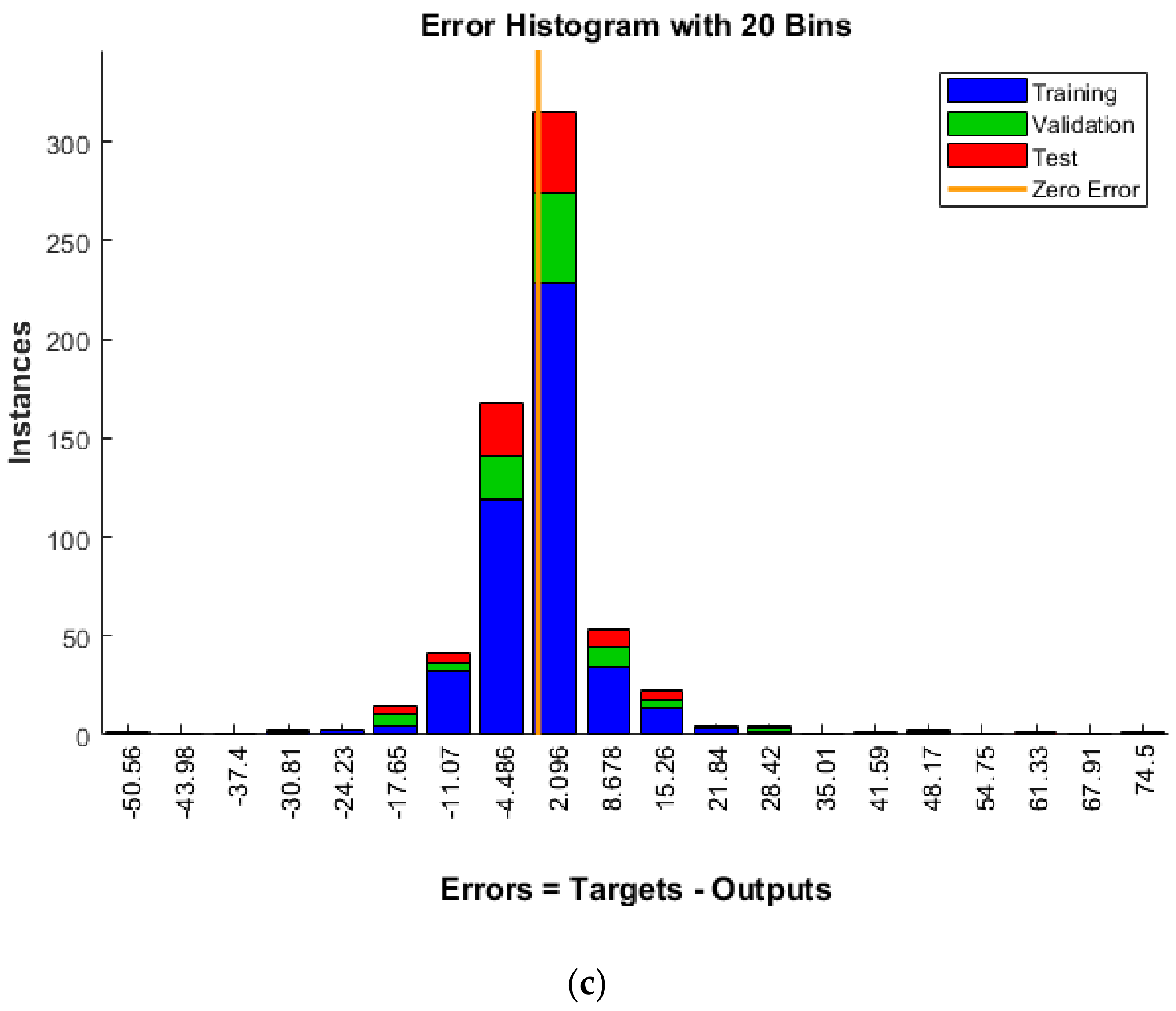
4.1. Development of ROP Objective Function Using ANN

In this study, three-layered MLP architecture was utilized to generate an approximation function for the ROP in terms of operational drilling variables. ANN having a three-layered multilayer perceptron architecture can be utilized to produce the polynomial equation for solving optimization problems [18]. However, parameters of ANN are required to be determined beforehand during the training stage. Three popular training functions were applied to train the ANN, namely (a) Levenberg–Marquardt (LM), (b) Scaled Conjugate Gradient (SCG), and (c) Bayesian Regularization (BR). Hornik et al. [36] suggested that a singular hidden layer neural network model can be utilized for approximating any nonlinear function. Still, the optimum neurons in the hidden layer are required to be estimated before training the ANN model.

Table 4. The reported relationships to calculate the neurons inside the hidden layer of ANNs.

Relationships	References
$\le 2\times N_i+1\prime$	[25]
$\left(N_i+N_0\right)/2$	[37]
$\frac{2+N_0\times N_i+0.5N_0\times (N_0^2+N_i)-3}{N_i+N_0}$	[38]
$2\times N_i/3$	[39]
$\sqrt{N_i\times N_0}$	[40]
$2N_i$	[41,42]

contains reported correlations to decide the number of neurons inside the hidden layer. N_i and N_o represent the number of predictor and target variables in Table 4. Several ANN models were generated with the neurons ranging from 2 to 20 which, were calculated using the correlations available in Table 4. The optimum values of the model parameters are given in

Table 5. Optimum values of model parameters utilized in this research work.

Estimators	Model Parameters	Search Range	Optimum Value
ANNs	Configuration	2–20	[10-18-1]
	Learning rate	0.0001–0.5	0.0001
	Maximum number of iteration	100–1000	200
	Activation function hidden layer	Tangential sigmoid function	N/A
	Activation function output layer	purline function
	Training algorithm	Levenberg–Marquardt	N/A
ABC	Iterations	10–200	100
	Scouts	1–100	70
	Colony size	1–100	100
GA	Iterations	1–5000	3000
	Crossover probability	0.1–1	0.5
	Population size	1–200	100
	Crossover type	-	Uniform
	Elit_ratio	0.001–1	0.001
	Parents portion	0.1–1	0.3

.

The performance of developed ANN models are compared based on the coefficient of correlation (R²) and root mean square error (RMSE) as mentioned below.

A. Coefficient of correlation (R²):

$$R^2=\frac{{\displaystyle \sum _{i=1}^n{(RO{P}_m-RO{P}_p)}^2}}{{\displaystyle \sum _{i=1}^n{\left[RO{P}_m-\frac{1}{n}{\displaystyle \sum _{i=1}^n(RO{P}_m)}\right]}_i^2}}$$

(14)

B. Root mean square error (RMSE):

$$RMSE=\sqrt{\frac{1}{n}{\displaystyle \sum _{i=1}^n{(RO{P}_m-RO{P}_p)}^2}}$$

(15)

Zorlu et al. [43] suggested a ranking method to compare the performance of several neural networks together. Here, an integer (rank) was allocated to every network based upon the goodness of R² and RMSE values. Then, ranks allocated to every R² and RMSE were added to acquire the total rank for every network configuration separately. The network having the highest total rank was considered as the best model for this research work [44]. The results of three-layered neural architectures with three different combinations of training functions are recorded in

Table 6. The outcomes of ANN models trained using the Levenberg–Marquardt (LM) function *.

Model No.	No of Neurons	Train R2	Train RMSE	Test R2	Test RMSE	Train Rating R2	Train Rating RMSE	Test Rating R2	Test Rating RMSE	Total Rank
1	2	0.793	11.76	0.597	20.414	3	3	1	1	8
2	4	0.640	16.20	0.634	16.233	1	1	2	2	6
3	6	0.839	10.94	0.720	14.975	4	5	3	4	16
4	8	0.894	9.283	0.850	8.298	6	6	9	10	31
5	10	0.843	11.18	0.801	10.475	5	4	6	8	23
6	12	0.930	6.930	0.831	13.635	9	8	8	5	30
7	14	0.908	8.332	0.761	11.786	8	7	4	7	26
8	16	0.952	6.319	0.825	16.392	10	9	7	3	29
9	18	0.9143	7.99	0.855	10.32	7	10	10	9	36
10	20	0.734	14.59	0.774	12.916	2	2	5	6	15

* Table 6 shows the ranking method for selecting the optimum number of neurons for the hidden layer. Here, 18 neurons have achieved the highest total rank of 36 by summing all the training and testing ratings together for the LM training function. The results are also compared with the total rank achieved in Table 7 and Table 8 to decide the optimum neuron configuration in the hidden layer.

,

Table 7. The outcomes of the ANN models trained using the Scaled Conjugate Gradient (SCG) function.

Model No.	No of Neurons	Train R2	Train RMSE	Test R2	Test RMSE	Train Rating R2	Train Rating RMSE	Test Rating R2	Test Rating RMSE	Total Rank
1	2	0.723	14.82	0.675	16.430	4	4	4	4	16
2	4	0.767	12.71	0.804	12.901	8	8	2	9	27
3	6	0.558	19.32	0.648	16.520	1	2	2	3	8
4	8	0.710	14.30	0.673	14.263	3	6	3	7	19
5	10	0.685	16.34	0.600	14.340	2	3	1	6	12
6	12	0.764	13.88	0.816	11.778	7	7	9	10	33
7	14	0.814	12.37	0.756	13.538	10	9	7	8	34
8	16	0.734	14.36	0.745	14.609	5	5	6	5	21
9	18	0.802	12.12	0.733	16.851	9	10	5	2	26
10	20	0.757	210.75	0.869	115.82	6	1	10	1	18

and

Table 8. The outcomes of the ANN models trained using the Bayesian Regularization (BR) function.

Model No.	No of Neurons	Train R2	Train RMSE	Test R2	Test RMSE	Train Rating R2	Train Rating RMSE	Test Rating R2	Test Rating RMSE	Total Rank
1	2	0.855	10.84	0.714	13.376	1	1	3	8	13
2	4	0.890	8.90	0.819	13.520	2	3	7	6	18
3	6	0.927	7.58	0.751	13.375	3	4	5	9	21
4	8	0.9281	6.94	0.864	13.473	4	5	9	7	25
5	10	0.946	6.492	0.762	14.476	6	6	6	4	22
6	12	0.946	6.359	0.907	10.059	6	7	10	10	33
7	14	0.965	5.131	0.547	19.724	8	9	1	2	20
8	16	0.960	5.37	0.820	14.157	7	8	8	5	28
9	18	0.973	4.416	0.715	19.234	9	10	4	3	26
10	20	0.986	9.907	0.562	28.045	10	2	2	1	15

. The training algorithm LM has acquired the highest rank of 36 through its performance with (10-18-1) configuration. Therefore, the best performing ANN (10-18-1) alignment was considered for the development of the approximation function to obtain optimum values ROP and Bit Type (BT) along with other drilling variables. All the ANN variants are developed using MATLAB 2019 software.

Figure 7 contains the Regression plot, Mean square error (MSE) plot, and Error plot of optimal ANN architecture [10-18-1].

Table 9. The weights and bias allocated to the training of optimal ANN configuration [10-18-1].

Connections	Generated Values
Bias Hidden Layer	−2.331; −2.775; −0.1308; −0.03132; 1.504; 0.2345; 2.2617; −1.5475; 1.1458; 0.3785; −0.0855; 0.3141; −1.0727; −2.2302; 1.8623; −2.6596; −1.85; 2.721
Connection Weights between Input and Hidden Layer	−0.486; −2.186; 0.151; 1.236; 1.964; 0.920; −0.5052; −0.677; 0.008; 0.570; 1.202; −0.577; 0.269; −2.421; 0.145; −0.654; −0.664; −2.189; 1.061; 0.126; 1.048; 1.962; −0.479; −0.984; −1.578; 0.542; −1.061; −0.900; −0.856; 0.401; 0.108; −0.469; −1.358; −0.818; 0.037; 0.413; 0.484; −1.092; −1.283; 0.109; −0.444; −1.698; −3.35; 0.353; −0.194; −0.038; −0.431; −0.647; −0.0049; −0.225; 0.266; 0.517; −0.0142; 1.035; 0.456; −0.271; 0.6465; −0.568; 1.96; −0.423;−0.594; −0.981; 0.441; −0.363; −0.293; −0.0681; −0.313; −0.996; −2.33; 1.21; −1.033; −0.649; 1.68; −0.859; 0.426; 0.880; −0.425; −1.456; −1.231; 0.436; −1.234; −1.301; 1.712; 1.96; 1.55; 0.53; 1.17; −1.79; 0.66; −0.093; −2.81; 1.47; −1.103; −0.346; −3.252; 0.403; −0.52; 0.426; −1.246; 0.8551; −0.721; −3.845; 0.619; 0.902; 1.909; −0.7886; 0.271; 1.015; −3.98; 0.366; −0.101; −1.257; 2.83; 1.017; 1.185; −0.150; −0.0382; −2.389; −0.740; −1.086; −1.868; −0.573; −0.689; −0.337; −1.414; 1.336; 0.797; −0.853; −2.783; −0.484; −0.252; −1.243; 1.548; 1.508; 0.047; −0.109; 0.699; 0.56544; −0.317; −0.452; 1.35; −0.1153; −0.661; 1.076; 0.436; 0.986; 0.55; 0.5131; −1.026; −0.5348; −0.1402; 0.156; −0.5217; −0.6648; 1.3074; 0.0939; −0.822; −1.814; −0.092; 1.22; 0.242; −1.53; 1.24; −1.493; 0.112; −0.68; −0.342; 0.62; 0.451; −0.179; −1.14; 3.38; 0.66; −0.351; −0.017; 0.098; −0.433; −1.99; −1.40; −0.112
Bias Output Layer	−0.7816
Connection Weights between Hidden Layer and Output Layer	−0.264; −1.214; 0.0348; −0.701; 0.319; 0.410; 0.1114; 0.421; 0.5133; −0.4028; 0.1325; −0.5300; 0.785; −0.475; −0.765; 0.434; 0.376; −0.133

contains weights and bias associated with the selected neural network configuration (10-18-1). The developed ROP approximation function using Equation (7) is given below.

$$f(x)=\left[{\displaystyle \sum _{i=1}^N{w}_{2,1}}\left(\frac{1}{\left[1+e^{-2z}\right]}-1\right)+b_2\right]$$

(16)

$$z=(w_{i,1}\times x_1+w_{i,2}\times x_2+w_{1,3}\times x_3+w_{i,4}\times x_4+w_{i,5}\times x_5+w_{i,6}\times x_6+w_{i,7}\times x_7+w_{i,8}\times x_8+w_{i,9}\times x_9+w_{i,10}\times x_{10})$$

where the tangent sigmoid function is utilized in the hidden layer, and purline is the activation function for the output layer. w_i,1 and w_2,i are the weights of input and hidden layers. The weights and bias (obtained during the training of 10-18-1 ANN configuration) associated with the Equation (16) have been provided in Table 9.

Table 10. Range of predictor variables utilized during the optimization of ROP as upper and lower bounds.

Depth Interval (m)	Predictor Variables Utilized During Optimization
251–1369	DT = constant, BT = [1, 10], BS = constant, WOB = [0.01, 16.29], RPM = [83, 220], TQ = [−0.15, 15.26]. MW = [1.03, 1.36], IN = constant, AZ = constant, SPP = [59, 153]
1369–2513	DT = constant, BT = [1, 10], BS = constant, WOB = [0.01, 19.17], RPM = [90, 186], TQ = [7.58, 27.03]. MW = [1.16, 1.4], IN = constant, AZ = constant, SPP = [140, 252]
2513–2573	DT = constant, BS = constant, BT = [1, 10], WOB = [11.78, 19.07], RPM = [150, 180], TQ = [11.35, 19.07]. MW = [1.39, 1.4], IN = constant, AZ = constant, SPP = [226, 282.4]
2573–3114	DT = constant, BT = [1, 10], BS = constant, WOB = [1.35, 10.96], RPM = [137, 180], TQ = [1.07, 9.84]. MW = [1.39, 1.42], IN = constant, AZ = constant, SPP = [220, 290]
3114–3520	DT = constant, BS = constant, BT = [1, 10], WOB = [2.04, 6.87], RPM = [60, 140], TQ = [2.11, 6.15]. MW = [1.39, 1.44], IN = constant, AZ = constant, SPP = [174.6, 233.9]

contains constraint bounds required for the optimization of the ROP Equation (16) and control variables. Here, measured depth (DT), Inclination (IN), and Azimuth (AZ) will remain constant because of their predefined nature while optimizing for a particular depth.

Drill bit selection based on optimum ROP values is a bound constrained maximization problem. The developed ROP objective function (Equation (16)) requires an optimization algorithm for determining optimum values of ROP and other operational variables along with BT. GA is an evolutionary paradigm that has been utilized for the optimization of Equation (16) [44]. During the optimization process, Equation (16) was maximized using GA with upper and lower bounds as shown in Table 10 according to the following steps:

(a)

Adjust the model parameters of GA (maximum no of iterations = 3000, crossover probability = 0.5, population size = 100, parents portion = 0.3, crossover-type = uniform, elite ratio = 0.01, variable type = real);

(b)

Set the upper and lower bounds for input variables existing in objective Equation (16) using Table 10;

(c)

Randomly generate the initial population for GA;

(d)

Several combinations of ROP and input variables will be generated during optimization. In the end, GA converges on the best combination of input variables having maximum ROP value;

(e)

Record the value of ROP and BT in the final solution produced by GA. GA will provide optimum ROP values along with suitable BT and other control variables.

The optimization of the ROP objective function (Equation (16)) has been carried out using Python package Geneticalgorithm 1.0.1 freely available online for research purposes.

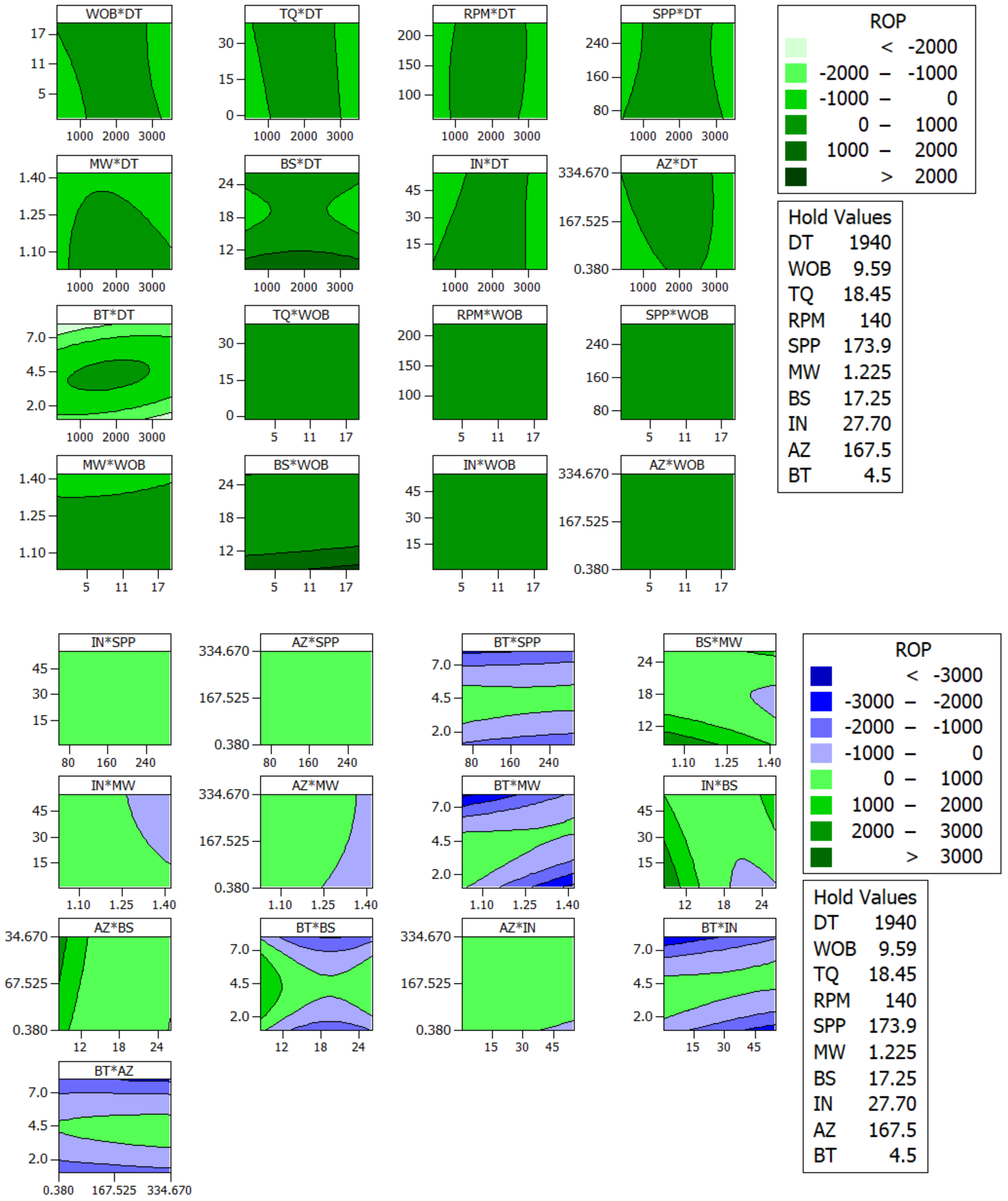
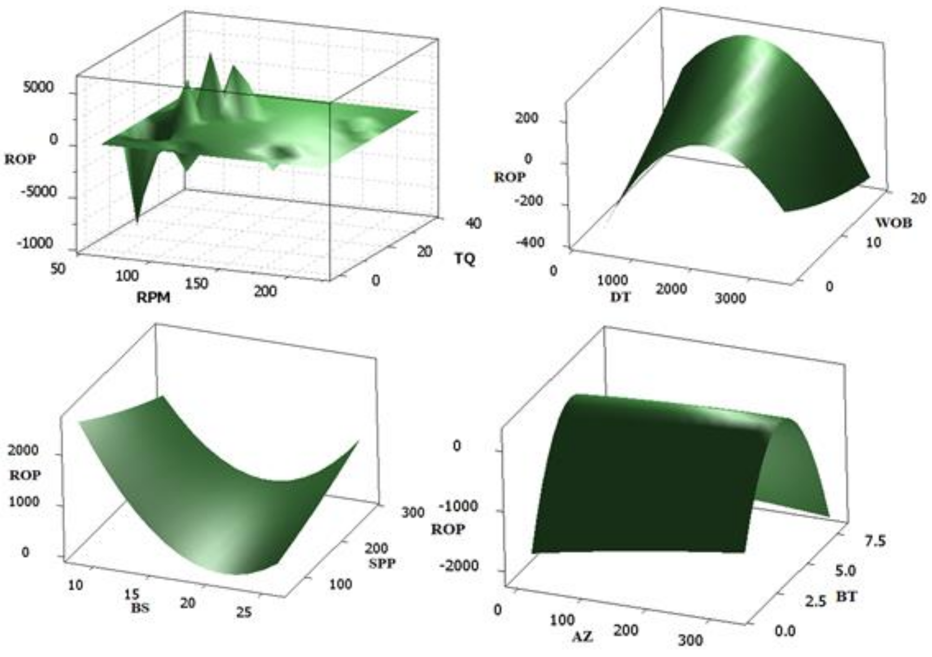
4.2. Development of the ROP Function Using RSM

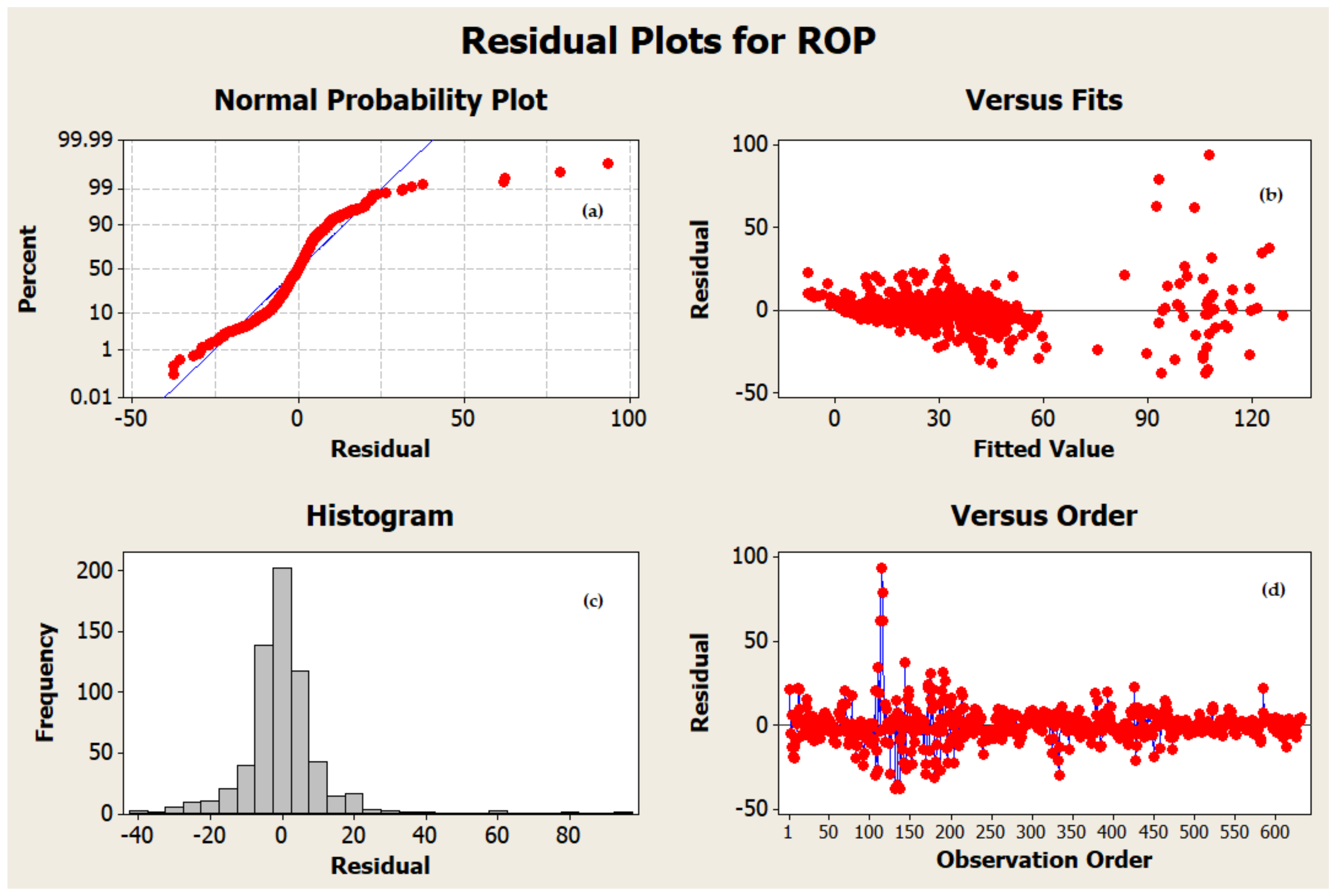
The CCD design was utilized for the generation of fitting Equation (17) with a face-centered configuration where alpha was one. The ten input variables were considered as factors that were coded in two levels (1, −1). There were 128 cube points, 10 center points, and 20 axial points present in the developed CCD design with a total of 158 base runs. The quadratic equation of RSM contains controllable input factors and uncontrollable factors. These uncontrollable or predefined factors such as Measured Depth (DT), AZ, etc., were held as constant, as they cannot be altered. The objective function of ROP developed using RSM is given below.

$$\begin{array}{l}f(x)=21.61\times x_2+12.337\times x_4-15.34\times x_5+37.57\times x_9-0.1554\times x_{10}-17.67\times x_1^2+2.55\times x_2^2-0.1699\times x_3^2-2.325\times x_4^2\\ +3.35\times x_5^2-2.6398\times x_9^2-11.72\times x_1{x}_2-7.04\times x_1{x}_2-7.04\times x_1{x}_3-12.437\times x_1{x}_9-16.11\times x_2{x}_7+1.84\times x_2{x}_9-8.67\times x_4{x}_6\\ -3.767\times x_4{x}_8+0.0564\times x_4{x}_{10}-7.391\times x_5{x}_9+9.156\times x_5{x}_8+0.0723\times x_5{x}_{10}-59.62\end{array}$$

(17)

where f(x) is the approximate objective function of ROP along with other drilling variables as shown in Table 2. This ROP Equation (17) shows predictor variables in the quadratic fitting equation. The R², adjusted R², and predicted R² for the above-mentioned objective function are 84.41%, 82.68%, and 81.23% respectively, as given in Table 6. Adjusted R² shows the goodness of fit for the developed regression model. Less difference between R² and adjusted R² shows that important predictors were selected for fitting a quadratic polynomial of RSM. Contours and 3D surface plots were also generated to have a better visualization of the effects of various predictor variables with ROP, as shown in Figure 8 and Figure 9. These plots were helpful for the manual search of optimal points in case of a lower number of input variables. Surface plots and contour plots are utilized to understand and determine the desirable values of the target variable by varying the input variables. Contour plots are two-dimensional representations where all the points having the same response (or target) values are connected. The surface plot provides three-dimensional visualization of the interaction between response (target variable) and input variables. These plots are helpful in the manual estimation of optimum values for the model parameters when the number of input variables is low. However, it is very difficult to find the global maximum point manually in our case, as the number of input variables is 10 (Equation (17)). Therefore, ABC and GA are used [26,27] to optimize Equations (16) and (17).

The significance level of 5% was used while developing an objective function for ROP (Equation (17)). It has been reported the 5% significance level balances Type 1 and Type 2 error during hypothesis testing of any regression coefficients [45,46]. The correctness of the developed ROP objective function was validated by analysis of variance (ANOVA) test, as shown in

Table 11. Results of the ANOVA test for significant terms in the ROP Equation (17) utilized in this study *.

Source	DF	Sum of Squares	Mean Square	F-Value	p-Value	T-Value
Model	63	10.29	0.1633	48.74	0.00	0.000
$x_2$	1	0.98	0.1022	30.51	0.00	5.524
$x_4$	1	0.013	0.013	3.94	0.047	1.986
$x_5$	1	0.0158	0.0157	4.71	0.030	−2.169
$x_9$	1	0.02	0.02	5.97	0.015	2.444
$x_{10}$	1	0.0020	0.00204	0.61	0.036	−1.779
$x_1\times x_1$	1	0.022	0.020	5.98	0.015	−2.445
$x_2\times x_2$	1	0.1132	0.1132	33.77	0.000	5.811
$x_3\times x_3$	1	0.0001	0.00005	0.02	0.897	−0.129
$x_4\times x_4$	1	0.0139	0.0139	4.15	0.042	−2.038
$x_5\times x_5$	1	0.0243	0.0243	7.24	0.007	2.691
$x_9\times x_9$	1	0.0343	0.3433	10.24	0.001	−3.200
$x_1\times x_2$	1	0.1493	0.1493	44.57	0.00	−6.676
$x_1\times x_3$	1	0.0154	0.0154	4.61	0.032	−2.146
$x_1\times x_9$	1	0.0027	0.00271	8.09	0.005	−2.844
$x_2\times x_7$	1	0.1153	0.1153	34.4	0.000	−5.865
$x_2\times x_9$	1	0.0206	0.0206	6.15	0.013	2.480
$x_4\times x_6$	1	0.0157	0.01565	4.67	0.031	−2.161
$x_4\times x_8$	1	0.0134	0.0133	4.01	0.046	−2.002
$x_4\times x_{10}$	1	0.0206	0.0206	6.15	0.013	2.480
$x_5\times x_9$	1	0.1299	0.1298	38.75	0.000	−6.225
$x_5\times x_9$	1	0.0534	0.05303	15.82	0.000	3.978
$x_5\times x_{10}$	1	0.0137	0.01366	4.08	0.044	2.019

* Table 11 contains the ANOVA analysis of significant terms only, while insignificant terms that fail in the significance test of 5% are eliminated to reduce the redundancy in Equation (17).

. This test demonstrates that coefficients satisfy 5% significance level criteria. All the terms having P values higher than the significance level were eligible for the null hypothesis, which resulted in zero value of coefficient terms and was eliminated from the ROP regression equation. Table 11 shows all the coefficients having lower P values. A T-test was also performed to validate the significance of the regression coefficient of the ROP function. There are several missing interaction terms in the ROP objective function such as BT*BT, BT*BS, etc. due to their higher P values. The developed Equation (17) has been optimized using the ABC algorithm available in the python beecolpy 2.1 packages based on Karaboga and Basturk [22]. Figure 10 shows residual plots of errors resulted from the developed ROP objective function using RSM. Figure 10 is composed of four residual plots for the developed ROP objective function using RSM, which are explained below.

(a)

A normal probability plot is used to verify the normal distribution of residual data. Ideally, the fitted data should follow a straight line. However, it was found to be not true for the studied drilling datasets, as the trend did not follow a straight line. This verifies the complexity of the real field drilling datasets.

(b)

Histogram of residuals plot provides details about data skewness or outliers. The skewness is confirmed by a long tail in one direction; however, if a bar is distant away from the other bars, it indicates noise or outlier in the residual data. In the studied drilling datasets, no such problem with data distribution has been found.

(c)

The residual vs. fits plot checks the constant variance of the residual. It plots the fitted values on the x-axis and residual on the y-axis and verifies the model assumption of the random distribution of residuals as well as constant variance. It is expected that the data points should lie randomly on both sides of the 0 line with no pattern [26,27], which is true in our case.

(d)

The residual vs. order plot checks whether residuals are uncorrelated or not. These graphs are generated to inspect the goodness of fit of fitting Equation (17) and ANOVA test. Normally, a model residual must lies randomly on both sides of the centerline with no patterns, which is true for our drilling data as well. The generated ROP Equation (17) has satisfied all the required standard conditions to be a good fitting equation (approximate function/objective function).

The developed Equation (17) has been considered as an ROP objective function. During the optimization process, Equation (17) was maximized using ABC with upper and lower bounds, as shown in Table 10 according to the following steps:

(a)

Initialize the search boundaries using the range of parameters provided in Table 10 and code Equation (17) as an objective function;

(b)

Adjust the other parameters of ABC (colony size = 50, scouts = 0.5, iterations = 100, min_max = ‘max’, nan_protection = True). Here, the size of the colony determines bees in the algorithm. Half of its values represent food sources, employed bees, and onlooker bees;

(c)

The algorithm returns a global optimal solution for the ROP objective function along with the locations of food sources or possible solutions (local maxima);

(d)

Record the values of ROP and other variables including BT.

Table 12. Comparative analysis of drill bit selection results for the test geological zones.

Bit Selection	Models		Zone 1	Zone 2	Zone 3	Zone 4	Zone 5
[47]		ANNs	3	5	4	3	8
[6]/[9]		ANNs and GA	3	5	6	7	8
Proposed approach		RSM and ABC	1	5	6	7	8
Actual BT Data			1	5	6	7	8

,

Table 13. Comparison of drill bit selection results based on cost per foot calculation for different approaches.

Target Zones	ANNs Predicted	Cumulative CCF $/ft	ANNs and GA	Cumulative CCF $/ft	Proposed Approach	Cumulative CCF $/ft
Zone 1	3	50	3	50	1	24
Zone 2	5	25	5	25	5	25
Zone 3	4	456	6	396	6	396
Zone 4	3	50	7	50	7	50
Zone 5	8	64	8	64	8	64

and

Table 14. The optimum value of input drilling variables for certain depths of target zones using a combination of RSM and ABC.

DT	WOB	TQ	RPM	SPP	MW	BT	ROP
Zone 1	3.72	0.01	90	62.6	1.03	1	47.4
Zone 2	3.64	16.67	176	247.3	1.39	5	40.35
Zone 3	16.01	21.8	178	279.3	1.22	6	10.56
Zone 4	6.94	31.25	139	193.8	1.41	7	11.61
Zone 5	6.87	22.28	140	205.9	1.4	8	27.54

contain the optimum values of drilling variables and BT for target formations along with cost per foot.

5. Discussion

The selection of suitable drill bits is essential for a successful drilling operation to minimize the overall wellbore cost and increase the efficiency of the drilling operations. In this study, an alternative approach has been investigated for drill bit selection using RSM and ABC combination. RSM has been utilized to develop an objective function for ROP and to determine optimum values of drilling control variables using ABC. Ten drilling variables were considered as input variables for the development of the ROP objective function, namely; DT, BT, BS, WOB, RPM, TQ, MW, IN, AZ, and SPP. Three nearby Norwegian wells’ data have been considered for testing the proposed approach of drill bit selection. The five geological zones of well C were utilized for the testing of data-driven drill bit selection techniques, as shown in Table 12 and Table 13. Figure 5 shows the generalized schema of the proposed approach for drill bit selection. The developed objective Equations (16) and (17) for ROP were optimized with the upper and lower bounds provided in Table 10 to obtain the optimum value of BT and ROP. Table 12 contains the bit types selected on the optimum ROP values using different data-driven approaches. ANN has wrongly predicted the drill bit types for zones 1, 3, and 4; however, when combined with GA, its drill bit selection error reduces to zone 1 only.

ANN has been reported to have a tendency to get stuck in local minima, which is why it failed to predict the correct bit type for certain target formations [19,48]. When ANN is combined with GA, the optimization task is handled by GA, which is a strong optimizer and converses to the correct BT except in zone 1, as compared to actual BT. Equations (16) and (17) are multimodal equations developed through high-dimensional data comprised of large local optimal points. Therefore, detecting a globally optimum solution in the search space is a difficult task. In the case of GA, sometimes, premature convergence may happen due to strong selection pressure imposed by the selection operator and crossover operator if the initial population lacks desirable diversity. However, ABC utilizes a stochastic search technique that is good at maintaining diversity and escaping local optimal stagnation. Table 12 shows that the proposed RSM and ABC combination has precisely estimated the bit types for five target geological zones. Here, information about actual drill bits used in the real field for drilling the wells has been taken as a standard reference for comparison in Table 12. Table 14 contains the optimum values of drilling variables acquired through RSM and ABC combination at different target depths. Moreover, the performance of drill bits selection techniques must be compared based on the drilling cost involved in the drilling operations. It might be possible that the GA-suggested BT for zone 1 is more suited for an applied bit. Therefore, the cost per foot analysis should be done for each drill bit to check the economic feasibility of suggested drill bit types.

The oil and gas industry has direct as well as indirect impacts on the global economy, which decides the fate of the sustainable development of human beings. The revenue generated by the oil and gas drilling sector alone was approximately 3.3 trillion U.S. dollars, which was roughly 3.8% of Global Gross Domestic Product (GDP) in 2019 by IBISWorld data [49]. The upstream drilling sector is also known as the exploration and production industry (E&P industry). However, the contribution of industries midstream and downstream of the petroleum sectors was never included in the above-said data; otherwise, the GDP percentage share of the petroleum industry would be much greater. Therefore, any economical and innovative technological development in the E&P industry will have a global impact. This will also encourage a global economy that influences human sustainability, as clearly mentioned in the sustainable development goals of the UNDP.

The type of drill bits utilized in any drilling operation has an economical influence on the overall drilling operation. The drilling cost has a direct relationship with ROP and the running life of the drill bit that is needed to be minimized. Polycrystalline diamond compact (PDC) drill bits were primarily utilized for drilling the Norwegian wells considered in this study. Nearly 10–40% of the dryhole well cost is found dependent on the PDC drill bit [7]. The PDC bit life fluctuates with its design parameters such as cutter distribution, type of gauge protection material, etc., whereas design parameters such as nozzle placement, cutter shape, PDC type, etc. directly vary the bottom hole ROP drastically [7]. Therefore, the selection of a suitable BT is essential for the minimization of associated drilling costs. The selection performance of different data-driven approaches has also been compared based on cost per foot analysis. The prices of drill bits were identified from the manufactures catalogs. The totality of trip time and connection time was expected to be 6 hours per 1000 ft. Equation (1) has been utilized to perform the cost per foot analysis of the predicted drill bit. Table 13 shows the computed cost per foot results for five target zones of well C based on drill bits selected through different data-driven approaches. Figure 11 shows that the selection of the bit for five target drilling zones by ANN and GA combination and proposed approach has given nearly similar types of drill bits and cost per foot except for zone 1. The proposed approach has given a lesser cost per foot value for zone 1 as compared to ANN and GA combination, as shown in Table 13. Table 14 shows the optimum value of input drilling variables for certain depths of target zones using a combination of RSM and ABC. Therefore, the proposed RSM and ABC combination is found to be more reliable than ANN-based drill bit selection models and can also be utilized for the drill bit selection purposes. Moreover, these models are case-specific, as well as data-dependent in nature, and require calibration for other fields.

Mostly, PDC drill bits have been utilized along with roller cone bits for the drilling of the Norwegian wells considered in this study. These bits are widely applied in offshore conditions due to various benefits such as to reduce tripping time, to drill in non-hydrating formations, to achieve high RPM and ROP in directional drilling, etc. However, PDC bits are sensitive to fragile and soft formations as in the case of Volve wells considered in this study. These wells comprise softer rock formations that contain fine to medium sandstone, some interbedded claystone, siltstone, and limestone stringers, marl, argillaceous laminations, etc., as shown in Table 1. Soft, fragile, and fractured rock formations affect the stability of PDC bits with a large reduction of the bit life. Recently, hybrid drill bits (e.g., Kymera) have been developed that combined the properties of conventional PDC bit and roller cone bit types [49,50,51]. These hybrid bits seem to be a good solution for drilling problematic wellbore sections while maintaining the stability of drilling operations. It may be possible that the drilling cost per foot has been reduced more if hybrid drill bits are employed for drilling the Norwegian wells considered in this study.

6. Conclusions

UNDP promotes economic innovations that lead to the growth of any industrial sector. In this work, attempts have been made to develop a more reliable technology for drilling optimization and cost reduction of drilling operations. RSM and ABC combination has been proposed to select drill bit type based on the optimum values of ROP. RSM has been utilized for the development of the ROP objective function, which is further optimized using ABC to find the optimum values of ROP. The optimum values of operational variables are also determined in this research work for drilling the target formations. A comprehensive study has been done to test the efficacy of the proposed method with the existing ANN, ANN, and GA for drill bit selection and drilling optimization. The analysis of the results obtained leads to the following conclusions.

• This study provides an alternate intelligent approach for bit selection based on optimum values of ROP.
• The proposed drill bit selection approach is found to be more accurate than the ANN-based prediction of drill bit types.
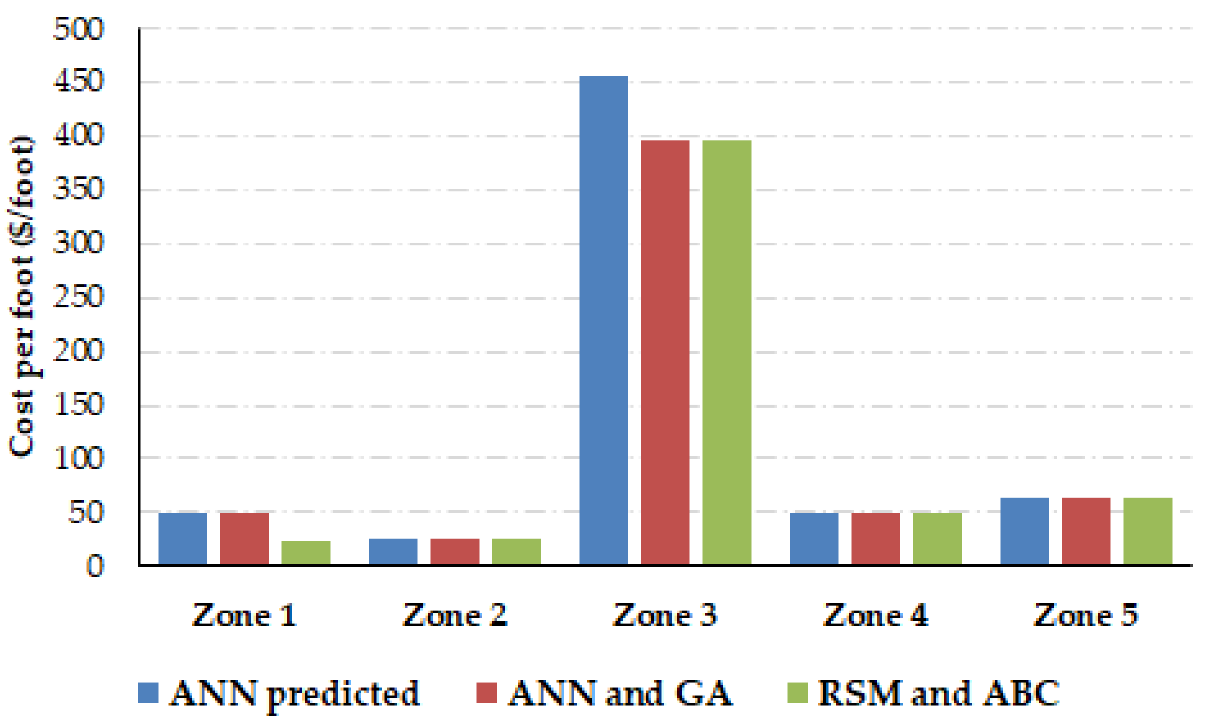
• The combination of RSM and ABC provides a more reliable bit selection modeling approach as compared to ANN based on cost per foot comparison.
• The prediction correlation coefficient of the RSM objective function is found to be 81.23%, while 85.5% has been found for ANN during the estimation of ROP.
• The ROP objective function developed through RSM is less complex than the ANN-based objective function due to the absence of an exponential function.
• ANN requires more computational cost for the development of the ROP function and its optimization.
• These models are case-specific data-dependent models and require calibration for other field data.
• The proposed data-driven approach has presented optimism for the sustainable development of more efficient, robust, reliable, and economical technology that has shown potential for drilling optimization and cost reduction.

This research work indicates the potential of coupled intelligent techniques for the estimation and optimization of drilling variables. Using the proposed model, drilling engineers can effectively reduce the overall time and expenses that a company invests in a field by smartly selecting the optimum parameters of any newly planned oil and well.

7. Code Source

The results have been generated through Matlab 2019, MiniTab 2016, and python toolbox Geneticalgorithm 1.0.1. and beecolpy 2.1.

References

1. Bahari, A.; Seyed, A.B. Drilling cost optimization in a hydrocarbon field by a combination of comparative and mathematical methods. Pet. Sci. 2009, 6, 451–463. [Google Scholar] [CrossRef] [Green Version]
2. Teale, R. The concept of specific energy in rock drilling. Int. J. Rock Mech. Min. Sci. Geomech. Abstr. 1965, 2, 57–73. [Google Scholar] [CrossRef]
3. Perrin, V.P.; Mensa-Wilmot, G.; Alexander, W.L. Drilling index-a new approach to bit performance evaluation. In Proceedings of the SPE/IADC Drilling Conference, Amsterdam, The Netherlands, 4–6 March 1997. [Google Scholar]
4. Yιlmaz, S.; Demircioglu, C.; Akin, S. Application of artificial neural networks to optimum bit selection. Comput. Geosci. 2002, 28, 261–269. [Google Scholar] [CrossRef]
5. Bahari, M.H.; Bahari, A.; Moharrami, F.N.; Naghibi-Sistani, M.B. Determining Bourgoyne and Young model coefficients using genetic algorithm to predict drilling rate. J. Appl. Sci. 2008, 8, 3050–3054. [Google Scholar] [CrossRef]
6. Edalatkhah, S.; Rasoul, R.; Hashemi, A. Bit selection optimization using artificial intelligence systems. Pet. Sci. Technol. 2010, 28, 1946–1956. [Google Scholar] [CrossRef]
7. Momeni, M.S.; Ridha, S.; Hosseini, S.J.; Meyghani, B.; Emamian, S.S. Bit selection using field drilling data and mathematical investigation. In IOP Conference Series: Materials Science and Engineering; IOP Publishing: Bristol, UK, 2018; Volume 328, p. 012008. [Google Scholar]
8. Momeni, M.; Hosseini, S.J.; Ridha, S.; Laruccia, M.B.; Liu, X. An optimum drill bit selection technique using artificial neural networks and genetic algorithms to increase the rate of penetration. J. Eng. Sci. Technol. 2018, 13, 361–372. [Google Scholar]
9. Abbas, A.K.; Assi, A.H.; Abbas, H.; Almubarak, H.; Al Saba, M. Drill Bit Selection Optimization Based on Rate of Penetration: Application of Artificial Neural Networks and Genetic Algorithms. In Proceedings of the Abu Dhabi International Petroleum Exhibition & Conference, Abu Dhabi, United Arab Emirates, 11–14 November 2019. [Google Scholar]
10. Hightower, W.J. Proper selection of drill bits and their use. In Proceedings of the SPE Mechanical Engineering Aspects of Drilling and Production Symposium, Fort Worth, TX, USA, 20–23 March 1964. [Google Scholar]
11. Bourgoyne, A.T., Jr.; Young, F.S., Jr. A multiple regression approach to optimal drilling and abnormal pressure detection. Soc. Pet. Eng. J. 1974, 14, 371–384. [Google Scholar] [CrossRef]
12. Rabia, H.; Farrelly, M.; Barr, M.V. A new approach to drill bit selection. In Proceedings of the SPE European Petroleum Conference, London, UK, 20 October 1985; pp. 20–22. [Google Scholar]
13. Fear, M.J.; Meany, N.C.; Evans, J.M. An expert system for drill bit selection. In Proceedings of the SPE/IADC Drilling Conference, Dallas, TX, USA, 15–18 February 1994. [Google Scholar]
14. Uboldi, V.; Civolani, L.; Zausa, F. Rock strength measurements on cuttings as input data for optimizing drill bit selection. In Proceedings of the SPE Annual Technical Conference and Exhibition, Houston, TX, USA, 3–6 October 1999. [Google Scholar]
15. Bybee, K. A New Approach for Drill-Bit Selection. J. Pet. Technol. 2000, 52, 27–28. [Google Scholar] [CrossRef]
16. Bilgesu, H.I.; Al-Rashidi, A.F.; Aminian, K.; Ameri, S. A new approach for drill bit selection. SPE Eastern Regional Meeting, London, UK, 17–19 October 2000. [Google Scholar]
17. Kůrková, V. Kolmogorov’s theorem and multilayer neural networks. Neural Netw. 1992, 5, 501–506. [Google Scholar] [CrossRef]
18. Villarrubia, G.; De Paz, J.F.; Chamoso, P.; De la Prieta, F. Artificial neural networks used in optimization problems. Neurocomputing 2018, 272, 10–16. [Google Scholar] [CrossRef]
19. Polikar, R. Pattern Recognition. Wiley Encyclopedia of Biomedical Engineering; John Wiley & Sons, Inc.: New York, NY, USA, 2006. [Google Scholar]
20. Muthiah, A.; Rajkumar, R. A comparison of artificial bee colony algorithm and genetic algorithm to minimize the makespan for job shop scheduling. Procedia Eng. 2014, 97, 1745–1754. [Google Scholar]
21. Alqattan, Z.N.M.; Abdullah, R.A. Comparison between Artificial Bee Colony and Particle Swarm Optimization Algorithms for Protein Structure Prediction Problem. Lect. Notes Comput. Sci. 2013, 827, 331–340. [Google Scholar]
22. Karaboga, D.; Basturk, B. A powerful and efficient algorithm for numerical function optimization: Artificial bee colony (ABC) algorithm. J. Glob. Optim. 2007, 39, 459–471. [Google Scholar] [CrossRef]
23. Myers, R.H.; Khuri, A.I.; Walter, H.C., Jr. Response Surface Methodology. Technometrics 1989, 31, 137–157. [Google Scholar]
24. Montgomery, D.C. Design and Analysis of Experiments; John Wiley & Sons, Inc.: New York, NY, USA, 2014. [Google Scholar]
25. Hecht-Nielsen, R. Kolmogorov’s mapping neural network existence theorem. In Proceedings of the IEEE First International Conference on Neural Networks, San Diego, CA, USA, 21–24 June 1987; Volume 989, pp. 11–14. [Google Scholar]
26. Box, G.E.P.; Wilson, K.B. On the Experimental Attainment of Optimum Conditions. In Breakthroughs in Statistics. Springer Series in Statistics (Perspectives in Statistics); Kotz, S., Johnson, N.L., Eds.; Springer: New York, NY, USA; Morgantown, WV, USA, 1993. [Google Scholar]
27. Myers, R.H.; Montgomery, D.C.; Anderson-Cook, C.M. Response Surface Methodology: Process and Product Optimization Using Designed Experiments; John Wiley & Sons. Inc.: New York, NY, USA, 1995; pp. 134–174. [Google Scholar]
28. Karaboga, D. An Idea Based on Honey Bee Swarm for Numerical Optimization. Technical Report-tr06, Erciyes University, Engineering Faculty, Computer Engineering Department. 2005. Available online: http://citeseerx.ist.psu.edu/viewdoc/download;jsessionid=E32274EB05825D919807935CF722606F?doi=10.1.1.714.4934&rep=rep1&type=pdf (accessed on 29 October 2020).
29. Zhao, Y.; Noorbakhsh, A.; Koopialipoor, M.; Azizi, A.; Tahir, M.M. A new methodology for optimization and prediction of rate of penetration during drilling operations. Eng. Comput. 2020, 36, 587–595. [Google Scholar] [CrossRef]
30. Nozohour-leilabady, B.; Fazelabdolabadi, B. On the application of artificial bee colony (ABC) algorithm for optimization of well placements in fractured reservoirs; efficiency comparison with the particle swarm optimization (PSO) methodology. Petroleum 2016, 2, 79–89. [Google Scholar] [CrossRef] [Green Version]
31. Koopialipoor, M.; Ghaleini, E.N.; Haghighi, M.; Kanagarajan, S.; Maarefvand, P.; Mohamad, E.T. Overbreak prediction and optimization in tunnel using neural network and bee colony techniques. Eng. Comput. 2019, 35, 1191–1202. [Google Scholar] [CrossRef]
32. Ghaleini, E.N.; Koopialipoor, M.; Momenzadeh, M.; Sarafraz, M.E.; Mohamad, E.T.; Gordan, B. A combination of artificial bee colony and neural network for approximating the safety factor of retaining walls. Eng. Comput. 2018, 35, 647–658. [Google Scholar] [CrossRef]
33. Ahmad, A.; Razali, S.F.M.; Mohamed, Z.S.; El-shafie, A. The application of artificial bee colony and gravitational search algorithm in reservoir optimization. Water Resour. Manag. 2018, 30, 2497–2516. [Google Scholar] [CrossRef]
34. Ravasi, M.; Vasconcelos, I.; Curtis, A.; Kristi, A. Vector-acoustic reverse time migration of Volve ocean-bottom cable data set without up/down decomposed wavefields. Geophysics 2015, 80, S137–S150. [Google Scholar] [CrossRef] [Green Version]
35. Equinor Website Database. Available online: https://www.equinor.com/en/how-and-why/digitalisation-in-our-dna/volve-field-data-village-download.html (accessed on 17 August 2020).
36. Hornik, K.; Stinchcombe, M.; White, H. Multilayer feedforward networks are universal approximators. Neural Netw. 1989, 2, 359–366. [Google Scholar] [CrossRef]
37. Ripley, B.D. Statistical aspects of neural networks Networks and Chaos: Statistical and Probabilistic Aspects. Chapman Hall 1993, 50, 40–123. [Google Scholar]
38. Paola, J.D. Neural Network Classification of Multispectral Imagery. Master’s Thesis, The University of Arizona, Tucson, AZ, USA, 1994. [Google Scholar]
39. Wang, C. A Theory of Generalization in Learning Machines with Neural Applications. Ph.D. Thesis, The University of Pennsylvania, Philadelphia, PA, USA, 1994. [Google Scholar]
40. Masters, T. Practical Neural Network Recipes in C++; Morgan Kaufmann: Burlington, VT, USA, 1993. [Google Scholar]
41. Kanellopoulos, I.; Wilkinson, G.G. Strategies and best practice for neural network image classification. Int. J. Remote Sens. 1997, 18, 711–725. [Google Scholar] [CrossRef]
42. Kaastra, I.; Boyd, M. Designing a neural network for forecasting financial and economic time series. Neurocomputing 1996, 10, 215–236. [Google Scholar] [CrossRef]
43. Zorlu, K.; Gokceoglu, C.; Ocakoglu, F.; Nefeslioglu, H.A.; Acikalin, S. Prediction of uniaxial compressive strength of sandstones using petrography-based models. Eng. Geol. 2008, 96, 141–158. [Google Scholar] [CrossRef]
44. Demuth, H.; Beale, M.; Hagan, M. Artificial Neural Networks & Genetic Algorithms User’s Guide. Revis. Matlab Program. 2007, 5. Available online: http://cda.psych.uiuc.edu/matlab_pdf/nnet.pdf (accessed on 18 January 2021).
45. Lindenmayer, D.; Burgman, M.A. Monitoring, assessment, and indicators. Pract. Conserv. Biol. 2005, 401–424. [Google Scholar] [CrossRef]
46. Schlotzhauer, S. Elementary Statistics Using JMP; SAS Publishing: Cary, NC, USA, 2007. [Google Scholar]
47. Hou, B.; Chen, M.; Yuan, J. Optimization and Application of Bit Selection Technology for Improving the Penetration Rate. Res. J. Appl. Sci. Eng. Technol. 2014, 8, 179–187. [Google Scholar] [CrossRef]
48. Tewari, S.; Dwivedi, U.D. Ensemble-based Big Data Analytics of Lithofacies for Automatic Development of Petroleum Reservoirs. Comput. Ind. Eng. 2018, 128, 937–947. [Google Scholar] [CrossRef]
49. Ibisworld Website Database. Available online: https://www.ibisworld.com/industry-insider/search/?query=GDP (accessed on 3 December 2020).
50. Pessier, R.; Damschen, M. Hybrid bits offer distinct advantages in selected roller-cone and pdc-bit applications. Spe Drill. Complet. 2011, 26, 96–103. [Google Scholar] [CrossRef]
51. Tewari, S.; Dwivedi, U.D.; Biswas, S. A Novel Application of Ensemble Methods with Data Resampling Techniques for Drill Bit Selection in the Oil and Gas Industry. Energies 2021, 14, 432. [Google Scholar] [CrossRef]
Figure 1. The architecture of the Artificial Neural Network (ANN) investigated in this study.
Sustainability 13 01664 g001
Figure 2. The layout of face-centered design (alpha = 1) for central composite design (CCD).
Sustainability 13 01664 g002
Figure 3. A flowchart of Response Surface Methodology (RSM) and Artificial Bee Colony (ABC) for the development and optimization of the Optimum Penetration Rate (ROP) equation.
Sustainability 13 01664 g003
Figure 4. Flowchart of the Artificial Bee Colony paradigm [28].
Sustainability 13 01664 g004
Figure 5. A generalized schema of the proposed approach for drill bit selection.
Sustainability 13 01664 g005
Figure 6. Location of Volve oil and gas field in the North Sea [34].
Sustainability 13 01664 g006
Figure 7. The prediction performance of optimal ANN architecture [10-18-1] for developing an ROP objective function (a) Regression plot, (b) Mean square error (MSE) plot, and (c) Error plot.
Sustainability 13 01664 g007aSustainability 13 01664 g007b
Figure 8. Contour plots show interactions of different input variables visualized in the 2D plane for Equation (17). (Example: In Weight on bit (WOB) × Measured depth (DT) subplot, WOB is on the y-axis, whereas DT on the x-axis.).
Sustainability 13 01664 g008
Figure 9. Surface plots for ROP objective function generated through the RSM technique. These plots help visualize the interactions between various input variables. These are graphical visualizations of the fitted ROP shown in Equation (17).
Sustainability 13 01664 g009
Figure 10. Residual plots of errors from developed ROP objective function using RSM. (a) Normal probability plot is used to verify the normal distribution of residual data (b) Histogram of residuals provide details about data skewness or outliers’ presence. (c) The residual vs. fits plot confirms the constant variance of residual. (d) The residual vs. order plot checks whether the residuals are uncorrelated or not. These graphs are generated to inspect the goodness of fit of fitting Equation (17) and the ANOVA test.
Sustainability 13 01664 g010
Figure 11. The comparison of cost per foot calculated for five target geological zones. The ANN and Genetic Algorithm (GA) combination has given a similar cost per foot as compared to the proposed RSM and ABC approach, except in zone 1. In zone 1, RSM and ABC have given lower cost per foot results than the ANN and GA combination.
Sustainability 13 01664 g011