Article

Decision-Making Rules and the Influence of Memory Data

1
Department of Economics, Faculty of Economics, University of South Bohemia in Ceske Budejovice, Studentska 13, 370 05 Ceske Budejovice, Czech Republic
2
Department of Urban Engineering, Faculty of Civil Engineering, VSB—Technical University of Ostrava, Ludvika Podeste 1875/17, 708 00 Ostrava-Poruba, Czech Republic
*
Author to whom correspondence should be addressed.
Sustainability 2021, 13(3), 1396; https://doi.org/10.3390/su13031396
Submission received: 11 December 2020 / Revised: 8 January 2021 / Accepted: 18 January 2021 / Published: 29 January 2021
(This article belongs to the Special Issue Sustainable Decision Making in Civil and Construction Engineering)

Abstract

:
The problems that decision-makers face can escalate under imbalances, turbulent development, risks, uncertainties, disasters, and other influences. The development of processes in technical and economic structures is generally considered complex and chaotic, and it usually expands into innumerable dynamic influences. The paper focuses on the evaluation of the decision criteria choice structure, such as the factual cause of the consequences (e.g., future threats, opportunities, chances, occasion). It offers a graphical vision of the future forecast. It draws attention to prevention and prophylaxis versus criterion-generated time–space (TS). The paper deals with the question: Is it possible to choose and recommend the right time and place of process activities? The paper formulates a positive answer and illustrates a range of consequences. Developed activities (investment, production, etc.) take place in a defined TS; over time, they create new time-series states and expand the space by defining processes as a time series of activities. In a broader context, the article deals with the issue of the lifecycle of decision rules (dynamic proposal of opportunities) as the first step of decision making, i.e., the decision about the existence of opportunity. On the one hand, it respects static applications based on equilibrium states, while on the other hand, it draws attention to the need for a dynamic view of turbulent, dynamic, chaotic, and nonlinear phenomena.

1. Introduction

The modern debate about sustainability encompasses the application of commonly used complex simulations that are considered useful to predict tomorrow’s world opportunities with good accuracy [1,2,3,4]. Some authors, such as [5], claimed that the economics and financial industry and risk management, in particular, need more advanced and detailed mathematical models [6,7,8]. Others, especially representatives of the Austrian School of Economics [9], have long denied the appropriateness of mathematical methods for economic and technical economic research. The approach has deep roots and, in part, good and simplistic arguments.
Tarasov aptly summarized the differences in opinion conducted in the 20th century and late 19th century by stating that modern economics was born in the marginal revolution and the Keynesian revolution. These revolutions led to the emergence of fundamental concepts and methods in economic theory, which allow for the use of differential and integral calculus to describe economic phenomena, effects, and processes. At present, the new revolution, which can be called memory revolution, is taking place in modern economics [10]. In this context, we are addressing the development of discipline dynamics economic [11,12,13] and the narrow profiles of the methods and theories used to date [1,14,15]. The works of Mandelbrot are still interesting contributions (see [16,17]). Statistical models challenged by the authors in [18] emphasize the need to capture unexpected events, and the authors proposed the use of fractals. Fractals are, in Mandelbrot´s approach, tied to the geometrical criteria. The approach presented here shapes decision rules (DRs) as a logical construct (based on verbal formulated premises and valid in time). Therefore, DRs form the decision space [19], and moreover, they concretize the admissibility of potential solutions (e.g., variants, alternatives). The DRs fulfil the dual role of being judges (for the past) on the imaginary time axis of the simulation calculus and being legislators (for the prospect of the future).
Fractal features appear in almost any economics data and any modern project realization. However, all real projects have strict dynamic behavior in time. Most calculations about such a project are based on deterministic equilibrium, such as in the design, financing, use and innovation. The need of a more sophisticated theoretical approach is desirable, and more practical experience is necessary. There are many different project realizations. The general theory and analysis are, therefore, extremely difficult. An economical dynamic of fractals is still developing. The path and direction of the theory may already be known, but an effective application tool is still missing.
The initial state is determined by assigning a starting position for a cell in time sequence t = 1, 2, 3, …, m as the utility value u(t) [20]. Any new generation step is created by following a logical decision rule. The rule determines the new states of the current short-term ex post situation in its past neighborhood.
The idea of a 2D cellular automaton (CA) was originally discovered in the 1940s by Stanislaw Ulam and John von Neumann at the US Los Alamos National Laboratory and presented as Conway’s Game of Life (see [21] for more). The idea was subject to significant academic debate, through which scholars developed discrete simulation models that are studied in mathematics, physics, and theoretical biology, which can be found in Wolfram’s Approaches to Complexity Engineering, as seen in [22,23]. However, the idea’s applications in an economic context have been fragmented into many professional fields [17,18]. Furthermore, the author in [10] classified, in his review, the development of dynamic models in economics into five stages: autoregressive fractionally integrated moving average (ARFIMA) [24], fractional Brownian motion, econophysics, deterministic chaos, and mathematical economics. The affinity of Turing-completeness (for simulating data manipulation sets) to CA was published by Wolfram in [25], who pointed out CA applications in many science areas.
A decision rule in this paper is a deterministic function that generates a structure of opportunity actions over a problem-oriented time–space. The processing is devoted to aspects that are passable for IT deterministic simulation calculations.
This paper focuses on the interpretation of CA/fractals and on the economic context, that is, by means of combinational logic devoted to the formation of the decision space. The difference from Mandelbrot’s approach lies in the formation of criteria. Mandelbrot forms criteria on the geometric basis. The general explanation about the decision process is given in the second subsection of Section 3 (i.e., Analysis).
The decision process and paper structure are based on three steps:
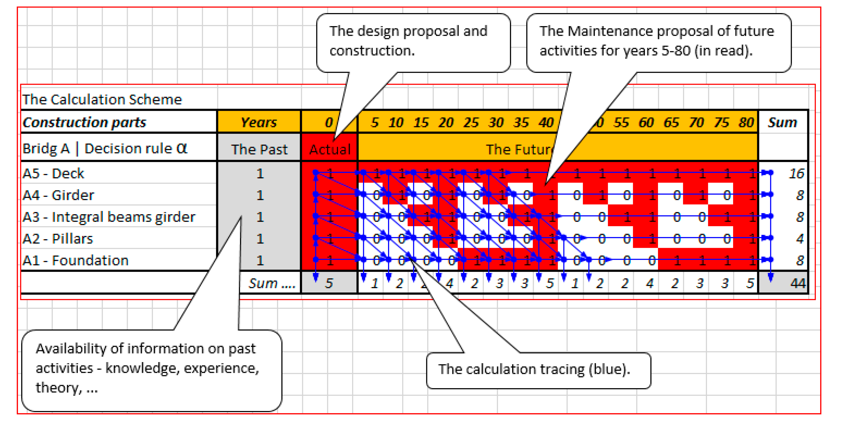
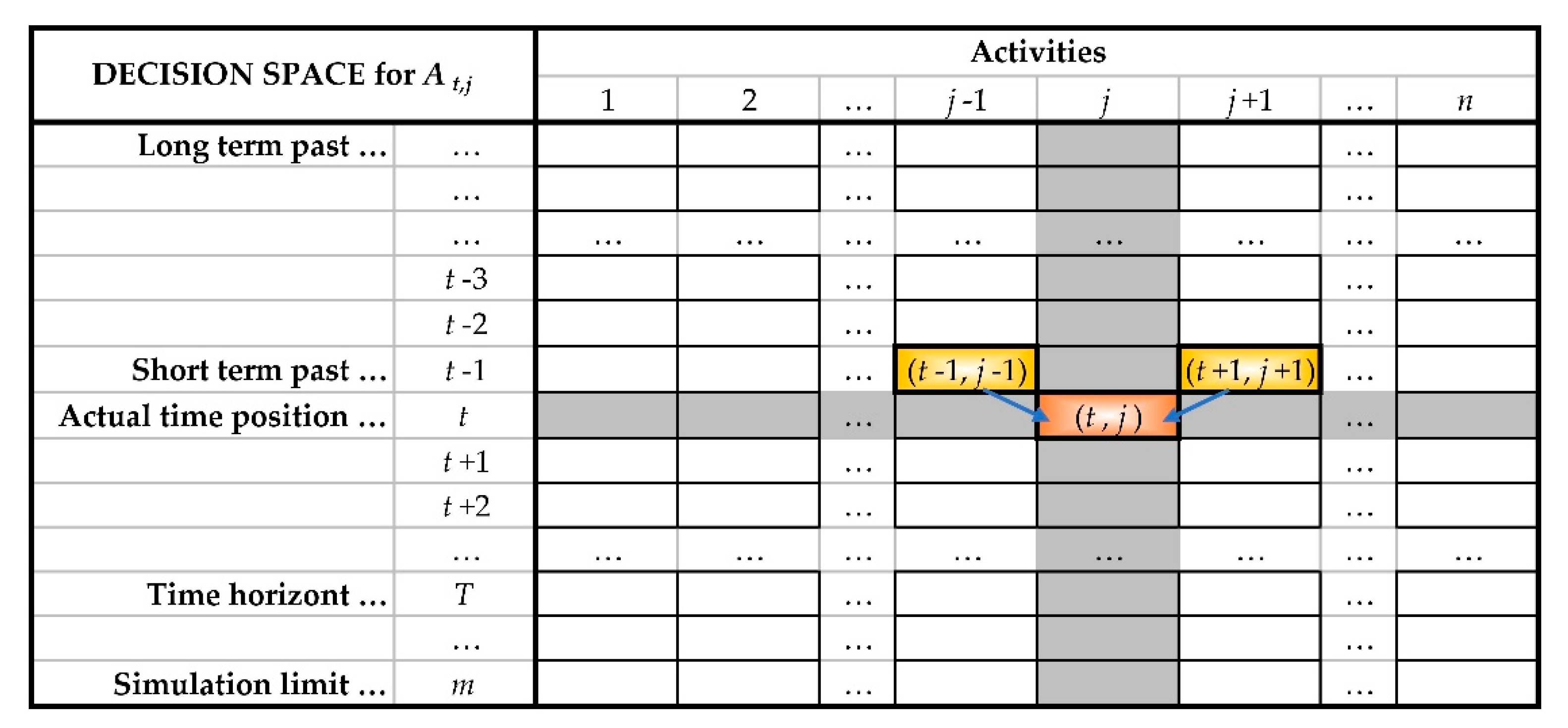
  • Space for decision making (i.e., formation): Most of the arguments for fractal dynamic modelling are included in Section 2.2. Figure 1 shows the long-term application of a decision rule in the dynamic decision space SA = (A, t), where A is a set of activities At, j located in time t and their affiliation j to SA for tracking opportunities as (0;1) or (N;Y), or expressed as colors. The choice or activity is determined by professional regulation (standards, laws, guideline, etc.);
  • Decision making: Opportunities in SA are calculated using decision rules Dopportunities = {(Drules, Mdata)|SA}. A look at the calculation of opportunities is offered in Section 3. It deals with a basic decision rule grounded on a general, verbally formulated logical requirement. Comparing memory Mdata dependence is the topic of the paper. This problem is treated as the productivity of the Drule in Section 3 as well as Figure 2 and Figure 3;
  • Decision evaluation: Utility is the final step addressed in the article. Section 4 addresses the need for valuation opportunities. More implementation is offered in Section 5. Both the space for decision making and the decision making itself create an introduction to practical application in the Appendix A example. The evaluation of the utility is also listed in the illustrative example as an evaluation of the frequency of maintenance and renewal interventions. The extensive construction of utility functions is, however, a separate problem in the design of decision rules.
The decision process is constituted of (a) decision-making rule D [26], (b) a decision-making space S [23], (c) the decision data structure (M, memory data [27,28,29], which are data about past decisions), and (d) the evaluation of the decision space positions (U, utility set) [30].

2. Materials and Methods

2.1. The Decision Process—Decision Rule Horizon and Decision Rule Memory

The decision criterion (i.e., the decision rule) generates (or forms) the decision space. In the present paper, the economic applications are illustrated as a 2D space (t,j) for economic decision-making in time (sequence t = 1, …, m) as one dimension and activities (j = 1, …, n) as the second dimension of S. The calculation of the benefit of activity Atj in the decision space is assessed in terms of potential utility utj (i.e., it is awarded utility, e.g., 0/functional award (value); or 0/1; false/true; impossible/possible; keep/sell; white/red; −100/+500). The assessment in decision-making requires calculation evaluation. The evaluation creates values u(t,j), and these represent the economic interpretation [30,31]. The result is a matrix U, which covers the decision space, as presented in (1), that is, they are ex post values for the present state data. With advancing calculation time steps, the data of activities of the present Atj become data about the past At-τ,j, and are read as history and memory
U = [ u 1 , 1 u 1 , j u t , 1 u t , j u m , 1 u m , j u 1 , n   u t , n u m , n ]
where Atj is an activity j adjusted (implemented) in time t.
The decision rules, D, have a broad interpretation in this article (see the formulation in (2) for more details). The D rules can be defined either on a geometric basis (e.g., [16]), as a mathematical function [25], or as a statistical dataset [17]. This paper prefers a logical structure, economic interpretation, rationality, or aesthetic principles, among other things. In most practical applications, the rudimentary decision criteria shape the space in time, which is described here as a dynamic development. In a multifaceted socioeconomic environment [32,33], which we perceive as a dynamic process [34], we recognize decision rules (criteria) as a dominant element. The paradox is that even if an economic decision criterion is held steady over time, this changes the opportunities inside the decision-making space (see Figure 1a and compare with Figure 1b–d).
For example, it is true that during different periods, the same set of rules can lead to significantly different results. Specifically, rules may lead to a certain outcome in the context of long-term decision making, represented here as DLong. The time horizon T is significantly distanced from the initial t (i.e., T >> t), and shows various outcomes; this is seen in the context of short-term decision-making (DShort), where T = 1 or 2, or decisions are typically developed without time horizons, that is, T = 0. In economics, decision rules typically serve the pragmatic purpose of selecting a goal, setting preferences, selecting options, identifying alternatives, representing regulatory requirements, and other acts of predominantly short-term execution. The substantive impact on decisions is the fuzzy time horizon (short-, medium-, long-term). Economic decision criteria are predominantly based on defined logical conditions and mostly relate to a general experience.
Figure 1 shows how different the decision-making situation is in the relatively short-term time horizon (see Figure 1a,b) and for the long-term horizon (see Figure 1c,d). The visual differences are already striking: the short-term and long-term time horizon T evokes the “experience” that the rule for long-term decision-making creates a more significant density of application (i.e., “opportunities”).
One further important component is to be noted, namely, the memory of data [35]. In an economic context, a decision rule is related to ex post events, which are events with an evaluated history. In other words, the data memory is fixed to time (tτ). If decision criteria use data from the past to develop an excluded decision rule with memory, the assumption is typically made to implement the decision rule D based on a general formula, such as
IF ((D is true) then (evaluation Atj as utj = 0) else (evaluation Atj as utj = 1))
Every space element (t,j) may host activities Atj or remain empty. The decision rule distinguishes the suitability of location (t, j) for activity Atj. The utility can be evaluated as
utj = F(Atj|N)
where N is the selected neighborhood of the cell (t, j) and F is an arbitrary functional specifying the utility value for the (t, j) location. The economic interpretation of the neighborhoods are logical rules or administrative rules, legislation, environmental requirements, etc. In this paper, the analysis will simply refer to the calculation based only on a set of ex post data.
If the analysis focuses on the current state t = 0 and a reflection on the last past outcome τ as −1, or the last and penultimate result −1 and −2, etc., then it is said to consider the decision rule memory. The delay τ defines the range of memory and specifies (or influences) the phenomenon of the actual economic opportunity. This is represented graphically in Figure 1a–d. More details are given in Figure 2 and Figure 4. The short-term memory decision rule Dα is set as
IF((At−1,j−1 = At−1,j+1) then ut,j = 0 ⇒ field fill white else ut,j = 1 ⇒ field fill red
The color fill in Equation (4) simplifies the interpretation of Equation (2). The decision rule Dα is described as follows: When the last past period of both neighboring activities is successful, or when both activities are unsuccessful, no activity will be developed (white in the graph). The success of one of the neighboring activities in the past leads to the decision to implement one’s own activity. Figure 1a and Figure 2 have an identical initial simulation step. Further steps in Figure 1a–d show how long the horizon can change the structure of opportunities.
The illustration is given in Figure 1 (see Figure 3 and Figure 4 for more) and verifies the demand for more comprehensive research of decision rules.
In a broader view, we touch on the sensitive issue of long-life dynamics decision-making. It is visible from practice that there is a gap in the methods used to date. This is mainly reflected in tenders and projects with a long lifecycle, innovative projects, etc. Some questions that emerge as follows: (a) to what extent D is bound to the space SA; (b) to what degree are the benefits of U related to the functionality of D over time; (c) to which extent are the benefits of U are related to the link between D and historical (or memory) data; (d) to what extent is the lack of opportunities in SA (opportunities = 0) an obstacle to the development of the investigated technical–economic projects.

2.2. Research Question

The essential question is to what extent the construction of the decision rules influences the decision space and how intensively the data memory might influence the decision space. If the data history significantly shapes the decision space, there is a need to give careful consideration to this information. Stored data about the past are relevant for the present and might shape the decision space for the future.
Real data sources typically represent a technical economic process. For this analysis, we substitute a real process with CA. Furthermore, we identify the process as a fractal created on the basis of decision rules, extending the interpretation of [17]. It is assumed that the decision rule is implemented in a process, according to Expression (2), whereby this expression is a schematic model that can be applied to most activities in a technical–economic context, as per Figure 2.
Typical examples of interpretations of this analytical approach are life-governing rules that factually form a dynamic process. The sequence (i.e., the dynamic) of time and space is often considered defined by increasing completeness and efficiency. Accordingly, the main focus of this paper is to shed light on this.
Specifically, the paper develops a response to the following questions:
  • To what extent does the construction of the decision rules influence the decision space? This question reflects the considerations posed by [36];
  • How intensively might the data memory influence the decision space?
We see a dispersion of activities (investment, knowledge, etc.) as a result of the technical–economic rules (built-in technicalities or prescribed functional properties). Section 3 further deals with the issue of evaluation of the decision criteria in detail. This concept is applicable in many areas of development, innovation, construction, and architecture. The present paper applies this concept to the development of technical–economic processes that represent regional development, investment, etc. [6,37]. An illustrative example is given in Appendix A, Figure A2, i.e., the horizontal form of the decision space SA (read as SBridge maintenance), time steps 1–80.
The frequency of activities applied acts across time and per space of activities, as shown in Figure 2 and comparison to Figure 3, Figure 4 and Figure 5. The spread of activities in time depends on the decision rule and the use of historical data. The rule states that if the former time period was successful for one of the next neighboring activities in the immediate past, the decision makers need to build on the success while in the current position (that is, initial innovation occurs, knowledge is gained, investment follows, along with further development [38]). It is believed that memory, information, and experience from the last time period are sufficient for making a decision in the current time period [29]. In other words, the memory of the recent time period is the primary enabler of decision-making for the current period.
The interpretation of memory data is frequently related to computer science and operation systems in practice [27]. In the context of the simulation described above, we could speak about dynamic time-dependent data and data memory that is constantly refreshed.
Business managers, engineers, and architects will face this dilemma at many points in time, and they make a decision based on the best information available to them at that point in time [39]. The decision maker has to evaluate whether the information is complete, unbiased, and authentic. The quantity and quality of data available for decision making become important for them to understand the quality of the decision made. Due to the uncertainty [40,41] of information, which is inherent to the dynamic situation of the business or other practical contexts, a decision maker has to evaluate an uncertain outcome, which is considered a random variable [42].

2.3. Research Hypotheses

Three hypotheses can be developed to provide insight into the mechanism of decision making and data memory:
  • Decision rules change the operational decision space for the decision maker depending on the time horizon of the memory used, e.g., (t − 1), (t − 2);
  • The spread of activities in time is conditioned by the chosen DR.
    Comment: Industries and companies typically request stable regulation rules (in terms of regulatory, economic, ecological, or political rules, etc.), mostly without calculating the expected opportunities and their usefulness;
  • The DR simulation utility characterizes the decision criterion both for (a) a schedule of opportunities and (b) individual activities over time.

3. Analysis

The previous chapter dealt with the broader context of the effects of the decision rule on the decision space and the potential of its use. An illustrative example is shown in Figure 3. To select suitable solutions (variants, alternatives of DR), it is necessary to quantify the use of created opportunities, their expiration, and intensification [43]. The DRC used for the simulation of opportunities in Figure 2 applies its basic graphical form, as given in Figure 3.
Using the decision rule, the structure of implementation opportunities to achieve reasonable utility outcomes needs indicators.
The opportunities created are unquestionable. These are the intensities of opportunities measured by the frequency of their occurrence in individual time periods and individual activities forming the monitored project. They are the main evaluation content in Figure 2 [44].
The sums of utilities in the time (applied activities in time sequence) are shown in the right part, by a vertical graph. They characterize the use of activities (individual utilities, in the sense of Equation (3), are evaluated as 1), introduced for simplicity: applied activity = utility = 1. Similarly, the frequency of application of individual activities in the simulation time sequence is characterized by the graph at the bottom of Figure 2. Fluctuation in the utilities is provided by individual activities.
The immediate characteristics that are offered for quantification are as follows:
(a)
The total space S□ for the involved activities in the project:
S□ = 1023 activities × 512 time horizon = 523,776 potential interactions;
(b)
Total application space after Dα activation:
S∆ = 1023/2 × 512 = 261,888 potential interactions;
(c)
Total space after Dα simulation:
S▲ = 19,171 proposed interactions according to Dα.
From the comparison of the defined space of activities SΔ and the total potential of concentrated activities S□, we obtain (SΔ/S□ = 261,888/523,776); we interpret this as the percentage of the potential of allocated activities. We see that for the limit purposes in Dα, it is possible to use only 50.00% of the total interaction space. The Dα reduces the available space for SΔ application in Figure 2 to 7.32%; the simulation of opportunities on the basis of Dα reduces these spaces further—fractal simulated opportunities use 3.66% of S□ space.
The economic consequences and limits for different applications are significant in this context of dispersion. Application deals with opportunity and possibility. These are mostly investments, innovations, the application of inventions, patents, development strategies, and more [45]. The usability of opportunity at the level of percentage units is only associated with the usability of invested resources. In the current interpretation, we move on to the level of generalizing and reasoning. The effort to improve the productivity and efficiency of the decision-making rule through deeper binding to data obtained from the historical past has its limits.
In the following text, the article deals with the question of the consequences of connecting the criteria with historical data (as in statistical data, databases of knowledge, experience, evaluated experiments, and others).
The economic consequences and limits for different applications are significant in this context of dispersion. Application deals with opportunities and possibility. These are mostly investments, innovations, the application of inventions, patents, development strategies, and more. The usability of opportunity at the level of percentage units is only associated with the usability of invested resources. In the current interpretation, we move onto the level of generalizing and reasoning. The effort to improve the productivity and efficiency of the decision-making rule through a deeper binding to the data obtained from the historical past has its limits.

3.1. The Influence of Data Memory (i.e., Data History) on Decision Rules

The creation of the process structure in Figure 2 is based on the use of the most recently available ex post data (t − 1); the decision rule Dα, described earlier, is summarized in Table 1, and the simulation results shows and clarifies Figure 3. Similarly, Figure 4 is based on the (t − 2) memory scheme in Table 2, and the last (t − 3) of Table 3 results in Figure 5.
We need to distinguish the data forms of the past and current data used in the decision rule and the future (data ex ante). Suppose that Equation (2) represents a real process (such as a project of investment or innovation benefits or the spread of knowledge) that occurs in the market environment and causes the placement of quantitative parameters. This is interpreted as a market product and is presented in Figure 2 as blue-filled spaces.
To have a practical interpretation in mind, it can be assumed that Figure 1, Figure 2, Figure 3 and Figure 4 show the decision rules, which are the basis for a potentially successful strategic decision (e.g., investment or another economic asset). The calculation conditions are detailed in Table 1, Table 2, Table 3 and Table 4. The purpose is to draw attention to the possibility of creating computational decision rules based on a text source or verbal formulation of decision rules. The formulations, which cannot be converted into a decision rule, most likely contain a formulation or interpretation defect. Simultaneously, with the transfer of the text to the decision rule, it is expedient to assess the question regarding to what extent it is desirable to use (incorporate) data with memory (statistical data, experience, and more) into the decision rules.
The usefulness or benefit created by means of the decision rules α, β, and γ as a tree structure is presented in particular time periods in Figure 2, Figure 4 and Figure 5. Details of the structure are offered in the frequency graphs on the right side and bottom of these figures. It is possible to distinguish the cycle and the excessive frequency values and volatility in some time periods for the decision rules α, β, and γ. The decision rules differ across time series and enable a comparison of decision rule implementation efficiency.
It can be seen in Table 4 that, for example, productivity for At,j is the highest for decision rule α.

3.2. Comparison of Decision Rule Productivity

The decision rules influence the outputs of the process under investigation and its utility (productivity). The decision rules based on ex post data (t − 1), (t − 2), (t − 3) explained in Table 1, Table 2 and Table 3 form the utility (productivity) of activities At,j. The shape of the decision outcome is evident from the dispersion of activities in Figure 2, Figure 4 and Figure 5.
The summarized results are concentrated in Table 4. The range S points out the ability to spread the benefits of activities At,j in simulating the opportunities in the defined space SΔ. We see that the utilization dispersion indicates the volatility in (g) in the obtained data of Table 4.
The three research hypotheses formulated in “Section 2.3” find their confirmation in the simulations of Figure 2, Figure 4 and Figure 5. Dependencies are not linear; they have long-term dynamic development. The use of decision rules on memory leads to a narrowing of the application space (Table 4, columns of default data in columns (b), (d), and subsequent).
The usefulness or advantage created by the decision rules α, β, and γ as a tree structure is shown in time (simulation steps) in Figure 2, Figure 4 and Figure 5. Details of the structure are shown in the frequency graphs on the right and bottom of these figures. It is possible to distinguish high or low values of frequency and high volatility in some periods for decision rules α, β, and γ. Decision-making rules differ in time steps and allow for a comparison of the implementation effectiveness of the decision-making rules.
It can be seen, for example, that the spread of application opportunities (productivity) is the highest for the decision rule α. The volatility in simulation steps changes over time. Under such circumstances, significant follow-up economic and technical consequences may occur.

3.3. Productivity Efficiency of Decision Rules α, β, and γ

The summary of the results based on decision rules α, β, and γ is given in Table 4. Results are attained on the basis of long-term simulation. A number of observations can be made:
  • Decisions based on the data memory narrow the range of information and space available for potential actions Aj (opportunity of economic response), as seen in Figure 2, Figure 4 and Figure 5;
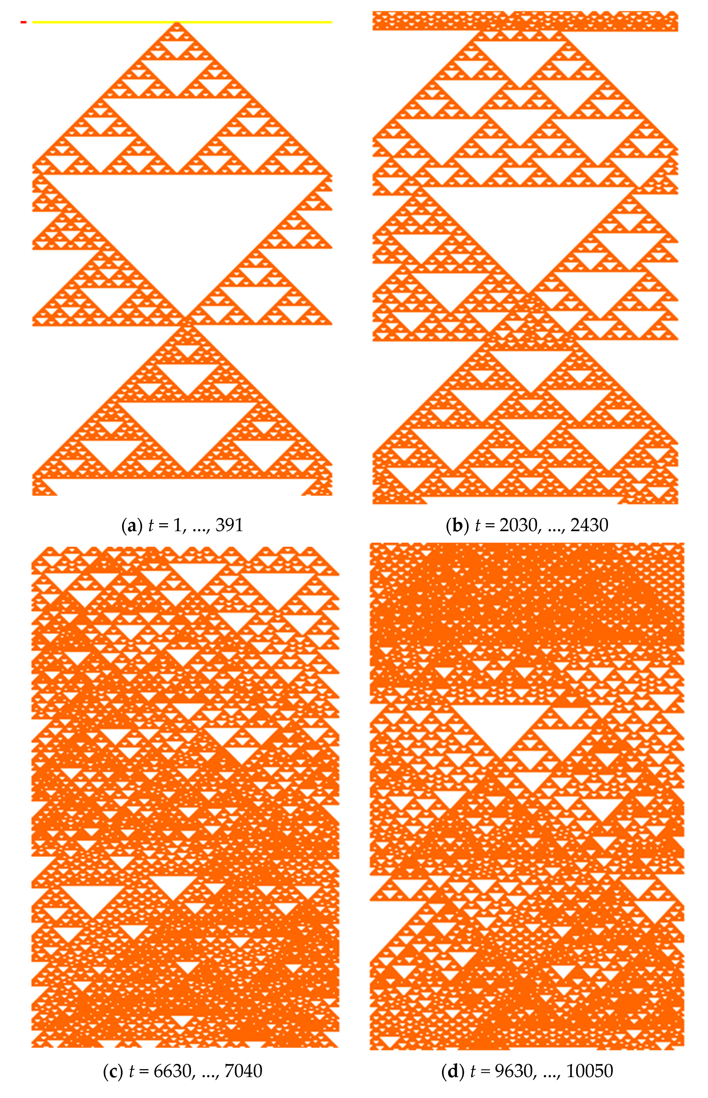
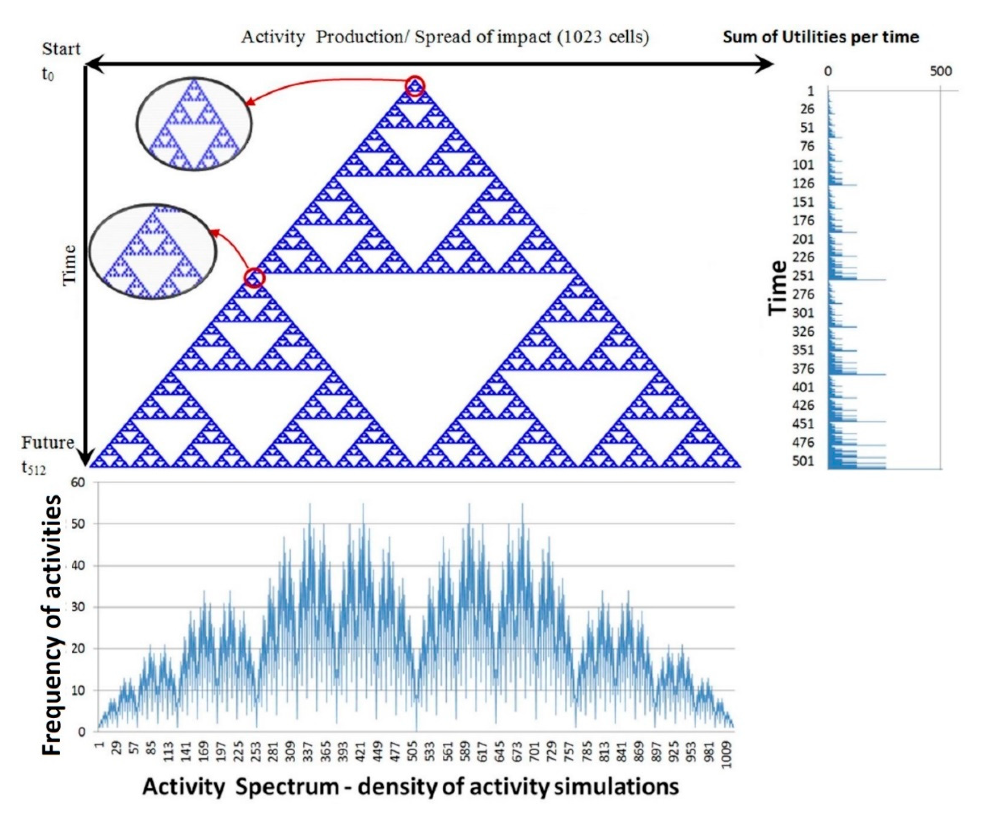
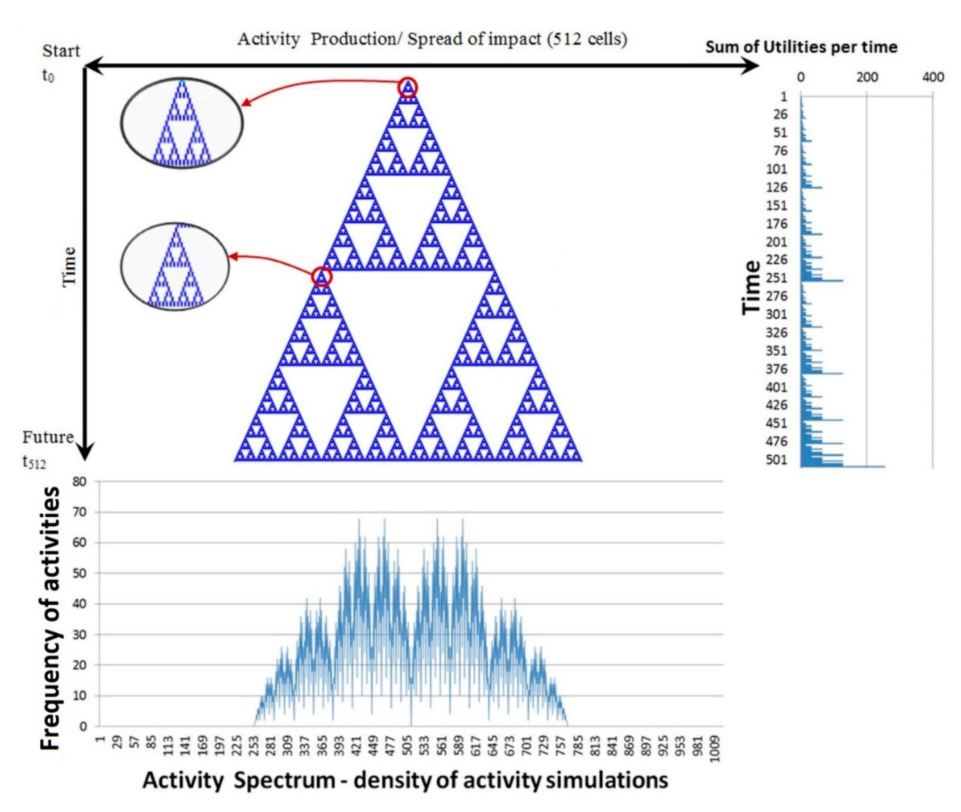
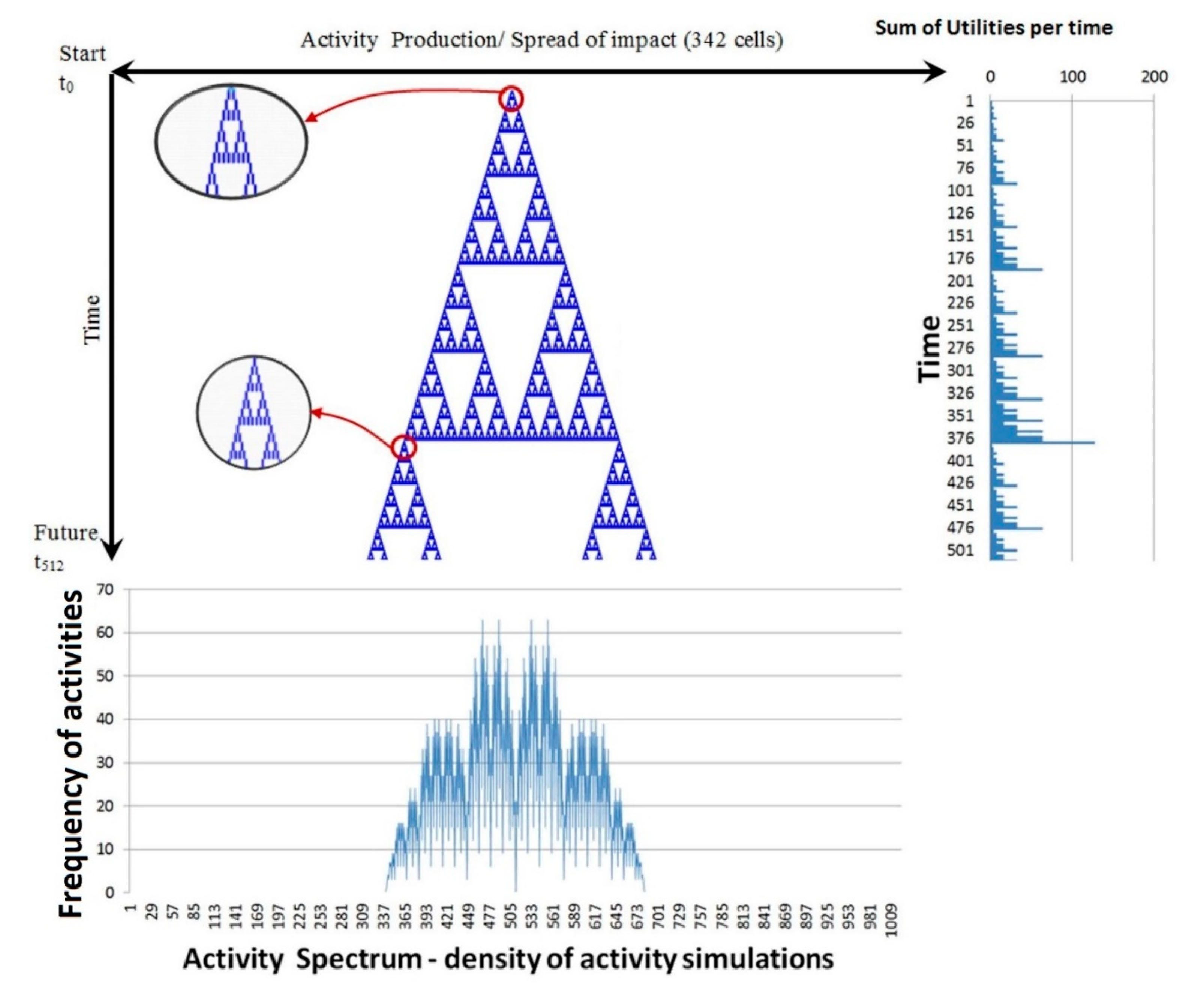
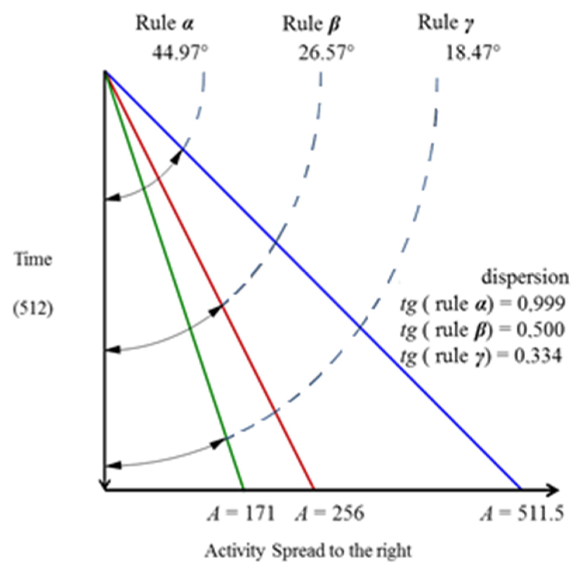
  • The inclusion of a backward (historical data) time (t − 1) into the decision criterion Dα (t − 1) in Figure 2 leads to a decrease in opportunities to 50.0% of the influenced space (261,888 units), compared to space available (523,776 units). The reduction of 131,072 of 523,776 units is 25% for decisions on the basis of two time periods (t − 2), as well as the reduction on the basis of data (t − 3) to 16.72% (523,773 units to 87,552) for Dγ on the basis of data (t − 3); details are in Table 4 and Figure 2, Figure 4 and Figure 5. The inclusion of one or more backward time steps into the decision criterion leads to narrowing the influenced implementation area (S(t − 1) in Table 4, column (e) 19,683 as 100%) to 13,123; this is 68.4% for (t − 2), and 43.1% for (t − 3). Further comparisons are given in Table 4;
  • The spread of the impact of decision rules of activities Aj slows down at a rate of tangent α; (indicator) is given as tg(Dα) = 0.999 to tg (Dβ) = 0.500 and tg(Dγ) = 0.334.
On this basis, conclusions can be drawn about the avoidance of risk [46,47] or conservative behavior. The economic consequences are a decrease in productivity for an ongoing process, as well as the reduction in opportunities as a future economic response.

4. Discussion

The above analysis provides the answer to fundamental questions regarding decision processes in real life. An example of a maintenance schedule is given in Appendix A. Some important questions are as follows:
  • Does a decision process really act in a homogeneous decision space?
    The decision space is not homogenous for the rules modelling real-life situations, which were examined in this paper as decision rules (α, β, and γ). A time range of productive periods for Dαβγ exists, as do a range of unproductive time arrangements, which exhibit a lack of utility [48];
  • Does the lack of homogeneity of the decision space affect the environment for implementing decisions?
    The decision space creates bubbles that cover substantial areas of the decision space. These bubbles indicate the absence of productive activity. Moreover, the decision space affects the utility (productivity) of subsequent time periods and parallel-running activities in the long term. To some extent, these are affected activities Aj, which can cause a long-term negative domino effect, that is, the productive space at various subsequent time steps is a sensitive structure of opportunities. The knowledge about decision consequences, which helps to choose an appropriate action in an appropriate time step, helps to generate a higher utility [49];
  • To what extent is the decision in the decision layers (t − 1), (t − 2), (t − 3), etc., affected by decisions in previous layers (i.e., the decision history)?
    Binding Dαβγ to data with history causes significant changes in the decision space; it changes the range of effects that are available (see Figure 6). The pattern of productive activity is exhibited in Figure 3 and Figure 4. This clarifies the significant modifications across the decision layers;
  • To what extent is the decision in the decision layers (t − 1), (t − 2), (t − 3), etc., able to influence decisions in future layers?
  • The pattern of active (productive) space in Figure 2, Figure 4 and Figure 5 shows a strong sensitivity of Dαβγ to ex ante development. Because of this, the Dαβγ exhibits similarity.

5. Conclusions

Decision making is one of the crucial tools supporting progress in any discipline. The paper argued that the prerequisite of successful development is to know the expected chances of future development. In this sense, we presented the idea about opportunities. This is an inverse to the concept of missed opportunities. Figure 1 illustrates the consequences, the long-time application of a relatively simple decision rule. The decision opportunity was introduced as Dopportunity = {(Drule; Mdata)|SA } and is a surrogate for term prognosis, plans, prospect, etc.
A preview of the long-simulated simulation segment (a, b, c, d) suggests the following:
  • A long-term life of activities included in the created decision-making space;
  • The “thickening” opportunities over time;
  • The existence of bubbles without application opportunities and their displacement during the lifecycle of the decision rule;
  • Creating application cycles of opportunities.
Information on the consequences of the application of the decision criterion has a long-term strategic character. This creates an essential support of economic and technical disciplines.
Decision-making rules in common practice are based on the experience and knowledge created in the past. They compose the future based on the knowledge of the past. This issue was addressed in particular by the investigation of the examples in Section 2 and Section 3 of this article.
We appreciate this point for situations in which transparent, mostly long-term valid databases dominate. Empirical confirmation is generally a necessary condition, but not without sufficient exceptions [50,51]. The values created by large national units should comply with the principles of evaluation, based on the idea of sustainable economic growth [52] and the need for return on investment, capital, and invention, to create long-term benefits [53,54]. However, many carefully selected activities do not achieve their goals [55,56]; for instance, the completion deadline was exceeded, the solution sustainability failed, or the externality costs unexpectedly rose [57].
Consequently, it is often misunderstood that the dynamics of the application opportunities for the intended economic and technical capital goods are dominant [58,59]. The calculation of opportunities is often overlooked, and it either did not occur or internal or external influences were excluded. The discussed fact is that future developments are difficult to detect. This argument is not full-fledged because of the current absence of tools for evaluating the decision criteria, and their application in processes depicting the space in which activities (such as large capital-intensive projects) are to be invested.

Author Contributions

V.B. and M.T. provided the core idea, collected the data, wrote the manuscript and statistically analyzed the data. F.K. revised and constructively commented on the paper, checked the formal correctness. All authors have read and agreed to the published version of the manuscript.

Funding

The work was supported by funds for Conceptual Development of Science, Research and Innovation for 2021 allocated to VSB–Technical University of Ostrava by the Ministry of Education, Youth and Sports of the Czech Republic.

Institutional Review Board Statement

Not applicable.

Informed Consent Statement

Not applicable.

Data Availability Statement

Publicly available datasets were analyzed in this study. This data´s links can be found in the references.

Conflicts of Interest
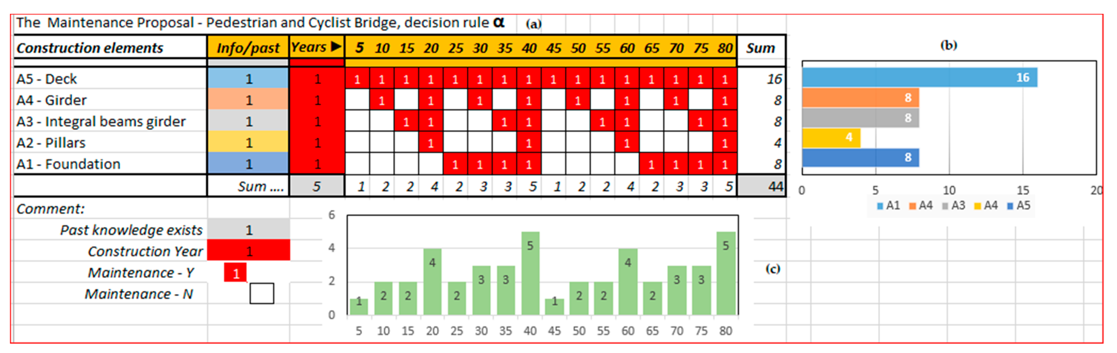
The authors declare no conflict of interest. The funders had no role in the design of the study; in the collection, analyses, or interpretation of the data; in the writing of the manuscript, or in the decision to publish the results.

Appendix A

An application example in a fractal environment is seen in the maintenance and renewal of a pedestrian–cyclist bridge. Engineering projects are known as investment-intensive. At the same time, they also have high costs for maintenance, renewal, and modernization during their lifetime. It is these issues that are neglected or ignored at the time of investment. The correct selection of construction variants or alternatives is essential. Figure A1a,b illustrates the two projects of the integrated column. The presented pedestrian and cyclist bridge case study follows the scheme in Figure 3, and it shapes the space for maintenance application. The individual activities of the bridge construction (i.e., structural elements) are the foundation (A1), pillars (A2), integral beams girder (A3), girder (A4), and deck (A5). The example brings the presentation closer to the usual time schedule scheme; the time axis is horizontal. In Figure A3, the information is divided into the past (information on the feasibility of individual structural elements), present (implementation), and future (forecast of the design of time intervals for the implementation of cyclic maintenance and renewal).
The study has its specific background in a number of bridge structures such as footbridges in the Czech Republic. There was also a reclassification of these structures to the category of “emergency”. Photographs are shown in Figure A1a,b. They illustrate the new design solutions chosen for the new installations in Prague–Troja and Pisek.
Figure A1. Transverse profile of the pedestrian and cyclists’ bridge. (a) Prague–Troja in 2020, (b) Pisek-Pleskot pedestrian and cyclist bridge in 2018. (a) Reproduced with permission from S. Vojtasek, Construction journal; published by KONSTRUKCE Media Plc., 2020.; (b) Reproduced with permission from H. Malik, Construction of the Year 2019; published by Triangl Corp., 2019.
Sustainability 13 01396 g0a1
Although the project of the new solution focuses on technical functionality and the authorial effect, it is in the public interest that the costs of the entire lifecycle are efficient per unit time. The economics of evaluating technical solutions, i.e., the applied rules of current decision practice, are mostly based on (empirical) cost budgets. This has to do with short-term horizons, as in the project is limited to the design and construction (the pedestrian bridge Prague–Troja m2 cost ca. EUR 5859 and length meter ca. EUR 23,437; Pisek–Pleskot bridge, ca. 5809 EUR/m2, and ca. 17,428 EUR/m).
The paper offers an alternative as a dynamic fractal life cycle. Figure A2 shows the spreadsheet segment and comments. The construction structure is simplified. Most EU national economies work with a standardized work breakdown structure (WBS). The reason for using a WBS is to eliminate the cost control risks of construction projects. A summary of the calculation using the decision rule α is shown in Figure A3.
Figure A2. The calculation scheme—MS Excel; Bridge activities A1–A5 and time steps for t = 80.
Sustainability 13 01396 g0a2
The main result of the case study is the creation of a maintenance and renewal schedule based on the fractal structure created by the decision rule α. The individual maintenance cycles are a fractal structure (Figure A3). Moreover, activities A1–A5 create maintenance cycles with a fixed time and structure of the activities. They are visualized as bar graphs. A total of 44 maintenance interventions are included. The bridge deck in A5 requires 16 hits (as shown in the horizontal density graph, Figure A3 in the right part). Similar information about technical lifecycle is presented in a vertically oriented density graph for individual time periods of maintenance.
Figure A3. Calculation results: (a) maintenance time schedule, (b) construction elements maintenance density (service-life 80 years, in right), (c) for two technical life cycles, 2 × 40 years.
Sustainability 13 01396 g0a3
A clear segmentation of the individual maintenance cycles is shown separately in Figure A4. The time sequences are particularly noticeable.
Figure A4. The construction elements A1–A5—Maintenance cycles; displayed as two technical life cycles (1–8), (8–16).
Sustainability 13 01396 g0a4
The issue of maintenance cycles is summarized in Table A1. Attention is given to the high concentration of maintenance needs for activities A5 and A4. For the first cycle of technical life, it is necessary to spend 36.36% + 18.18% of interventions. In this case, it is 54.54% of maintenance activities.
Table A1. The issue of maintenance cycles.
ActivityCycleDensity *Density **
MaintenanceYearsLC 80: %Σ 44: %
(a)(b)(c)(e)
A5—Deck520.00%36.36%
A4—Girder1010.00%18.18%
A3—Integral beams girder2010.00%18.18%
A2—Pillars205.00%9.09%
A1—Foundation2510.00%18.18%
Note: * Maintenance density %; life cycle (LC) 80 years. ** Maintenance density %, construction elements. Applied (44 times) in LC 80 years.
However, the actual engineering standard of the project consists of innovations of elements A3, A2, and A1. Although disproportions can be further supported by cost analysis, the possibilities of project modifications can already be deduced from the assessment of the fractal structure.

References

  1. Forrester, J. World Dynamics; Wright-Allen Press: Cambridge, MA, USA, 1971. [Google Scholar]
  2. Lorenz, E.N. Deterministic nonperiodic flow. J. Atmos. Sci. 1962, 20, 130–141. [Google Scholar] [CrossRef] [Green Version]
  3. Miao, J. Economic Dynamics in Discrete Time; MIT Press: Cambridge, MA, USA, 2014; p. 710. ISBN 978-0-262-02761-8. [Google Scholar]
  4. Nguyen, M.H.; Nguyen, V.Q. Dynamic Timing Decisions under Uncertainty: Essays on Invention, Innovation and Exploration in Resource Economics; Springer: Heidelberg/Berlin, Germany, 2013; p. 198. ISBN 978-3-540-57649-5. [Google Scholar]
  5. Trees of Life. Philosophy of Biology, 1st ed.; Griffiths, P.E., Ed.; Kluwer Academic Publishers: Dordrecht, The Netherlands, 1992; pp. 1–13. ISBN 978-94-015-8038-0. [Google Scholar]
  6. Schumpeter, J.A. The Theory of Economic Development; Harvard University Press: Cambridge, MA, USA, 1934. [Google Scholar]
  7. Kuda, F.; Teichmann, M.; Proske, Z.; Szeligova, N. Modern approaches of facility management in the management and maintenance of underground services. In Proceedings of the 17th International Multidisciplinary Scientific Geoconference, SGEM 2017, Albena, Bulgaria, 29 June–5 July 2017; Volume 17, pp. 279–288. [Google Scholar] [CrossRef]
  8. Schumpeter, J. Business Cycles: A Theoretical, Historical, and Statistical Analysis of the Capitalist Process; McGraw-Hill Book Company, Inc.: New York, NY, USA, 1939. [Google Scholar]
  9. Anderson, B.A. Economics and The Public Welfare; BoD—Books on Demand: Princeton, NJ, USA, 1949; p. 620. ISBN 9783846046814. [Google Scholar]
  10. Taarasov, V.E. On history of mathematical economics: Application of fractional calculus. Mathematics 2019, 6, 509. [Google Scholar] [CrossRef] [Green Version]
  11. Patten, S.N. The Theory of Dynamic Economics; University of Philadelphia: Pennsylvania, PA, USA, 1892; p. 153. [Google Scholar]
  12. Harrod, F.R. An essay in dynamic theory. Econ. J. 1939, 49, 14–33. [Google Scholar] [CrossRef]
  13. Hicks, J.R. Methods of Dynamic Economics; Oxford University Press: Manhattan, NY, USA, 1985; ISBN 978-0-19-877287-3. [Google Scholar]
  14. Forrester, J. Industrial Dynamics; Pegasus Communications: Waltham, MA, USA, 1961. [Google Scholar]
  15. Forrester, J. Urban Dynamics; Pegasus Communications: Waltham, MA, USA, 1969. [Google Scholar]
  16. Mandelbrot, B.B. The Fractal Geometry of Nature; Henry Holt and Company: New York, NY, USA, 1982; p. 468. [Google Scholar]
  17. Mandelbrot, B.B.; Hudson, R.L. Misbehaviour of Markets; Basic Books: New York, NY, USA, 2004. [Google Scholar]
  18. Mandelbrot, B.B.; Taleb, N. Focus on the Exceptions that Prove the Rule. Financial Times. 24 March 2006. Available online: http://steveambler.uqam.ca/6080/articles/mandelbrot.taleb.2006.pdf. (accessed on 26 January 2021).
  19. Jammer, M. Concepts of Space: The History of Theories of Space in Physics; Dover Publications: Cambridge, MA, USA, 1969. [Google Scholar]
  20. Neumann, J.; Morgenstern, O. Theory of Games and Economic Behaviour; Princeton University Press: Princeton, TX, USA, 1944; p. 625. [Google Scholar]
  21. Britannica, The Editors of Encyclopaedia. “Cellular automata”. Encyclopedia Britannica. 30 May 2014. Available online: https://www.britannica.com/science/cellular-automata (accessed on 26 January 2021).
  22. Wolfram, S. Cellular Automata and Compaxity: Collected Papers. In Proceedings of the International Conference of the Center for Nonlinear Studies, Los Alamos, New Mexico, 8 March 2018; p. 19. [Google Scholar]
  23. Gardner, M. The fantastic combinations of John Conway’s new solitaire game life. Sci. Am. 1970, 223, 120–123. [Google Scholar] [CrossRef]
  24. Granger, C.W. The Typical Spectral Shape of an Economic Variable; Technical Report; Department of Statistics, Stanford University: Stanford, CA, USA, 1964. [Google Scholar]
  25. Wolfram, S.A. New Kind of Science; Wolfram Media Inc.: Champaign, IL, USA, 2002. [Google Scholar]
  26. Raiffa, H.; Schlaifer, R. Applied Statistical Decision Theory; Harvard University: Cambridge, MA, USA, 1961; p. 356. [Google Scholar]
  27. Ball, P. Cellular memory hints at the origin of intelligence. Nature 2008, 451, 385. [Google Scholar] [CrossRef] [PubMed]
  28. Batty, M.; Torrens, P.M. Modelling and prediction in a complex world. Futures 2005, 10, 745–766. [Google Scholar] [CrossRef]
  29. Saenz, G.D.; Smith, S.M. Testing judgments of learning in new contexts to reduce confidence. J. Appl. Res. Mem. Cogn. 2018, 12, 540–551. [Google Scholar] [CrossRef]
  30. Beran, V.; Dlask, P. Rational expectation in facility management. In Proceedings of the CESB 2010 Prague—Central Europe towards Sustainable Building from Theory to Practice, Prague, Austria, 30 June–2 July 2010; pp. 1–4, ISBN 978-802473624-2. [Google Scholar]
  31. Burton, H.K. Dynamic Economics; Harvard, University Press: Cambridge, MA, USA, 1936; e-Book 9780674188679. [Google Scholar]
  32. ISO. ISO 27001. Information Technology, Security Techniques, Information Security Management Systems Requirements. ISO/IEC 27001; ISO: Geneva, Switzerland, 2005. [Google Scholar]
  33. ISO. Environmental Management Systems. ISO 14001:2015; ISO: Vernier, Geneva, Switzerland, 2019; Available online: https://www.iso.org/files/live/sites/isoorg/files/store/en/PUB100371.pdf (accessed on 26 January 2021).
  34. Batty, M. Fifty years of urban modeling: Macro-statics to micro-dynamics. In The Dynamics of Complex Urban Systems; Albeverio, S., Andrey, D., Giordano, P., Vancheri, A., Eds.; Physica-Verlag HD: Berlin, Germany, 2008; pp. 1–20. [Google Scholar]
  35. Kristoufek, L.; Lunacková, P. Long-term memory in electricity prices: Czech market evidence. J. Econ. Financ. 2013, 63, 407–424. [Google Scholar]
  36. Aumann, R.J. Subjectivity and correlation in randomized strategies. J. Math. Econ. 1974, 1, 67–96. [Google Scholar] [CrossRef]
  37. Nation, J.B.; Trofimova, I.; Rand, J.D.; Sulis, W. Formal Descriptions of Developing Systems. In NATO Science Series II: Mathematics, Physics and Chemistry; Nation, J.B., Trofimova, I., Rand, J.D., Sulis, W., Eds.; Springer Science & Business Media: Manoa, HI, USA, 2012; Volume 121, pp. 47–48, 306. [Google Scholar]
  38. OECD. Guidelines for Collecting and Reporting Data on Research and Experimental Development; OECD: Paris, France, 2015. [Google Scholar]
  39. Box, G.E.P.; Draper, N.R. Empirical Model-Building and Response Surfaces; Wiley & Sons: New York, NY, USA, 1987. [Google Scholar]
  40. Kahneman, D.; Tversky, A. Choices, Values, and Frames; Cambridge University Press: Cambridge, UK; Russell Sage Foundation: New York, NY, USA, 2000; p. 840. [Google Scholar]
  41. Cyert, M.; DeGroot, R. Bayesian Analysis and Uncertainty in Economic Theory; Springer Science & Business Media: Pittsburgh, PA, USA, 2012; p. 206. ISBN 978-94-010-7922-8. [Google Scholar]
  42. Kahneman, D.; Slovic, S.P.; Tversky, A. Judgment under Uncertainty: Heuristics and Biases; Cambridge University Press: Cambridge, UK, 1982; p. 555. ISBN 0 521 28414 7. [Google Scholar]
  43. Kuda, F.; Teichmann, M. Maintenance of infrastructural constructions with use of modern technologies. J. Heat. Vent. Install. 2017, 26, 18–21. Available online: https://www.researchgate.net/publication/316474681_Maintenance_of_infrastructural_constructions_with_use_of_modern_technologies (accessed on 26 January 2021).
  44. Omar, G.R.S. Analysis of Delays in Construction Tasks. Ph.D. Thesis, Czech Technical University of Prague, Prague, Czech Republic, 2012. [Google Scholar]
  45. Dlask, P.; Beran, V. Long-term infrastructure investment: A new approach to the economics of location. E M Ekon. Manag. 2016, 19, 40–56. [Google Scholar] [CrossRef]
  46. Flyvbjerg, B.; Bruzelius, N.; Rothengatter, W. Megaprojects and Risk—An Anatomy of Ambition; Cambridge University Press: Cambridge, UK, 2003. [Google Scholar]
  47. Grimscheid, G.; Thorsten, B. Projektrisiko-Management in der Bauwirtschaft; Bauwerk Verlag: Berlin, Germany, 2008. (In German) [Google Scholar]
  48. Beran, V.; Teichmann, M.; Kuda, F.; Zdarilova, R. Dynamics of regional development in regional and municipal economy. Sustainability 2020, 12, 9234. [Google Scholar] [CrossRef]
  49. Beran, V. Decision-making for long memory data in technical-economic design, fractals and decision area bubbles. Appl. Math. 2003, 48, 455–467. [Google Scholar] [CrossRef] [Green Version]
  50. Flyvbjerg, B.; Steward, A. Olympic Proportions: Cost and Cost Overrun at the Olympics 1960–2012; Said Business School: Oxford, UK, 2012. [Google Scholar]
  51. Segelod, E. Project Cost Overrun: Causes, Consequences, and Investment Decisions; Cambridge University Press: Cambridge, UK, 2018; ISBN 978-1-107-17304-0. [Google Scholar]
  52. Madsen, J.B. The anatomy of growth in the OECD since 1870. J. Monet. Econ. 2010, 57, 753–767. [Google Scholar] [CrossRef]
  53. World Bank Group. Global Economic Prospects; International Bank for Reconstruction and Development/The World Bank: Washington, DC, USA, 2020; ISBN 978-1-4648-1580-5. [Google Scholar]
  54. World Bank Group. Purchasing Power Parities and the Size of World Economies. Results from the 2017 International Comparison Program; International Bank for Reconstruction and Development/The World Bank: Washington, DC, USA, 2020; ISBN 978-1-4648-1531-7. [Google Scholar]
  55. Antuchevičiene, J.; Kou, G.; Maliene, V.; Vaidogas, E.R. Mathematical models for dealing with risk in engineering. Math. Probl. Eng. 2016, 1–3. [Google Scholar] [CrossRef] [Green Version]
  56. Flemming, C.; Netzker, M.; Schöttle, A. Probabilistische Berücksichtigung von Kosten- und Mengenrisiken in der Angebotskalkulation. Bautechnik 2011, 88, 94–101. (In German) [Google Scholar] [CrossRef]
  57. Wilson, A. Catastrophe Theory and Bifurcation: Applications to Urban and Regional Systems; Routledge: Abingdon, UK, 1981; p. 331. ISBN 978-0-415-68782-9. [Google Scholar]
  58. Piketty, T. Capital in the Twenty-First Century; Harvard University Press: Cambridge, UK, 2017. [Google Scholar]
  59. Piketty, T. Capital and Ideology; The Belknap Press of Harvard University Press: Cambridge, MA, USA, 2020. [Google Scholar]
Figure 1. Parts (ad) of matrix U, where the blocks of time are noted below the figure as (ad). The time unit is malleable and defined in the context of application (i.e., it could be a day, a week, etc.).
Sustainability 13 01396 g001
Figure 2. Simulation for decision rule Dα: IF((At−1,j−1 = At1,j+1) then 0 ⇒ “white”, else 1 ⇒ “blue”). Calculation support found in [24]. Notes: Range of activities n = 1023. Number of time steps, m = 512. S□ = 1023 × 512 = 523,776, which is the total space that is available to be influenced by the horizon T = 512; S∆ = 1023   ×   512 2 = 261,888 cells, is the decision space influenced by Dα; S▲ = ∑ut,j, is the total utility potential, influenced by the decision rule α.
Sustainability 13 01396 g002
Figure 3. Process scheme period for the decision rule Dβ, taking into account the data from the second most recent data t − 2 from the closest right and left neighbors, which in this case is the rule Scheme. Comments: Range of activities covered by the decision rule in t = 512. Number of time steps: S□ = 1023   ×   512 = 523,773; total space available to be influenced, SβΔ = 512   ×   512 2 = 131,072 cells, influenced space by the decision rule Dβ, Sβ = ∑ut,j, the total utility potential, influenced by the decision rule β, decision rule Dβ as ut,jIF((At−2,j−1 = At−2,j+1) then ut,j = 0 ⇒ white, else ut,j = 1 ⇒ blue).
Sustainability 13 01396 g003
Figure 4. The description of decision space and labeling of particular activities, At,j, for different time points t = 1, 2, …, m and past and future time periods.
Sustainability 13 01396 g004
Figure 5. Process scheme for the decision rule Dγ, taking into account the third most recent historical data t − 3, from the closest right and left neighbors. In this case, the rule starts to apply from the t − 3 period. Comments: Range of activities covered by the decision rule in t = 512. Number of time periods: S□ = 1023   ×   512 = 523,773; the total space available to be influenced, SγΔ = 342   ×   512 2 = 87,552 cells, influenced space by the decision rule γ, Sγ = ∑ut,j, total utility potential. Decision rule Dγ as ut,jIF((At−3,j−1 = At−3,j+1) then ut,j = 0 ⇒ white, else ut,j = 1 ⇒ blue).
Sustainability 13 01396 g005
Figure 6. Change in the spread of activities, according to the decision rules α, β, and γ.
Sustainability 13 01396 g006
Table 1. Decisions rule Dα on the basis of the most recent (t − 1) memory data.
Decision Rule Dα for At,jMemory Data (t − 1)Decision on t aboutRemarks
(j − 1)j(j + 1)At,j
ut,j
  IF((At−1,j−1 = At−1,j+1)
            then 0
                    else 1)
0~00Due to the negative result for At−1,j−1 and At−1,j+1 (*) in t − 1, the rule Dα, states that the action is not recommended.
1~10Due to the full capacity for At−1,j−1 and At−1,j+1 (*) in t − 1, the action is not recommended
0~11Due to the positive outcome in t−1 and the free capacity (**), the action is recommended
1~01Due to the positive outcome in t − 1 and the free capacity (**), the action is recommended
Note: (*) can be interpreted as innovation, spread of knowledge, development, inventions, investment, etc. (**) for t = 0, 1, 2, …, m and for j = 0, 1, 2, …, m.
Table 2. Decision rule Dβ for the second most recent (t − 2) memory data.
Decision Rule Dβ for At,jMemory Data (t − 2)Decision on t aboutRemarks
(j − 1)j(j + 1)At,j
ut,j
 IF((At−2,j−1 = At−2,j+1)
       then ut,j = 0
              else ut,j = 1)
0~00Due to the lack of previous experience (*), the action is not recommended.
1~10Due to the fully exhausted capacity in the previous period (*), the action is not recommended.
0~11Due to the one positive outcome in t − 2 and the free capacity (**), the action is recommended
1~01Due to the positive outcome in t − 2 and the free capacity (**), the action is recommended
Note: (*) can be interpreted as innovation, spread of knowledge, development, inventions, investment, etc. (**) for t = 0, 1, 2, …, m and for i = 0, 1, 2, …, m.
Table 3. Decision rule Dγ for the second most recent (t − 3) memory data.
Decision Rule Dγ for At,jMemory Data (t − 3)Decision on t aboutRemarks
(j − 1)j(j + 1)At,j
ut,j
 IF((At−3,j−1 = At−3,j+1)
     then ut,j = 0
             else ut,j = 1)
0~00Due to the lack of previous experience (*), the action is not recommended.
1~10Due to the fully exhausted capacity in the previous period (*), the action is not recommended.
0~11Due to the one positive outcome in t − 3 and the free capacity (**), the action is recommended
1~01Due to the positive outcome in t − 3 and the free capacity (**), the action is recommended.
Note: (*) can be interpreted as innovation, spread of knowledge, development, inventions, investment, etc. (**) for t = 0, 1, 2, …, m and for i = 0, 1, 2, …, m.
Table 4. Summary of findings according to the decision rules based by data memory, developed on extensions [44].
D Rule and Data MemoryDecision Rule Formula
for 512 Periods of Simulations
Max Spread of Aj in t = 512 Total   Space   Available   S = a   ×   b = 1023 × 512 for Dαβγ Influenced   Space   Available   S Δ = a × b 2 Space
Used
S
Of S□
Used
SΔ as %
Of S
Used
S as %
-(a)(b)(c)(d)(e)(f) = e/c(g) = e/d
Dα: (t − 1)ut,jIF((At−1,j−1 = At−1,j+1)
then ut,j = 0 ⇒ white
else ut,j = 1 ⇒ blue)
1023523,776261,88819,6833.76%7.52%
Dβ: (t − 2)ut,jIF((At−2,j−1 = At−2,j+1)
then ut,j = 0 ⇒ white
else ut,j = 1 ⇒ blue)
512523,776131,07213,1232.51%10.01%
Dγ: (t − 3)ut,jIF((At−3,j−1 = At−3,j+1)
then ut,j = 0 ⇒ white
else ut,j = 1 ⇒ blue)
342523,77687,55284931.62%9.70%
Notes: Data in columns represent the influence of memory data: (a) Formulation of decision rules for 512 simulation steps results in Figure 2, Figure 4 and Figure 5. (b) S□ used for percentage comparison, both as the basis of the fraction and as an indication that it is still the same space with a range (t = 512, j = 1 to 1023 of potential activities). (c) The spread of activities based on memory-dependent decision rules Dα, Dβ, and Dγ. (d) The total space available S□. (e) The potential space SΔ required for simulation; Dα, Dβ, and Dγ influenced and initiated decrease from 261,888 (=100%) to 131,072 = 50% and 87,552 = 33.4%. (f) The space S, used as application opportunities offered by memory-dependent decision rules Dα, Dβ, and Dγ. (g) The space use S in %; S□ = 100%. (h) The space use S in %; S = 100%.
Publisher’s Note: MDPI stays neutral with regard to jurisdictional claims in published maps and institutional affiliations.

