Abstract
Choosing proper projects has a great impact on organizational success. Firms have various factors for choosing projects based on their different objectives and strategies. The problem of optimization of projects’ risks and returns is among the most prevalent issues in project portfolio selection. In order to optimize and select proper projects, the amount of projects’ expected risks and returns must be evaluated correctly. Determining the relevant distribution is very important in achieving these expectations. In this research, various types of practical distributions were examined, and considering expected and realized risks, the effects of choosing the different distribution on estimation of risks on construction projects were studied.
1. Introduction
Projects are implementation tools for organizational strategies. By defining and implementing the projects, firms aim to achieve their organizational objectives. Therefore, choosing the right projects significantly impacts the organizational success, and the method of choosing the best projects for the firm is of great importance. Given the large number of possible projects and the limited resources, the issue of optimization comes into consideration. Based on organizational objectives, executives and portfolio managers have different criteria for this optimization problem, which provides valuable input information for their decisions [1]. Most organizations want to maximize their profits by choosing and implementing the best projects, whereas paying attention solely to maximizing the return usually leads to an increase in risks, and, if the organization is unable to balance this return and risk and its risk tolerance, it might end up facing big losses or even failure. Hence, most of the firms use the risk and return trade-off in choosing their portfolios of projects.
The first step in risk management is the proper identification of project risks. There has been a large amount of study done on identification of project and portfolio risks. Different types of risks have been identified and their respective impacts assessed by researchers. Shi et al. [2] considered social risks of hydraulic infrastructure projects, Becker and Smidt [3] investigated workforce-related risks in projects, and Thomé et al. [4] and Qazi et al. [5] discussed effects of uncertainty, risks, and complexity in projects. The next stage is quantifying identified risks. Yang et al. [6] modeled stakeholder risks in green building projects. Pfeifer et al. [7] quantified risks causing delays, and Liu et al. [8] proposed a quantitative risk assessment model to help managers identify relationships between risks and decision variables of investment. Yousefi et al. [9] studied the effect of selecting an appropriate risk measure and the impact of this choice on the efficient frontier of the organization’s project portfolio. Namazian et al. [10] assessed completion time of projects under risk. Sarvari et al. [11] and Hatefi and Tamosaitiene [12] presented analyses of risk based approaches on sustainable development indicators. Hatefi et al. [13] presented an evidential model for environmental risk assessment. Shrestha et al. [14] and Valipour et al. [15] analyzed risk allocation. Hamed et al. [16] and Dixit and Tiwari [17] estimated conditional value at risk. Hatefi and Tamosaitiene [18] presented the model for evaluating construction projects by considering interrelationships among risk factors. Ghasemi et al. [19] presented project portfolio risk identification and analysis using Bayesian networks. Ahmadi-Javid et al. [20] used mathematical optimization for portfolio risk responses. However, gaps in the literature require answering this question of whether the normal distribution should be used for choosing appropriate projects in risk and return optimization problems. This research contributes to the literature by studying the effects of choosing the different distribution on estimation of risks on construction projects to address the aforementioned question.
2. Model of Construction Project Portfolio
The newly developed model of project risk portfolio optimization is presented in Figure 1.
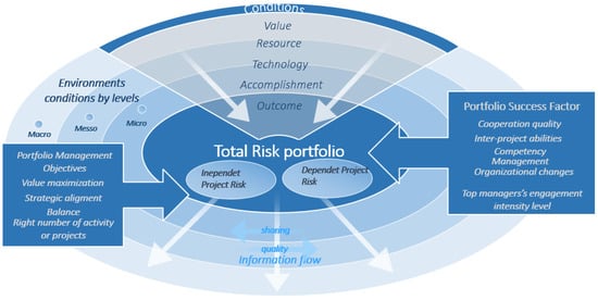
Figure 1.
Model of project risk portfolio optimization.
During the past decades, value at risk (VaR) was used as a standard tool in risk management [21] and has been used more than any other tools in this context [22]. Balbás et al. [23] found accurate approximation in VaR optimization. Artzner et al. [24] pointed out the weaknesses of value at risk, including sub-additivity, by proposing the expected shortfall measure (conditional value at risk), recommending it as the perfect risk measure, which is equal to expected loss in excess of value at risk. Another weakness of VaR is the lack of estimation for values over VaR percentage.
Relevant distribution assumptions are very important and have a great impact on estimations and quantification of risks. Slim et al. [25] shows that the normal distribution is useful only for describing the risk in low volatility state and is not satisfactory in high volatility situations. Yousefi et al. [26] examined the changes in project return based on different assumptions such as discount rate. The Monte Carlo simulation is used to investigate the effect of the changes in these factors. Tsao [27] argued that mean-VaR efficient frontier is more accurate when returns are not normal and incorporated VaR in the portfolio selection problem. The Student’s t distribution considers the fat tails of returns [28,29], and the GARCH (Generalized Autoregressive Conditionally Heteroscedastic) model efficiently captures the volatility clustering issue [30,31,32,33,34,35]. Tabasi et al. [16] used GARCH models to model the volatility-clustering feature and to estimate the parameters of the model. The Monte Carlo simulation method was used in this research for backtesting the conditional value at risk.
There have been many studies conducted on the applicability of the Conditional Extreme Value Theory (EVT), compared to other traditional methods, based on the time series and fatter tails. McNeil and Frey [36] proposed the conditional extreme value theory for the first time, by combining the extreme value theory and GARCH models. In their studies, Gençay et al. [37] and Brooks et al. [38] have compared extreme value theory with other methods of VaR estimation, such as the GARCH, and they have concluded that the extreme value theory has outperformed alternative performance models, in VaR estimation. Soltane et al. [39] have also compared the applicability of the extreme value theory in measuring value at risk and expected shortfall. The results of this study show that this method has better reaction to the changes in volatilities. By estimating value at risk via Wavelet-based EVT, Cifter [40] compared his proposed method with alternative models. Rigobon [41] and Lanne and Lütkepohl [42] used changes in the unconditional variance, while Normandin and Phaneuf [43], Lanne et al. [44], and Bouakez and Normandin [45] used conditional heteroskedasticity. Lütkepohl and Milunovich [46] and Kourouma et al. [47] focused on the forecasting strength of different methods of measuring value at risk and expected shortfall. The results of their study show that unconditional methods underestimate the risk while the extreme value theory has better estimates of risk, even during crisis. Bhattacharyya and Ritolia [48], using the conditional extreme value theory with the Peak Over Threshold model, showed that this method outperforms extreme value theory and historical simulation. Ghorbel and Trabelsi [49] evaluated the performance of different VaR measuring approaches, such as GARCH, variance-covariance, historical simulation, extreme value theory, and conditional extreme value theory. The results of this study reveal that the conditional extreme value theory, using the Peak Over Threshold model, has the best performance. Soltane et al. [39] estimated the conditional value at risk by combining GARCH and EVT models and concluded that using conditional approaches to extreme value theory improves the accuracy of the measure.
One of the advantages of the GARCH models is that consistent estimation of the model parameters does not need the knowledge of the distribution of the model errors [10]. D’Urso et al. [50], by using partitioning around medoids procedure, proposed a GARCH parametric modeling of the time series. Lütkepohl and Milunovich [46] considered GARCH models for the changes in volatility and argued about the importance of formal statistical tests for identification. Pedersen [51] considered inference in extended constant conditional correlation GARCH models and tested for volatility spillovers between foreign exchange rates. Kristjanpoller and Minutolo [52] improved volatility forecasting precision by using a hybrid model compared to the heteroscedasticity-adjusted mean squared error (HMSE) model. Sarabia et al. [53] worked with the dependent multivariate Pareto and considered a collective risk model based on dependence. Chen et al. [54] demonstrated validity of combining ST-GARCH (smooth transition-GARCH) model with Student’s t-errors and quantile forecasting for pair trading.
3. Extreme Value Models and Volatility Clustering
To properly examine the risk and return trade-off, the expectations of portfolio managers and project managers from possible risks are critical. As such, the risks of the projects are identified and estimated, and appropriate distribution is allocated according to the expectations of the managers. The aim of this research is to examine the effect of choosing various appropriate distribution on the results of this trade-off and optimization. For this, the expectations of portfolio and project managers of project risks and the distribution of projects’ returns were studied. The amount of expected risk and return in each project can be estimated based on the chosen distribution. Further, some implemented projects and their relevant risks were examined and their realized risks were compared with expected levels. Projects’ returns show fatter tails compared to normal series. This means that the chance of occurrence of extreme value returns is more than normal distribution. This finding questions the common use of normal distribution in project returns forecasting, which is quite widespread. Considering the fatter tails of returns, it can be concluded that using tail-specific models, extreme value theory, and Pareto distribution function estimates are more appropriate in estimating project risks.
As shown in Figure 2, the volatilities in historical and simulated project returns in different time periods are highly correlated. This means, based on the characteristics of each time period, the volatilities in project returns have been changed significantly. indicating a correlation in the series of returns. The existence of high and low volatilities in loss series indicates volatility clustering, which justifies the application of the GARCH model.
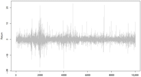
Figure 2.
Return series diagram.
In the following research, the measures of project risks are value at risk and expected shortfall. In order to estimate the parameters of these models, the following two steps must be taken:
- Estimation of assumed distribution alpha
- Estimation of return and risk forecasting models parameters
To model the value at risk and the expected shortfall, three distribution assumptions were considered: normal distribution, Student’s t-distribution (where the alpha was extracted from the relevant table), and the extended Pareto distribution, which needs the fitness of this distribution over standard errors and estimates the parameters of the distribution. In the end, the desired alpha could be calculated based on estimated parameters. In the following, the Monte Carlo method and the Hill graph were used to estimate the threshold using the R codes. It should be noted that, considering the economic conditions and the systematic changes in risks, the threshold can change, and the validity of the threshold must be tested over time. In this research, the threshold level was assumed to be fixed over the projects’ implementations.
4. Value at Risk and Expected Shortfall Models
By combining volatility forecasting models used in this study and GARCH models, and by considering two types of distribution, normal and Student’s t-distributions, four models were created. Then, by using extreme value theory for estimation of the alpha percentile, four other models were created. The unconditional extreme value model was also considered separately. Both models were examined and backtested for both measures of value at risk and expected shortfall (18 models in total).
In finance portfolio literature, numerous studies have been conducted on the estimation of value at risk and the conditional value at risk with the extreme value approach. The following proposed model of the authors is presented for project portfolio management (Table 1).

Table 1.
Value at risk (VaR) and expected shortfall models.
In this study, R [55] and MATLAB [56] were used for estimation of data and presenting diagrams for GARCH parameters’ estimation, thresholds, expected shortfall, value at risk, and backtesting of the measures.
As can be seen in Figure 3, Figure 4 and Figure 5, high and low volatilities are visible in the series for a long period of time.
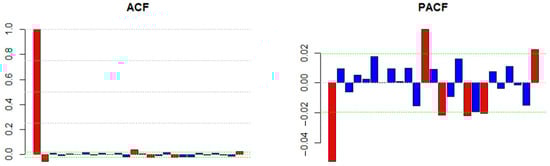
Figure 3.
Autocorrelation and partial autocorrelation of return series.
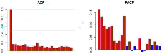
Figure 4.
Autocorrelation and partial autocorrelation of squared return series.
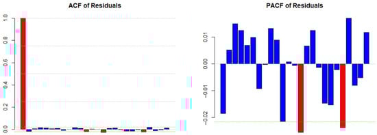
Figure 5.
Autocorrelation and partial autocorrelation of standardized residuals.
Furthermore, the existence of high and low volatilities together indicates volatility clustering, which justifies the use of the GARCH model. The autocorrelation and the partial autocorrelation diagrams are presented below. The top and the down lines show two standard deviations which indicate the confidence level of 95%.
5. Back-Testing Models
In the following table, the amount of p-value should be considered on a 5% error level. If the amount of p-value is less than the relevant level, the null hypothesis is rejected. The null hypothesis in this study was defined as if the value at risk model was estimated properly; thus, the rejection of the null hypothesis means the rejection of model validation in unconditional coverage tests, and, therefore, the higher amount of p-value means better modeling of risks.
Based on the results of Table 2, for the confidence level of 95%, none of the models were rejected, and this meant the value at risk model was appropriate. However, in the 99% confidence level, some of the models (normal distribution model) were rejected. The Student’s t-distribution models had better performance at higher confidence levels.
Table 2.
Unconditional coverage test for the value at risk models.
As can be seen in Table 2, using Peak Over Threshold models and extreme value theory in most cases improved the results.
Additionally, in Table 3 below, the use of different models did not lead to the rejection of the null hypothesis and, therefore, all the models estimated the risk properly.
Table 3.
Serial independence test for value at risk models.
As can be seen in Table 4, in higher confidence levels, the Student’s t-distribution model performed better than the normal distribution, and using extreme value theory improved the estimate of the models. In Figure 6 and Figure 7, the 99% value at risk estimation diagram for the AR(1)-GARCH(1,1) model, with the assumption of normal distribution, is given in comparison to the Peak Over Threshold model.
Table 4.
Conditional coverage test for value at risk models.
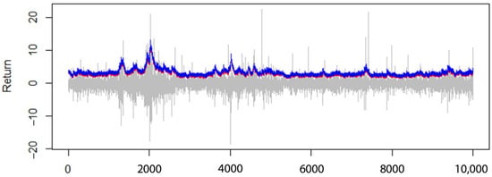
Figure 6.
The 95% VaR (VaR0.95) for AR(1)-GARCH(1,1) model, with normal distribution assumption (red line) compared to the Peak Over Threshold model (blue line).
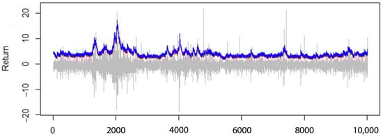
Figure 7.
The 99% VaR (VaR0.99) for AR(1)-GARCH(1,1) model, with normal distribution assumption (red line) compared to the Peak Over Threshold model (blue line).
It can be expected that we can reach similar results with value at risk models for the validity of the expected shortfall models. However, the rank of desirability of these models may vary.
The V test was used to examine the performance of expected shortfall models [46]. In ref [28], the validity is examined, but in ref [46] model, the performance of the models can be compared with each other as well.
In the V1 test, the performance of expected shortfall models (similar to ref [28]) was dependent on the validity of the value at risk model.
In the V2 test, the backtesting of the expected shortfall model was performed independently from the validity of the value at risk model.
The V model could be calculated by summing up the absolute value of V1 and V2 statistics; the closer the value was to zero, the more credible was the model.
As can be seen in Table 5, the zero hypothesis with the assumption of the normal distribution was rejected in most of the expected shortfall models. This indicates the fact that the normal distribution assumption for the estimation of expected shortfall models was not valid. This is consistent with the results of the ref [36] study. Furthermore, it can be seen that using extreme value theory improved the models. According to the results presented in Table 5, the Student’s t-distribution model had better performance in comparison to the normal models. The usage of Peak Over Threshold estimation in expected shortfall models, with the assumption of the Student’s t-distribution, led to a decrease in the p-value. However, in most cases, the null hypothesis was not rejected. It can be concluded that using the Student’s t-distribution assumption in expected shortfall models lead to an overestimation of risk. This overestimation of risk can be adjusted using Peak Over Threshold models.
Table 5.
The bootstrap test for the expected shortfall models.
In Table 6, the results of the V1 test is presented. The closer these numbers were to zero, the higher was the validity of the model. Using this table, we can see the overestimation or the underestimation of the models. The values of the normal distribution models were positive and had larger numerical values, which indicates the underestimation of risks. The Student’s t-distribution models, in some cases, led to negative estimations and, therefore, overestimation of risks. Generally, the Peak Over Threshold models and the Pareto distribution improved the models.
Table 6.
The V1 test for the expected shortfall models.
According to the studies conducted by Embrechts et al. [57], the backtesting of the expected shortfall model can be done via the V2 test, independent of value at risk models. According to the results presented in Table 7, using the normal distribution led to underestimation of risks. Table 8 shows the V test for the expected shortfall models
Table 7.
The V2 test for the expected shortfall models.
Table 8.
The V test for the expected shortfall models.
Finally, the V model could also be calculated by averaging the absolute values of V1 and V2, and the closer the value was to zero, the more valid was the model. In Figure 8, the 95% expected shortfall estimation diagram for AR(1)-GARCH(1,1) model, and in Figure 9, the 99% expected shortfall estimation diagram for AR(1)-GARCH(1,1) model, with the assumption of normal distribution, are given in comparison to the Peak Over Threshold model.
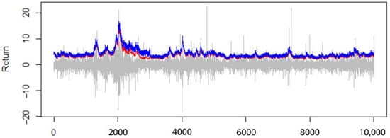
Figure 8.
The 95% expected shortfall (ES0.95) for AR(1)-GARCH(1,1) model, with normal distribution assumption (red line) compared to the Peak Over Threshold model (blue line).
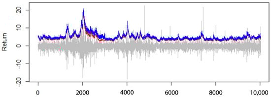
Figure 9.
The 99% expected shortfall (ES0.99) for AR(1)-GARCH(1,1) model, with normal distribution assumption (red line) compared to the Peak Over Threshold model (blue line).
6. Conclusions
Based on the studies, it can be concluded that the risks of the studied construction projects, in addition to skewness, have higher kurtosis and fatter tails in comparison to the normal distribution. Therefore, the assumption of normal distribution is not suitable for estimation of risk and leads to the underestimation of risk, especially in higher confidence levels. Assumption of Student’s t-distribution has better performance in risk estimation measures. Even though the Student’s t-distribution assumption in some cases led to the overestimation of risks, because of its conservative approach, it is more appropriate than the normal distribution. The differences between these models are more intelligible in higher confidence levels. The application of the extreme value theory in most cases led to the superior performance of the models and adjusted the underestimations of the normal distribution and the overestimations of the Student’s t-distribution. The changes in the returns of the studied projects indicate the volatility clustering, and, therefore, the application of GARCH models for modeling these characteristics can be confirmed.
Therefore, because of the importance of proper estimation of risks, it is recommended not to use the normal distribution in risk and return optimization problems for choosing the appropriate projects. The proposition of this study is the use of Student’s t-distribution assumption combined with extreme value theory and using the GARCH models because of the volatility clustering.
Author Contributions
V.Y. designed the research, set the objectives, studied the literature, analyzed data, designed and developed the model. V.Y., J.T., and H.T. gathered and analyzed the data, revised the manuscript, methodology and findings, and provided extensive advice on the literature review, model development and its evaluation. Conceptualization, V.Y.; methodology, V.Y. and H.T.; software, V.Y. and H.T.; validation, formal analysis, investigation, resources, data curation, writing—original draft preparation, V.Y., J.T., and H.T.; writing—review and editing, J.T. and H.T.; visualization, V.Y., J.T., and H.T.; supervision, J.T.; project administration, V.Y., J.T., and H.T. All authors discussed the model evaluation results and commented on the paper. All authors have read and agreed to the published version of the manuscript.
Funding
This research received no external funding.
Institutional Review Board Statement
Not applicable.
Informed Consent Statement
Not applicable.
Data Availability Statement
Data available on request due to restrictions.
Conflicts of Interest
The authors declare no conflict of interest.
References
- Vacik, E.; Špaček, M.; Fotr, J.; Kracík, L. Project portfolio optimization as a part of strategy implementation process in small and medium-sized enterprises: A methodology of the selection of projects with the aim to balance strategy, risk and performance. Econ. Manag. 2018, 21, 107–123. [Google Scholar]
- Shi, Q.; Liu, Y.; Zuo, J.; Pan, N.; Ma, G. On the management of social risks of hydraulic infrastructure projects in China: A case study. Int. J. Proj. Manag. 2015, 33, 483–496. [Google Scholar] [CrossRef]
- Becker, K.; Smidt, M. Workforce-related risks in projects with a contingent workforce. Int. J. Proj. Manag. 2015, 33, 889–900. [Google Scholar] [CrossRef]
- Thomé, A.M.T.; Scavarda, L.F.; Scavarda, A.; de Souza Thomé, F.E.S. Similarities and contrasts of complexity, uncertainty, risks, and resilience in supply chains and temporary multi-organization projects. Int. J. Proj. Manag. 2016, 34, 1328–1346. [Google Scholar] [CrossRef]
- Qazi, A.; Quigley, J.; Dickson, A.; Kirytopoulos, K. Project Complexity and Risk Management (ProCRiM): Towards modelling project complexity driven risk paths in construction projects. Int. J. Proj. Manag. 2016, 34, 1183–1198. [Google Scholar] [CrossRef]
- Yang, R.J.; Zou, P.X.W.; Wang, J. Modelling stakeholder-associated risk networks in green building projects. Int. J. Proj. Manag. 2016, 34, 66–81. [Google Scholar] [CrossRef]
- Pfeifer, J.; Barker, K.; Ramirez-Marquez, J.E.; Morshedlou, N. Quantifying the risk of project delays with a genetic algorithm. Int. J. Prod. Econ. 2015, 170, 34–44. [Google Scholar] [CrossRef]
- Liu, J.; Jin, F.; Xie, Q.; Skitmore, M. Improving risk assessment in financial feasibility of international engineering projects: A risk driver perspective. Int. J. Proj. Manag. 2017, 35, 204–211. [Google Scholar] [CrossRef]
- Yousefi, V.; Yakhchali, S.H.; Šaparauskas, J.; Kiani, S. The Impact Made on Project Portfolio Optimisation by the Selection of Various Risk Measures. Eng. Econ. 2018, 29, 168–175. [Google Scholar] [CrossRef]
- Namazian, A.; Yakhchali, S.H.; Yousefi, V.; Tamošaitienė, J. Combining Monte Carlo Simulation and Bayesian Networks Methods for Assessing Completion Time of Projects under Risk. Int. J. Environ. Res. Public Health 2019, 16, 5024. [Google Scholar] [CrossRef]
- Sarvari, H.; Rakhshanifar, M.; Tamošaitienė, J.; Chan, D.W.M.; Beer, M. A Risk Based Approach to Evaluating the Impacts of Zayanderood Drought on Sustainable Development Indicators of Riverside Urban in Isfahan-Iran. Sustainability 2019, 11, 6797. [Google Scholar] [CrossRef]
- Hatefi, S.M.; Tamosaitiene, J. Construction Projects Assessment Based on the Sustainable Development Criteria by an Integrated Fuzzy AHP and Improved GRA Model. Sustainability 2018, 10, 991. [Google Scholar] [CrossRef]
- Hatefi, S.M.; Basiri, M.E.; Tamosaitiene, J. An Evidential Model for Environmental Risk Assessment in Projects Using Dempster-Shafer Theory of Evidence. Sustainability 2019, 11, 6329. [Google Scholar] [CrossRef]
- Shrestha, A.; Tamosaitiene, J.; Martek, I.; Hosseini, M.R.; Edwards, D.J. A Principal-Agent Theory Perspective on PPP Risk Allocation. Sustainability 2019, 11, 6455. [Google Scholar] [CrossRef]
- Valipour, A.; Yahaya, N.; Md Noor, N.; Valipour, I.; Tamosaitiene, J. A SWARA-COPRAS approach to the allocation of risk in water and sewerage Public-Private Partnership Projects in Malaysia. Int. J. Strateg. Prop. Manag. 2019, 23, 269–283. [Google Scholar] [CrossRef]
- Tabasi, H.; Yousefi, V.; Tamosaitiene, J.; Ghasemi, F. Estimating Conditional value at risk in the Tehran Stock Exchange Based on the Extreme Value Theory Using GARCH Models. Adm. Sci. 2019, 9, 40. [Google Scholar] [CrossRef]
- Dixit, V.; Tiwari, M.K. Project portfolio selection and scheduling optimization based on risk measure: A conditional value at risk approach. Ann. Oper. Res. 2020, 285, 9–33. [Google Scholar] [CrossRef]
- Hatefi, S.M.; Tamosaitiene, J. An Integrated Fuzzy Dematel-Fuzzy ANP Model for Evaluating Construction Projects by Considering Interrelationships among Risk Factors. J. Civ. Eng. Manag. 2019, 25, 114–131. [Google Scholar] [CrossRef]
- Ghasemi, F.; Sari, M.H.M.; Yousefi, V.; Falsafi, R.; Tamosaitiene, J. Project Portfolio Risk Identification and Analysis, Considering Project Risk Interactions and Using Bayesian Networks. Sustainability 2018, 10, 1609. [Google Scholar] [CrossRef]
- Ahmadi-Javid, A.; Fateminia, S.H.; Gemünden, H.G. A Method for Risk Response Planning in Project Portfolio Management. J. Proj. Manag. 2020, 51, 77–95. [Google Scholar] [CrossRef]
- Spierdijk, L. Confidence intervals for ARMA–GARCH Value-at-Risk: The case of heavy tails and skewness. Comput. Stat. Data Anal. 2016, 100, 545–559. [Google Scholar] [CrossRef]
- Micán, C.; Fernandes, G.; Araújo, M. Project portfolio risk management: A structured literature review with future directions for research. Int. J. Inf. Syst. Proj. Manag. 2020, 8, 67–84. [Google Scholar]
- Balbás, A.; Balbás, B.; Balbás, R. VaR as the CVaR sensitivity: Applications in risk optimization. J. Comput. Appl. Math. 2017, 309, 175–185. [Google Scholar] [CrossRef]
- Artzner, P.; Delbaen, F.; Eber, J.M.; Heath, D. Coherent measures of risk. Math. Financ. 1999, 9, 203–228. [Google Scholar] [CrossRef]
- Slim, S.; Koubaa, Y.; BenSaïda, A. Value-at-Risk under Lévy GARCH models: Evidence from global stock markets. J. Int. Financ. Mark. I 2017, 45, 30–53. [Google Scholar] [CrossRef]
- Yousefi, V.; Yakhchali, S.H.; Tamošaitienė, J. Application of Duration Measure in Quantifying the Sensitivity of Project Returns to Changes in Discount Rates. Admin. Sci. 2019, 9, 13. [Google Scholar] [CrossRef]
- Tsao, C.Y. Portfolio selection based on the mean–VaR efficient frontier. Quant. Financ. 2010, 10, 931–945. [Google Scholar] [CrossRef]
- Christoffersen, P.F. Elements of Financial Risk Management; Academic Press: Cambridge, MA, USA, 2012. [Google Scholar]
- Huisman, R.; Koedijk, K.G.; Pownall, R.A. VaR-x: Fat tails in financial risk management. J. Risk 1998, 1, 47–61. [Google Scholar] [CrossRef]
- Alexander, C.; Sheedy, E. Developing a stress testing framework based on market risk models. J. Bank. Financ. 2008, 32, 2220–2236. [Google Scholar] [CrossRef]
- Alexander, C. Market Risk Analysis, value at risk Models; John Wiley and Sons: Hoboken, NJ, USA, 2009; Volume 4. [Google Scholar]
- Berkowitz, J.; O’brien, J. How accurate are value-at-risk models at commercial banks? J. Financ. 2002, 57, 1093–1111. [Google Scholar] [CrossRef]
- Hull, J.; White, A. Incorporating volatility updating into the historical simulation method for value-at-risk. J. Risk 1998, 1, 5–19. [Google Scholar] [CrossRef]
- Pritsker, M. The hidden dangers of historical simulation. J. Bank. Financ. 2006, 30, 561–582. [Google Scholar] [CrossRef]
- Ranković, V.; Drenovak, M.; Urosevic, B.; Jelic, R. Mean-univariate GARCH VaR portfolio optimization: Actual portfolio approach. Comput. Oper. Res. 2016, 72, 83–92. [Google Scholar] [CrossRef]
- McNeil, A.J.; Frey, R. Estimation of tail-related risk measures for heteroscedastic financial time series: An extreme value approach. J. Empir. Financ. 2000, 7, 271–300. [Google Scholar] [CrossRef]
- Gençay, R.; Selçuk, F.; Ulugülyaǧci, A. High volatility, thick tails and extreme value theory in value-at-risk estimation. Insur. Math. Econ. 2003, 33, 337–356. [Google Scholar] [CrossRef]
- Brooks, C.; Clare, A.D.; Dalle Molle, J.W.; Persand, G. A comparison of extreme value theory approaches for determining value at risk. J. Empir. Financ. 2005, 12, 339–352. [Google Scholar] [CrossRef]
- Soltane, H.B.; Karaa, A.; Bellalah, M. Conditional VaR Using GARCH-EVT Approach: Forecasting Volatility in Tunisian Financial Market. J. Comput. Model. 2012, 2, 95–115. [Google Scholar]
- Cifter, A. Value-at-risk estimation with wavelet-based extreme value theory: Evidence from emerging markets. Phys. A 2011, 390, 2356–2367. [Google Scholar] [CrossRef]
- Rigobon, R. Identification through Heteroskedasticity. Rev. Econ. Stat. 2003, 85, 777–792. [Google Scholar] [CrossRef]
- Lanne, M.; Lütkepohl, H. Identifying Monetary Policy Shocks via Changes in Volatility. J. Money Credit Bank. 2008, 40, 1131–1149. [Google Scholar] [CrossRef]
- Normandin, M.; Phaneuf, L. Monetary policy shocks: Testing identification conditions under time-varying conditional volatility. J. Monet. Econ. 2004, 51, 1217–1243. [Google Scholar] [CrossRef]
- Lanne, M.; Lütkepohl, H.; Maciejowska, K. Structural vector autoregressions with Markov switching. J. Econ. Dyn. Control 2010, 34, 121–131. [Google Scholar] [CrossRef]
- Bouakez, H.; Normandin, M. Fluctuations in the foreign exchange market: How important are monetary policy shocks? J. Int. Econ. 2010, 81, 139–153. [Google Scholar] [CrossRef]
- Lütkepohl, H.; Milunovich, G. Testing for identification in SVAR-GARCH models. J. Econ. Dyn. Control 2016, 73, 241–258. [Google Scholar] [CrossRef]
- Kourouma, L.; Dupre, D.; Sanfilippo, G.; Taramasco, O. Extreme value at risk and expected shortfall during financial crisis. SSRN 2010. [Google Scholar] [CrossRef]
- Bhattacharyya, M.; Ritolia, G. Conditional VaR using EVT–Towards a planned margin scheme. Int. Rev. Financ. Anal. 2008, 17, 382–395. [Google Scholar] [CrossRef]
- Ghorbel, A.; Trabelsi, A. Predictive performance of conditional extreme value theory in value-at-risk estimation. Int. J. Monet. Econ. Financ. 2008, 1, 121–148. [Google Scholar] [CrossRef]
- D’Urso, P.; De Giovanni, L.; Massari, R. GARCH-based robust clustering of time series. Fuzzy Set. Syst. 2016, 305, 1–28. [Google Scholar] [CrossRef]
- Pedersen, R.S. Inference and testing on the boundary in extended constant conditional correlation GARCH models. J. Econom. 2017, 196, 23–36. [Google Scholar] [CrossRef][Green Version]
- Kristjanpoller, W.; Minutolo, M.C. Forecasting volatility of oil price using an artificial neural network-GARCH model. Expert Syst. Appl. 2016, 65, 233–241. [Google Scholar] [CrossRef]
- Sarabia, J.M.; Gómez-Déniz, E.; Prieto, F.; Jordá, V. Risk aggregation in multivariate dependent Pareto distributions. Insur. Math. Econ. 2016, 71, 154–163. [Google Scholar] [CrossRef]
- Chen, C.W.S.; Wang, Z.; Sriboonchitta, S.; Lee, S. Pair trading based on quantile forecasting of smooth transition GARCH models. N. Am. J. Econ. Financ. 2017, 39, 38–55. [Google Scholar] [CrossRef]
- R Core Team. R: A Language and Environment for Statistical Computing; R Foundation for Statistical Computing: Vienna, Austria, 2020; Available online: https://www.R-project.org/.
- The Math Works, Inc. MATLAB; Version 2020a; The Math Works, Inc.: Natick, MA, USA, 2020; Computer Software. [Google Scholar]
- Embrechts, P.; Kaufmann, R.; Patie, P. Strategic long-term financial risks: Single risk factors. Comput. Optim. Appl. 2005, 32, 61–90. [Google Scholar] [CrossRef]


Publisher’s Note: MDPI stays neutral with regard to jurisdictional claims in published maps and institutional affiliations. |
© 2021 by the authors. Licensee MDPI, Basel, Switzerland. This article is an open access article distributed under the terms and conditions of the Creative Commons Attribution (CC BY) license (http://creativecommons.org/licenses/by/4.0/).