Solar Photovoltaic Power Prediction Using Big Data Tools

Abstract

Solar photovoltaic (PV) installation has been continually growing to be utilized in a grid-connected or stand-alone network. However, since the generation of solar PV power is highly variable because of different factors, its accurate forecasting is critical for a reliable integration to the grid and for supplying the load in a stand-alone network. This paper presents a prediction model for calculating solar PV power based on historical data, such as solar PV data, solar irradiance, and weather data, which are stored, managed, and processed using big data tools. The considered variables in calculating the solar PV power include solar irradiance, efficiency of the PV system, and characteristics of the PV system. The solar PV power profiles for each day of January, which is a summer season, were presented to show the variability of the solar PV power in numerical examples. The simulation results show relatively accurate forecasting with 17.57 kW and 2.80% as the best root mean square error and mean relative error, respectively. Thus, the proposed solar PV power prediction model can help power system engineers in generation planning for a grid-connected or stand-alone solar PV system.

1. Introduction

The utilization and the development of renewable energy sources (i.e., solar, wind, hydropower, biomass power, geothermal, and concentrated solar power (CSP)) have been one of the solutions to the depletion of fossil fuel used in conventional power sources and to the reduction of pollution. In addition, renewable energy sources are also used to provide power to the grid and the stand-alone network. From the additional power capacities from renewable energy sources in 2016, the highest additional capacity is from solar photovoltaic (PV) which accounts for 47%, whereas 34% is from wind, 15.5% is from hydropower, and 3.5% is from other renewable energy sources (i.e., biomass power, geothermal power, and CSP) [1]. These additional power capacities came from the top ten markets which include China, the United States, Japan, India, the United Kingdom, Germany, the Republic of Korea, Australia, the Philippines, and Chile [1]. According to the Australian Renewable Energy Agency (ARENA), Australia has the highest solar radiation per square meter, which is considered to have some of the best solar energy sources in the world [2]. Hence, the additional capacity from solar PV power in Australia is nearly 0.9 GW which is from the combined development of small, medium, and large-scale solar technologies [1]. Therefore, the integration of solar PV power to the grid and stand-alone network has been studied and developed. However, since solar energy sources are intermittent, as it depends on the amount of sunlight at a given time in a particular place, they cause problems in balancing the supply and demand. To closely match the fluctuating solar PV power generation to the demand, an accurate prediction of solar PV power is necessary. A reliable prediction result will help determine whether there is a shortage or excess in solar PV power generation. Therefore, different prediction methods have been developed and used to predict solar PV power. These methods are classified into three major methods that include time series methods, physical methods, and hybrid methods [3].

Time-series methods are highly dependent on historical data, which consist of a sequence of observations over time. The relationship between the historical data was constructed to be used in modeling the prediction model in this method. These time series methods include autoregressive [4,5,6,7], artificial neural network (ANN) [8,9,10,11], support vector machine (SVM) [12,13], and Markov chain [14,15]. Different autoregressive models are used in forecasting solar PV power, such as autoregressive moving average (ARMA) which is applied to stationary time series [4,5], autoregressive integrated moving average (ARIMA) which deals with nonstationary time series [5,6], and autoregressive moving average with exogenous inputs (ARMAX) which considers the external factors influencing the variable to be forecasted [7]. Study [4] applied the ARMA model and the persistence model to predict solar generation using historical solar radiation data, whereas study [5] compared ARMA and ARIMA models for multi-periods, one-period, two-periods, and three-periods ahead for prediction of solar radiation. In a study [6], a comparison of different methods for forecasting solar radiation was evaluated using ARIMA, Unobserved Components models, transfer function, neural networks, and hybrid models. Whereas the ARMAX model was suggested by study [7] to consider the exogenous inputs to forecast the power output of a grid-connected PV system. These previous studies that used time series methods [4,5,6,7] required a large amount of historical data. To handle this large amount of historical data efficiently, this paper proposed a solar PV power prediction model using big data tools.

Meanwhile, ANN is a mathematical model which is developed based on the operation of the biological neural system. ANN has been used in many applications in solving complex nonlinear data and pattern recognition where its accuracy depends on input parameters, training algorithm, and structure configuration [3]. The typical ANN structure consists of the input layer, hidden layer, and output layer [3]. In a previous study [8], the mean daily solar irradiance and air temperature were used as input variables to ANN models which used a Multilayer Perceptron model to forecast the output of 24 h solar irradiance. In a study [9], the time horizon with the highest representative for generated solar power prediction of the small-scale solar power system was determined. Meanwhile, study [10] used two ANN models which considered the power of the PV plant and radiation as the inputs to forecast the output power of the PV power plant. Moreover, two neural network structures, such as the general regression neural network and backpropagation, were used to model the PV panel output power which used temperature and irradiance as inputs in a study [11]. Compared with these previous studies [8,9,10,11] which use solar irradiance and temperature as data, this paper uses other weather data such as humidity, wind speed, precipitation, cloudiness, and weather condition, in addition to solar irradiance and temperature. In addition, SVM is a machine-learning technique used in forecasting solar PV power. It has also been used in pattern recognition, object classification, and regression analysis [16]. In a previous study [12], one-day-ahead PV power output was predicted based on weather data and power output data using SVM. In study [13], the historical data of transmissivity and the meteorological parameters were used in forecasting solar power using least-square SVM. Moreover, the Markov chain is also one of the time series methods which is a stochastic process in which a probability of a certain state depends on one or more previous states. In a previous study [14], the PV system was divided into several states considering the weather condition, solar radiation, and other factors which are calculated by the Markov chain mathematical model to forecast generation capacity. Compared to these previous studies [8,9,10,11,12,13,14,15] that used complex structure configuration, this paper provides a simple and straightforward solar power prediction model.

Second, physical methods are another major method in forecasting solar PV power. They are used when the atmospheric components are available to determine their effect on solar radiations. To measure these components, an appropriate device is necessary. Different tools were used, such as numerical weather prediction [17], sky imagery [18], and satellite imaging [19]. Furthermore, with the limitations of the individual methods discussed above, the use of hybrid methods [20,21,22,23] was presented to enhance the strengths and to improve the forecasting performance of the individual methods. As stated above, different techniques and methods were used in forecasting solar PV power; however, big data tools have not been used in forecasting solar PV power. Therefore, this paper proposes a solar PV power prediction model that uses big data tools based on solar PV power data, solar irradiance data, and weather data.

In this paper, the technical architecture using big data technologies presented in the previous study [24] is the basis of the methods used in formulating the proposed solar PV power prediction model. Study [24] applied this technical architecture in forecasting EV charging demand, and this is applied in formulating the solar PV power prediction model in this paper. Since this is applied to different data, different approaches and calculations were used in this paper compared to the previous study [24]. In this paper, the proposed methods for the solar PV power prediction model include storing historical data, managing historical data, and processing historical data. These historical data include the solar PV power data, solar irradiance data, and weather data of the University of Queensland, Australia. In storing and managing historical data, the big data tools that include built-in functions in MATLAB are used in this paper. In processing the historical data, three approaches are used, including clustering solar irradiance patterns, identifying significant factors affecting solar irradiance, and forming a decision tree. Once the solar irradiance cluster is determined based on the forecast weather data using the decision tree, the solar PV power is calculated using the solar irradiance, the efficiency of the PV system, and the characteristics of the PV system (i.e., area of the PV module of the PV system).

As another technique and method in accurately predicting solar PV power, the contributions of this paper are the following:

• This paper introduces the use of big data tools in forecasting solar PV power. With different methods and techniques presented in forecasting solar PV power in previous studies [4,5,6,7,8,9,10,11,12,13,14,15,16,17,18,19,20,21,22,23], big data tools have not been applied in forecasting solar PV power. This paper develops the solar PV power prediction model using big data tools based on actual data. Since time series methods [4,5,6,7,8,9,10,11,12,13,14,15] are highly dependent on historical data that consists of a sequence of data, a larger amount of historical data is necessary for the formulation of the forecasting model to procure an accurate result using these methods. However, processing this large amount of data requires a lot of time and computer memory. The use of big data tools may address these issues and challenges in processing a large amount of data, and thus provide an efficient prediction of solar PV power. In addition, the formulation of a solar PV power prediction model using big data tools is simple and straightforward compared to modeling a solar PV power prediction model using time series methods.
• In addition, this paper considers other weather data such as humidity, wind speed, precipitation, cloudiness, and weather condition, in addition to temperature, in formulating the solar PV power prediction model. Compared to previous studies [8,9,11] that use temperature and solar irradiance as input variables for forecasting solar irradiance or solar PV power, this paper considers solar irradiance, average temperature, average humidity, average wind speed, average precipitation, cloudiness, and weather condition in formulating a solar PV power prediction model. These weather data (i.e., solar irradiance, average temperature, average humidity, average wind speed, average precipitation, cloudiness, and weather condition) are the factors that influence the calculated solar PV power. In this paper, the factors that significantly affect solar irradiance are identified.
• Furthermore, based on the simulation results of this paper, the forecasting performance was improved using the proposed solar PV power prediction model. Different forecasting error measurements were used in previous studies [4,5,6,7,8,9,10,11,12,13,14,15,17,18,19,20,21,22,23] to verify the performance of the forecasting model. In this paper, the root mean square error (RMSE) and the mean relative error (MRE) were used to verify the effectiveness of the proposed solar PV power prediction model. Compared with previous studies [12,22] that use RMSE and MRE as the evaluation indices, this paper shows a relatively lower MRE result. Considering the lower error, the proposed solar PV power prediction model can provide a relatively accurate forecasting result in determining if there is a shortage or excess of solar PV power generation that will be used to supply the grid or the load in a stand-alone network. Using these results, the proposed solar PV power prediction model can help provide reliable power to these networks.

The remainder of this paper is organized as follows: the materials and methods used in formulating the solar PV power prediction model using big data tools are described in Section 2. A numerical example presenting the results that include the solar PV power profiles of the whole month of a summer season is presented in Section 3 to illustrate the effectiveness of the proposed solar PV power prediction model. Finally, Section 4 discusses the results of the paper with a summary of findings.

2. Materials and Methods

This paper develops a solar PV power prediction model using big data tools utilized in a previous study [24]. In the previous study [24], the technical architecture based on big data tools used in the EV charging demand forecasting model has four layers that include data sources, data storage, data management, and data processing. In this paper, the methodology used in formulating a solar PV power prediction model includes storing historical data, managing historical data, processing historical data, and solar PV power calculation shown in Figure 1.

The historical data used in this paper include solar PV data, solar irradiance data, and weather data in Australia. The solar PV data and the solar irradiance data were collected every minute from 1 January 2012 to 31 January 2017 in the University of Queensland (UQ), Australia [25]. These historical solar PV data and solar irradiance data were collected from the UQ PV site specifically from the UQ Centre of the St. Lucia campus with a capacity of 433.44 kW and a PV module area of 2956 m², which uses a polycrystalline silicon type of solar cells. The historical solar PV data includes power and energy which were collected from 5:00 to 18:59 whereas the historical solar irradiance data were collected from 0:00 to 23:59. The historical weather data, which include temperature, feels, humidity, wind speed, gust, pressure, precipitation, chance of precipitation, cloudiness, visibility, and weather condition, were collected every hour [26]. In this paper, the historical data collected from 1 January 2012 to 31 January 2016 were considered as the training data whereas the historical data collected from the whole month of January 2017 were considered as the testing data.

2.1. Storing Historical Data

Storing historical data is the first method used in formulating the solar PV power prediction model in which the historical data from 1 January 2012 to 31 January 2017 were stored in a local disk on a computer. From these stored historical data, the necessary data for the formulation of the solar PV power prediction model was accessed. This paper used the Datastore function in MATLAB to access the necessary data which include the historical solar PV power, historical solar irradiance, and historical weather data (i.e., temperature, humidity, wind speed, precipitation, cloudiness, and weather condition). This function provides these necessary data in a chunk-like manner to have a faster and more effective way of accessing these historical data. The output of this method is the necessary historical data used in the formulation of the solar PV power prediction model which includes solar PV power, solar irradiance, and weather data (i.e., temperature, humidity, wind speed, precipitation, cloudiness, and weather condition).

2.2. Managing Historical Data

The second method used in formulating the solar PV power prediction model is managing the necessary historical data (i.e., solar PV power, solar irradiance, weather data) accessed from the previous method. As stated above, the historical solar PV power was collected every minute from 5:00 to 18:59, the historical solar irradiance data were also collected every minute from 0:00 to 23:59, whereas the historical weather data were collected every hour from 0:00 to 23:00. To organize the historical data to have the same time range, the MapReduce function in MATLAB was used to access only the historical solar irradiance from 5:00 to 18:59. This will provide all the necessary historical data for the formulation of a solar PV power prediction model in a uniform structure. In addition, to avoid high errors due to missing data, these missing values were filled with the values of the previous minute. Lastly, these necessary historical data were grouped according to a month to consider the effect of monthly weather data on solar irradiance. Figure 2 shows all the historical solar irradiance data of the month of January collected every minute from 5:00 to 18:59 for five years (i.e., 2012 to 2016). Each color in Figure 2 represents one day in the month of January from 2012 to 2016. All these historical solar irradiances have a mean solar irradiance of 460 W/m² which is represented by the line. The month of January was chosen to show the solar PV power profile of the summer season in Australia. The summer season was chosen because solar irradiance is highest during this season.

2.3. Processing Historical Data

Processing historical data is the third method in formulating the solar PV power prediction model as shown in Figure 1. In this paper, the approaches used for processing the historical data includes clustering the solar irradiance pattern, identifying significant factors affecting solar irradiance, and forming a decision tree.

2.3.1. Clustering Solar Irradiance Pattern

In this approach, the historical solar irradiance pattern for the month of January from 2012 to 2015 shown in Figure 2 was classified into clusters based on their similarities. In this paper, agglomerative hierarchical clustering was used to group solar irradiance data in a multilevel hierarchy. The first level is to find the similarity between each datum of the solar irradiance. Then, these objects are paired into a group that form a larger group until a hierarchical tree is formed. Lastly, the hierarchical tree is cut into clusters. In this paper, three built-in functions (i.e., Pdist, Linkage, and Cluster) in MATLAB were used in each level to cluster the historical solar irradiance.

In the first level, the Pdist function was used to calculate distance based on the similarity between every datum of solar irradiance. To determine their similarities, this function computes the Euclidean distance between two data points. Given a matrix with m (1 × n) and row vectors x₁, x₂, …, x_m, the distance between the vector x_i and x_j is calculated as [24,27]:

$$d_{ij}=\sqrt{{\sum }_{k=1}^n{\left(x_{ik}-x_{jk}\right)}^2},$$

(1)

Next, the calculated distance from the Pdist function was used by the Linkage function to group the data into a multilevel hierarchical tree. In this function, the distance between two groups is calculated to determine the proximity of data to each other. In this paper, the smallest distance between the data in the two groups was used, which is given as [27]:

$$\begin{array}{cc}{d}_{rs}=min\left[dist\left(x_{ri},x_{sj}\right)\right]& i\in \left(1,\dots ,n_r\right)\\ & j\in \left(1,\dots ,n_s\right)\end{array},$$

(2)

where n_r and n_s are the numbers of data in group r and s, respectively, and x_ri and x_sj are the ith and jth data in group r and s, respectively. As the data are paired into groups, larger groups are formed into a hierarchical tree.

Lastly, the Cluster function was used to determine the partition to form clusters by detecting natural groupings in the hierarchical tree or by cutting off the hierarchical tree arbitrarily. This function provides clusters from an agglomerative hierarchical cluster tree formed using the output of the Linkage function. Since hierarchical clustering requires a number of clusters, the silhouette evaluation index was used to determine the number of clusters to be input when cutting off the hierarchical tree into clusters. The silhouette method determines the similarity between the object and the cluster. The silhouette evaluation index has a range of –1 to 1, in which a silhouette evaluation index close to 1 indicates a close relationship between the object and the cluster. The Evalclusters’ built-in function in MATLAB was used to create a criterion in clustering which calculated the silhouette evaluation index as [27]:

$$s_i=\frac{\left(b_i-a_i\right)}{max\left(a_i,b_i\right)},$$

(3)

where a_i is the average distance from the ith point to the other points in the same cluster as i, and b_i is the minimum average distance from the ith point to the points in a different cluster.

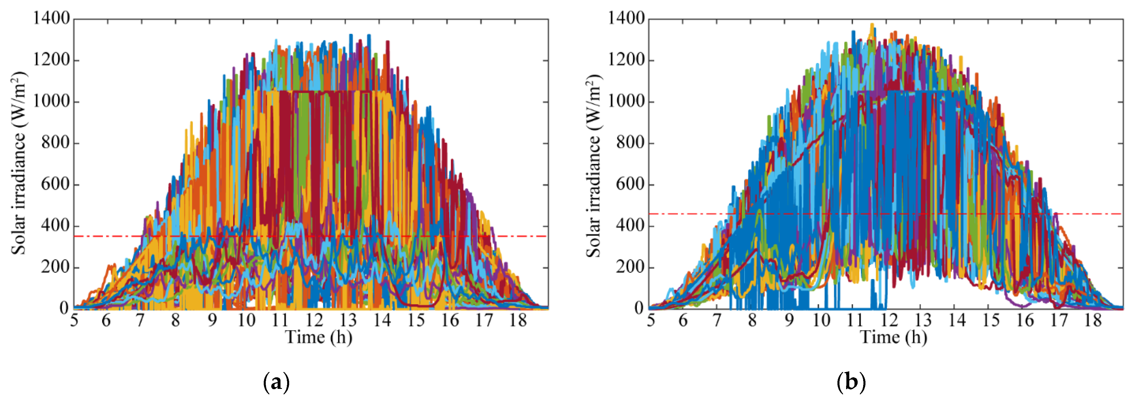
As a result, there are two optimal numbers of clusters classified, as shown in Figure 3. Figure 3 shows the clustered historical solar irradiance data. Since there are two clusters classified using the silhouette method, the historical solar irradiance data in Figure 2 is divided into two clusters using agglomerative hierarchical clustering. Figure 3a shows the first cluster of the solar irradiance classified from Figure 2. As observed in Figure 3a, the solar irradiance pattern includes the days with lower solar irradiance which were affected by external factors, such as clouds. Figure 3b shows the second cluster of solar irradiance patterns classified from Figure 2. These solar irradiance patterns include higher solar irradiance throughout the considered time range (i.e., 5:00 to 18:59). As shown in Figure 3, the solar irradiance patterns in cluster 1 and cluster 2 have mean solar irradiances of 352.4 W/m² and 460 W/m², respectively. These calculated means indicate that the solar irradiance in cluster 1 is lower compared to that in cluster 2.

2.3.2. Identifying Significant Factors Affecting Solar Irradiance

Solar irradiance is affected by many factors, such as the weather. Most of the studies [8,9,11] consider only the effect of temperature in solar irradiance. In this paper, the effect of other weather data, such as humidity, wind speed, precipitation, cloudiness, and weather condition, on solar irradiance were also considered. Humidity affects the reception of solar which reduces the amount of received solar radiation of the PV module [28]. In addition, a study [29] provided the statistical relationship between solar radiation, sunshine, and relative humidity of the environment to provide reasonable estimates of solar radiation in areas where no other data is available. The previous study estimated solar radiation as [29]:

Q = 464 + 265S − 248R,

(4)

where Q is the solar radiation in Watt-hour/m², S is the ratio of the recorded hours of bright sunshine to a fixed reference of 12 h, and R is the relative humidity as a percent. From (4), solar radiation was estimated using humidity which assumes that humidity affects solar radiation. Hence, humidity is another factor that affects solar irradiance in this paper.

In addition, wind speed may also affect the solar reception of the PV module because it helps assist reduce the dirt on the surface of the PV module to a certain extent [30]. Moreover, precipitation (i.e., rain) may also affect solar irradiance as rain helps in washing and removing dirt on the surface of the PV module. A previous study [31] developed a model and analysis of PV soiling and its effect on the transmittance of solar radiation. In this previous study [31], a dust overlay model was used to determine the effect of dust particles on the transmission of solar radiation. This previous study [31] improved the relative transmittance of the system, which considered whole particle size distribution on the PV panel in addition to the horizontal panel and the spherical shape of the dust particles as [31]:

$$\frac{{\tau }_2\left(\theta \right)}{{\tau }_1\left(\theta \right)}=e^{\left(-\frac{3\gamma }{4{\rho }_{d}Acos\theta }\times \sum _{i=1}^n\frac{m_i}{R_i}\right)},$$

(5)

where τ is the transmittance, θ is the angle of incidence between the normal panel and the incoming direct beam, γ is the average transmittance of a single layer of dust, ρ_d is the density of dust particles, R is the radius of a single dust particle, A is the area of the solar panel, n is the number of particles, and m is the number of different masses of dust. As shown in (5), dust affects the transmittance of solar radiation. Since the wind speed and rain can help remove the dust or dirt in the solar PV panel, wind speed and precipitation are also considered factors that affect the solar irradiance in this paper.

Cloudiness, which is the percentage of being cloudy, was also considered as a factor affecting solar irradiance as it also reduces the solar reception of PV modules. This paper also considered weather condition, which includes clear, partly cloudy, cloudy, overcast, mist, lightly patchy rain, moderate patchy rain, heavy patchy rain, light rain, moderate rain, rain shower, heavy rain, patchy storm, and heavy storm [26]. A previous study [32] predicted solar radiation from an established relationship between the monthly average daily global radiation and the mean number of rainy days. In this previous study [32], the clearness index, which is calculated using sky transmittance of clear days and sky transmittance of overcast days, uses the rainfall data to predict solar radiation. The mean daily values of the sky transmittance of clear days and mean daily values of the sky transmittance of overcast days are calculated by integrating and averaging (6) and (7), respectively, over the day [32].

$${\left(KT\right)}_{Ch}=0.83e^{\left(-\frac{0.026TI}{\sin \left(h\right)}\right)},$$

(6)

$${\left(KT\right)}_{Oh}=a+b{\left(cc\right)}^2\sin \left(h\right)+c{\left(cc\right)}^2+d\sin \left(h\right),$$

(7)

where (KT)_Ch is the sky transmittance calculated for solar elevation, (KT)_Oh is the sky transmittance of an overcast day calculated for solar elevation, TI is the turbidity factor, h is the solar elevation, cc is the fraction of cloud cover, and a, b, c, and d are the regression coefficients. Based on (6) and (7), the cloudiness and weather condition can affect the prediction of solar radiation; hence, these factors are also considered in this paper.

In this paper, the significant factors were determined every hour from 5:00 to 18:00 to establish the influential factors affecting solar irradiance per hour. Thus, the average temperature, average humidity, average wind speed, average precipitation, cloudiness, and weather condition per hour were used to determine the significant factors affecting solar irradiance per hour using the grey relational grade based on the previous study [24]. Grey relational analysis is used to compare similarities between reference data and comparative data [26,27,28,30,33]. The Grey relational grade indicates the correlation scale between the reference data and the comparative data [28,33]. The Grey relational grade is determined as the average value of the Grey relational coefficients, which are determined as [24,28,33]:

$${\xi }_{ij}\left(k\right)=\frac{{\Delta }_{ijmin}+\rho {\Delta }_{ijmax}}{{\Delta }_{ij}\left(k\right)+\rho {\Delta }_{ijmax}},$$

(8)

$${\Delta }_{ij}\left(k\right)=\parallel x_i\left(k\right)-x_j\left(k\right)\parallel ,$$

(9)

$${\Delta }_{ijmin}\left(k\right)=\begin{array}{c}min\\ i\end{array}\begin{array}{c}min\\ j\end{array}\parallel x_i\left(k\right)-x_j\left(k\right)\parallel ,$$

(10)

$${\Delta }_{ijmax}\left(k\right)=\begin{array}{c}max\\ i\end{array}\begin{array}{c}max\\ j\end{array}\parallel x_i\left(k\right)-x_j\left(k\right)\parallel ,$$

(11)

where ρ is a coefficient with a range between 0 and 1. For simplicity, ρ is set to 0.5 in this paper. After determining the Grey relational coefficient, the Grey relational grade can be calculated as [24,28,33]:

$${\gamma }_{ij}=\frac{1}{n}{\sum }_{k=1}^n{\xi }_{ij}\left(k\right).$$

(12)

The Grey relational grade of each factor per hour is listed in

Table 1. Grey relational grades of the factors affecting solar irradiance.

Hour	AVT	AVH	AVW	AVP	CLO	WEA
5	0.6637	0.5416	0.7642	0.6863	0.6286	0.6692
6	0.6813	0.6722	0.6588	0.5543	0.6087	0.5908
7	0.6831	0.6704	0.6359	0.5257	0.6063	0.5757
8	0.7065	0.6511	0.6402	0.5352	0.6023	0.5885
9	0.7162	0.6413	0.6315	0.5260	0.6075	0.5988
10	0.7522	0.6687	0.6590	0.5676	0.6431	0.6256
11	0.6909	0.6089	0.6124	0.5038	0.5927	0.5754
12	0.6809	0.6082	0.6072	0.5065	0.5758	0.5585
13	0.6714	0.6114	0.6215	0.5150	0.5628	0.5543
14	0.6732	0.6149	0.6494	0.5197	0.5783	0.5466
15	0.6841	0.6379	0.6752	0.5158	0.5660	0.5476
16	0.6876	0.6445	0.6721	0.5377	0.5980	0.5509
17	0.7041	0.6576	0.6841	0.5710	0.6071	0.5682
18	0.7064	0.6687	0.6902	0.5843	0.6237	0.5865

AVT = average temperature, AVH = average humidity, AVW = average wind speed, AVP = average precipitation, CLO = cloudiness, WEA = weather condition.

. As shown in Table 1, the factors with a Grey relational grade greater than 0.6 is approximately 62% while factors with greater than 0.7 is approximately 7%. Since only 7% of the factors have a Grey relational grade greater than 0.7, considering only these factors may affect the accuracy of the solar PV power prediction model. These Grey relational grades indicate that many factors affect solar irradiance but the factors with the Grey relational grade greater than 0.6 were considered significant factors that affect solar irradiance in this paper. Those factors with a Grey relational grade lower than 0.6 were considered negligible and were not considered as significant factors in this paper. The Grey relational grade of each factor per hour is listed in Table 1.

As listed in Table 1, the Grey relational grade of average temperature every hour from 5:00 to 18:00 is greater than 0.6. This indicates that the variation of average temperature per hour has a significant effect on the solar irradiance pattern. In addition to average temperature, other factors significantly affect solar irradiance. Average humidity has a Grey relational grade of less than 0.6, which was considered to have a negligible effect on solar irradiance at 5:00. On the other hand, average precipitation and weather condition have a negligible effect on solar irradiance from 6:00 to 9:00 and from 17:00 to 18:00. At 10:00, only the average precipitation was considered to have a negligible effect on solar irradiance since it has a Grey relational grade of less than 0.6. In contrast, average precipitation, cloudiness, and weather condition were the factors considered negligible from 11:00 to 16:00. As a result, average temperature, average wind speed, average precipitation, cloudiness, and weather condition were the identified significant factors at 5:00. From 6:00 to 9:00 and from 17:00 to 18:00, the average temperature, average humidity, average wind speed, and cloudiness were the determined significant factors. The determined significant factors at 10:00 were average temperature, average humidity, average wind speed, cloudiness, and weather condition. However, from 11:00 to 16:00, only the average temperature, average humidity, and average wind speed were determined as significant factors affecting solar irradiance. Therefore, all those identified significant factors per hour and the cluster determined from the historical solar irradiance were the parameters used in forming the decision tree per hour.

2.3.3. Forming Decision Tree

The decision tree was used to establish the relationship between the classified solar irradiance clusters and identified significant factors affecting solar irradiance. In this paper, the Fitctree built-in function in MATLAB was used to form the decision tree for each hour using the formed solar irradiance clusters 1 and 2 and the determined significant factors in each hour. The decision trees for each hour from 5:00 to 18:00 are shown in Figure A1a–n in Appendix A. These decision trees were used to create classification criteria that determine the solar irradiance cluster based on the input forecast weather data from the identified significant factors in each hour.

2.3.4. Solar PV Power Calculation

Once the solar irradiance cluster per hour was determined from the significant factors based on the forecast weather data per hour using the output of the decision trees, the solar PV power per hour was calculated. In this paper, the solar PV power was calculated using solar irradiance, efficiency of the PV system, and area of the PV module of the PV system.

Solar Irradiance

The solar irradiance pattern of the determined solar irradiance cluster was divided per hour to determine the solar irradiance per hour which is assumed to be a random variable. Each division is fitted in distribution (i.e., Normal, Exponential, Rayleigh, and Kernel) from which their parameters are determined using the historical solar irradiance data in each hourly division. The historical solar irradiance in each division was observed to have a Normal, Exponential, Rayleigh, or Kernel probability distribution functions (pdfs) given in (13)–(16), respectively, as [27,33]:

$$f\left(I\right)=\frac{1}{{\sigma }_N\sqrt{2\pi }}{e}^{\frac{-{\left(I-\mu \right)}^2}{{\sigma }_N{}^2}}.$$

(13)

where I is the solar irradiance, μ is the mean value of the historical solar irradiance, and σ_N is its standard deviation. These parameters (i.e., μ, and σ_N) were determined based on the historical solar irradiance per hour.

$$f\left(I\right)=\lambda e^{-\lambda I}.$$

(14)

where I is the solar irradiance and λ is the exponential distribution parameter which is also determined based on the historical solar irradiance per hour.

$$f\left(I\right)=\frac{1}{{\sigma }_R{}^2}{e}^{\frac{-I^2}{2{\sigma }_R{}^2}}.$$

(15)

where I is the solar irradiance and σ_R is the Rayleigh distribution parameter which is also determined based on the historical solar irradiance per hour.

$$f\left(I\right)=\frac{1}{nh}\sum _{i=1}^{n}K\left(\frac{I-I_i}{h}\right).$$

(16)

where I is the solar irradiance, n is the sample size, h is the bandwidth, and K is the Kernel smoothing function, which are also determined based on the historical solar irradiance per hour. Those pdfs in (13)–(16) are fitted in terms of the solar irradiance data per hour in each cluster shown in Figure 3. In addition, all the parameters of these pdfs were also obtained using the solar irradiance data per hour in each cluster.

Efficiency of the PV System

The efficiency of the PV system is used in the calculation of the solar PV power to measure the ability of the PV system to convert sunlight into usable energy. In this paper, the efficiency of the PV system is based on the forecast temperature which is given as [12]:

$$\eta ={\eta }_0\left[1-\gamma \left(T-T_0\right)\right],$$

(17)

where η is the efficiency of the PV system, η₀ is the conversion efficiency under reference temperature (i.e., 0.1470 for polycrystalline silicon) [25], γ is the temperature parameter (i.e., 0.005 °C⁻¹) [12], T is the forecast temperature, and T₀ is the reference temperature (i.e., 25 °C).

Solar PV Power

$$P\left(t\right)=I\times \eta \times A,$$

(18)

where P(t) is the solar PV power at time t, I is the solar irradiance obtained using the pdfs in (13)–(16) at time t, η is the efficiency of the PV system calculated using (17) at time t, and A is the area of the PV module which is equal to 2956 m² [25]. The solar PV power was calculated from 5:00 to 18:00 for each day of January 2017, which is a summer season.

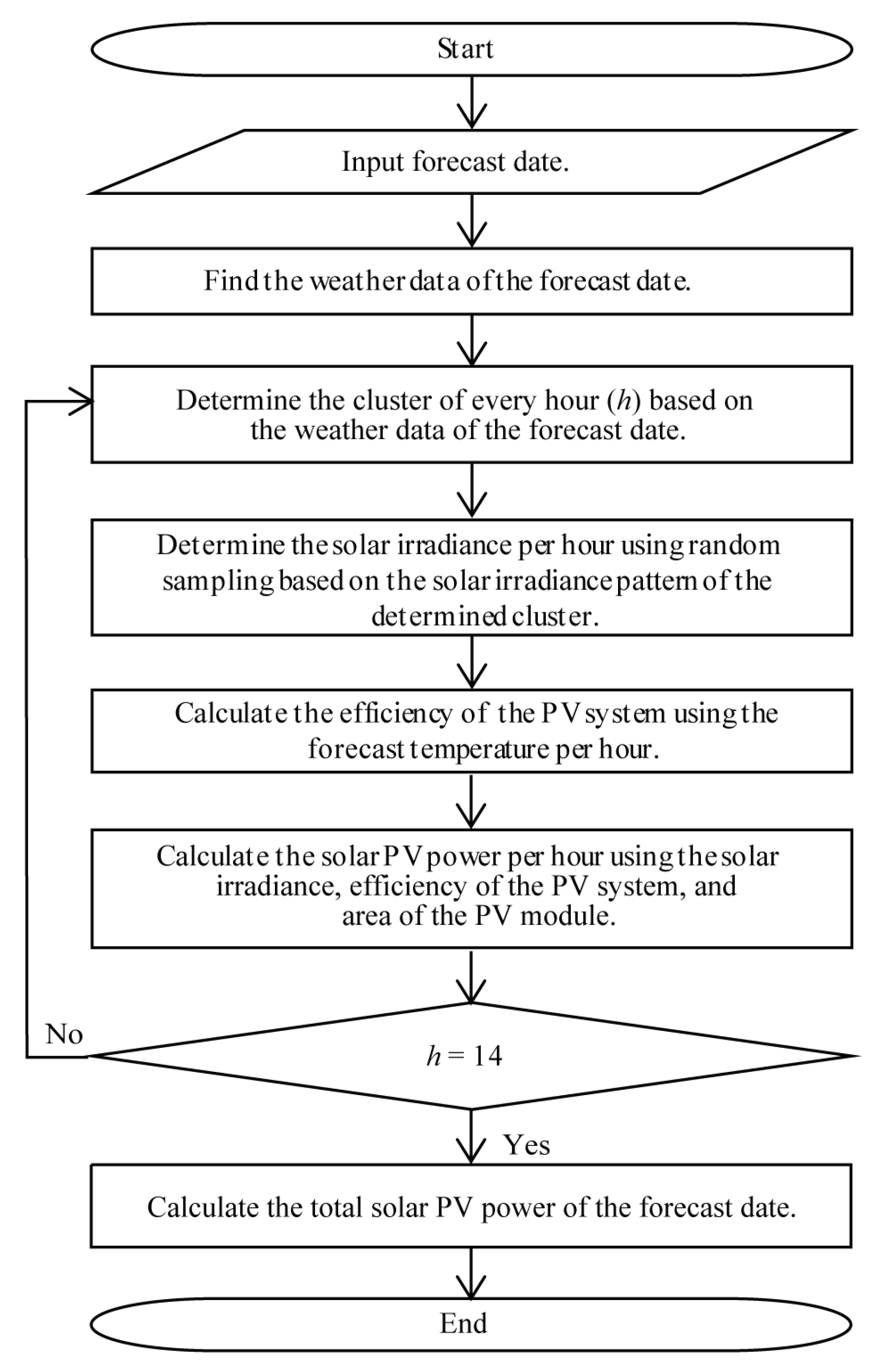
2.3.5. Flowchart of the Solar PV Power Prediction Model

The flowchart of the solar PV power prediction model in this paper is shown in Figure 4. The program starts after the forecast date, which includes the month and the day, is entered. The computer program finds the weather data of the forecast date from the stored historical data from the local disk. From the forecast weather data, the computer program determines the cluster of every hour from 5:00 to 18:00 of the forecast date. The solar irradiance per hour is determined using random sampling based on the pdfs in (13)–(16) of the solar irradiance pattern of the determined cluster per hour. The efficiency of the PV system is calculated using the forecast temperature per hour using (17). The solar PV power is calculated using the determined solar irradiance per hour using random sampling, the calculated efficiency of the PV system, and the area of the PV module of the PV system using (18). The solar PV power is calculated until the number of hours (h) is equal to 14, which is the number of hours from 5:00 to 18:00. The output is the solar PV power profile from 5:00 to 18:00 of the forecast date.

3. Results

This section provides numerical examples to illustrate the proposed solar PV power prediction model presented in Section 2. In this paper, the historical data, which include the solar PV power, solar irradiance, and weather data, are used to formulate the solar PV power prediction model and are from the month of January, which is a summer season in Australia. Only one season is considered for the limitation of this paper because presenting all the seasons would make the paper redundant in terms of processing the data. The summer season is chosen to determine the impact of other weather data on solar irradiance when solar irradiance is highest. Nevertheless, the proposed solar PV power prediction may be used to predict any day in all the seasons given that the historical data used to formulate the prediction model is from the month to be forecasted. To show the effectiveness of the prediction model, the solar PV power of the whole month of January 2017 are forecasted and compared to the actual solar PV power.

From the different techniques and methods in forecasting solar PV power presented in previous studies [4,5,6,7,8,9,10,11,12,13,14,15,16,17,18,19,20,21,22,23], big data tools have not been applied. This paper formulates a solar PV power prediction model using big data tools. Compared with previous studies [8,9,11], this paper also considers humidity, wind speed, precipitation, cloudiness, and weather condition, together with the temperature as the weather data used in formulating the solar PV power prediction model. In addition, this paper calculates the solar PV power using the following assumptions:

• The solar irradiance per hour is assumed to be a random variable that follows a Normal, Exponential, Rayleigh, or Kernel distribution, of which each parameter is calculated using the historical solar irradiance per hour of the month of January from 2012 to 2016.
• The efficiency of the PV system is based on the temperature of the forecast day.

In addition, the root mean square error (RMSE) and the mean relative error (MRE) were used to verify the effectiveness of the proposed solar PV power prediction model in this paper. The RMSE, which is the total error in the entire duration of the prediction period, was chosen because it is one of the common evaluation indices used to determine the accuracy of the solar PV power prediction model [3]. In this paper, the accuracy error of the solar PV power prediction model is expressed in solar PV power in terms of kW. Moreover, the MRE was also used to verify the performance of the proposed solar PV power prediction model to compare the obtained result to previous studies. The MRE was also chosen as the evaluation index in this paper because it is reasonable to divide the difference of the actual and forecast solar PV power by the total power capacity of the PV system that shows a practical impact. In this paper, the actual and forecast average solar PV power values for every hour from 5:00 to 18:00 were considered in computing the RMSE and the MRE given in (19) and (20), respectively:

$$RMSE=\sqrt{\frac{1}{N}\sum _{i=1}^N{\left(P_A-P_F\right)}^2},$$

(19)

$$MRE=\frac{1}{N}\sum _{i=1}^N\left|\frac{P_A-P_F}{P_T}\right|\times 100,$$

(20)

where P_A is the actual average solar PV power, P_F is the forecast average solar PV power, P_T is the total power capacity of the PV system (i.e., 433.44 kW), and N is the number of forecast hours from 5:00 to 18:00 (i.e., 14).

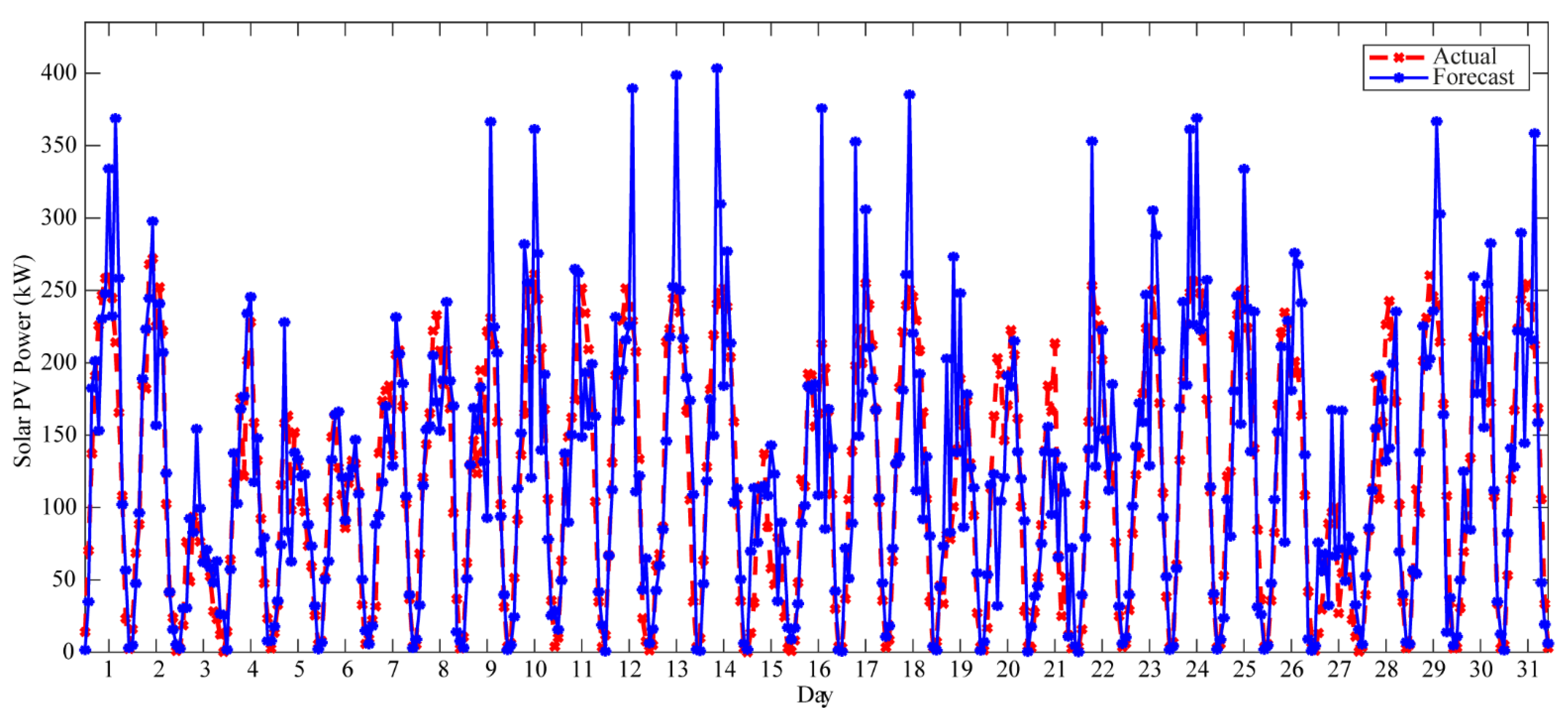
Figure 5 shows the solar PV power profiles of each day of January 2017 obtained using the proposed solar PV power prediction model. The whole month of a summer season was chosen to show the variability of the solar PV power profile in each day. To show the accuracy of the forecast values, the actual and the forecast solar PV power profiles from 5:00 to 18:00 for each day of January 2017 were compared as depicted in Figure 5.

In addition, the parameters which describe the forecast solar PV power in Figure 5 are listed in

Table 2. The average and maximum forecast solar PV power and the time with maximum solar PV power for each day of January 2017.

Day	Average Solar PV Power (kW)	Maximum Solar PV Power (kW)	Time with Maximum Solar PV Power	Day	Average Solar PV Power (kW)	Maximum Solar PV Power (kW)	Time with Maximum Solar PV Power
1	171.97	368.84	14:00	17	138.00	352.73	9:00
2	135.37	297.72	11:00	18	144.23	385.21	11:00
3	60.54	154.29	10:00	19	116.25	273.21	10:00
4	110.99	245.57	12:00	20	106.91	215.10	14:00
5	86.67	228.03	8:00	21	78.289	155.83	10:00
6	97.54	166.28	10:00	22	123.826	353.00	9:00
7	110.31	231.56	13:00	23	139.320	305.24	13:00
8	129.16	242.02	14:00	24	177.553	369.04	12:00
9	131.95	366.48	13:00	25	129.147	333.83	12:00
10	146.64	361.36	12:00	26	138.573	276.00	13:00
11	135.12	264.90	10:00	27	68.370	167.50	10:00
12	138.91	389.49	13:00	28	114.358	235.40	15:00
13	154.32	398.67	12:00	29	143.351	366.73	13:00
14	153.78	403.36	10:00	30	132.994	282.56	15:00
15	77.46	143.07	12:00	31	145.51	358.47	14:00
16	122.44	375.71	13:00

to provide information on the forecast solar PV power. As shown in Figure 5 and as listed in Table 2, the maximum solar PV power with 403.36 kW is observed on 14 January 2017, which also has the highest average temperature of 31.5 °C. This indicates that temperature has a significant impact on the generated solar PV power. In contrast, the lowest average solar PV power per day of 60.54 kW was observed on 3 January 2017. This is because the lowest average temperature of 24.79 °C, the highest average humidity of 86.93%, and the highest percentage of being cloudy of 99.29% were also forecast on this day (i.e., 3 January 2017). This shows that having the highest humidity and the highest percentage of being cloudy results in a reduced amount of solar radiation received by the PV module. Moreover, the maximum solar PV power for each day was observed at different times, which is caused by different factors. As observed in Table 1, different factors significantly affect the solar irradiance per hour which also affects the solar PV power. The variation in the time of having the maximum solar PV power for each day shows that the solar PV power varies with weather data (i.e., temperature, humidity, wind speed, precipitation, cloudiness, and weather condition) per hour and not with the day of the week.

As observed in Figure 5, the actual solar PV power and the forecast solar PV power show some discrepancies. These discrepancies are from the stochastic nature of the solar irradiance determined using the pdfs in (13)–(16), which were used as a parameter in the calculation of the solar PV power. To show the accuracy of the solar PV power prediction model,

Table 3. Root mean square error (RMSE) and mean relative error (MRE) of each day of January 2017.

Day	RMSE (kW)	MRE (%)	Day	RMSE (kW)	MRE (%)
1	58.87	9.50	17	53.96	8.55
2	25.52	4.34	18	57.08	9.39
3	29.51	5.26	19	63.11	8.78
4	25.71	5.03	20	58.20	9.01
5	33.71	5.51	21	47.01	7.49
6	17.57	2.80	22	49.83	8.31
7	27.71	4.48	23	37.89	6.78
8	33.73	5.81	24	53.63	8.68
9	52.97	7.14	25	49.83	8.98
10	53.31	9.18	26	57.08	8.75
11	48.29	8.63	27	47.82	8.78
12	56.40	8.80	28	48.89	7.79
13	52.13	7.56	29	55.52	9.07
14	56.76	8.83	30	48.32	8.43
15	46.01	8.52	31	55.49	8.83
16	57.01	8.12

shows the RMSE and MRE results that are determined by comparing the actual and forecast average solar PV power per hour for each forecast day of January 2017. As listed in Table 3, the best RMSE and MRE of 17.57 kW and 2.80% was obtained on 6 January 2017, which shows relatively accurate results obtained from the proposed solar PV power prediction model. This result also shows an improved MRE result obtained in evaluating the performance of the solar PV power prediction model compared to MRE results obtained in the solar PV power prediction model in previous studies [12,22]. Therefore, the result of this proposed solar PV power prediction model may provide information on the shortage and excess of solar PV power generation. Furthermore, the proposed solar PV power prediction model may help in generation planning for reliable integration into the grid and a stand-alone PV system.

4. Discussion

A solar PV power prediction model using big data tools was presented in this paper. The historical solar PV power, historical solar irradiance, and historical weather data (i.e., temperature, humidity, wind speed, precipitation, cloudiness, and weather condition) were used in the formulation of the solar PV power prediction model. These historical data were stored, managed, and processed using big data tools. The solar irradiance, efficiency of the PV system, and the area of the PV module in the PV system were considered in the calculation of the solar PV power in this paper.

The solar PV power profile of each day of January 2017 was presented in numerical examples to show the variability of the solar PV power profiles in a summer season. The solar PV power of the whole month of January 2017 can only be forecast since the historical data used in formulating the solar PV power prediction model are from the month of January from 2012 to 2016. Although solar PV power prediction was formulated using the historical data of January from 2012 to 2016, it can still be used in predicting the solar PV power of the future. Nevertheless, the proposed solar PV power prediction method may be used to predict any day in all the seasons given that the historical data used to formulate the prediction model is from the month to be forecasted.

The results of the presented solar PV power prediction model show that the maximum solar PV power value varies with time based on the factors (i.e., weather data) that affect the solar irradiance. This shows that it is important to determine the factors that significantly affect the solar irradiance per hour to accurately illustrate the solar PV power profile for each day. In addition, the day with the highest average temperature per day appeared to have the highest average solar PV power per day. Meanwhile, the day that shows the lowest average solar PV power per day was observed to have the lowest average temperature, highest average humidity, and the highest percentage of being cloudy per day. This is because the humidity and cloudiness reduced the solar radiation reception of the PV module in the PV system.

Moreover, the performance of the presented solar PV power prediction model was also verified using RMSE and MRE results obtained by comparing the actual and forecast average solar PV power per hour. The best RMSE and MRE results of 17.57 kW and 2.80%, respectively, were obtained using the presented solar PV power prediction model that has a lower MRE result compared to the MRE results obtained by the solar PV power prediction model of previous studies. The results of the presented solar PV power prediction model provide relatively accurate forecasting of solar PV power.

Therefore, the solar PV power profiles obtained using the presented solar PV power prediction model may provide information on the availability of solar PV power generation. Furthermore, the presented solar PV power prediction model may help in generation planning for reliable integration of solar PV systems to the grid and provide reliable power to a stand-alone network.