
Risk Assessment Models to Improve Environmental Safety in the Field of the Economy and Organization of Construction: A Case Study of Russia


Abstract
1. Introduction
1.1. Objectives
- To develop scenarios for the development of risky situations, identify their parameters, evaluate each scenario and compare them;
- To analyze the characteristics of each risk scenario;
- To identify the most significant risks affecting the development of the scenarios under consideration;
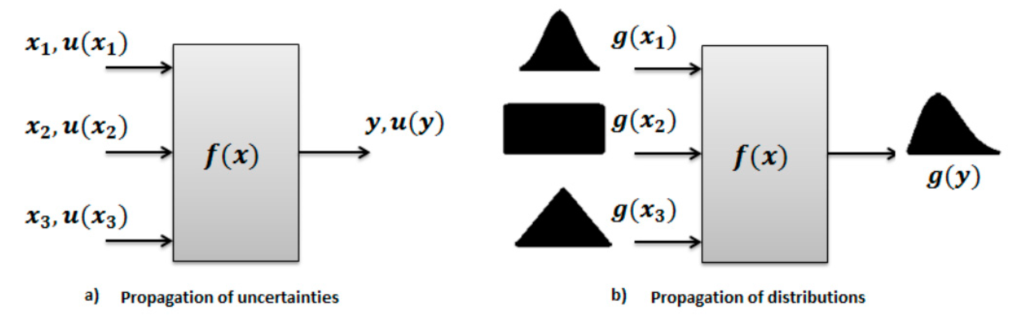
- To apply the objective methods of Monte Carlo assessment (logistics and lognormal distributions as risk analysis tools);
- To conduct studies to form a complete algorithm and methods for use in environmental safety and construction.
1.2. The Use of the Monte Carlo Method
- A uniform distribution if only the upper and lower bounds of the values are known;
- An exponential distribution if only the lower bound and the mean are known;
- A normal distribution if only the mean and standard deviation are known.
1.3. EIA as an Assessment of the Technogenic Impact on the Environment
- Federal Law of Russia FZ-7. On Environmental Protection, 2002, https://docs.cntd.ru/document/901808297 (accessed on 24 November 2021);
- Federal Law of Russia FZ-174. On Environmental Expertise, 1995, https://docs.cntd.ru/document/9014668?section=text (accessed on 24 November 2021);
- Order of the State Committee for Ecology of Russia dated May 16, 2000 FZ-372 On approval of the Regulation on assessing the impact of planned economic and other activities on the environment in the Russian Federation, https://base.garant.ru/12120191/ (accessed on 24 November 2021);
- GOST R 54135-2010 Environmental management. Guidance for organizational safeguards application and risk assessment. Native zone protection. General aspects and monitoring, https://docs.cntd.ru/document/1200086159?section=status (accessed on 24 November 2021);
- Methodology of the Ministry of Energy of Russia. Methodology for determining damage to the environment in case of accidents on oil trunk pipelines, 1995, https://docs.cntd.ru/document/1200031822?section=status (accessed on 24 November 2021);
- Safety Guidelines. Methodological recommendations for conducting a quantitative analysis of the risk of accidents at hazardous production facilities of main oil pipelines and main oil product pipelines, 2016, https://docs.cntd.ru/document/456007201?section=status- (accessed on 24 November 2021).
- The United States Environmental Protection Agency (EPA/2021): Use of Monte Carlo Simulation in Risk Assessments, https://www.epa.gov/risk/use-monte-carlo-simulation-risk-assessments (accessed on 24 November 2021);
- The United States Environmental Protection Agency (EPA/100/B-04/001 March 2004): An Examination of EPA Risk Assessment Principles and Practices, https://semspub.epa.gov/work/10/500006305.pdf (accessed on 24 November 2021);
- The Society for Risk Analysis (SRA/2018): Risk Analysis Fundamental Principles, https://www.sra.org/wp-content/uploads/2020/04/SRA-Fundamental-Principles-R2.pdf (accessed on 24 November 2021).
1.4. Study Objectives in the Context of Risk Assessment
- IEC/FDIS 31010 Risk Management—Risk Assessment Techniques, https://bambangkesit.files.wordpress.com/2015/12/iso-31010_risk-management-risk-assessment-techniques.pdf (accessed on 24 November 2021).
- ISO/IEC 31010: 2009 Risk Management—Risk Assessment Techniques, https://www.iso.org/standard/51073.html (accessed on 24 November 2021).
- ERM/COSO Enterprise Risk Management—Integrated Framework, https://www.coso.org/Pages/erm-integratedframework.aspx (accessed on 24 November 2021).
- EOSCA Chemical Hazard Assessment and Risk Management, https://eosca.eu/wp-content/uploads/2018/08/CHARM-User-Guide-Version-1-5.pdf (accessed on 24 November 2021).
- GOST R 51897-2011 Risk Management. Terms and Definitions, https://docs.cntd.ru/document/1200088035 (accessed on 24 November 2021).
- GOST R 58771-2019 Russian State Standard: Risk Management. Risk Assessment Technologies, https://docs.cntd.ru/document/1200170253 (accessed on 24 November 2021).
1.5. Research Novelty
2. Literature Review
3. Materials and Methods
4. Results
- P is the probability of emergencies occurrence;
- C is the expected damage and consequences in the event of an accident.
- Monitoring the assessment of the technical condition of system elements;
- Carrying out and providing organizational and technical solutions aimed at improving the quality and reliability of the system, and ultimately, at a significant improvement in the state of the environment at the construction site;
- Developing methods for operational control of the system’s operating modes;
- Providing the system with qualified personnel;
- Attracting investments to improve the safety of the system’s operation.
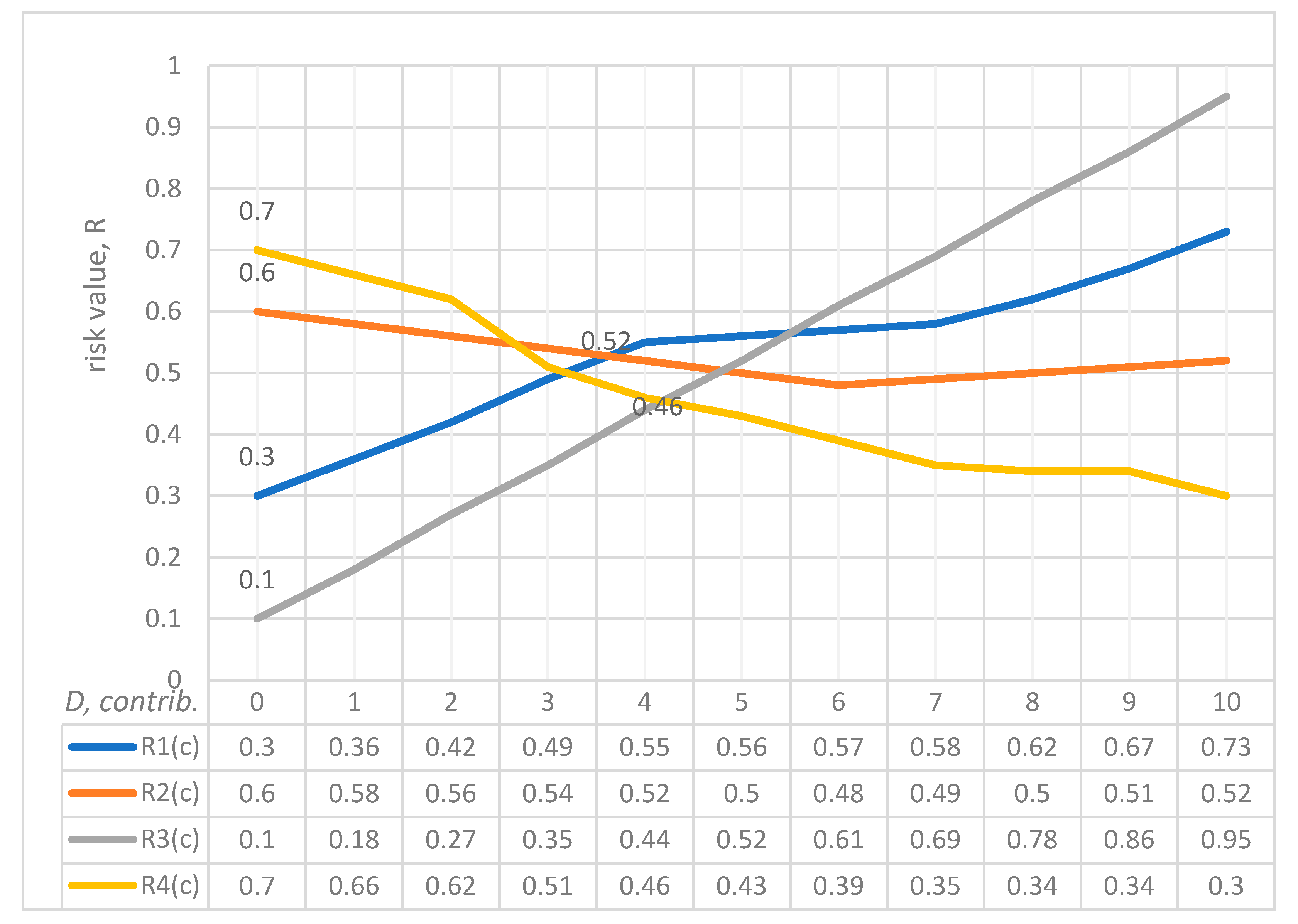
- Scenario 1. The facility’s placement caused a change in the landscape, meaning there is a risk of destruction by flooding; the probability P1 = 0.3. According to Formula (9), despite an object’s low risk, its location must be considered (Scenario 1 states that the placement of the object caused the terrain to change. The object itself is not dangerous as such (the anthropogenic factor, in this case, is excluded). However, the object can still be destroyed (the natural factor is considered) due to changes in the landscape. Therefore, the destruction of an object depends directly on its location, which must be considered). The amount of funds (s1) aimed at preventing emergencies and environmental safety measures does not provide a low-risk value a priori due to the possibility of a landscape disturbance (for example, flooding). The investment of s2 funds in maintaining the reliability of the technical system may be unjustified due to the negative effects of external factors, which leads to a pessimistic, unfavorable scenario rather than one that has a relatively low-risk value.
- Scenario 2. The construction did not meet the parameters of design documentation due to a building violation—namely, failure to install fire extinguishing equipment, and the risk of fire is a likelihood; the probability P2 = 0.6. According to Formula (9), a high risk of emergencies always arises when project parameters are violated, despite the high investment s2 in the safety of the technical system.
- Scenario 3. The design costs of construction for this area did not consider the parameter of seismic safety; therefore, there is a risk of damage or destruction of the facility during an earthquake; the probability P3 = 0.1. According to Formula (9), given the values of s1 and s2 and a low value of risk, it is important to understand what is relevant in a scenario associated with a place that has a potential seismic hazard. For example, in St. Petersburg (Russia), the possibility that events in a seismic safety scenario could develop is non-existent. However, in Tbilisi (Georgia), the damaging factors of an earthquake can reach the scale of a natural disaster.
- Scenario 4. The facility is associated with an environmentally hazardous technological process and can cause an emergency at any time; the probability P4 = 0.7. According to Formula (9), it should be noted that when in full compliance with the requirements for the technological process and corresponding investments (s2) in the safety of the technical system, emergencies with a high value of risk are impossible, and the development of this scenario is likely to be optimistic. In choosing between s1 (funds allocated for the prevention of emergencies and environmental safety measures), and s2 (funds allocated for the failure-free operation of the technical system), the optimal scenario will be the one that ensures the technical safety of production.
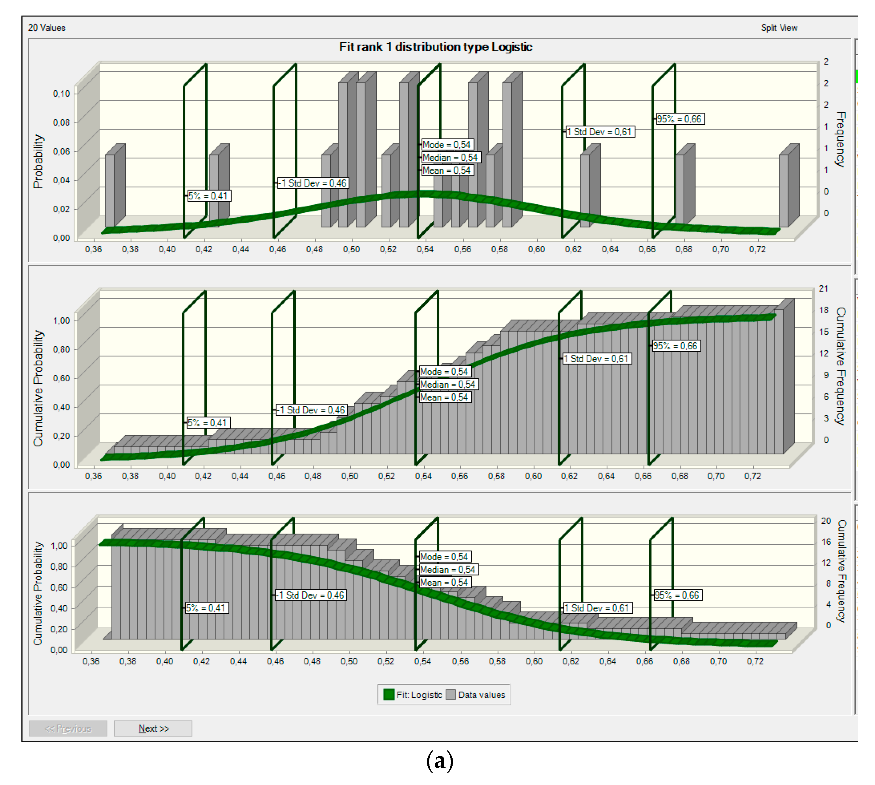
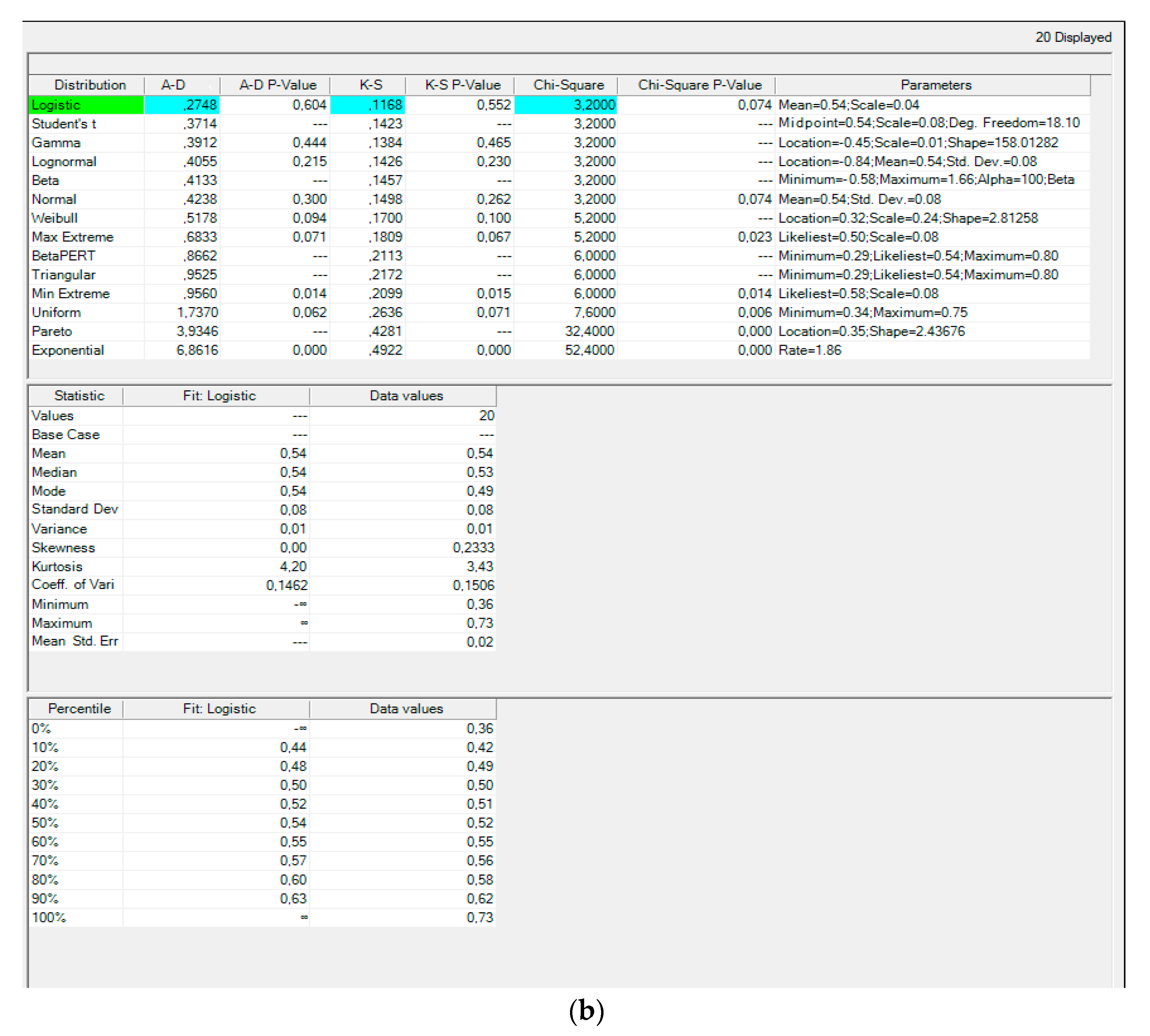
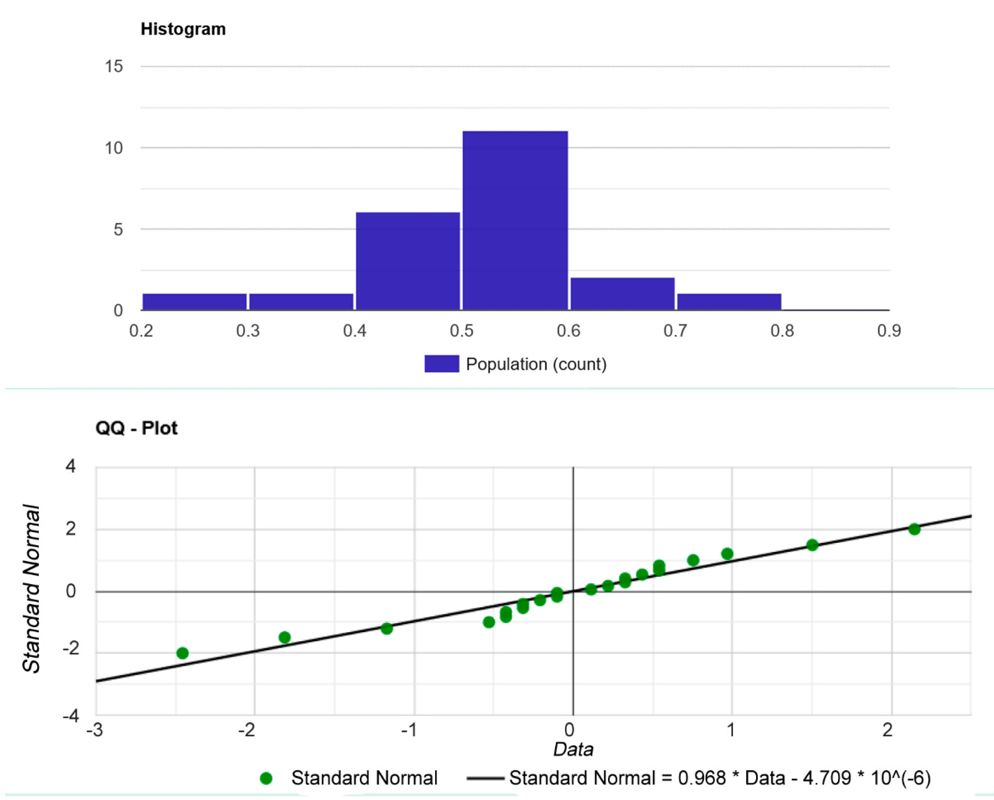
- Hypothesis H0: since the p-value > α, it needs to take H0. The data are assumed to be normally distributed. In other words, the difference between a sample of data and a normal distribution is not large enough to be statistically significant;
- p-value. The p-value is 0.411559. Therefore, if H0 is rejected, the probability of type 1 error (deviation of the correct H0) would be too high: 0.4116 (41.16%);
- W Statistic: 0.955926. It is within the acceptable range of 95% of the critical value: [0.9112: 1.0000];
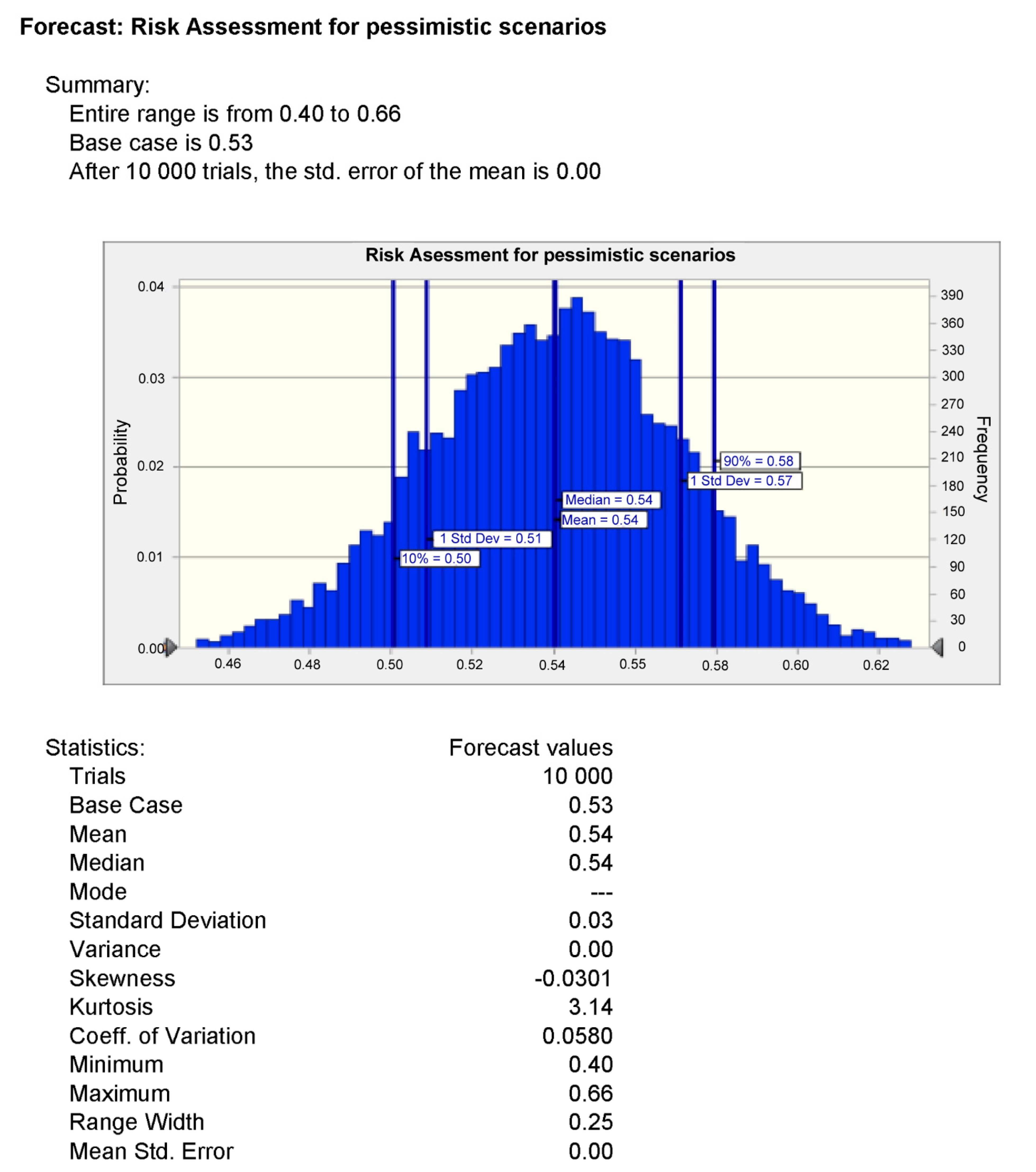
- Median: 0,53. Average (x): 0.529545. Sample standard deviation (S): 0.0934766. Sample size (n): 22. Skewness: −0.403046. Excess kurtosis: 1.395218.
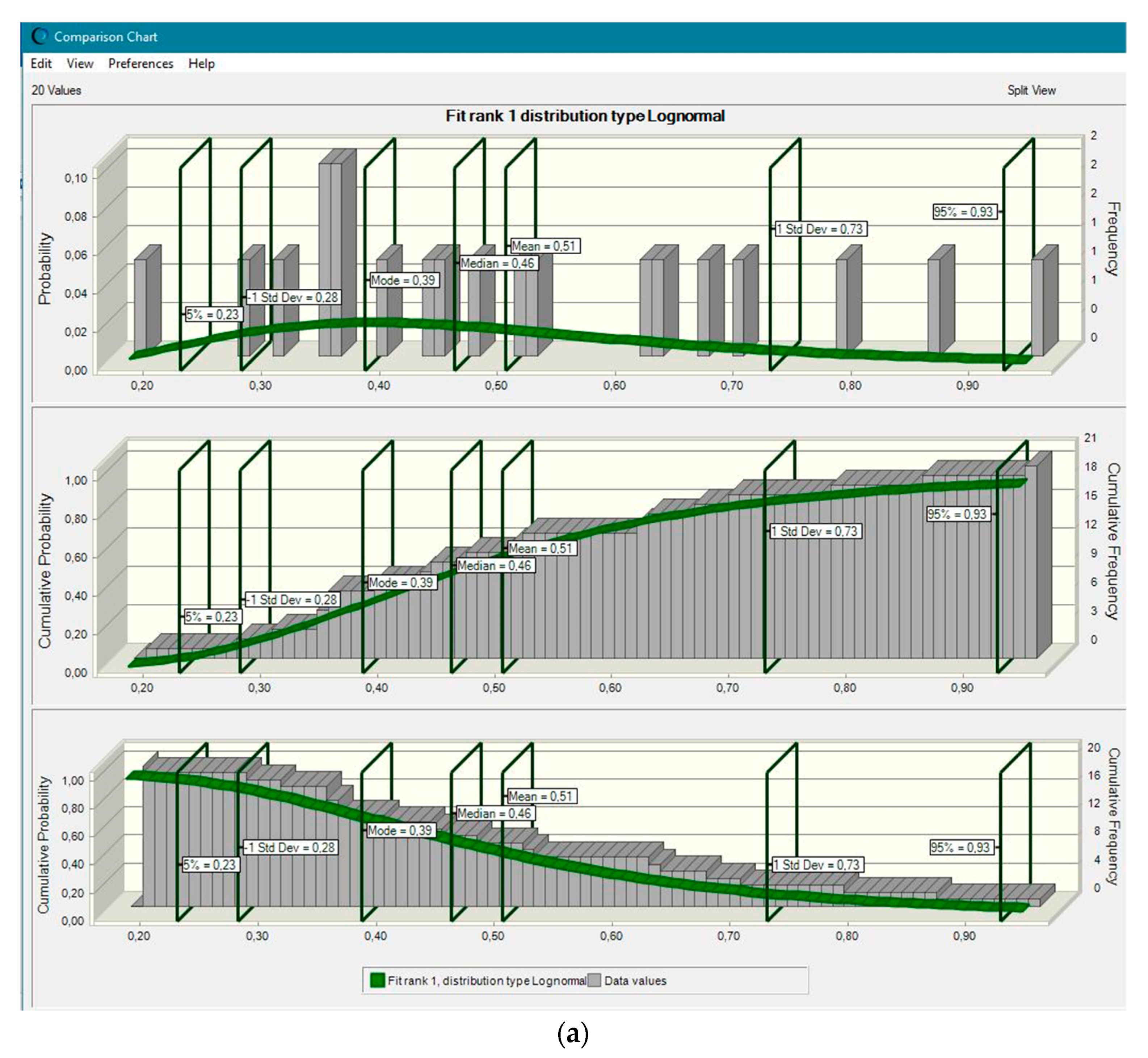
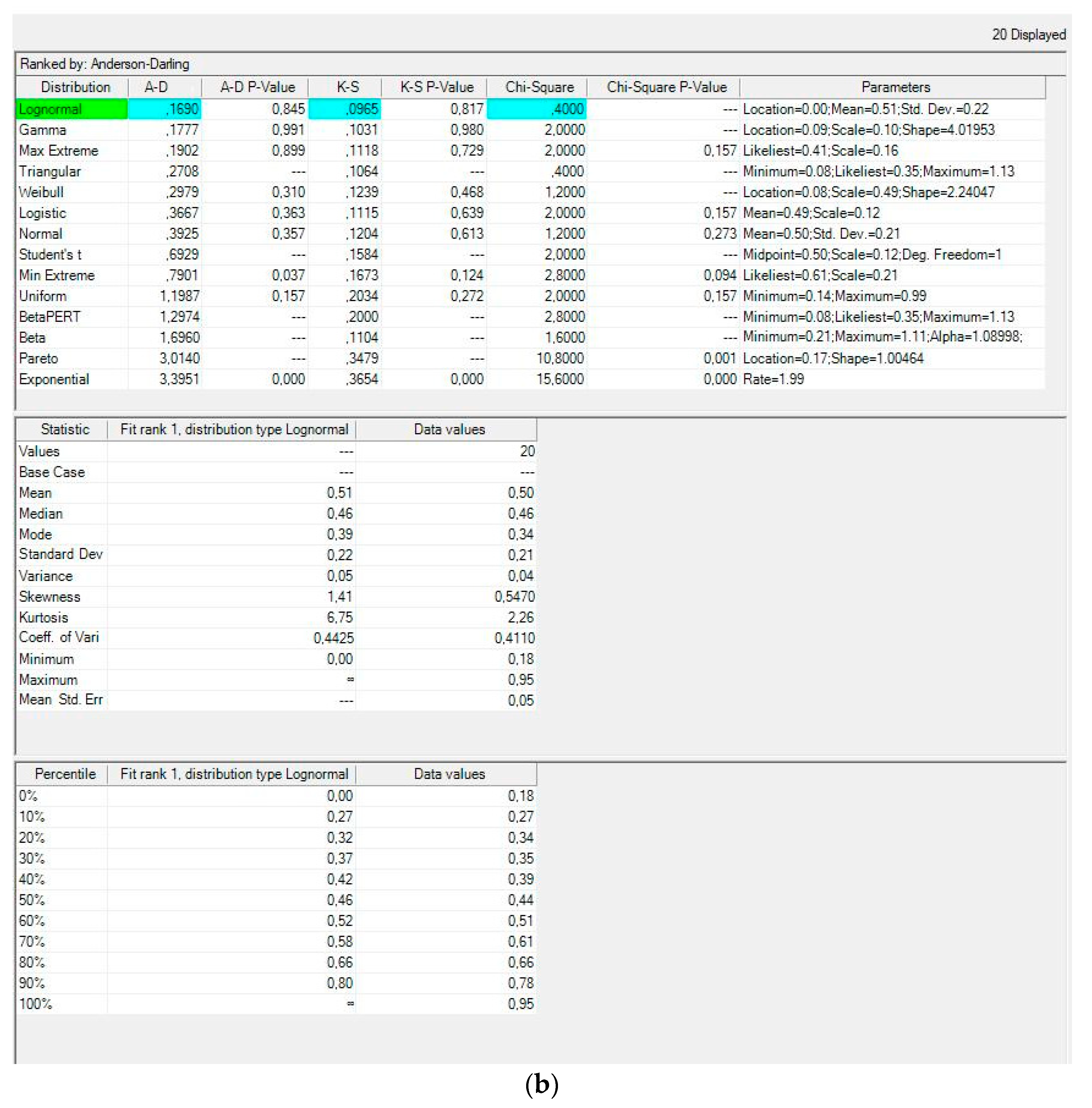
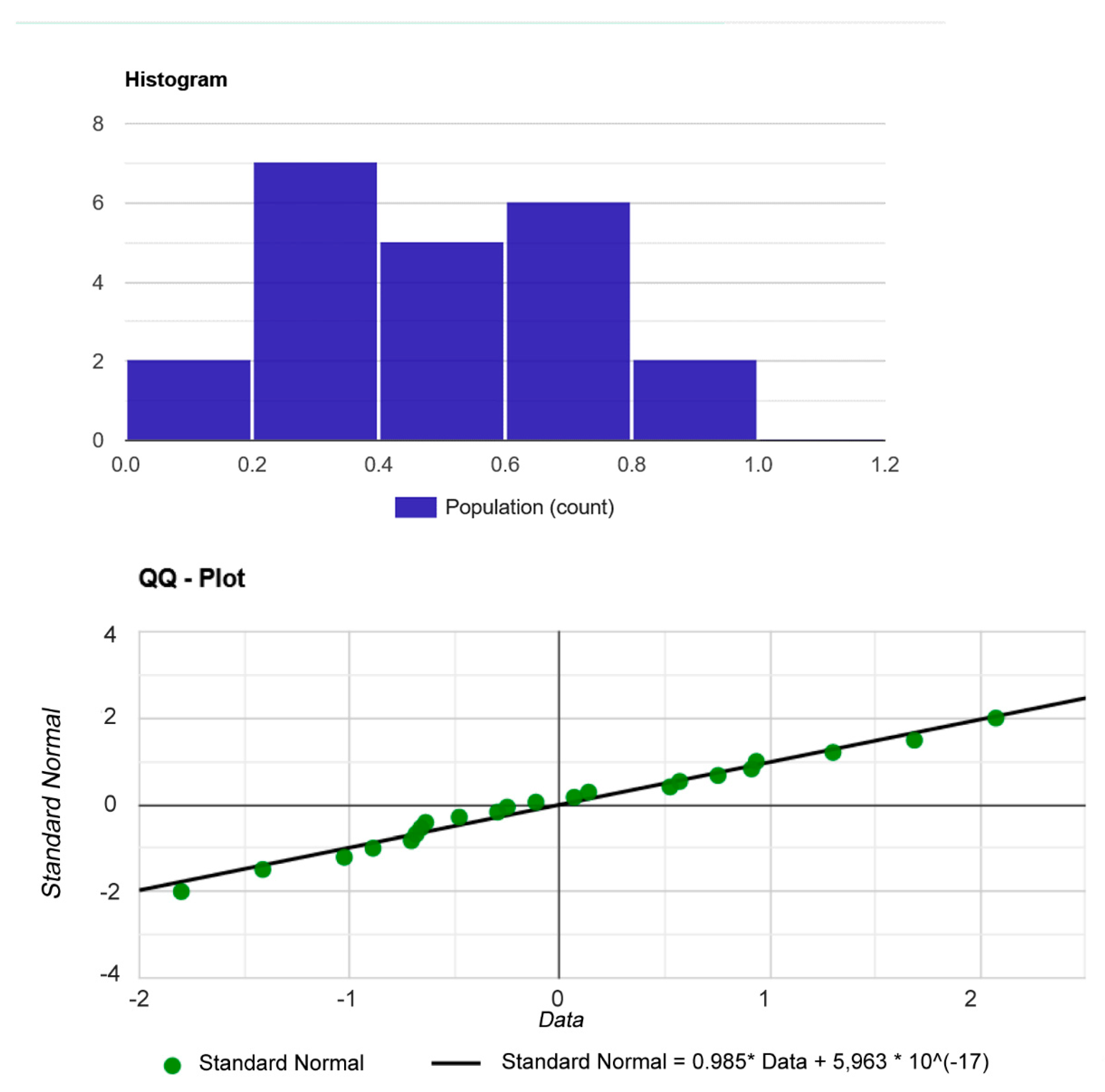
- Hypothesis H0: since the p-value > α, it needs to take H0. The data are assumed to be normally distributed. In other words, the difference between a sample of data and a normal distribution is not large enough to be statistically significant;
- p-value. The p-value is 0.875764. Therefore, if H0 is rejected, the probability of type 1 error (deviation of the correct H0) would be too high: 0.8758 (87.58%);
- W Statistic: 0.977658. It is within the acceptable range of 95% of the critical value: [0.9112: 1.0000];
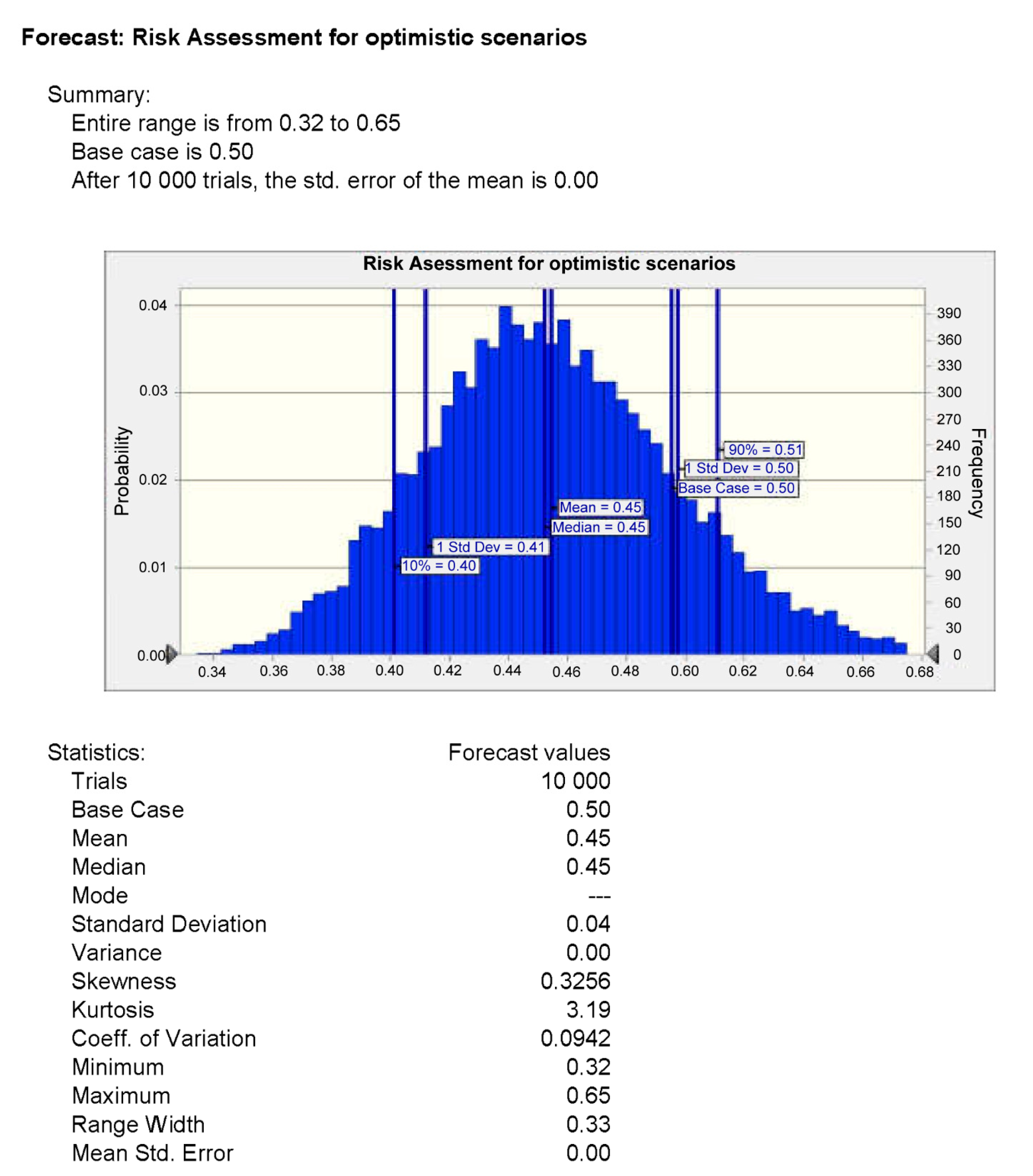
- Median: 0.45499999999999996. Average (x): 0.495000. Sample standard deviation (S): 0.219437. Sample size (n): 22. Skewness: 0.336493. Excess kurtosis: −0.408523.
5. Discussion
6. Conclusions
Author Contributions
Funding
Institutional Review Board Statement
Informed Consent Statement
Data Availability Statement
Acknowledgments
Conflicts of Interest
Appendix A. Notes
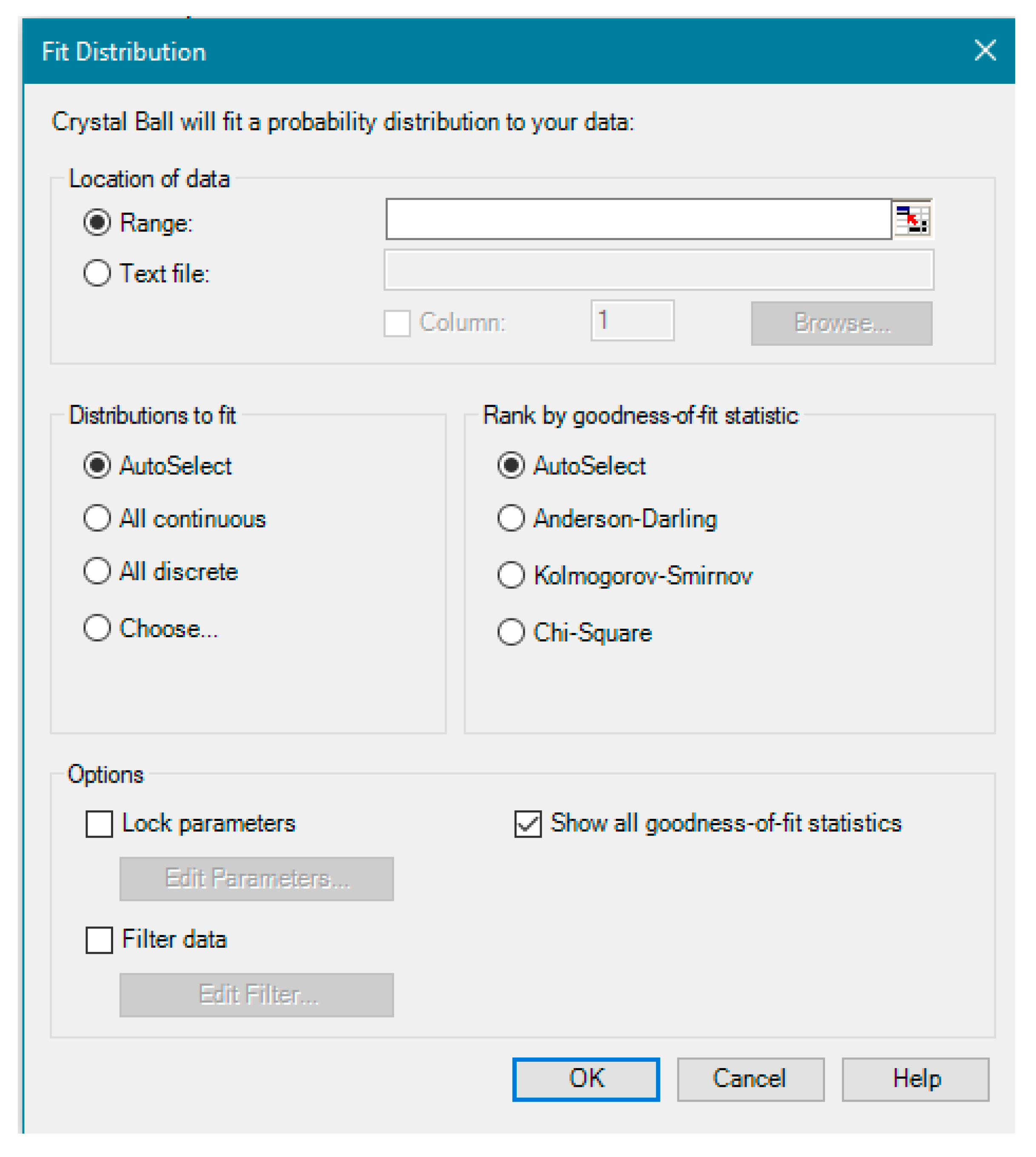
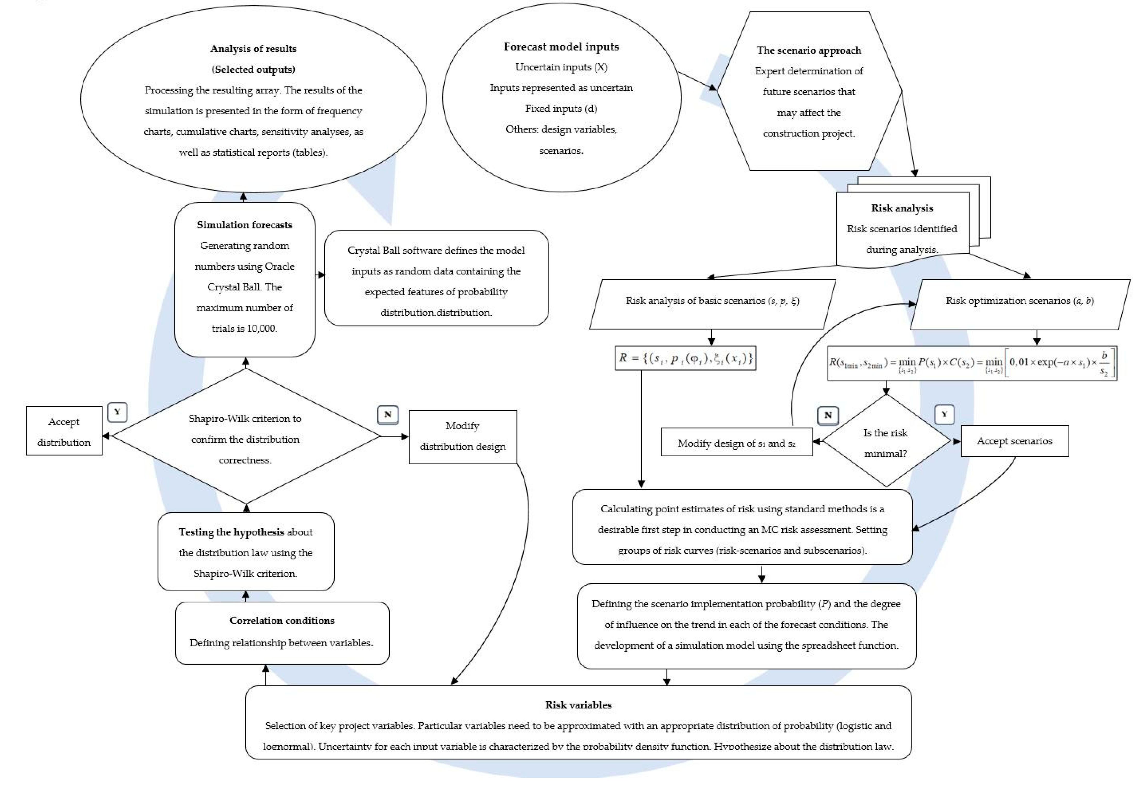
- In practice, carrying out a quantitative assessment of risks, the following basic classification of methods is repeatedly used: statistical (to assess the probability of a random event occurring based on the relative frequency of occurrence of this event in a series of observations); analytical (to study functional dependence, modeling with probabilistic indicators); expert assessments (to analyze quantitative and qualitative groups of factors). The above qualitative and quantitative methods are used in the instruments of this classification. For example, the Monte Carlo method can be defined as an analytical method for modeling random variables to calculate the characteristics of their distribution; it is the construction of an artificial random process using conventional computing means. However, the main problem with using a classical scenario analysis for risk assessment is that the large number of possible combinations that can affect the resulting project performance indicator tends to infinity. Solving this problem is one of the main advantages of Monte Carlo simulation. However, such modeling refers to statistical methods, because knowing the distribution laws of variables, it is possible to obtain not a single value but the distribution of the resulting indicator for an unlimited number of different scenarios.
- What is an environmentally friendly construction option? Any construction is unsafe and poses a threat to the environment. This is about minimizing the risk of negative impact by the natural and anthropogenic factors of an environmental hazard. The method of work represents several measures that provide, with a given probability, an admissible negative impact by these factors. Risk should always be viewed in the context of a decision scenario. Then, a risk accompanied by the best solution is acceptable. In our opinion, all other risks are unacceptable, even if they are less risky. This is an environmentally friendly construction option.
- This definition is formulated in the current document adopted by the Federal Agency for Technical Regulation and Metrology. The state standard itself (i.e., GOST) was prepared by the Scientific Research Center for Control and Diagnostics of Technical Systems, submitted for consideration by the Technical Committee for Standardization TC 10 “Risk Management”. The standard is identical to ISO Guide 73: 2009 “Risk management—Vocabulary—Guidelines for use in standards”, IDT).
- The statement “Ordinarily, construction must consider the multidimensional nature of the impact on environmental components” indicates the multidimensional nature of the environmental hazard. According to this article, several scenarios are considered that deal with natural and anthropogenic impacts on the environment. The multidimensional nature of an environmental hazard is attributed to several factors and has many properties because both the natural environment and the technogenesis itself are multidimensional, and together, they form some natural and technical system on a certain territory. In turn, the multidimensionality of a natural–technical system is determined by the number and difference of types of natural and artificial objects that give the entire system the specific properties of a multidimensional whole. As for the components of the natural environment, these are earth, subsoil, soils, surface and underground waters, atmospheric air, flora, fauna, and other organisms, as well as artificial objects that together provide favorable conditions for the existence of life. Any change in the parameters of the state of an environmental component at one of its levels of organization causes changes in all of its hierarchical levels. The lists of environmental components, whose descriptions are necessary for decision making, generally depend on the type of planned activity and the expected impacts. Indicative lists of this kind may be found in departmental instructions or corporate guidelines. An important role in clarifying which natural conditions and environmental components need to be described for a given type of project can be played by a scenario approach for assessing their environmental safety.
- According to the “Methodological fundamentals for the analysis of hazards and risk assessment of accidents at hazardous production facilities” (Russia, 2016, https://docs.cntd.ru/document/1200133801 (accessed on 24 November 2021)), environmental damage for various potentially hazardous industrial and construction sites or projects is estimated as the sum of losses inflicted by each type of environmental pollution according to the following formula:where ECA is compensation for damage from air pollution; ECG is compensation for damage from the pollution of water bodies (hydrosphere); ECL is for damage from soil pollution (lithosphere); ECB is for damage from biosphere pollution; ECW is for damage caused to the territory by construction waste. The answers to the question (1) who is compensated and (2) from whom are as follows: (1) representatives of the state technical supervision of Russia who monitor the operation of hazardous facilities and assess the damage caused to the environment due to accidents at hazardous production facilities; (2) law offenders, employees of organizations, operating hazardous production facilities
- It can be stated that the probability is not determined statistically or mathematically but based on how the conditions are analyzed for the design, construction, and operation of the facility. This is partly true since each method of analysis has some limitations in terms of the results obtained; however, the likelihood certainly does not depend solely on the method of analysis used. The probability assessment is a purely systemic issue. The scenario approach was introduced so that a deterministic description of the probability of risk would be neither practically possible nor expedient. Risk assessment includes the entire range of methodological tools and the entire context in which it is structured and implemented. The mathematical and statistical probability is only a part of the specified context of estimation. Does risk analysis involve establishing causal relationships between a hazardous event and its sources and consequences? Of course. Yes. Is probability related to the frequency of the occurrence of events? Of course, yes. This is its “empirical” definition. Thus, it is often said that we cannot use probability because we do not have enough data. Considering the current definitions, we can see that this is misleading. When there are not enough data, there is no choice but to use probability. Therefore, it could be said that probability, as a science that works with a lack of data, fits methodologically into our research well. Risk should not be thought of as acceptable or in isolation but only in conjunction with the costs and benefits that come with this risk. Viewed in isolation, no risk is tolerable. The rational person will not take any risk at all, except, perhaps, in return for the benefits that come with it.
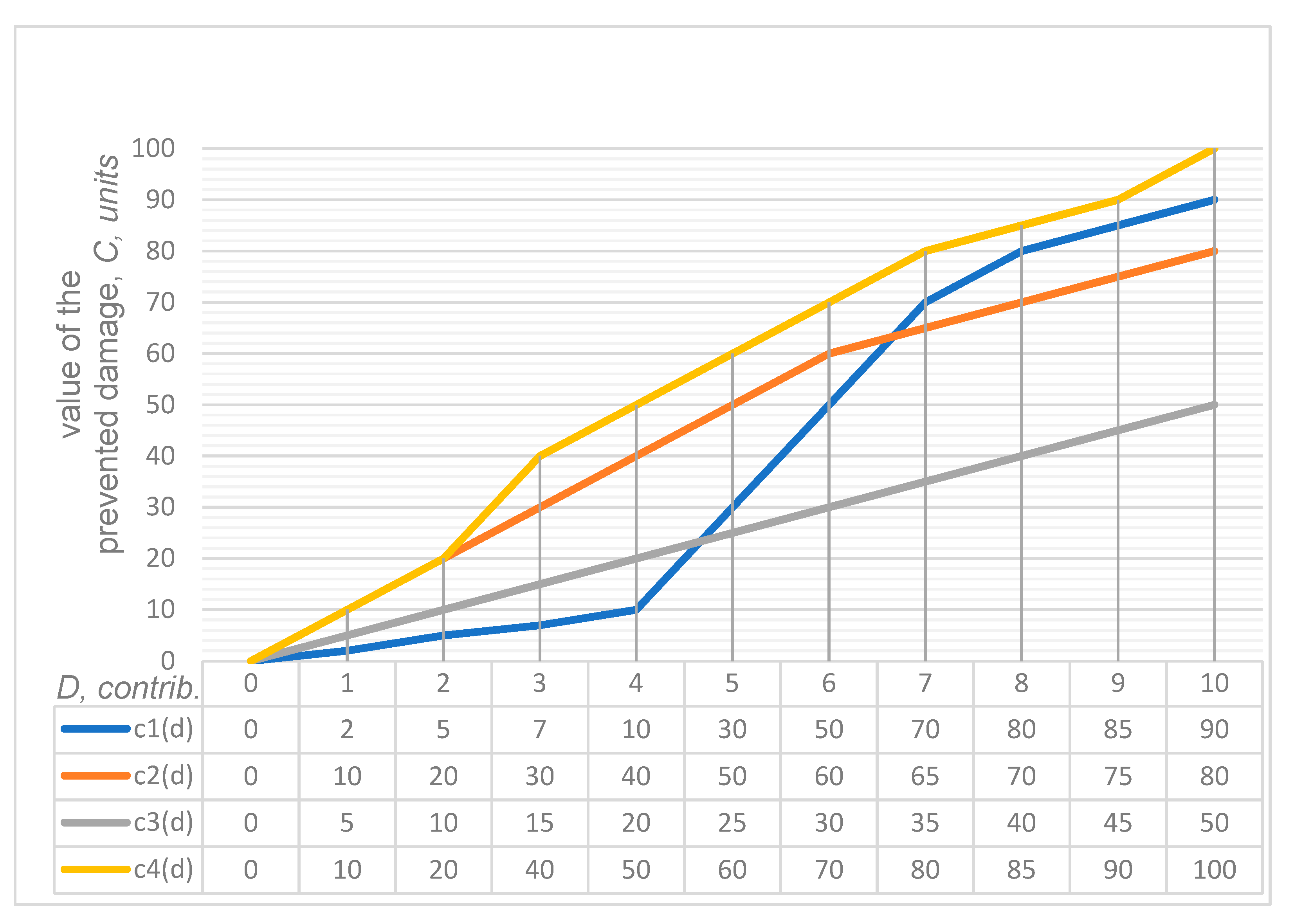
- Initial data are based on the following Russian guidelines:“Methodological recommendations for risk assessment accidents of hydraulic structures reservoirs and storages of industrial waste”, N 9-4/02-644 of 14.08.2001, developed by the Research Institute “VODGEO” (Moscow), https://70.mchs.gov.ru/uploads/resource/2021-07-16/metodicheskie-rekomendacii-mchs-rossii_16264287321541523919.pdf (accessed on 24 November 2021).“Methodological recommendations for risk assessment accidents at hydraulic structures of water management and industry” of 01.01.2009, https://normativ.kontur.ru/document?moduleId=1&documentId=235742 (accessed on 24 November 2021). Using these guides, the probability of risk was calculated for four scenarios. Depending on the desired scenario, the value C can be any value (including generated by a random number generator) but must include at least 10 values for the convenience of plots. Integer sequences defined by sieves are an interesting phenomenon as the random sieve model is more natural compared with the simple stochastic prime number distribution model; in the sieve of Eratosthenes, numbers are sieved out in multiples of every number, which is not a multiple of some previous sieving number. As a result, a sequence of random numbers determined by “lucky numbers” appears.
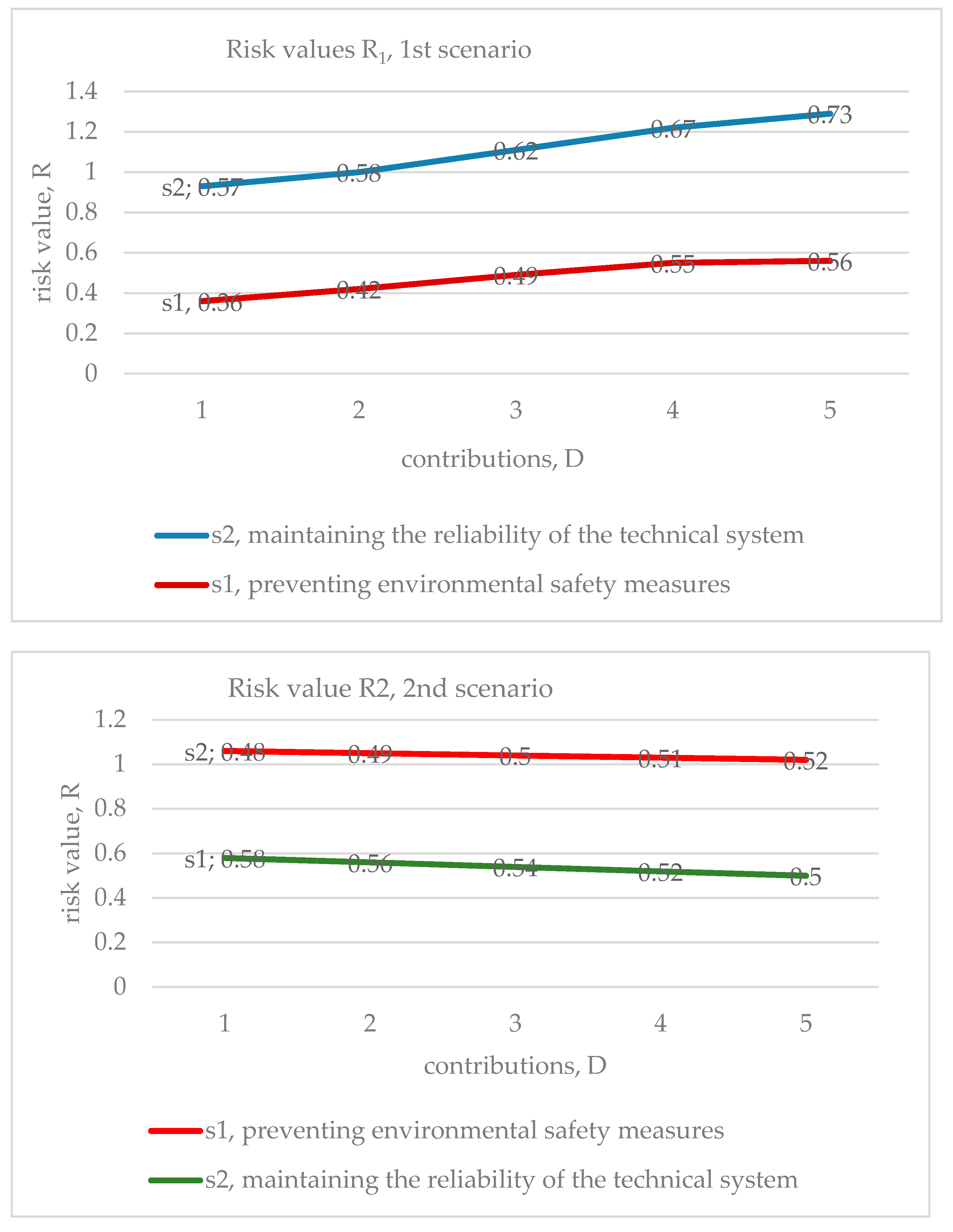
- Each of the four risk curves (four scenarios) presented in Figure 3 (Results of the estimated example for the objective function) is divided into two components. The new ensemble of risk curves has eight segments (second-level scenarios with five micro-scenarios). Information about them is analyzed in Table A1 and Table A2 and on the next four graphs. Table A1 shows that each scenario includes two types of contributions: (1) preventive environmental safety measures, s1, and (2) maintaining the reliability of the technical system, s2. The numerical values make it clear which type is prioritized in the total investment in a particular scenario. The columns indicate the values of risks specific to each of the five micro-scenarios. Further, to assess a specific share of investments (s1 or s2), the set of risk values in the rows is indicated. The following rows have the same information in percentages. A summary of each scenario is presented in the last lines. Table A1 introduces the data for the pessimistic scenario. Table A2 reflects information for an optimistic (one might say, optimal) option.
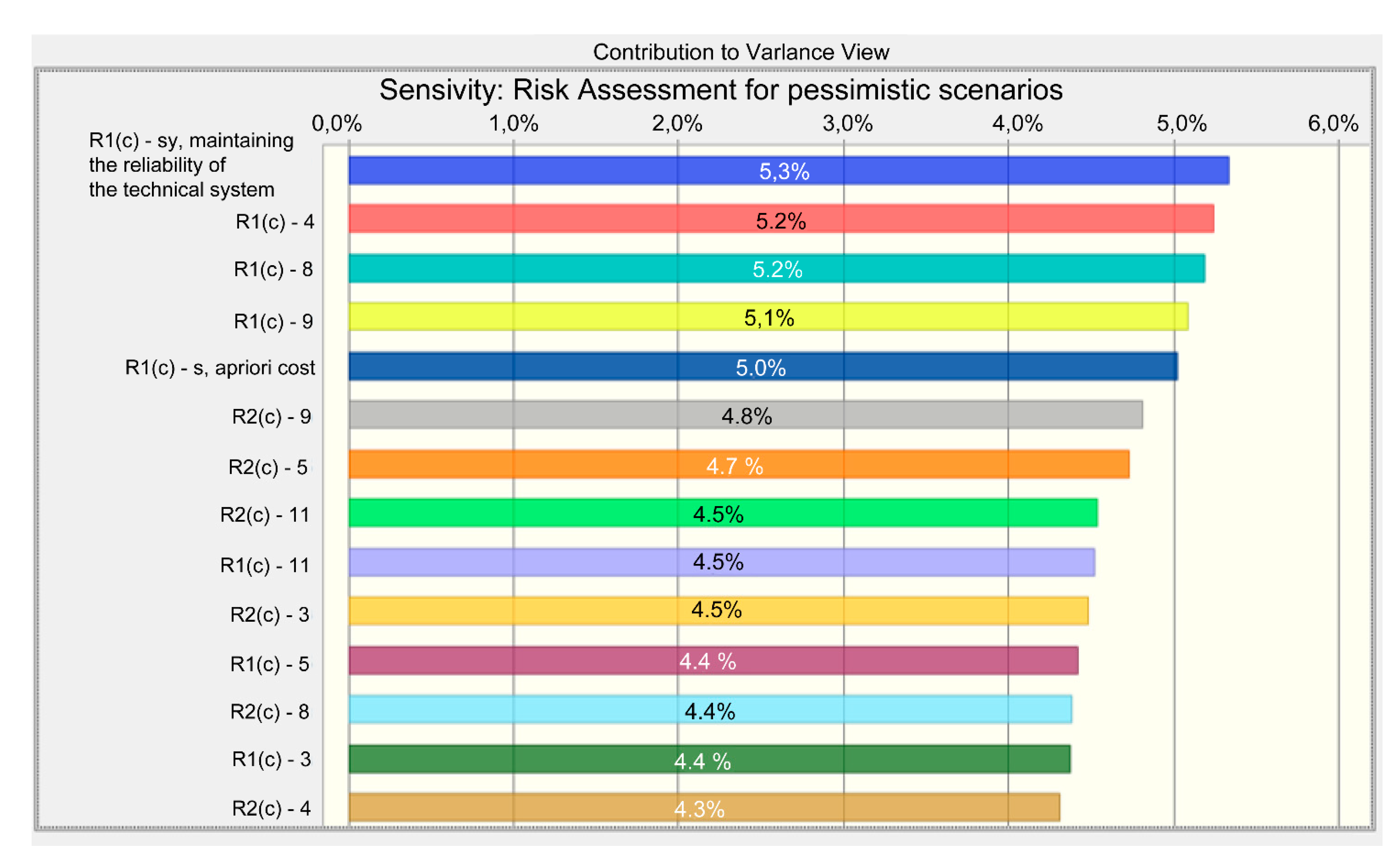
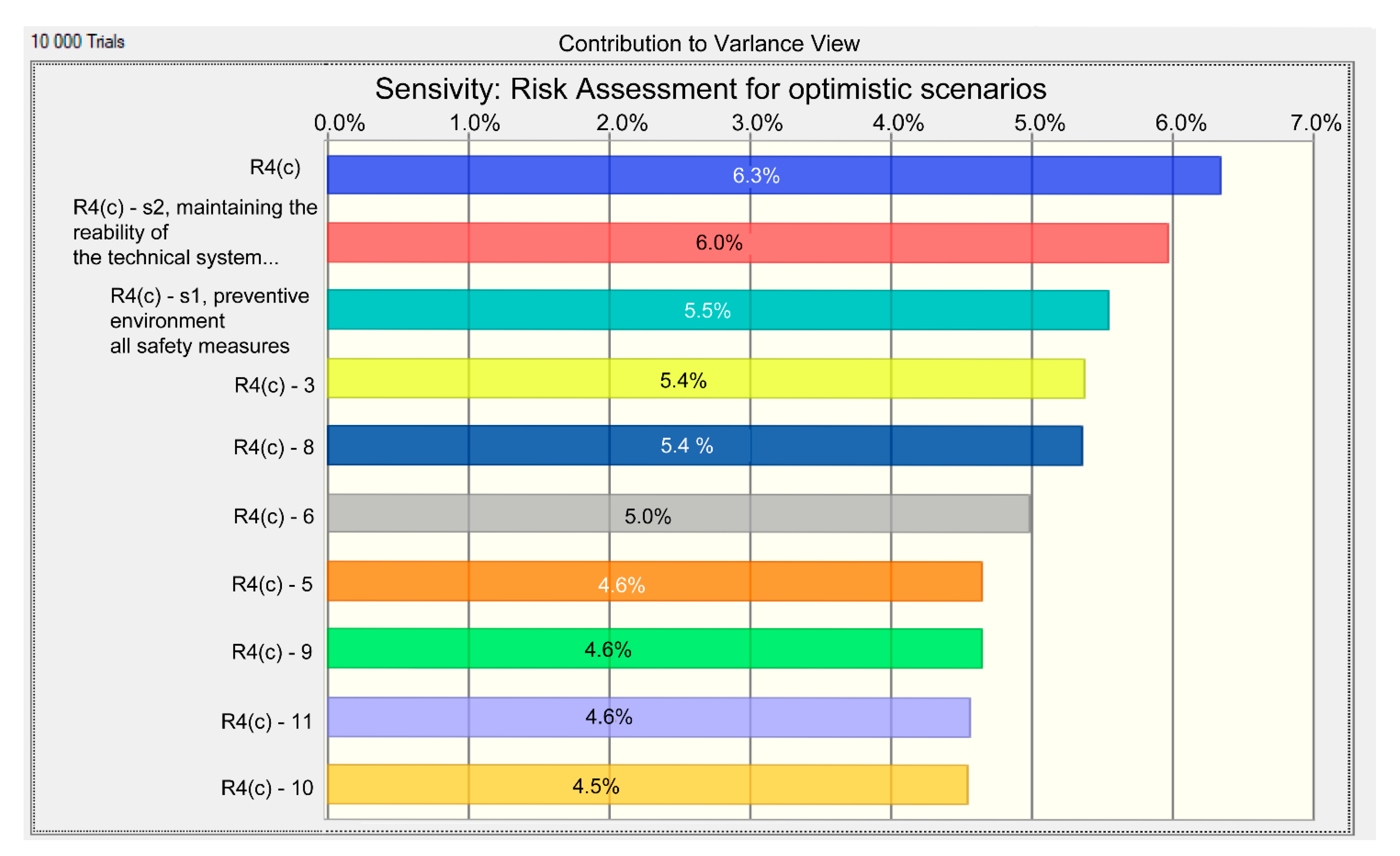
- The authors aimed to identify important relationships between observations, model inputs, and predictions, and to develop a better scenario model. Sensitivity analysis for pessimistic options shows the importance of the s2 parameter. It is wise to focus on the first 10 parameters to control them and simplify the model by relegating other micro-scenarios to the background. It makes sense to address model inputs that do not affect the output or to identify redundant parts of the model structure. It is natural to reduce uncertainty by identifying the input data of the scenario model, which causes significant uncertainty in the output and, therefore, should be focused on increasing the stability of the forecast. Additionally, the most essential initial variables and their changes should be controlled first. Based on the results obtained, it can be concluded that fluctuations in the value of risk when only one scenario variable is changed are rather small; therefore, the forecast risk associated with this variable is low. As a result of the calculation, the risk sensitivity of the optimistic scenarios was determined. The sensitivity diagram shows that s2 and s1 are the key scenario parameters that determine the construction projects’ degree of risk. Therefore, it is important to control them in order to improve the environmental safety of projects. It can also be concluded that in pessimistic and optimistic scenarios, the s2 parameter is a priority contribution to improving environmental safety in the construction industry.
Appendix B. Figures and Tables


| R1(c), p = 0.3 | ∑ R1(c) | ∑ R1(c), % | |||||
| preventive environmental safety measures, s1 | 0.36 | 0.42 | 0.49 | 0.55 | 0.56 | 2.38 | 42.88% |
| maintaining the reliability of the technical system, s2 | 0.57 | 0.58 | 0.62 | 0.67 | 0.73 | 3.17 | 57.12% |
| ∑ R1(c) | 0.93 | 1.0 | 1.11 | 1.22 | 1.29 | 5.55 | 100% |
| R2(c), p = 0.6 | ∑ R2(c) | ∑ R2(c), % | |||||
| preventive environmental safety measures, s1 | 0.58 | 0.56 | 0.54 | 0.52 | 0.5 | 2.7 | 51.92% |
| maintaining the reliability of the technical system, s2 | 0.48 | 0.49 | 0.5 | 0.51 | 0.52 | 2.5 | 48.08% |
| ∑ R2(c) | 1.06 | 1.05 | 1.04 | 1.03 | 1.02 | 5.2 | 100% |
| R3(c), p = 0.1 | ∑ R3(c) | ∑ R3(c), % | |||||
| preventive environmental safety measures, s1 | 0.18 | 0.27 | 0.35 | 0.44 | 0.52 | 1.76 | 31.71% |
| maintaining the reliability of the technical system, s2 | 0.61 | 0.69 | 0.78 | 0.86 | 0.95 | 3.89 | 70.09% |
| ∑ R3(c) | 0.79 | 0.96 | 1.13 | 1.3 | 1.47 | 5.65 | 100% |
| R4(c), p = 0.7 | ∑ R4(c) | ∑ R4(c), % | |||||
| preventive environmental safety measures, s1 | 0.66 | 0.62 | 0.51 | 0.47 | 0.43 | 2.69 | 51.73% |
| maintaining the reliability of the technical system, s2 | 0.39 | 0.35 | 0.34 | 0.34 | 0.3 | 1.72 | 33.08% |
| ∑ R4(c) | 1.05 | 0.97 | 0.85 | 0.81 | 0.73 | 4.41 | 100% |


References
- Kuang, Z.; Gu, Y.; Rao, Y.; Huang, H. Biological risk assessment of heavy metals in sediments and health risk assessment in marine organisms from Daya Bay, China. J. Mar. Sci. Eng. 2020, 9, 17. [Google Scholar] [CrossRef]
- Pirsaheb, M.; Hadei, M.; Sharafi, K. Human health risk assessment by Monte Carlo simulation method for heavy metals of commonly consumed cereals in Iran: Uncertainty and sensitivity analysis. J. Food Compos. Anal. 2021, 96, 103697. [Google Scholar] [CrossRef]
- Von Neumann, J. Various techniques used in connection with random digits. Natl. Bur. Stand. Appl. Math. Ser. 1951, 12, 36–38. [Google Scholar]
- Peres, Y. Iterating von Neumann’s procedure for extracting random bits. Ann. Stat. 1992, 20, 590–597. [Google Scholar] [CrossRef]
- Metropolis, N. The beginning of the Monte Carlo method. Los Alamos Sci. 1987, 15, 125–130. [Google Scholar]
- Metropolis, N.; Ulam, S. The Monte Carlo method. J. Am. Stat. Assoc. 1949, 44, 335–341. [Google Scholar] [CrossRef] [PubMed]
- Gardiner, V.; Lazarus, R.; Metropolis, N.; Ulam, S. On certain sequences of integers defined by sieves. Math. Mag. 1956, 29, 117. [Google Scholar] [CrossRef][Green Version]
- Smith, R.L. Use of Monte Carlo simulation for human exposure assessment at a superfund site. Risk Anal. 1994, 14, 433–439. [Google Scholar] [CrossRef] [PubMed]
- Sonnemann, G.; Castells, F.; Schuhmacher, M.; Hauschild, M. Integrated Life-Cycle and Risk Assessment for Industrial Processes; CRC Press: Boca Raton, FL, USA, 2004; 391p. [Google Scholar] [CrossRef]
- Rosa, E.A. Metatheoretical foundations for post-normal risk. J. Risk Res. 1998, 1, 15–44. [Google Scholar] [CrossRef]
- Renn, O.; Klinke, A. Risk governance and resilience: New approaches to cope with uncertainty and ambiguity. In Risk Governance: The Articulation of Hazard, Politics and Ecology; Paleo, U., Ed.; Springer: Dordrecht, The Netherlands, 2015; pp. 19–41. [Google Scholar]
- Campbell, S. Determining overall risk. J. Risk Res. 2005, 8, 569–581. [Google Scholar] [CrossRef]
- Wiener, J.B.; Graham, J.D. Resolving risk tradeoffs. In Risk versus Risk: Tradeoffs in Protecting Health and the Environment; Graham, J.D., Wiener, J.B., Sunstein, C.R., Eds.; Harvard University Press: Cambridge, MA, USA, 1997; pp. 226–272. [Google Scholar] [CrossRef]
- Lowrance, W.W. Of Acceptable Risk: Science and the Determination of Safety; W. Kaufmann: Los Altos, CA, USA, 1976; 180p. [Google Scholar]
- Kaplan, S.; Garrick, B.J. On the quantitative definition of risk. Risk Anal. 1981, 1, 11–27. [Google Scholar] [CrossRef]
- Fathi-Vajargah, B.; Hassanzadeh, Z. A new Monte Carlo method for solving systems of linear algebraic equations. Comput. Methods Differ. Equ. 2021, 9, 159–179. [Google Scholar]
- Wang, M.-J.; Sjoden, G.E. Experimental and computational dose rate evaluation using SN and Monte Carlo method for a packaged 241AmBe neutron source. Nucl. Sci. Eng. 2021, 195, 1154–1175. [Google Scholar] [CrossRef]
- Chapra, S.C. Applied Numerical Methods with MATLAB for Engineers and Scientists; McGraw-Hill Education: New York, NY, USA, 2018; 697p. [Google Scholar]
- Kushner, H.J.; Dupuis, P.G. Numerical Methods for Stochastic Control Problems in Continuous Time—Applications of Mathematics; Springer: New York, NY, USA, 2014; 475p. [Google Scholar]
- Branford, S.; Sahin, C.; Thandavan, A.; Weihrauch, C.; Alexandrov, V.; Dimov, I. Monte Carlo methods for matrix computations on the grid. Futur. Gener. Comput. Syst. 2008, 24, 605–612. [Google Scholar] [CrossRef]
- Rashki, M. The soft Monte Carlo method. Appl. Math. Model. 2021, 94, 558–575. [Google Scholar] [CrossRef]
- Løvbak, E.; Samaey, G.; Vandewalle, S. A multilevel Monte Carlo method for asymptotic-preserving particle schemes in the diffusive limit. Numer. Math. 2021, 148, 141–186. [Google Scholar] [CrossRef]
- Peter, R.; Bifano, L.; Fischerauer, G. Monte Carlo method for the reduction of measurement errors in the material parameter estimation with cavities. Tech. Mess. 2021, 88, 303–310. [Google Scholar] [CrossRef]
- Chen, G.; Wan, Y.; Lin, H.; Hu, H.; Liu, G.; Peng, Y. Vertical tank capacity measurement based on Monte Carlo method. PLoS ONE 2021, 16, e0250207. [Google Scholar] [CrossRef]
- Huo, X. A compact Monte Carlo method for the calculation of k∞ and its application in analysis of (n,xn) reactions. Nucl. Eng. Des. 2021, 376, 111092. [Google Scholar] [CrossRef]
- Choobar, B.G.; Modarress, H.; Halladj, R.; Amjad-Iranagh, S. Electrodeposition of lithium metal on lithium anode surface, a simulation study by: Kinetic Monte Carlo-embedded atom method. Comput. Mater. Sci. 2021, 192, 110343. [Google Scholar] [CrossRef]
- Sharma, A.; Sastri, O.S.K.S. Numerical solution of Schrodinger equation for rotating Morse potential using matrix methods with Fourier sine basis and optimization using variational Monte-Carlo approach. Int. J. Quantum Chem. 2021, 121, e26682. [Google Scholar] [CrossRef]
- Toropov, A.; Toropova, A.; Lombardo, A.; Roncaglioni, A.; Lavado, G.; Benfenati, E. The Monte Carlo method to build up models of the hydrolysis half-lives of organic compounds. SAR QSAR Environ. Res. 2021, 32, 463–471. [Google Scholar] [CrossRef] [PubMed]
- Che, Y.; Wu, X.; Pastore, G.; Li, W.; Shirvan, K. Application of Kriging and Variational Bayesian Monte Carlo method for improved prediction of doped UO2 fission gas release. Ann. Nucl. Energy 2021, 153, 108046. [Google Scholar] [CrossRef]
- Pitchai, P.; Jha, N.K.; Nair, R.G.; Guruprasad, P. A coupled framework of variational asymptotic method based homogenization technique and Monte Carlo approach for the uncertainty and sensitivity analysis of unidirectional composites. Compos. Struct. 2021, 263, 113656. [Google Scholar] [CrossRef]
- Toropova, A.P.; Toropov, A.A. Can the Monte Carlo method predict the toxicity of binary mixtures? Environ. Sci. Pollut. Res. 2021, 28, 39493–39500. [Google Scholar] [CrossRef]
- Lee, E.-K. Determination of burnup limit for CANDU 6 fuel using Monte-Carlo method. Nucl. Eng. Technol. 2021, 53, 901–910. [Google Scholar] [CrossRef]
- Oh, K.-Y.; Nam, W. A fast Monte-Carlo method to predict failure probability of offshore wind turbine caused by stochastic variations in soil. Ocean Eng. 2021, 223, 108635. [Google Scholar] [CrossRef]
- Oliver, J.; Qin, X.S.; Madsen, H.; Rautela, P.; Joshi, G.C.; Jorgensen, G. A probabilistic risk modelling chain for analysis of regional flood events. Stoch. Environ. Res. Risk Assess. 2019, 33, 1057–1074. [Google Scholar] [CrossRef]
- Stewart, M.G.; Ginger, J.D.; Henderson, D.J.; Ryan, P.C. Fragility and climate impact assessment of contemporary housing roof sheeting failure due to extreme wind. Eng. Struct. 2018, 171, 464–475. [Google Scholar] [CrossRef]
- Qin, H.; Stewart, M.G. Risk perceptions and economic incentives for mitigating windstorm damage to housing. Civ. Eng. Environ. Syst. 2020, 38, 1–19. [Google Scholar] [CrossRef]
- Malmasi, S.; Fam, I.M.; Mohebbi, N. Health, safety and environment risk assessment in gas pipelines. J. Sci. Ind. Res. 2010, 69, 662–666. [Google Scholar]
- Karagöz, D. Asymmetric control limits for range chart with simple robust estimator under the non-normal distributed process. Math. Sci. 2018, 12, 249–262. [Google Scholar] [CrossRef]
- Couto, P.R.G.; Carreteiro, J.; de Oliveir, S.P. Monte Carlo simulations applied to uncertainty in measurement. In Theory and Applications of Monte Carlo Simulations; Chan, V., Ed.; InTechOpen: London, UK, 2013; pp. 27–51. [Google Scholar]
- Kalos, M.H.; Whitlock, P.A. Monte Carlo Methods; Wiley-VCH: Weinheim, Germany, 2009; 203p. [Google Scholar]
- Bieda, B. Stochastic approach to municipal solid waste landfill life based on the contaminant transit time modeling using the Monte Carlo (MC) simulation. Sci. Total Environ. 2013, 442, 489–496. [Google Scholar] [CrossRef] [PubMed]
- Aczel, A.D. Statistics: Concepts and Applications; Irwin: Chicago, IL, USA, 1995; 533p. [Google Scholar]
- Benjamin, J.R.; Cornell, C.A. Probability, Statistics and Decision for Civil Engineers; Dover Publication: Mineola, NY, USA, 2018; 684p. [Google Scholar]
- Bieda, B. Stochastic Analysis in Production Process and Ecology under Uncertainty; Springer: Berlin/Heidelberg, Germany; New York, NY, USA, 2012; 189p. [Google Scholar]
- Taleb, N.N. The Black Swan: The Impact of the Highly Improbable; Random House: New York, NY, USA, 2007; 366p. [Google Scholar]
- Strakhova, N.A.; Karmazin, S.A. Characteristics of the most used methods of risk analysis. Eurasian Sci. J. 2013, 3, 122–128. Available online: http://naukovedenie.ru/PDF/22ergsu313.pdf (accessed on 24 November 2021).
- Jones, M.; Silberzahn, P. Constructing Cassandra: Reframing Intelligence Failure at the CIA, 1947–2001; Stanford University Press: Stanford, CA, USA, 2020; 375p. [Google Scholar]
- Larionov, A.; Nezhnikova, E. Energy efficiency and the quality of housing projects. ARPN J. Eng. Appl. Sci. 2016, 11, 2023–2029. [Google Scholar]
- Smirnova, E.; Larionov, A. Justification of environmental safety criteria in the context of sustainable development of the construction sector. E3S Web Conf. 2020, 157, 06011. [Google Scholar] [CrossRef]
- Larionova, Y.; Smirnova, E. Substantiation of ecological safety criteria in construction industry, and housing and communal services. IOP Conf. Ser. Earth Environ. Sci. 2020, 543, 012002. [Google Scholar] [CrossRef]
- Smirnova, E. Environmental risk analysis in construction under uncertainty. In Reconstruction and Restoration of Architectural Heritage; Sementsov, S., Leontyev, A., Huerta, S., Menéndez Pidal de Nava, I., Eds.; CRC Press: London, UK, 2020; pp. 222–227. [Google Scholar] [CrossRef]
- Kingman, J. Poisson Processes; Oxford Studies in Probability; Clarendon: Oxford, UK, 2002; 104p. [Google Scholar]
- Aven, R. Risk analysis and management: Basic concepts and principles. Reliab. Theory Appl. 2009, 1, 57–73. [Google Scholar]
- Stoica, G. Relevant coherent measures of risk. J. Math. Econ. 2006, 42, 794–806. [Google Scholar] [CrossRef]
- Smirnova, E. Monte Carlo simulation of environmental risks of technogenic impact. In Contemporary Problems of Architecture and Construction; Rybnov, E., Akimov, P., Khalvashi, M., Vardanyan, E., Eds.; CRC Press: London, UK, 2021; pp. 355–360. [Google Scholar] [CrossRef]
- Zadeh, L.A. Fuzzy sets as a basis for a theory of possibility. Fuzzy Sets Syst. 1999, 100, 9–34. [Google Scholar] [CrossRef]
- Pappenberger, F.; Beven, K.J. Ignorance is bliss: Or seven reasons not to use uncertainty analysis. Water Resour. Res. 2006, 42, W05302. [Google Scholar] [CrossRef]
- Silberzahn, P. Welcome to Extremistan: Why Some Things Cannot be Predicted and What That Means for Your Strategy. 2011. Available online: https://silberzahnjones.com/2011/11/10/welcome-to-extremistan/ (accessed on 24 November 2021).
- Spiegelhalter, D.; Pearson, M.; Short, I. Visualizing uncertainty about the future. Science 2011, 333, 1393–1400. [Google Scholar] [CrossRef] [PubMed]
- Semenoglou, A.-A.; Spiliotis, E.; Makridakis, S.; Assimakopoulos, V. Investigating the accuracy of cross-learning time series forecasting methods. Int. J. Forecast. 2021, 37, 1072–1084. [Google Scholar] [CrossRef]
- Dalal, S.R.; Fowlkes, E.B.; Hoadley, B. Risk analysis of the space shuttle: Pre-Challenger prediction of failure. J. Am. Stat. Assoc. 1989, 84, 945–957. [Google Scholar] [CrossRef]
- Kelly, D.L.; Smith, C.L. Risk analysis of the space shuttle: Pre-Challenger Bayesian prediction of failure. In Proceedings of the Conference on NASA Systems Safety Engineering and Risk Management, Los Angeles, CA, USA, 20 February 2008; Office of Nuclear Energy, Science, and Technology/Idaho National Laboratory: Washington, DC, USA, 2008; pp. 1–12. [Google Scholar]
- Portugués, E.G. Notes for Predictive Modeling. Version 5.9.0. 2021. Available online: https://bookdown.org/egarpor/PM-UC3M/ (accessed on 24 November 2021).


| D1 | D2 | D3 | D4 | R1(c) | R2(c) | R3(c) | R4(c) | P1 | P2 | P3 | P4 |
|---|---|---|---|---|---|---|---|---|---|---|---|
| 0 | 0 | 0 | 0 | 0.3 | 0.6 | 0.1 | 0.7 | 0.3 | 0.6 | 0.1 | 0.7 |
| 0.07 | 0.04 | 0.09 | 0.03 | 0.36 | 0.58 | 0.185 | 0.66 | 0.27 | 0.54 | 0.095 | 0.63 |
| 0.14 | 0.08 | 0.18 | 0.06 | 0.42 | 0.56 | 0.27 | 0.62 | 0.24 | 0.48 | 0.09 | 0.56 |
| 0.21 | 0.12 | 0.27 | 0.09 | 0.49 | 0.54 | 0.355 | 0.51 | 0.18 | 0.42 | 0.085 | 0.42 |
| 0.28 | 0.16 | 0.36 | 0.12 | 0.55 | 0.52 | 0.44 | 0.47 | 0.15 | 0.36 | 0.08 | 0.35 |
| 0.35 | 0.2 | 0.45 | 0.15 | 0.56 | 0.5 | 0.525 | 0.43 | 0.12 | 0.3 | 0.075 | 0.28 |
| 0.42 | 0.24 | 0.54 | 0.18 | 0.57 | 0.48 | 0.61 | 0.39 | 0.09 | 0.24 | 0.07 | 0.21 |
| 0.49 | 0.28 | 0.63 | 0.21 | 0.58 | 0.49 | 0.695 | 0.35 | 0.06 | 0.21 | 0.065 | 0.14 |
| 0.56 | 0.32 | 0.72 | 0.24 | 0.62 | 0.5 | 0.78 | 0.345 | 0.045 | 0.18 | 0.06 | 0.105 |
| 0.63 | 0.36 | 0.81 | 0.27 | 0.67 | 0.51 | 0.865 | 0.34 | 0.03 | 0.15 | 0.055 | 0.07 |
| 0.7 | 0.4 | 0.9 | 0.3 | 0.73 | 0.52 | 0.95 | 0.3 | 0 | 0.12 | 0.05 | 0 |
Publisher’s Note: MDPI stays neutral with regard to jurisdictional claims in published maps and institutional affiliations. |
© 2021 by the authors. Licensee MDPI, Basel, Switzerland. This article is an open access article distributed under the terms and conditions of the Creative Commons Attribution (CC BY) license (https://creativecommons.org/licenses/by/4.0/).
Share and Cite
Larionov, A.; Nezhnikova, E.; Smirnova, E. Risk Assessment Models to Improve Environmental Safety in the Field of the Economy and Organization of Construction: A Case Study of Russia. Sustainability 2021, 13, 13539. https://doi.org/10.3390/su132413539
Larionov A, Nezhnikova E, Smirnova E. Risk Assessment Models to Improve Environmental Safety in the Field of the Economy and Organization of Construction: A Case Study of Russia. Sustainability. 2021; 13(24):13539. https://doi.org/10.3390/su132413539
Chicago/Turabian StyleLarionov, Arkadiy, Ekaterina Nezhnikova, and Elena Smirnova. 2021. "Risk Assessment Models to Improve Environmental Safety in the Field of the Economy and Organization of Construction: A Case Study of Russia" Sustainability 13, no. 24: 13539. https://doi.org/10.3390/su132413539
APA StyleLarionov, A., Nezhnikova, E., & Smirnova, E. (2021). Risk Assessment Models to Improve Environmental Safety in the Field of the Economy and Organization of Construction: A Case Study of Russia. Sustainability, 13(24), 13539. https://doi.org/10.3390/su132413539