Control of Laser Scanner Trilateration Networks for Accurate Georeferencing of Caves: Application to El Castillo Cave (Spain)

Abstract

There is a growing demand for measurements of natural and built elements, which require quantifiable accuracy and reliability, within various fields of application. Measurements from 3D Terrestrial Laser Scanner come in a point cloud, and different types of surfaces such as spheres or planes can be modelled. Due to the occlusions and/or limited field of view, it is seldom possible to survey a complete feature from one location, and information has to be acquired from multiple points of view and later co-registered and geo-referenced to obtain a consistent coordinate system. The aim of this paper is not to match point clouds, but to show a methodology to adjust, following the traditional topo-geodetic methods, 3DTLS data by modelling references such as calibrated spheres and checker-boards to generate a 3D trilateration network from them to derive accuracy and reliability measurements and post-adjustment statistical analysis. The method tries to find the function that best fits the measured data, taking into account not only that the measurements made in the field are not perfect, but that each one of them has a different deviation depending on the adjustment of each reference, so they have to be weighted accordingly.

1. Introduction

Caves open to the public constitute an important heritage asset exploited as a tourist resource. In these circumstances, it is the duty of the competent administration and also of all the actors in the tourism industry to ensure the preservation of the assets with their enhancement within the framework of “sustainable tourism” [1].

The cave of El Castillo is included in the World Heritage List, which implies above all a commitment to the responsible and sustainable management of this property, which we should bequeath to future generations in the same state in which it has come down to us from the depths of geological and prehistoric time.

Caves are characterised by a series of particularities from a topographical perspective, such as the lack of lighting, almost constant temperature, high humidity, the existence of small spaces, complex access, the relationship between the interior and the exterior, and so on [1].

Traditionally, goniometers, compasses, theodolites, tachymeters, total stations, and gyroscopic theodolites have been used for mapping, which were linked to data taken with Global Navigation Satellite Systems (GNSS) in the exterior to be georeferenced [2].

Traditional topographic methods are based on closed polygon or link traverses, but it is when redundant data are measured that accuracy is improved and overall measurements can be reliably controlled. The number of excess observations is called redundancies or degrees of freedom. Several solutions can be given to the question posed, but the one that satisfies the set of mathematical relationships between the measured quantities and also minimises the sum of squares of the residuals (i.e., the least squares solution) will be sought.

The least squares adjustment computations are essential when you want to carry out a work of topography, geodesy, or in general geomatics, offering the maximum reliability and above all accuracy [3] in caves. Geodetic networks and their design [4] have been widely investigated since the beginning [5,6]. Since then, several works were described in papers published in scientific journals (see e.g., [7,8,9,10,11,12,13,14,15,16]).

Three-Dimensional Terrestrial Laser Scanners (3DTLS) can capture a large number of measurements rapidly, with high precision and spatial resolution. Nowadays, in order to get the scans into a consistent coordinate system, they have to be registered, and rigid solid transformations are performed. Point clouds are usually registered using the Iterative Closest Points (ICP) algorithm proposed by Besl [17], but this does not provide explicit information about their in-depth geometric qualities [18]; it defines a spatial similarity transformation embedded in a Gauss–Helmert model [19] to estimate the variances of the unit weight and standard deviations of the combined data sets.

The purpose of this paper is not to create a method for co-registering and georeferencing point clouds, but to extract observations to create a 3D trilateration network to be processed in the way of traditional geodetic networks in order to derive accuracy and reliability measurements and post-adjustment statistical analysis.

This paper shows how to use 3DTLS as a metrological tool to perform least-squares adjustment of linked networks inside caves and to derive error enclosures for the whole working area. First, spheres and planes are adjusted from each 3DTLS station and weighted according to their accuracy to generate the average values to be used as sides of a 3D trilateration which is then adjusted by means of a least squares adjustment.

In order to have reference points to adjust the information, it is necessary to model the information of the point cloud, in which different types of surfaces (spheres or planes) are adjusted to a subset of the point cloud and the accuracy and reliability of the data obtained will be assessed according to the distances and resolution at which it is obtained. When adjusting networks, one must first know the instrument with which the observations will be made, given that there are different types of 3DTLS.

2. Materials and Methods

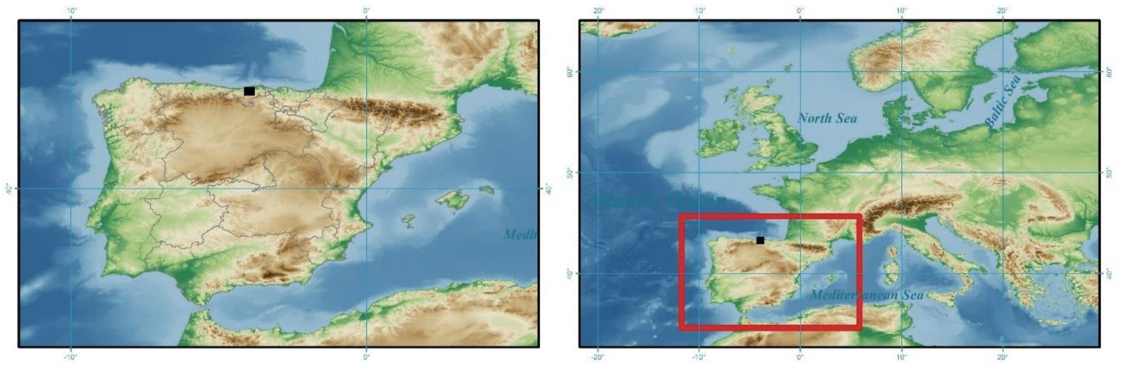
2.1. Study Area

Monte Castillo is a mountain in the Dobra mountain range, within the municipality of Puente Viesgo, in Cantabria, Spain (Figure 1). It is well known for the number of caves with cave art it houses. It has a conical limestone structure in which nearly 200 cavities have been recorded. Of these, four caves with Palaeolithic cave art were declared World Heritage Sites by UNESCO in 2008.

One of the essential aspects in the management of caves with rock art is the maintenance of equilibrium (or a balance) in the environmental conditions of the subterranean space [20]. The reason for the conservation of this heritage from some 40,000 years ago to the present day is the preservation of conditions of marked stability, which are favoured by the absolute or relative isolation of this subterranean environment.

Thanks to the new method, it has been possible to determine the relationship between the cavities that make up the karst, favouring the sustainability and conservation of the World Heritage caves.

As shown, least squares adjustments from 3DTLS targets can help not only to obtain better cartography but to understand the complexity of the karst.

Having an accurate cartographic base is important when geo-referencing features, but it is even more important when parameters are interrelated and used to develop and test knowledge-based prediction models such as hydrochemical, microbiological, climatic, geotechnical, or faunal models which require measuring multiple parameters, many of which are highly correlated [1].

From its discovery in the early 20th century, El Castillo Cave has had several cartographies (Figure 2) that have been used to record data along time.

2.2. Overall Workflow

The overall workflow of the proposed method is shown in Figure 3. It basically consists of three parts. The first part deals with the field data collection; the second part deals with standard processing to obtain target and spheres adjusted models and fixed coordinates points; and the third part deals with least squares processing, measures of accuracy and post-adjustment statistical analysis of the 3D trilateration network.

The field work for data acquisition took place in 2015. The 3DTLS used to record data was FARO Focus X330 [24].

2.3. Propagation and Accuracy of Random Errors in Indirectly Measured Quantities

2.3.1. Introduction

When making an adjustment, it is important to know the estimated errors in both the adjusted observations and the derived quantities. Error propagation expressions for indirectly measured quantities will be shown below.

2.3.2. Basic Error Propagation Equation

Sometimes unknown values are determined indirectly by making direct measurements of other quantities functionally related to the desired unknowns. This is the case for the distances of the 3D laser scanner trilateration network, where the positions of the spheres are determined from the point cloud, and distances between them are derived to produce the trilateration network. Since all directly measured quantities contain an error, any calculated values derived from them will contain errors. This intrusion, or propagation of errors, that happens with quantities calculated from direct measurements is called error propagation and is one of the most important aspects when compensating 3D laser scanner networks.

In the following, it will be assumed that the systematic errors have been eliminated, so that only the random errors in the direct observations remain. To derive the expressions, two independently observed quantities, $x_1$ and $x_2$, will be considered with a standard error ${\mathrm{\sigma }}_1$ and ${\mathrm{\sigma }}_2$ and constants $a_1$ and $a_2.$ Since $x_1$ and $x_2$ are two independently observed quantities, each has a different probability density function. The errors in n determinations of $x_1$ will be taken to be ${\epsilon }_1^i,{\epsilon }_1^{ii},\dots ,{\epsilon }_1^n$, and the errors in n determinations of $x_2$ will be ${\epsilon }_2^i,{\epsilon }_2^{ii},\dots ,{\epsilon }_2^n$; therefore $z_T$, the true value of z for each independent measurement will be:

$$Z_T=\left[\begin{array}{c}{a}_1\cdot \left(x_1^i-{\epsilon }_1^i\right) + a_2\left(x_2^i-{\epsilon }_2^i\right) =a_1\cdot x_1^i+a_2\cdot x_2^i-\left(a_1\cdot {\epsilon }_1^i+a_2\cdot {\epsilon }_2^i\right)\\ a_1\left(x_1^{ii}-{\epsilon }_1^{ii}\right) + a_2\left(x_2^{ii}-{\epsilon }_2^{ii}\right) =a_1\cdot x_1^{ii}+a_2\cdot x_2^{ii}-\left(a_1\cdot {\epsilon }_1^{ii}+a_2\cdot {\epsilon }_2^{ii}\right)\\ a_1\left(x_1^{iii}-{\epsilon }_1^{iii}\right) + a_2\left(x_2^{iii}-{\epsilon }_2^{iii}\right) =a_1\cdot x_1^{iii}+a_2\cdot x_2^{iii}-\left(a_1\cdot {\epsilon }_1^{iii}+a_2\cdot {\epsilon }_2^{iii}\right)\end{array}\right]$$

(1)

There are multiple references ([25,26,27,28], etc.) that describe the process up to the expression of the general law of propagation of variances for linear or non-linear equations:

$${\Sigma }_{zz}=A\cdot \Sigma \cdot A^T$$

(2)

where ${\Sigma }_{zz}$ is the covariance matrix for the function Z. For a set of non-linear equations linearised following Taylor’s theorem, the coefficient matrix A is called the Jacobian matrix, which is a matrix of partial derivatives regarding each unknown.

If the measures $x_1,x_2,\dots ,x_n$ are disjoint (i.e., statistically independent), the covariance terms ${\mathrm{\sigma }}_{x_1{x}_2},{\mathrm{\sigma }}_{x_1{x}_3}$,… are equal to zero. The law of variance propagation governs how errors from statistically independent measurements propagate in a function.

2.3.3. Accuracy of Indirectly Determined Quantities

From a fit, it is important to know the estimated errors in both the fitted observations and the derived quantities. The propagation expressions for the calculated values in the least square solution are shown below.

Development of the Covariance Matrix

If a fit involving weighted observations is considered as is the case, the matrix form for the systems of weighted observation equations is:

$$PAX=PL+PV$$

(3)

and the least square solution of the weighted equations is given by:

$$X={\left(A^{T}PA\right)}^{-1}{A}^{T}PL$$

(4)

X contains the most probable values of the unknowns, if we consider $X_v$ as the true value, it will differ from X by a small amount $∆X$, such that:

$$X+∆X=X_v$$

(5)

Hence, $∆X$ represents the errors of the fitted values.

Since the weight of an observation is inversely proportional to its variance, the variance of an observation of weight p can be expressed in terms of variance as:

$$s_i^2=\frac{s_0^2}{p_i}$$

(6)

and operating, we can reach:

$$s_x^2=s_0^2{\left(A^{T}PA\right)}^{-1}=s_0^2{N}^{-1}=s_0^2{Q}_{xx}$$

(7)

In least square fits, the matrix $Q_{xx}$ is known as the variance-covariance matrix, or simply the covariance matrix. The diagonal elements of the matrix when multiplied by $S_0^2$ give variances of the fitted quantities, the off-diagonal elements multiplied by $S_0^2$ give variances of the fitted quantities, and the off-diagonal elements multiplied by $S_0^2$ give the covariances. From the above expression, the estimated standard deviation for any unknown parameter calculated from a system of observation equations is expressed as:

$$s_i=s_0\sqrt{q_{x_i{x}_i}}$$

(8)

where $q_{x_i{x}_i}$ is the diagonal element (of the i-th row and columns) of the matrix $Q_{xx}$, which, as denoted above, is equal to the inverse of the matrix of normal equations. Since the matrix of normal equations is symmetric, its inverse is also symmetric, and therefore the covariance matrix is a symmetric matrix.

Standard Deviation of the Calculated Quantities

Considering the law of variance propagation:

$${\Sigma }_{ll}=A{\displaystyle \sum }_{xx}{A}^T$$

(9)

where $\widehat{l}$ represents the fitted observations, ${\Sigma }_{\widehat{l}\widehat{l}}$ the covariance matrix of the fitted observations, ${\Sigma }_{xx}$ the covariance matrix of the unknown parameters, and A the coefficient matrix. Rearranging the matrix and applying the above expressions, we arrive at the standard deviations of the fitted observations:

$${\Sigma }_{ll}^2={\mathrm{s}}_l^2=A{\Sigma }_{xx}{A}^T=A{s}_0^2{\left(A^{T}WA\right)}^{-1}{A}^T=s_0^{2}A{Q}_{xx}{A}^T=s_0^2{Q}_{ll}$$

(10)

where $A{Q}_{xx}{A}^T=Q_{ll}$, which is known as the covariance matrix of the fitted observations.

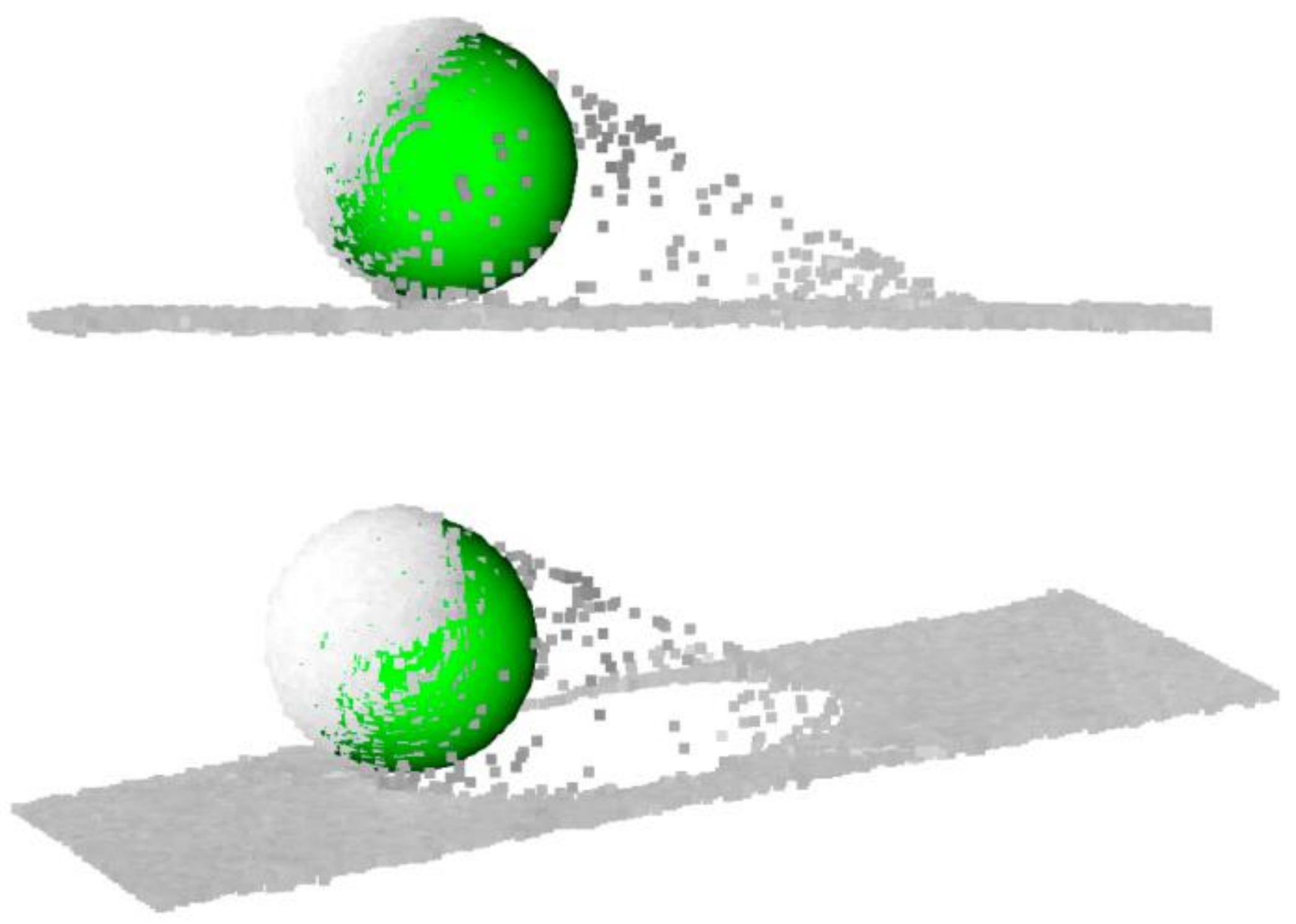
2.3.4. Fitting Spherical Objects from Point Clouds

Model fitting can be presented as an optimisation problem, where we look for those parameters of a model type that lead to the best consensus between the selected points and the resulting model. This consensus for a point can be valued as its distance from the model surface, while for the point cloud, it can be measured as the sum of a function of the distances for all points. A low value of this sum indicates a high degree of fit and vice versa. Normally, two distances are used, the algebraic and the geometric. Mathematically, the fit model can be formulated as follows [29,30,31]:

$$mi{n}_{{\mathsf{\tau }}_1,{\mathsf{\tau }}_2,\dots ,{\mathsf{\tau }}_m{{\displaystyle \sum }}_{i=1}^N\mathsf{\Gamma }\left(\mathsf{\Psi }\left[p_i,\mathsf{\Gamma }\left({\mathsf{\tau }}_1,{\mathsf{\tau }}_2,\dots ,{\mathsf{\tau }}_m\right)\right]\right)}$$

(11)

where $\mathsf{\Gamma }\left({\mathsf{\tau }}_1,{\mathsf{\tau }}_2,\dots ,{\mathsf{\tau }}_m\right)$ is the model fit to the point cloud consisting of n points $p_1,p_2,\dots ,p_n$. The model is parametrised by the form m and presents the parameters ${\mathsf{\tau }}_1,{\mathsf{\tau }}_2,\dots ,{\mathsf{\tau }}_m$. $\mathsf{\Psi }$ is a function

2.4. Fitting Spherical Objects from Point Clouds

2.4.1. Problem Definition

Model fitting can be presented as an optimisation problem, where we look for those parameters of a model type that lead to the best consensus between the selected points and the resulting model. This consensus for a point can be valued as its distance from the model surface, while for the point cloud, it can be measured as the sum of a function of the distances for all points. A low value of this sum indicates a high degree of fit and vice versa. Normally, two distances are used, the algebraic and the geometric. Mathematically, the fit model can be formulated:

$$mi{n}_{{\mathsf{\tau }}_1,{\mathsf{\tau }}_2,\dots ,{\mathsf{\tau }}_m}{\displaystyle \sum }_{i=1}^N\mathsf{\Gamma }\left(\mathsf{\Psi }\left[p_i,\mathsf{\Gamma }\left({\mathsf{\tau }}_1,{\mathsf{\tau }}_2,\dots ,{\mathsf{\tau }}_m\right)\right]\right)$$

(12)

where $\mathsf{\Gamma }\left({\mathsf{\tau }}_1,{\mathsf{\tau }}_2,\dots ,{\mathsf{\tau }}_m\right)$ is the model fit to the point cloud consisting of n points $p_1,p_2,\dots ,p_n$. The model is parametrised by the form m and presents the parameters ${\mathsf{\tau }}_1,{\mathsf{\tau }}_2,\dots ,{\mathsf{\tau }}_m$. $\mathsf{\Psi }$ is a function giving the distance (algebraic, orthogonal, or some other measure of distance) from the i-th point $p_i$ of the model, and $\mathsf{\Gamma }$ is a function of this distance (for the least square distance, for the estimator, etc.).

Comparisons between the modelled objects and the point clouds are made following the orthogonal distance as the value of $\mathsf{\Psi }$. For $\mathsf{\Gamma }$, we will use the squared orthogonal distance, converting the previous problem to the following least squares problem:

$$mi{n}_{{\mathsf{\tau }}_1,{\mathsf{\tau }}_2,\dots ,{\mathsf{\tau }}_m}{\displaystyle \sum }_{i=1}^N{\mathsf{\Psi }}^2\left[p_i,\mathsf{\Gamma }\left({\mathsf{\tau }}_1,{\mathsf{\tau }}_2,\dots ,{\mathsf{\tau }}_m\right)\right]$$

(13)

2.4.2. Method of Adjustment

The above problem can be solved with one of the non-linear least squares methods. The Levenberg–Marquard method is usually used since it has better convergence properties if the step given by Newton’s method and the steepest descent method are adaptively combined [29,32].

From the initial estimate of the model parameters ${\mathsf{\Gamma }}_0$, each iteration yields a fit $∆\mathsf{\Gamma }$ given by:

$$∆\mathsf{\Gamma }={\left(J^{T}WJ+\mathrm{\lambda }I\right)}^{-1}\left(J^{T}WD\right)$$

(14)

$${\mathsf{\Gamma }}_1={\mathsf{\Gamma }}_0-∆$$

(15)

where J is the Jacobian matrix, and D is the distance vector given by:

$$J_{ik}=\frac{\partial {\mathsf{\Psi }}_i}{\partial {\mathsf{\tau }}_k}=\frac{\partial \mathsf{\Psi }\left(p_i,{\mathsf{\Gamma }}_0\right)}{\partial {\mathsf{\tau }}_k}$$

(16)

$$D_i=\mathsf{\Psi }\left(p_i,{\mathsf{\Gamma }}_0\right)$$

(17)

W is the weights matrix giving the quality of the measurement of each point, and $\mathrm{\lambda }$ is the Levenberg–Marquardt parameter. For $\mathrm{\lambda }=0$, the Newton step is taken. According to $\mathrm{\lambda }\to \infty$, the iteration offers smaller corrections. The typical adaptive selection process of $\mathrm{\lambda }$ can be found in chapter 15.5 of [14].

The covariance matrix C of the estimated parameters is calculated as:

$$C={\left(J^{T}WJ\right)}^{-1}$$

(18)

According to [33], in the above expressions, it is possible to employ different measures of distance ‘L between the 3D point and the model being fitted. Two commonly employed distances are the algebraic distance and the orthogonal or geometric distance.

Algebraic distance: This measure of distance is defined only by those surfaces that can be expressed in terms of the distance between the 3D point and the model it fits.

This distance measure is defined only by those surfaces that can be expressed as an implicit function. The initial set of the implicit function gives the model surface, for example, $f\left(x,y,z\right)=0$. For any point on the model surface, the implicit function is zero. For any point outside the surface, $f\left(p_{0x},p_{0y},p_{0z}\right)=0$. The value of the implicit function $p_0=\left(p_{0x},p_{0y},p_{0z}\right)$ is related to the distance, although this relation depends on the type of surface. In the case of a sphere of radius r and centred at $c=\left(c_x,c_y,c_z\right)$, the algebraic distance that equals the value of the implicit function is given by $d_{algebraic}={\left(p_{0x}-c_x\right)}^2+{\left(p_{0y}-c_y\right)}^2+{\left(p_{0z}-c_z\right)}^2-r^2$, while the orthogonal or geometric distance from this point to the sphere would be $d_{geometric}=\sqrt{{\left(p_{0x}-c_x\right)}^2+{\left(p_{0y}-c_y\right)}^2+{\left(p_{0z}-c_z\right)}^2}-r$.

This means there is no linear relationship between the algebraic and geometric distance. Approximately the algebraic distance is equal to the square of the geometric distance. This quadratic relationship makes the algebraic distance more sensitive to outliers and noise than the geometric distance.

The algebraic distance has two very attractive elements. First, its calculation is very simple given an implicit functional model of the model. Second, the implicit function formulation provides a result in a linear least squares problem with a non-iterative solution. Therefore, this distance can be a quick way to compute the approximate values.

Geometric distance: This is the smallest distance from a point to the surface of the model, so that the normal to the local surface and the line joining it to the nearest object are collinear. Usually the calculation of the orthogonal distance is more complicated than the calculation of the algebraic distance. In contrast to the algebraic distance which is defined only for those surfaces that can be expressed as an implicit function, the geometric distance can be defined for all surfaces. When a least squares estimation is used, the geometric distance is always a non-linear (sometimes constrained non-linear) least squares fitting problem and therefore requires the use of an iterative method for its solution. The use of geometric distances offers a better solution compared to algebraic distance. This becomes more important in the presence of noise and small outliers.

2.4.3. Different Measures of Distances

In the following, the method for fitting spheres given a set of 3D points will be presented. First, the quadratic fit based on the algebraic distance will be presented, which will be used to calculate good approximations for spheres.

Quadratic adjustment of approximate values

It consists of a surface of second degree expressed by the following implicit equation:

$$a\cdot x^2+b\cdot y^2+c\cdot z^2+2\cdot f\cdot y\cdot z+2\cdot g\cdot z\cdot x+2\cdot h\cdot x\cdot y+2\cdot p\cdot x+2\cdot q\cdot y+2\cdot r\cdot z+d=0$$

(19)

As to fit any model, one must choose between the algebraic and geometric distance, [34] offers a method for calculating the geometric distance of a point from the quadratic surface, which requires finding the roots of a polynomial of degree 6. As we are interested in an approximate solution, the algebraic distance can be used with total security; therefore, the minimum quadratic problem that appears when an adjustment is made based on the algebraic distance will be presented.

From the previous expression it can be seen that it has 9 degrees of freedom, but we have 10 coefficients. This overestimation can be solved by introducing a constraint on the parameters. If we choose the following constraint:

$$a^2+b^2+c^2+f^2+g^2+h^2+p^2+q^2+r^2+d^2=1$$

(20)

the resulting problem can be solved using Lagrange multipliers. Following a derivation, the problem can be reduced to an eigenvalue problem.

If we define these matrices for a point cloud containing n points, where n ≥ 9:

$$A=\left(\begin{array}{cccccccccc}{x}_1^2& y_1^2& z_1^2& 2\cdot y_1\cdot z_1& 2\cdot z_1\cdot x_1& 2\cdot x_1\cdot y_1& 2\cdot x_1& 2\cdot y_1& 2\cdot z_1& 1\\ x_2^2& y_2^2& z_2^2& 2\cdot y_2\cdot z_2& 2\cdot z_2\cdot x_2& 2\cdot x_2\cdot y_2& 2\cdot x_2& 2\cdot y_2& 2\cdot z_2& 1\\ ⋮& ⋮& ⋮& ⋮& ⋮& ⋮& ⋮& ⋮& ⋮& ⋮\\ x_n^2& y_n^2& z_n^2& 2\cdot y_n\cdot z_n& 2\cdot z_n\cdot x_n& 2\cdot x_n\cdot y_n& 2\cdot x_n& 2\cdot y_n& 2\cdot z_n& 1\end{array}\right)$$

(21)

$$n={\left(\begin{array}{cccccccccc}a& b& c& f& g& h& p& q& r& d\end{array}\right)}^T$$

(22)

$$M=A^T\cdot A=E\mathsf{\Lambda }{E}^T$$

(23)

it can be shown that the constrained least square solution for n is given by the eigenvector of M (i-th column of the matrix E), corresponding to its minimum eigenvalue (${\mathrm{\lambda }}_{\mathrm{i}}$-th diagonal element of the matrix A above).

The quadric given by the above estimated n-parameter vector is not yet in standard form and contains a residual rotation and translation. A method for its calculation will be shown below so that the estimated quadric can be transformed to its standard equation (

Table 1. A subset of the quadric surfaces used to obtain approximate values for the sphere (row 1), cylinder and cone with their standard equations. The quadric is estimated by the least squares method based on the algebraic distance.

Type of Quadratic	Standard Equation	Figure
Sphere	$x^2+y^2+z^2=1$
Elliptic Cylinder	$\frac{x^2}{a^2}+\frac{y^2}{b^2}=1$

).

2.4.4. Canonical Analysis of the Quadratic Form

Traditionally, when 3D scanning, targets and two types of quadratic shapes are used, namely spheres and elliptical cylinders. Canonical analysis is a method of reducing the quadratic form to one of the standard forms (Table 1) by appropriate rotation and translation of the variables. Rotation eliminates the cross-product terms, and translation takes care of the linear terms ([35,36]).

In the following, canonical analysis will be used only for quadric surfaces, and the methods will be derived for that case only. The surface fitting equation can be written in matrix form:

$$v^T\cdot Q\cdot v+v^T\cdot b+d$$

(24)

where

$$Q=\left(\begin{array}{ccc}a& h& g\\ h& b& f\\ g& f& c\end{array}\right), b=\left(\begin{array}{c}2p\\ 2q\\ 2r\end{array}\right) yv=\left(\begin{array}{c}x\\ y\\ z\end{array}\right)$$

(25)

We will consider that ${\mathrm{\lambda }}_1,{\mathrm{\lambda }}_2,{\mathrm{\lambda }}_3$ are the eigenvalues of the symmetric matrix Q, and $e_1,e_2,e_3$ are their corresponding eigenvectors. We need all eigenvectors to be of unit length (e.g., $\parallel e_i\parallel =1$). If E is an orthogonal 3 × 3 matrix whose columns are formed by these eigenvectors, and $\mathsf{\Lambda }$ is the diagonal matrix with the corresponding eigenvalues at the entries of the diagonal, then by definition we have:

$$Q \cdot E=E \cdot \mathsf{\Lambda }$$

(26)

The final equation of the quadric in canonical form is given by:

$$v_b^T\cdot \mathsf{\Lambda }\cdot v_b+d_b=0$$

(27)

This expression provides an excellent method for obtaining approximate values of the orthogonal distance based on a non-linear least squares method. The rotation matrix is equal to $E^T$, and the translation is given by t.

The canonical analysis of the fitted quadric is used to approximate the rotation, translation, and other shape parameters. It is possible to use this technique to calculate approximate values for spheres, cylinders, and planes.

2.4.5. Adjustment of the Sphere

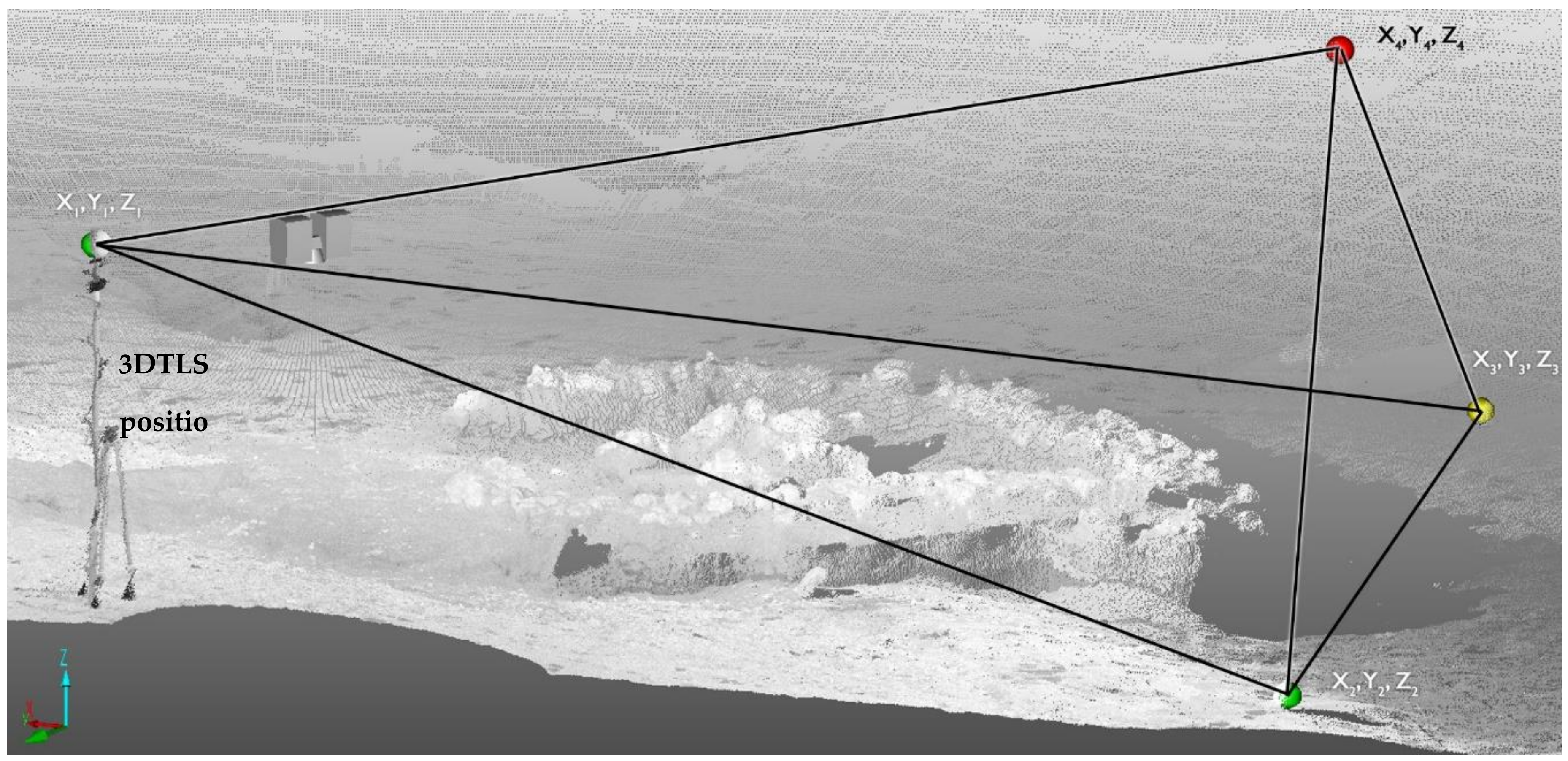
A sphere S is parameterised by its centre $c=\left(c_x,c_y,c_z\right)$ and its radius r (Figure 4). The distance of a point p from the sphere is given by:

$$d_S=\left|\left|p-c\right|\right|-r=\sqrt{{\left(p-c\right)}^T\cdot \left(p-c\right)}-r$$

(28)

Figure 5 shows the estimated quadric converted into the standard form by the method described. For the calculation of the approximate values, a quadric adjustment followed by a canonical analysis can be used. Another approximation based on the implicit sphere equation can be found in [37].

2.5. 3DTLS Networks

The approach to the type of system to be solved by means of least squares is different depending on the characteristics of the relationships established by relating the two large categories of variables, the observations and the parameters. The essential difference between the two categories is that the parameters have unknown values at the beginning of the process and are therefore functional unknowns. The vector of observations will be called L, and the vector of parameters X in the following. Observations and parameters also differ in nature in that observations are random variables, while parameters are deterministic variables ([38], p. 108) that define a given mathematical model even if their value is unknown.

2.5.1. General Adjustment Model

This least squares adjustment model appears under different names in the literature, for example, it is called general method by Chueca Pazos et al. [25], Mikhail and Ackermann [39], Cooper [40], and Wolf and Ghilani [41]; mixed adjustment model by Leick [38]; or combined by Harvey [42]. The situation is one in which observations and parameters cannot be separated, and it is necessary to work with them in implicit relationships. The method may also be necessary where there is more than one observation involved in each type of functional relationship that can be formulated.

Chueca Pazos et al. [43] particularises the methodology to the ‘topographic case’, that is, the one that represents physical terrain surfaces and keeps the axis of the coordinates permanently in the vertical direction. In the present case, local networks are dealt with, always of relatively small extension, so the topographic variation of the vertical will be disregarded, and therefore all the axes will be considered parallel.

This model of relationships can be formulated in the following way according to ([38], p. 108):

F(L_a,X_a) = 0

(29)

where L_a is the vector of adjusted observations and X_a is the vector of adjusted parameters. The stochastic model is expressed by a weight matrix that is related to the variance-covariance matrix associated with the observations by a relative scaling factor, which is called the reference variance. It is possible to put that:

$$P={\sigma }_0^2·{\Sigma }_L^{-1}$$

(30)

Linearising the equation and developing it, we can reach:

$$\widehat{X}=-{\left(A^T{M}^{-1}A\right)}^{-1}{A}^T{M}^{-1}W$$

(31)

The calculation of the cofactor matrices and the a posteriori reference variance expression can be followed in [38]. The general model described can be particularised for particular cases depending on the characteristics of the functional relationships between observations and parameters. This produces the models known as the observation or parametric equation model and the condition equation model.

Observation Equation Modelling

This variant of least squares adjustment is possible when there is an explicit relationship between observations and parameters:

$$L_a=F\left(X_a\right)$$

(32)

This variant is properly called the Gauss–Markov model whose theorem was cited above. Other authors call it the indirect observations method (Mikhail and Ackermann [39] and Chueca Pazos et al. [25]), parametric method (Harvey [42]), or observation equation model (Cooper [40] and Leick [38]).

For this model it is sufficient to particularise the general expression:

$$B=\frac{\partial \left[F\left(X_a-L_a\right)\right]}{\partial L_a}=-I$$

(33)

$$W=F\left(X_0\right)-L_b=L_0-L_b$$

(34)

It can now be written that:

$$A \cdot X+W=V$$

(35)

This method is the most frequent in programming because of its facility to generalise the process for different classes of observation equations, in such a way that an equation is posed for each observation, which makes it possible to maintain a single method of resolution for different types of problems once the different classes of observation equations have been formulated.

Conditional Equation Model

In other cases, it is possible to establish equations in which only observations are involved, thus imposing a series of conditions that must be met by the adjusted values of the observations, which is why these relationships that can be formulated are called condition equations. In this adjustment model, parameters are not involved. The equations that can be established are different for each problem, and they do not all admit this formulation. The equation is of the form:

$$F\left(L_a\right)=0$$

(36)

If we particularise the general method, we reach:

$$a=\frac{\partial \left[F\left(L_a\right)\right]}{\partial X}=0$$

(37)

Then, the final formulation will be:

$$BV+W=0$$

(38)

Resolving the problem in this way will produce only the vector of residuals to be applied to the observations.

2.5.2. Traditional Topogeodetic Observation Equations

The term ‘observation equations’ refers to the type of equations that allow an equation to be expressed as an explicit function of a set of parameters. This will be the case for the observables most frequently used in the adjustment of topographic networks. There is almost total unanimity in the denomination of these relations as ‘observation equations’; only Mikhail and Ackermann [39] call them condition equations, which can lead to confusion in some cases. This author will then call the above adjustment methods adjustments with conditions only to designate the parametric method, and adjustment with observations only to designate the condition equations fitting model. These designations do not seem to have been used by other authors.

The observation equations traditionally proposed for traditional observables vary in form depending on the reference system to be established. In the following we will work with the model of a reference system corresponding to the conformal projection plane for the observations considered in the planimetric adjustment. In any case, the reference system for the planimetric adjustment will be two-dimensional and three-dimensional.

Points of Known Coordinates

Although they are not observables that generate an equation by themselves, there are different types:

Points of known coordinates whose coordinates have a reliability higher than the laser scanner (${\sigma }_{Fixed point }<{\sigma }_{3DTLS Point}$): Generally obtained by static observations with post-processing with GNSS systems, classical techniques of series of observations, and/or micro-geodesy.

Points of known coordinates with a lower reliability than that determined by laser scanner (${\sigma }_{Fixed point }>{\sigma }_{3DTLS Point}$): Points calculated from GNSS in kinematic mode, traditional surveying methods, and so on.

Points observed by laser scanner considered as references (${\sigma }_{Fixed point }\approx {\sigma }_{3DTLS Point}$).

The values of the fixed points shall be considered for calculation as zero, and shall serve as the reference frame of the network in the linked network settings. If they are not considered as fixed, their σ will be considered in the weights matrix of observables.

Distances

Due to the technical characteristics of the 3D laser scanner, the distance equations are the most commonly used. The latter, once the observation is reduced to a conformal plane, can be written as follows:

$$S_{i,j}+v=\sqrt{{\left(x_i-x_j\right)}^2+{\left(y_i-y_j\right)}^2}$$

(39)

$$\left[{\left(\frac{x_i-x_j}{S_{i,j}}\right)}_0{\left(\frac{y_i-y_j}{S_{i,j}}\right)}_0{\left(\frac{x_j-x_i}{S_{i,j}}\right)}_0{\left(\frac{y_j-y_i}{S_{i,j}}\right)}_0\right] ·\left[\begin{array}{c}d{x}_i\\ d{y}_i\\ d{x}_j\\ d{y}_j\end{array}\right]=S_{i,j}-{\left(S_{i,j}\right)}_0$$

(40)

Some authors [44] suggest variations in the distance equation in order to take into account various errors. For example, to account for the possible introduction of systematic errors in the measurement of distances by electronic equipment, the quasi-distance is proposed:

$$S_{i,j}+v=\left(1+\mathrm{\mu }\right)\sqrt{{\left(x_i-x_j\right)}^2+{\left(y_i-y_j\right)}^2}$$

(41)

A scale factor is included in this expression to eliminate possible errors due to an inappropriate choice of refractive index, incorrect altimetric reduction, inappropriate map projection scale factor, or even systematic errors in the definition of the network datum.

Another of the equations proposed is the pseudo-distance, in which an additive term is introduced that attempts to model a systematic error combined with the instrument and prism used in the measurement of distances. The expression of this pseudo-distance is:

$$S_{i,j}+v=\sqrt{{\left(x_i-x_j\right)}^2+{\left(y_i-y_j\right)}^2}+c$$

(42)

This constant could be assimilated into what is called the ‘prism constant or reflector constant’ and is usually corrected directly by total stations from user-supplied values, depending on the reflector to be used. In both cases, the reflector constant or the scale factor represent additional parameters that need to be determined in the adjustment.

However, the distance between two or more references (see Figure 6), either spheres or targets, can also be treated as a three-dimensional distance from the position of both elements, which could be written as:

$$S_{i,j}+v=\sqrt{{\left(x_i-x_j\right)}^2+{\left(y_i-y_j\right)}^2+{\left(z_i-z_j\right)}^2}$$

(43)

$$\left[{\left(\frac{x_i-x_j}{S_{i,j}}\right)}_0{\left(\frac{y_i-y_j}{S_{i,j}}\right)}_0{\left(\frac{z_i-z_j}{S_{i,j}}\right)}_0{\left(\frac{x_j-x_i}{S_{i,j}}\right)}_0{\left(\frac{y_j-y_i}{S_{i,j}}\right)}_0{\left(\frac{z_j-z_i}{S_{i,j}}\right)}_0\right] ·\left[\begin{array}{c}d{x}_i\\ d{y}_i\\ d{z}_i\\ d{x}_j\\ d{y}_j\\ d{z}_j\end{array}\right]=S_{i,j}-{\left(S_{i,j}\right)}_0$$

(44)

An indicator of the number of points used in the adjustment of the sphere and the reliability of its position is symbolised by the colours green (>55 measured points AND position deviation < l mm), yellow (>18 points AND position deviation < l mm OR > 55 points AND position deviation > l mm), and red (none of the above conditions).

Azimuth

In 3D laser scanner networks, it is possible to enter azimuth values by placing reference spheres or targets on the points where the azimuth value is known. The azimuth equation is well known:

$${\mathsf{\theta }}_i^j+v=\arctan \left(\frac{x_j-x_i}{y_j-y_i}\right) + C$$

(45)

It is necessary to study the sign of the argument of the arc-tangent function to establish the value of the constant C, which can be worth 0^g, 200^g, or 400^g, depending on whether it is in the first, second, and third quadrant or fourth quadrant, respectively. The linearisation of the equation is:

$$F\left(x_j,y_j,x_i,x_j\right) =\arctan \left(\frac{x_j-x_i}{y_j-y_i}\right) + C=0$$

(46)

$$\left[\frac{F}{\partial x_i},\frac{F}{\partial y_i},\frac{F}{\partial x_j},\frac{F}{\partial y_j}\right] · \left[\begin{array}{c}d{x}_i\\ d{y}_i\\ d{x}_j\\ d{y}_j\end{array}\right]={\theta }_i^j-{\left(\arctan \left(\frac{x_j-x_i}{y_j-y_i}\right)+ C\right)}_0+V$$

(47)

$$\frac{F}{\partial x_i}=\frac{y_j-y_i}{S_{i,j}^2}; \frac{F}{\partial y_i}=\frac{x_j-x_i}{S_{i,j}^2}$$

(48)

$$\frac{F}{\partial x_j}=\frac{y_j-y_i}{S_{i,j}^2}; \frac{F}{\partial y_j}=\frac{x_j-x_i}{S_{i,j}^2}$$

(49)

where

$$S_{i,j}=\sqrt{{\left(x_i-x_j\right)}^2+{\left(y_i-y_j\right)}^2}$$

(50)

Horizontal Angle Readings

The horizontal angle reading is the observable obtained directly in the measurement by theodolite and total station. Its expression is related to the azimuth value of the measured direction and the angular misalignment of the station:

$$L_i^j+v={\mathsf{\theta }}_i^j-Z_i=\left(\arctan \left(\frac{x_j-x_i}{y_j-y_i}\right)+ C\right)-Z_i$$

(51)

$$F\left(x_i,y_i,x_j,x_j,Z_i\right) =\arctan \left(\frac{x_j-x_i}{y_j-y_i}\right)+ C-L_i^j-Z_i=0$$

(52)

Linearising this expression and writing the result in matrix form, taking a correction vector of the parameters as a column vector, we have:

$$\left[\frac{F}{\partial x_i},\frac{F}{\partial y_i},\frac{F}{\partial x_j},\frac{F}{\partial y_j},\frac{F}{\partial Z_i}\right]·\left[\begin{array}{c}d{x}_i\\ d{y}_i\\ d{x}_j\\ d{y}_j\\ d{Z}_i\end{array}\right]=-\left[\arctan \left(\frac{x_j-x_i}{y_j-y_i}\right)+ C\right]+Z_j+L_i^j+V$$

(53)

$$\frac{F}{\partial x_i}=\frac{y_j-y_i}{S_{i,j}^2}; \frac{F}{\partial y_i}=\frac{x_j-x_i}{S_{i,j}^2}$$

(54)

$$\frac{F}{\partial x_j}=\frac{y_j-y_i}{S_{i,j}^2}; \frac{F}{\partial y_j}=\frac{x_j-x_i}{S_{i,j}^2}; \frac{F}{\partial Z_i}=-1$$

(55)

where

$$S_{i,j}=\sqrt{{\left(x_i-x_j\right)}^2+{\left(y_i-y_j\right)}^2}$$

(56)

In the equation of the angular readings, five parameters are implied: four coordinates corresponding to the coordinates of the station points and the station’s angular misorientation. In the expression of the function, a constant C refers to the value that must be added to the result of the arc-tangent function to obtain the azimuth. The value of this constant depends on the quadrant in which the value of the angular reading is located.

As in the azimuthal case, in 3D laser scanner networks, it is possible to include horizontal angles by combining spheres and targets in the scan, thus materialising the observed angle.

Trilateration Network Adjustment

Horizontal measurements are carried out to determine the position of points accurately in planimetry. Traditionally, this has been carried out by triangulation, polygonal and trilateration. These traditional methods of measurement involve observing distance, direction, and angle. As with all measurements, there will be errors in making these measurements, and therefore they must be analysed, and if accepted, adjusted. Planimetric methods, when of significant extent, must consider systematic errors of ground curvature. One way to achieve this is to carry out the calculations using coordinates from a rigorous projection system such as UTM (Universal Transverse Mercator) or a local one that already takes curvature into account. With high-precision 3D laser scanner networks, the extension is reduced, and the effects of terrestrial curvature are negligible; therefore, the equations will be presented parametrically.

When trilaterations are adjusted using the parametric least squares method, the observation equations are expressed in a way that relates their observed quantities without inherent random errors to the most probable values for the x and y coordinates (the parameters) of the vertices. From Figure 7, the following distance equation can be written for the observation IJ.

$$d_{ij}+v_{ij}=\sqrt{{\left(x_j-x_i\right)}^2+{\left(i_j-i_i\right)}^2}$$

(57)

In the above equation, d_ij is the observed distance of a line between vertices I and J, v_dij the residual at observation d_ij, x_i and y_i the most probable coordinate values for vertex I, and _xjj and y_j the most probable coordinate values for station J. Such an equation is a non-linear function relating the variables x_i, y_i, x_j and y_j, which can be expressed as:

$$F\left(x_i,y_i,x_j,y_j\right)=d_{ij}+v_{l_{ij}}$$

(58)

where

$$F\left(x_i,y_i,x_j,y_j\right)=\sqrt{{\left(x_j-x_i\right)}^2+{\left(y_j-y_i\right)}^2}$$

(59)

A system of non-linear equations such as the above can be linearised and solved using a first-order Taylor series approximation. The linearised form of the expression is:

$$F\left(x_i,y_i,x_j,y_j\right) =F\left(x_{i0},y_{i0},x_{j0},y_{j0}\right)+{\left(\frac{\partial F}{\partial x_i}\right)}_0\cdot d{x}_i+{\left(\frac{\partial F}{\partial y_i}\right)}_0\cdot d{y}_i+{\left(\frac{\partial F}{\partial x_j}\right)}_0\cdot d{x}_j+{\left(\frac{\partial F}{\partial y_j}\right)}_0\cdot d{y}_j$$

(60)

where ${\left(\frac{\partial F}{\partial x_i}\right)}_0, {\left(\frac{\partial F}{\partial y_i}\right)}_0, {\left(\frac{\partial F}{\partial x_j}\right)}_0\mathrm{and}{\left(\frac{\partial F}{\partial y_j}\right)}_0$ are the partial derivatives of F with respect to x_i, y_i, x_j, and y_j, respectively, evaluated with the approximate coordinate values x_i0, y_i0, x_j0; while y_j0; x_i, y_i, x_j, and y_j are the unknown parameters; and dx_i, dy_i, dx_j, and dy_j are the corrections to the approximate coordinate values so that:

$$x_i=x_{i0}+d{x}_i; y_i=y_{i0}+d{y}_i$$

(61)

$$x_j=x_{j0}+d{x}_j; y_j=y_{j0}+d{y}_j$$

(62)

The calculation of the partial derivatives is straightforward and is represented as $\left(\frac{\partial F}{\partial x_i}\right).$ The distance equation can be represented as:

$$F\left(x_i,y_i,x_j,y_j\right) ={\left({\left(x_j-x_i\right)}^2+{\left(y_j-y_i\right)}^2\right)}^{\frac{1}{2}}$$

(63)

which, deriving with respect to x_i, results in:

$$\left(\frac{\partial F}{\partial x_i}\right)=\frac{1}{2}\cdot {\left({\left(x_j-x_i\right)}^2+{\left(y_j-y_i\right)}^2\right)}^{\frac{1}{2}}\cdot \left[2\cdot \left(x_j-x_i\right) \cdot \left(-1\right)\right]$$

(64)

Simplifying the equation, we arrive at:

$$\frac{\partial F}{\partial x_i}=\frac{-\left(x_j-x_i\right)}{\sqrt{{\left(x_j-x_i\right)}^2+{\left(y_j-y_i\right)}^2}}=\frac{x_i-x_j}{IJ}$$

(65)

Proceeding analogously, we arrive at:

$$\frac{\partial F}{\partial y_i}=\frac{y_i-y_j}{IJ}; \frac{\partial F}{\partial x_x}=\frac{x_j-x_i}{IJ}; \frac{\partial F}{\partial y_j}=\frac{y_j-y_i}{IJ}$$

(66)

Substituting the above equations into the linearised expression, one arrives at the general linearised distance observation expression:

$${\left(\frac{x_i-x_j}{IJ}\right)}_0\cdot d{x}_i+{\left(\frac{y_i-y_j}{IJ}\right)}_0\cdot d{y}_i+{\left(\frac{x_j-x_i}{IJ}\right)}_0\cdot d{x}_j+{\left(\frac{y_j-y_i}{IJ}\right)}_0\cdot d{y}_j$$

(67)

where ${\left( \odot \right)}_0$ is evaluated with the approximate values, $k_{l_{ij}}=l_{ij}-I{J}_0$ and

$$I{J}_0=F\left(x_{i0},y_{i0},x_{j0},y_{j0}\right)=\sqrt{{\left(x_{j0}-x_{i0}\right)}^2+{\left(y_{j0}-y_{i0}\right)}^2}$$

(68)

2.5.3. Network Datum, Constraints, and Degrees of Freedom

Within the theory of high-precision topogeodetic network design, the zero-order design problem, also known as the datum problem, is concerned with determining the optimal fixed parameter definition for each network. Generally, these parameters will be coordinates of some or all of the vertices of the network, which is the theory of free networks with or without definition of intrinsically accurate enclosures.

The observation equations are relative relationships between parameters, and therefore alone are not sufficient to obtain absolute parameter values. For example, with a topographic network, the parameters are the coordinates of the stations (and perhaps the misorientations at those stations); observations such as distances, angular readings, or angles represent relationships between those parameters that do not by themselves define a single solution for the values of the network parameters. In this way, the same planimetric network formulated only by the observation equations mentioned above, moved on the X-Y coordinate plane to another different position or rotated around one of its stations, continues to fulfil the observation equations, because these are relative or internal relationships between network parameters. However, no relationship links these parameters to the reference system to which they are referenced. This indeterminacy translates mathematically into the singular character of the matrix of coefficients of the system of normal equations, which gives rise to a system with an indeterminate solution.

The datum or zero order design problem, whatever its application, demonstrates that it is generally impossible to univocally re-state the adopted origin of coordinates, even from the first approximation. According to Chueca Pazos et al. [43], a series of error enclosures must be accepted which will contain the most probable successive origins (datums) corresponding to each adjustment made. Consequently, from any one model and starting datum to the next adjusted model and datum it is necessary to accept that the reality represented by the first model has been modified by the successive and joint application of:

• A correction to the coordinates of all vertices represented by the solution vector of the adjustment;
• A geometric transformation to the previously formed and adjusted network that keeps it the same as itself and refers it to new axes (adjusted datum).

To eliminate this singularity, it is necessary to add a series of new parameter relations which, being independent of each other and of the observation equations, make it possible to construct a single solution system, which will be the minimum quadratic solution. This process performs the definition of the network datum.

A description of the minimum number of parameters needed to define a reference system depending on the type of network in question can be found in [45] (p. 12) or [40] (p. 207).

Table 2. Minimum number of parameters needed to define the datum in different types of networks (adapted from [45,40]).

Network Type	Parameters Defining the DATUM	No. Parameters Required
Altimetric network	1 translation Tz	1
Triangulated planimetric network	2 translations Tx, Ty, 1 rotation κ 1 scale factor S	4
Trilateral planimetric network	2 translations Tx, Ty 1 rotation κ	3
3D network (with distances)	3 translations Tx, Ty, Tz 3 rotations ω, φ, κ	6
3D network (without distances)	3 translations Tx, Ty, Tz 3 rotations ω, φ, κ 1 scale factor S	7

lists these parameters for different types of networks:

The 3D Laser Scanner case is a three-dimensional network setting, as shown later. In reality, the constraints are not (or may not be) special equations distinct from the observation equations. The observation equations serve to pose constraints. What determines the difference between an observation equation and a constraint is ‘the intensity’ with which compliance with this equation is required. For example, an azimuth between two points on a planimetric network may constitute an observation or a constraint. In the latter case, the coordinates of the two points related by that azimuthal value will have to strictly comply with the relationship represented by the azimuth equation, so there will be no residual for that azimuth considered as a constraint, whereas if it intervenes in the adjustment as an observation equation, the relationship will be fulfilled, but not exactly, and the azimuth value calculated from the adjusted coordinates will differ slightly from the observed one (i.e., there will be a non-zero residual for that observation). In practice, even this difference referred to in the previous paragraph does not make a difference in some resolution methods. Some types of observations have inherent information about the geodetic datum that eliminates the need to fix any of the above parameters, for example, in [45,46] and [40] some tables can be found whose information is reproduced in

Table 3. Relationship between type of observation and datum parameters inherent to the observation (adapted from [40,45,46)].

	Datum Parameters
Observations	Tx	Ty	Tz	$\mathit{\omega }$	$\mathit{\varphi }$	$\mathit{\kappa }$	S
Angles and Angular Readings	-	-	-	-	-	-	-
Distances	-	-	-	-	-	✓	✓
Azimuths	-	-	-	-	-	-	-
Zenith Angles	-	-	-	✓	✓	-	-
Elevations	-	-	-	-	✓	✓	✓
GNSS Positions	✓	✓	✓	✓	✓	✓	✓
GNSS Baselines	-	-	-	✓	✓	✓	✓

:

When the number of independent constraints added to the system of observation equations is equal to the number needed to define the datum, the adjustment is said to be a minimum constraint adjustment; if the number of constraints is greater, the adjustment is called over-constrained. The latter type of adjustment must be applied with care since any errors in the constraints that will define the datum will be transmitted to the new adjusted network. Some of the most common constraints that may be imposed in a topographic adjustment are described below.

Points of Known Coordinates

This is one of the most common constraints and exists in virtually every adjustment, whether by 3D laser scanner or by classical surveying methods. It is either a network independent of another with greater precision or not, and it considers one of the points as a control point whose coordinates are known. The equations to be added are simply:

$$x_i=C_x ; y_i=C_{y }; z_i=C_z$$

(69)

$$d{x}_i=0; d{y}_i=0; d{z}_i=0$$

(70)

The above are the equations for a fixed point in the case of a three-dimensional network where the values C_x, C_y, and C_z are the values of the coordinates to be fixed. Since in practice, the traditional observation equations are non-linear, they have to be linearised, and their solution is proposed iteratively. The second trio of equations represents the idealised equations which impose that the corrections of the coordinates of the point to be fixed are zero in each iteration, and therefore the initial values of the parameters to be fixed undergo no change. It is possible to fix only a single coordinate, as in the altimetric adjustment where the height (or altitude) of a point is fixed.

Fixed Azimuth

The azimuth constraint of a network is reduced to the constraint of the azimuth observation equation already stated above. Basically, the azimuth equation sets a numerical relationship between the coordinates of the points involved that must be fulfilled. Therefore, it will be an adjustment with additional parameter functions.

This restriction makes it possible to ‘orient’ the network with respect to the chosen reference system, thus fixing the degree of freedom which represents the rotation around the Z axis of the whole network.

Horizontal Angular Reading to a Fixed External Point

Another way of orienting the network is to impose as a constraint the horizontal angular reading to a point outside the grid, which is fixed since its coordinates do not intervene in the adjustment. For this constraint to be effective, it must be imposed from a point on the grid that is also fixed. Thus, the parameter fixed is the misorientation of that point. The equation that formulates the constraint is identical to the one for the direction observation equation shown above.

Network Internal Constraint

The so-called internal constraint of a network in [23] (p. 211), [38] (p. 130), [46], (p. 106) (or treated under other names in the following references: [44] null space representations, [45] minimum trace datum, [25] free topographic networks) is a minimal set of constraints describing functional relationships between null space and the first order increments of the point coordinates of a network. They produce a least squares estimate with useful properties.

The constraints are imposed on a fictitious reference such as the centroid of the stations in the network calculated from the initial coordinates. In a 3D laser scanner trilaterated network, which is the case considered in this text, the conditions imposed are:

• The coordinates of the network centroid must remain unchanged after the adjustment. Therefore, if the centroid coordinates are:

  $$x_G=\frac{{{\displaystyle \sum }}_{i=1}^n{x}_i}{n}$$

  (71)

  $$y_G=\frac{{{\displaystyle \sum }}_{i=1}^n{y}_i}{n}$$

  (72)

  the restrictions to be fulfilled would be that the corrections to the centroid coordinates are zero, that is, that the centroid remains unchanged due to the adjustment:

  $$d{x}_G=0 d{y}_G=0$$

  (73)

  which implies that:

  $${\displaystyle \sum }_{i=1}^{n}d{x}_i=0 {\displaystyle \sum }_{i=1}^{n}d{y}_i=0$$

  (74)
• The mean azimuth from the centroid to each network point must remain unchanged. As it can be written for the azimuth between the centroid and any point on the network that:

  $$\tan {\mathsf{\theta }}_G^i=\frac{x_i-x_G}{y_i-y_G}$$

  (75)

  differentiating

  $$d{\mathsf{\theta }}_G^i=\frac{\left(y_i-y_G\right) · \left(d{x}_i-d{x}_G\right)-\left(x_i-x_G\right) · \left(d{y}_i-d{y}_G\right)}{{\left(x_i-x_G\right)}^2+{\left(y_i-y_G\right)}^2}$$

  (76)

Imposing that $\sum d{\mathsf{\theta }}_G^i=0$ it follows from the above expression that:

$${\displaystyle \sum }_{i=1}^n\left[\left(y_i-y_G\right) · \left(d{x}_i-d{x}_G\right)-\left(x_i-x_G\right) · \left(d{y}_i-d{y}_G\right)\right]=0$$

(77)

which in a more simplified form can be put as:

$${\displaystyle \sum }_{i=1}^n\left(y_i\cdot d{x}_i-x_i\cdot d{y}_i\right)=0$$

(78)

There is also another restriction which constrains the average distance from the centroid to each point in the network; writing the distance from the centroid to a point i as $S_G^i=\sqrt{\left(x_i-x_G^2\right)+{\left(y_i-y_G\right)}^2}$.

In the present case, a trilaterate grid, it would not be necessary to impose the equation corresponding to the distance, and the three restrictions above would be enough; that is, in all possible cases of trilateration, the scale is fixed.

Therefore, if the vector of corrections to the coordinates of the references of the fit is of the form:

$$x={\left[d{x}_1 d{y}_1 d{z}_1 d{x}_2 d{y}_2 d{z}_2\dots d{x}_n d{y}_n d{z}_n\right]}^T$$

(79)

The set of possible internal constraints can be put as the following matrix B, which will multiply the vector x as a function of each case.

• 3D trilateration: No fixed point and no orientation. There is a translation in X, Y, Z = (da, db, dc) and a rotation of axes (dω, dθ). Here, there are five degrees of freedom, and the constraint matrix will be as follows:

$$B=\left(\begin{array}{cccccccccc}1& 0& 0& 1& 0& 0& \dots & 1& 0& 0\\ 0& 1& 0& 0& 1& 0& \dots & 0& 1& 0\\ 0& 0& 1& 0& 0& 1& \dots & 0& 0& 1\\ y_1& -x_1& 0& y_2& -x_2& 0& \dots & y_n& -x_n& 0\\ 0& z_1& -y_1& 0& z_2& -y_2& \dots & 0& z_n& -y_n\end{array}\right)$$

(80)

2.

3D trilateration with known azimuth; no fixed point but with orientation. There is a translation in X, Y, Z = (da, db, dc) and an axis rotation (dθ). Here, there are four degrees of freedom, and the constraint matrix will be as follows:

$$B=\left(\begin{array}{cccccccccc}1& 0& 0& 1& 0& 0& \dots & 1& 0& 0\\ 0& 1& 0& 0& 1& 0& \dots & 0& 1& 0\\ 0& 0& 1& 0& 0& 1& \dots & 0& 0& 1\\ 0& z_1& -y_1& 0& z_2& -y_2& \dots & 0& z_n& -y_n\end{array}\right)$$

(81)

3.

3D trilateration with a fixed elevation. No fixed planimetric point, with a fixed height (or altitude) point and no orientation. There is a translation in X, Y = (da, db) and a rotation of axes (dω, dθ). Here, there are four degrees of freedom, and the constraint matrix will be as follows;

$$B=\left(\begin{array}{cccccccccc}1& 0& 0& 1& 0& 0& \dots & 1& 0& 0\\ 0& 1& 0& 0& 1& 0& \dots & 0& 1& 0\\ y_1& -x_1& 0& y_2& -x_2& 0& \dots & y_n& -x_n& 0\\ 0& z_1& -y_1& 0& z_2& -y_2& \dots & 0& z_n& -y_n\end{array}\right)$$

(82)

4.

2D trilateration, altimetry with a known fixed elevation and a fixed azimuth. No fixed planimetric point, with a fixed elevation point and orientation. There is a translation in X, Y = (da, db) and an axis rotation (dθ). Here, there are three degrees of freedom, and the constraint matrix will look like this:

$$B=\left(\begin{array}{cccccccccc}1& 0& 0& 1& 0& 0& \dots & 1& 0& 0\\ 0& 1& 0& 0& 1& 0& \dots & 0& 1& 0\\ 0& z_1& -y_1& 0& z_2& -y_2& \dots & 0& z_n& -y_n\end{array}\right)$$

(83)

5.

3D trilateration with fixed point: with a fixed point and no orientation. There is one axis rotation (dω, dθ). Here there are two degrees of freedom and the constraint matrix is:

$$B=\left(\begin{array}{cccccccccc}{y}_1& -x_1& 0& y_2& -x_2& 0& \dots & y_n& -x_n& 0\\ 0& z_1& -y_1& 0& z_2& -y_2& \dots & 0& z_n& -y_n\end{array}\right)$$

(84)

6.

3D trilateration with fixed point and known azimuth. With a fixed point and orientation. There is an axis rotation (dθ). Here, there is one degree of freedom, and the constraint matrix is:

$$B=\left(\begin{array}{cccccccccc}0& z_1& -y_1& 0& z_2& -y_2& \dots & 0& z_n& -y_n\end{array}\right)$$

(85)

This matrix B will be the matrix used to constrain the system during the adjustment, and it can be easily checked by performing the product of the matrices that B · X = 0. Therefore, this set of constraints can be used as any other set of constraints for the adjustment, following the method of adjustment with parameter functions [38], (p. 134).

There are also at least two other specific methods of imposing the internal constraint on a network. The first of these involves calculating the Moore–Penrose pseudoinverse matrix corresponding to the coefficient matrix of normal equations, ([40], p. 214; [47], p. 409; [25], Chap. 17). This method requires more computational effort, as it is necessary to calculate the singular values of the matrix to obtain the pseudoinverse, and on the other hand, it is a purely algebraic method that dispenses with the physical meaning that in geodesy or topography is associated with the internal constraint of a network (i.e., the free network adjustment). A third solution consists in using ‘S-transforms’. These transformations allow the calculation of the variance-covariance matrix of a minimum constraint adjustment from the same matrix corresponding to a different minimum constraint adjustment. ([40], p. 311; [46], p. 118).

2.5.4. Resolution Methods

Imposition of Constraints by Elimination of Parameters

This method is the classical method for imposing the datum of a geodetic network and consists of eliminating the columns of the design matrix A that refer to the parameters to be kept fixed. Its implementation is simple when the datum is defined only with positional constraints, and is less suitable if it is needed to impose other types of constraints, such as angular constraints.

The solution approach can be carried out as follows by partitioning the linear (or linearised) system of observation equations into the matrix A, assuming that the parameters to be fixed are denoted as x₂. Thus, we have:

$$\left[\begin{array}{cc}{A}_1& A_2\end{array}\right]·\left[\begin{array}{c}{x}_1\\ x_2\end{array}\right]=\mathrm{l}+\mathrm{v}$$

(86)

$$A_1 · x_1+A_2 · x_2=\mathrm{l}+\mathrm{v}$$

(87)

The range of the matrix A₁ will be equal to the number of parameters minus the rank defect of the complete matrix A, which has no rank defect. In non-linear models solved iteratively, imposing fixed parameters is done by adding equations of the type d_x = 0, so the value of the vector x₂ will be a null vector, and thus the solution of the system to be solved reduces to:

$$A_1 · x_1=l+\mathrm{v}$$

(88)

The solution being the classical one for the parametric method where A₁ is a full rank matrix and therefore invertible.

$$x_1={\left(A_1^t\cdot P\cdot A_1\right)}^{-1}\left(A_1^t\cdot P\cdot I\right)$$

(89)

$$Q_{x_1}={\left(A_1^t\cdot P\cdot A_1\right)}^{-1}$$

(90)

In other cases, as occurs in the resolution of an altimetric adjustment based on observations composed of differences in level between stations, the model will be linear, this being necessary to fix the value of the elevation of some of the stations, or several of them, which in general will not be null. The solution will then be:

$$\begin{array}{ll}{x}_1={\left(A_1^t\cdot P\cdot A_1\right)}^{-1}& \left(A_1^t\cdot P\right)\left(l-A1\cdot L\cdot x_2\right)\\ & ={\left(l-A_1^T\cdot P\cdot A_1\right)}^{-1}\cdot A_1\cdot P\cdot \left(l-A_2{x}_2\right)\end{array}$$

(91)

$$Q_{x_1}={\left(A_1^t\cdot P\cdot A_1\right)}^{-1}$$

(92)

The cofactor matrix of the parameters is independent of x₂. This resolution is the one implemented in resolving the altimetric adjustment. The columns of the complete design matrix A corresponding to the parameters to be removed are shifted to the second member in the original system multiplied by the value to be imposed on this parameter. The fixed parameters are sometimes referred to as the zero-variance basis of the model [45], and all elements of the covariance matrix must be considered as relative variances with respect to the chosen basis.

Adjustment with Parameter Functions

In the standard resolution of the adjustments, it is assumed that the coefficient matrix of the system of normal equations is of full rank and therefore has an inverse that can be calculated by the classical method. The elimination method of the previous section also finally produces a coefficient matrix for the normal system which is invertible; however, this method presents greater programming difficulties when intended to implement restrictions such as those of an azimuth or a fixed horizontal reading.

It is then possible to use as an alternative the approach set out below in which the resolution of the adjustment of a system formed by two groups of equations, one corresponding to the observations and the other corresponding to the restrictions:

$$A \cdot x=l+v$$

(93)

$$R^t\cdot x=c$$

(94)

where R is the matrix of coefficients of the set of restrictions, and c is the vector of constants. The function to minimise will be:

$$\mathsf{\varphi }=v^t\cdot P\cdot v+2\cdot k_1^t\left(l+v-A\cdot x\right)+2\cdot k_2^t\left(R^t\cdot x-c\right)$$

(95)

Deriving and imposing the minimum condition, we have:

$$\frac{\partial \mathsf{\varphi }}{\partial v}=2\cdot v^t\cdot P+2\cdot k_1^t=0\to P\cdot v+K_1=0$$

(96)

$$\frac{\partial \mathsf{\varphi }}{\partial x}=-2\cdot k_1^t\cdot A+2\cdot k_2^t\cdot RT=0\to -A^t\cdot k_1+R\cdot K_2=0$$

(97)

The original system and the above conditions can be put matrixially:

$$\left[\begin{array}{cccc}P& I& 0& 0\\ 0& -A^T& R& 0\\ I& 0& 0& -A\\ I& 0& 0& -A\\ 0& 0& 0& R^T\end{array}\right]· \left[\begin{array}{c}v\\ k_1\\ k_2\\ x\end{array}\right]=\left[\begin{array}{c}0\\ 0\\ -l\\ c\end{array}\right]$$

(98)

If we consider the following development:

$$\left[\begin{array}{cc}{P}_{11}& P_{12}\\ P_{21}& P_{22}\end{array}\right]·\left[\begin{array}{c}{y}_1\\ y_2\end{array}\right]=\left[\begin{array}{c}{u}_1\\ u_2\end{array}\right]$$

(99)

$$y_1=P_{11}^{-1}\left(u_1-P_{12}\cdot y_2\right)$$

(100)

$$\left[P_{22}-P_{21}\cdot P_{11}^{-1}\cdot P_{12}\right]=\left(u_2-P_{21}\cdot P_{11}^{-1}\cdot u_1\right)$$

(101)

and we apply successively this second expression to the previous system, we obtain:

$${\displaystyle [}\left[\begin{array}{ccc}-A^T& R& 0\\ 0& 0& -A\\ 0& 0& R^T\end{array}\right]-\left[\begin{array}{c}0\\ l\\ 0\end{array}\right]·P^{-1}·\left[\begin{array}{ccc}l& 0& 0\end{array}\right]{\displaystyle ]}·\left[\begin{array}{c}{k}_1\\ k_2\\ x\end{array}\right]=\left[\begin{array}{c}0\\ -l\\ c\end{array}\right]$$

(102)

If we repeat the process, we obtain:

$$\left[\begin{array}{cc}R& 0\\ 0& R^T\end{array}\right]-\left[\begin{array}{c}-A^T\\ 0\end{array}\right]·P·\left[\begin{array}{cc}0& -A^T\end{array}\right]=\left[\begin{array}{c}0\\ c\end{array}\right]-\left[\begin{array}{c}-A^T\\ 0\end{array}\right]·P·\left[-l\right]$$

(103)

We then arrive at the approach of the normal equations matrix as follows:

$$\left[\begin{array}{cc}{A}^T·P·A& R\\ R^T& 0\end{array}\right]·\left[\begin{array}{c}x\\ -k_2\end{array}\right]=\left[\begin{array}{c}{A}^T·P·l\\ c\end{array}\right]$$

(104)

The solution to this system can be carried out directly, by inverting the new coefficient matrix, since it is now a full rank matrix, provided that the restrictions imposed are independent. Alternatively, the expression known as the addition method of normal equations can be used:

$$x={\left(A^t\cdot P\cdot A+R\cdot R^t\right)}^{-1}\left(A^t\cdot P\cdot l+R\cdot c\right)$$

(105)

This expression can be achieved by using the method of partitioning matrices on the above system. The calculation of the cofactor matrix of the parameters must also be carried out in a special way, because the submatrix $A^t\cdot P\cdot A$ is not of full rank and therefore, as mentioned above, not invertible. However, it can be written that:

$$\left[\begin{array}{c}x\\ -k_2\end{array}\right]=\left[\begin{array}{cc}{A}^T·P·A& R\\ R^T& 0\end{array}\right]·\left[\begin{array}{c}{A}^T·P·l\\ c\end{array}\right]$$

(106)

Since the above inverse exists, this inverse matrix can be denoted by the following notation:

$${\left[\begin{array}{cc}{A}^T·P·A& R\\ R^T& 0\end{array}\right]}^{-1}=\left[\begin{array}{cc}\alpha & {\beta }^T\\ \beta & \gamma \end{array}\right]$$

(107)

The independent term, denoted in the above equation as A, is expressed as the sum of a vector of constants and a vector dependent on the weights matrix and the observations matrix, since we are looking for a linear model:

$$\left[\begin{array}{c}{A}^T·P·l\\ c\end{array}\right]=\left[\begin{array}{c}{A}^T·P·l\\ 0\end{array}\right]+\left[\begin{array}{c}0\\ c\end{array}\right]=a$$

(108)

If we now apply the law of propagation of variance-covariance to the second of the above expressions, it is possible to calculate the cofactor matrix of the term a as a function of the cofactor matrix of the vector of observations l, so that the expression obtained will be:

$$Q_a=\left[\begin{array}{c}{A}^T·P\\ 0\end{array}\right]·Q·\left[\begin{array}{cc}P·A& 0\end{array}\right]=\left[\begin{array}{cc}{A}^T·P·A& 0\\ 0& 0\end{array}\right]=\left[\begin{array}{cc}N& 0\\ 0& 0\end{array}\right]=a$$

(109)

Defining u as the vector of unknowns formed by the parameters and the Lagrange multipliers, we can calculate the cofactor matrix of this vector u as follows:

$$Q_u=\left[\begin{array}{cc}\alpha & {\beta }^T\\ \beta & \gamma \end{array}\right]·\left[\begin{array}{cc}N& 0\\ 0& 0\end{array}\right]·\left[\begin{array}{cc}\alpha & {\beta }^T\\ \beta & \gamma \end{array}\right]=\left[\begin{array}{cc}{Q}_x& Q_{xk}\\ Q_{kx}& Q_k\end{array}\right]$$

(110)

$$Q_x=\alpha \cdot N\cdot \alpha$$

(111)

However, it can also be written as follows:

$$\left[\begin{array}{cc}N& R\\ R^T& 0\end{array}\right]·\left[\begin{array}{cc}\alpha & {\beta }^T\\ \beta & \gamma \end{array}\right]=\left[\begin{array}{cc}I& 0\\ 0& I\end{array}\right]$$

(112)

$$N \cdot \alpha +R \cdot \beta =I \to N \cdot \alpha =I-R \cdot \beta$$

(113)

$$R^t\cdot \alpha =0\to \alpha \cdot R=0$$

(114)

Substituting in the expression for $Q_x$ we have:

$$Q_x=\alpha \left(I-R\cdot \beta \right)=\alpha -\alpha \cdot R\cdot \beta =\alpha$$

(115)

Therefore, the cofactor matrix of the parameters is the upper left submatrix of the inverse matrix of the coefficient matrix of the complete system. The peculiarity is this submatrix identified as N is singular.

Now, the cofactor matrix of the residuals can be calculated with the standard expression, once the cofactor matrix of the parameters is known by the previous expression.

Weighted Method

The weighted method of least squares resolution ([29], p. 192; [48], p. 138; [39], Ch. 12; [41], p. 390) is based on the consideration that there is in fact no functional difference between the observation equations and the constraints, and we can therefore consider that all the variables involved in the mathematical formulation are observations ([39], p. 334). Now, to achieve the same effect as above with the constraints, we must employ some mechanism that allows us to require the fulfilment of some of the observation equations (the old constraints) with greater intensity than the others. This mechanism will be the weight associated with each observation. If an observation is given an infinite variance, its weight will be 0, and therefore it will be able to vary freely in the adjustment; on the other hand, if an observation is given a zero variance, its weight will approach infinity and will not be allowed to change in the adjustment ([39], p. 334). It is then a matter of solving:

$$min\_x\parallel \left[\begin{array}{c}\gamma B\\ A\end{array}\right]·x-{\left[\begin{array}{c}\gamma d\\ b\end{array}\right]\parallel }_2$$

(116)

where B corresponds to the observation equations that were previously interpreted as restrictions, and $\gamma$ is the corresponding weight factor, to which very large values will be assigned. As Björk points out, the method is very attractive since, besides its apparent simplicity, it is possible to use a resolution method corresponding to unrestricted least squares, since if B and A are independent of each other, the resulting matrix in the least squares adjustment is of full rank. However, for large values of $\gamma$, the matrix is badly conditioned, and the method of normal equations will fail for large values of $\gamma$ ([29], p. 192).

2.5.5. Weighting of Observations

Introduction

When measurements are made, they normally have to meet geometric conditions; when they do not, the measurements are adjusted to force geometric closure. For a set of uncorrelated observations, a high-precision measurement, indicated by a low variance, implies a good observation, and in the adjustment should receive a relatively small correction. Conversely, a lower-precision measure, with a high variance, implies a larger error and should receive a larger portion of the correction.

The weight of an observation is a measure of its relative value, in comparison with the other measures [47]. Weights are used to control the sizes of the corrections applied to a measure in an adjustment. The more precise an observation is, the more weight it has, (i.e., the smaller the variance, the greater the weight). From the previous analysis, it can be intuitively deduced that weights are inversely proportional to variances.

In situations where measures are correlated, weights are related to the inverse of the covariance matrix, E; however, since weights are relative, variances and covariances are replaced by cofactors. A cofactor is related to the covariance by the equation:

$$q_{ij}=\frac{{\sigma }_{ij}}{{\sigma }_0^2}$$

(117)

where $q_{ij}$ is the cofactor of the ij-th measurement, ${\mathrm{\sigma }}_{ij}$ is the covariance of the y-th measurement, and ${\mathrm{\sigma }}_0$ the reference variance, which is a value that can be used for scaling [47] and can be expressed as:

$$Q=\frac{1}{{\mathrm{\sigma }}_0^2}$$

(118)

where Q is defined as the cofactor matrix, being in matrix form:

$$\Sigma =\left[\begin{array}{cccc}{\sigma }_{x1}^2& {\sigma }_{x1x2}& \cdots & {\sigma }_{x1xn}\\ {\sigma }_{x2x1}& {\sigma }_{x2}^2& \cdots & {\sigma }_{x2xn}\\ ⋮& ⋮& \ddots & ⋮\\ {\sigma }_{xnx1}& {\sigma }_{xnx2}& \cdots & {\sigma }_{xn}^2\end{array}\right]$$

(119)

$$P=Q^{-1}={\mathrm{\sigma }}_0^2\cdot {\Sigma }^{-1}$$

(120)

For uncorrelated measures, the covariances are zero, so the matrix $\sigma$ is diagonal. Thus, Q is also a diagonal matrix with elements equal to $\frac{{\mathrm{\sigma }}_{xi}^2}{{\mathrm{\sigma }}_0^2}$. The inverse of the diagonal matrix will also be a diagonal matrix, with its elements reciprocal to the elements of the original diagonal.

$$\mathrm{P}=\left[\begin{array}{cccc}\frac{{\sigma }_0^2}{{\sigma }_{x1}^2}& 0& \cdots & 0\\ 0& \frac{{\sigma }_0^2}{{\sigma }_{x2}^2}& \cdots & 0\\ 0& 0& \ddots & 0\\ 0& 0& \cdots & \frac{{\sigma }_0^2}{{\sigma }_{xn}^2}\end{array}\right]={\sigma }_0^2·\Sigma -1$$

(121)

From the above equation, it follows that any independent measure with variance equal to ${\sigma }_i^2$ has a weight of:

$$p_i=\frac{{\mathrm{\sigma }}_0^2}{{\mathrm{\sigma }}_i^2}$$

(122)

If the i-th observation has a weight of $p_i=1$, then ${\mathrm{\sigma }}_0^2={\mathrm{\sigma }}_i^2, \mathrm{or} {\mathrm{\sigma }}_0^2=1$. Thus, ${\sigma }_0^2$ is usually given the name variance of a unit weight observation [25], abbreviated in some literature to variance of unit weight [49] or simply unit variance. If ${\sigma }_0^2$ is set to 1, then:

$$p_i=\frac{1}{{\mathrm{\sigma }}_i^2}$$

(123)

With correlated observations, it is possible to have a covariance matrix, $\Sigma$, and a cofactor matrix, Q, but not a weight matrix. This is the case when the cofactor matrix is singular, and therefore there is no inverse for Q. Most situations involve uncorrelated observations. As considered in the cited texts, only the case of uncorrelated observables, which consider the unit weight variance, will be considered.

Weighted Average

When two measurements of a quantity with different qualities are taken, an adjustment of these measurements must be made to give the most probable value. The general expression for calculating the weighted mean, if we have m independent uncorrelated observations $\left(z_1,z_2,\dots ,z_m\right)$ of a quantity z where each observation has a standard deviation $\sigma$, is:

$$\overline{z_a}=\frac{{{\displaystyle \sum }}_{i=1}^m{z}_i}{m}$$

(124)

However, when these observations have a different variance, as in the case of the spheres used as references, each observation will have a weight associated with it, and the above expression can be expressed as:

$$\overline{z}=\frac{p_a\cdot \overline{z_a}+p_b\cdot \overline{z_b}+\cdots +p_m\cdot \overline{z_m}}{p_a+p_b+\cdots +p_m}=\frac{\sum p\cdot z}{\sum p}$$

(125)

This is the equation used to calculate the weighted mean for a group of uncorrelated observations having unequal weights. This value is the most probable value for a set of weighted observations [50].

Relationship between Weights and Standard Errors

Applying the law of variance propagation to the weighted weight expression, the variance $\overline{z_a}$ is:

$${\mathrm{\sigma }}_{\overline{z_a}}^2={\left(\frac{\partial \overline{z_a}}{\partial z_1}\right)}^2{\mathrm{\sigma }}^2+{\left(\frac{\partial \overline{z_a}}{\partial z_2}\right)}^2{\mathrm{\sigma }}^2+\cdots +{\left(\frac{\partial \overline{z_a}}{\partial z_{m_a}}\right)}^2{\mathrm{\sigma }}^2$$

(126)

Substituting the partial derivatives with respect to the equation leads to:

$${\mathrm{\sigma }}_{\overline{z_a}}^2={\left(\frac{1}{m_a}\right)}^2{\mathrm{\sigma }}^2+{\left(\frac{1}{m_a}\right)}^2{\mathrm{\sigma }}^2+\cdots +{\left(\frac{1}{m_a}\right)}^2{\mathrm{\sigma }}^2$$

(127)

In this way,

$${\mathrm{\sigma }}_{\overline{z_a}}^2=m_a\cdot {\left(\frac{1}{m_a}\right)}^2{\mathrm{\sigma }}^2=\frac{1}{m_a}\cdot {\mathrm{\sigma }}^2$$

(128)

In the above equation, $\sigma$ is a constant, and the weights $\overline{z_a}$ have been set to $m_a$; since the weights are relative, from the above equations we obtain that:

$$w_a=\frac{1}{\overline{z_a{}^2}}$$

(129)

In conclusion, it can be said that with uncorrelated observations, the weights of the observations are inversely proportional to their variances.

Statistics of Weighted Averages

Standard deviation: By definition, an observation is said to have a weight p when its precision is equal to the mean of the m unit-weight observations [51], whereas ${\sigma }_0$ is the standard error of an observation of weight 1, or unit weight. If $y_1,y_2,\dots ,y_n$ are observations with a standard error of ${\mathrm{\sigma }}_1,{\mathrm{\sigma }}_2,\dots ,{\mathrm{\sigma }}_n$ and weights $p_1,p_2,\dots ,p_n$, then:

$${\mathrm{\sigma }}_1=\frac{{\mathrm{\sigma }}_0}{\sqrt{p_1}},{\mathrm{\sigma }}_2=\frac{{\mathrm{\sigma }}_0}{\sqrt{p_2}},\dots {\mathrm{\sigma }}_n=\frac{{\mathrm{\sigma }}_0}{\sqrt{p_n}},$$

(130)

Given that the standard error of a group of equally weighted observations is defined as:

$$\mathrm{\sigma }=\sqrt{\frac{{{\displaystyle \sum }}_{i=1}^n{\epsilon }_i^2}{n}}$$

(131)

Now that the observations do not have equal weight, the above equation becomes:

$$\mathrm{\sigma }=\sqrt{\frac{p_1\cdot {\epsilon }_1^2+p_2\cdot {\epsilon }_2^2+\cdots +p_n\cdot {\epsilon }_n^2}{n}}=\sqrt{\frac{{{\displaystyle \sum }}_{i=1}^n{p}_i\cdot {\epsilon }_i^2}{n}}$$

(132)

which, modified to calculate the standard deviation, results in:

$$s=\sqrt{\frac{p_1\cdot v_1^2+p_2\cdot v_2^2+\cdots +p_n\cdot v_n^2}{n-1}}=\sqrt{\frac{{{\displaystyle \sum }}_{i=1}^n{p}_i\cdot v_i^2}{n-1}}$$

(133)

Standard error of weight and weighted mean: Combining the above expressions, the standard error of weight p is obtained in terms of ${\sigma }_0$, as follows:

$${\mathrm{\sigma }}_1=\frac{{\mathrm{\sigma }}_0}{\sqrt{p_1}}=\sqrt{\frac{\Sigma p{\epsilon }^2}{n}}\frac{1}{\sqrt{p_1}}=\sqrt{\frac{\Sigma \cdot p\cdot {\epsilon }^2}{n\cdot p_1}}$$

(134)

$$\begin{gathered} {\mathrm{\sigma }}_2=\frac{{\mathrm{\sigma }}_0}{\sqrt{p_2}}=\sqrt{\frac{\Sigma p{\epsilon }^2}{n}}\frac{1}{\sqrt{p_2}}=\sqrt{\frac{\Sigma \cdot p\cdot {\epsilon }^2}{n\cdot p_2}} \\ ⋮ \end{gathered}$$

(135)

$${\mathrm{\sigma }}_n=\frac{{\mathrm{\sigma }}_0}{\sqrt{p_n}}=\sqrt{\frac{\Sigma p{\epsilon }^2}{n}}\frac{1}{\sqrt{p_n}}=\sqrt{\frac{\Sigma \cdot p\cdot {\epsilon }^2}{n\cdot p_n}}$$

(136)

Similarly, the standard deviations of weight p can be expressed as:

$$s_1=\sqrt{\frac{\Sigma p{v}^2}{p_1\cdot \left(n-1\right)}},s_2=\sqrt{\frac{\Sigma p{v}^2}{p_2\cdot \left(n-1\right)}},\dots ,s_n=\sqrt{\frac{\Sigma p{v}^2}{p_n\cdot \left(n-1\right)}},$$

(137)

Finally, the standard error of the weighted mean is calculated as:

$${\mathrm{\sigma }}_{\overline{M}}=\sqrt{\frac{\Sigma \cdot p\cdot {\epsilon }^2}{n\cdot \Sigma \cdot p}}$$

(138)

and the standard error of the weighted mean is:

$${\mathrm{\sigma }}_{\overline{M}}=\sqrt{\frac{\Sigma \cdot p\cdot v^2}{\left(n-1\right)\cdot \Sigma \cdot p}}$$

(139)

2.5.6. Termination of Iteration

When programming a non-linear least squares adjustment, different criteria have to be established to determine the appropriate point at which to stop the iterative process [52,53,54]. Since it is possible to have a data set that has no solution, it is very important to determine when such a condition occurs. The three most commonly used methods for indicating the appropriate time of the iterative process are described below.

Maximum iterations method: The simplest iteration termination process involves limiting the number of iterations to a predetermined maximum. The risk with this method is that if the maximum is too low, a solution may not be found at the conclusion of the process, and if it is too high, time is wasted in unnecessary iterations.

Although this method does not ensure convergence, it can prevent the adjustment from continuing indefinitely, which could occur if the solution diverged. When a good initial approximation of the unknown parameters is available, 10 iterations should be sufficient to obtain the solution, as the least squares method converges quadratically.

Maximum correctness: This has an associated tracking of the absolute value of the corrections. When all the corrections become negligible, the iterative process stops. The term negligible is relative, as it is generally assumed that a correction is negligible when it is smaller than half of the smallest unit measured.

Although the solution may continue to converge with continued iterations, the work to obtain such corrections is not guaranteed due to the precision of the observations.

Tracking the reference variance of the fit: The best method for determining convergence involves tracking the reference variance and its changes between iterations. Since the least squares method converges quadratically, the iteration process should stop when the reference variance increases. An increase in the reference variance suggests a divergent solution, which occurs when one of the following happens:

• There is a gross error in the data, and it is impossible to find a solution, or
• The maximum size of the correction is smaller than the precision of the observations.

In the second case, the best solution for the given data will already have been reached, and when another iteration is performed, the solution will converge, only to diverge in the next iteration. This apparent bounce in the solution is because the convergence bounds are too tight for the quality of the data.

By tracking the reference variance, convergence and divergence can be detected. Convergence is assumed to occur when there is a change in the reference variance below a predefined percentage. Convergence can generally be assumed when the change in the reference variance is less than 1% between iterations. If the size of the reference variance increases, the solution diverges, and the iteration process should be stopped. It should be noted that tracking changes in the reference variance will always show the convergence or divergence of the solution, and this is therefore better than any previous method. However, the methods should be used in combination when performing a fit.

2.5.7. Main Design Problem: Measures of Accuracy and Reliability

The zero-order design problem, also known as the datum problem, has been addressed above. It tries to determine the optimal fixed parameter definition for each network. The main design problem is the one that studies its quality or the optimal definition of the uncertainty enclosures of a network, since only from the most rigorous knowledge of the uncertainty of the network can we go deeper into the optimisation of its design [43].

First of all, the aspects relating to accuracy, reliability, and economy must be described. Accuracy can be understood as the description of how the quality of the observations affects the fitting results through the network geometry. Reliability of a network, however, refers to how the network reacts to small deviations of the observations; it refers to the robustness of the network, that is, the ability to resist undetectable gross errors in the observations. In other words, it refers to the controllability of the observations, that is, the ability to detect errors and to estimate the effects of undetected errors on the solution. ([38], p. 161). To assess these aspects, it is possible to use multiple indicators, both global and local. The most common are local and relative error ellipses as indicators of accuracy, and internal redundancy numbers and external reliability parameters for reliability.

In this text, a multivariate analysis is used to obtain error enclosures, from which the classical ones are a generalisation, including vertex and relative error ellipses, which better interpret the uncertainty of the network. The new hyper-enclosures [25,43] have also been taken into account.

Absolute and Relative Error Ellipses

The standard deviations of the coordinates of a network point can be calculated from the variance-covariance matrix of the parameters. These variances give an indication of the error estimate in the x and y axis directions, so one could think of defining a ‘standard error rectangle’ [41] of dimensions $2{\sigma }_x$ and $2{\sigma }_y$ as defining the error area of the station; however, the least square solution of both the x and y coordinates are random variables following a bivariate normal distribution, which is the one describing the positional error of a station. It is of interest to know the accuracy of the coordinates of the spheres (with previous stations) in any direction, not only in the x and y directions. Demonstration of the calculation of the parameters associated with the error ellipse can be found in almost all reference texts ([25,27,35,36,37,38,55], etc.). Let us look at one of the possible justifications.

We can define a new system of axes (u,v), which we will relate to the system (x,y) with a rotation in the plane:

$$\left[\begin{array}{c}{u}_i\\ v_i\end{array}\right]=\left[\begin{array}{cc}\sin \left(t\right)& \cos \left(t\right)\\ -\cos \left(t\right)& \sin \left(t\right)\end{array}\right]·\left[\begin{array}{c}{x}_i\\ y_i\end{array}\right]$$

(140)

where t is the angle formed by the positive semi-axis of ordinates with the positive semi-axis of the new abscissa u, so t defines the azimuth of the positive semi-axis u. Writing the above expression in matrix form:

$$Z=R \cdot X$$

(141)

Applying the law of variance propagation, it can be written:

$${\Sigma }_{ZZ}={\mathrm{\sigma }}_0^2\cdot R\cdot Q_{xx}\cdot R^T$$

(142)

Since

$${\Sigma }_{XX}={\mathrm{\sigma }}_0^2\cdot Q_{xx}$$

(143)

where

$$Q_{xx}=\left[\begin{array}{cc}{q}_{xx}& q_{xy}\\ q_{yx}& q_{yy}\end{array}\right]$$

(144)

Then,$Q_{ZZ}$ will be:

$$Q_{ZZ}=R\cdot Q_{XX}\cdot R^T$$

(145)

$$Q_{ZZ}=\left[\begin{array}{cc}\left(\begin{array}{c}{\sin }^{2}t\cdot q_{xx}+\cos t\cdot \sin t\cdot q_{xy}\\ \sin t\cdot \cos t\cdot q_{xy}+{\cos }^{2}t\cdot q_{yy}\end{array}\right)& \left(\begin{array}{c}-\cos t\cdot \sin t\cdot q_{xx}+{\sin }^{2}t\cdot q_{xy}\\ -{\cos }^{2}t\cdot q_{xy}+\sin t\cdot \cos t\cdot q_{yy}\end{array}\right)\\ \left(\begin{array}{c}-\sin t\cdot \cos t\cdot q_{xx}+{\cos }^{2}t\cdot q_{xy}\\ {\sin }^{2}t\cdot q_{xy}+\cos t\cdot \sin t\cdot q_{yy}\end{array}\right)& \left(\begin{array}{c}{\cos }^{2}t\cdot q_{xx}-\sin t\cdot \cos t\cdot q_{xy}\\ -\cos t\cdot \sin t\cdot q_{xy}+{\sin }^{2}t\cdot q_{yy}\end{array}\right)\end{array}\right]$$

(146)

Taking the element $q_{uu}$ of the matrix, it can be put as:

$$q_{uu}={\sin }^{2}t\cdot q_{xx}+2\cdot \cos t\cdot \sin t\cdot q_{xy}+{\cos }^{2}t\cdot q_{yy}$$

(147)

with:

$$\sin 2t=2\cdot \sin t\cdot \cos t$$

(148)

$$\cos 2t={\cos }^{2}t-{\sin }^{2}t$$

(149)

$$q_{uu}={\sin }^{2}t\cdot q_{xx}+{\cos }^{2}t\cdot q_{yy}+2\cdot \frac{\sin 2t}{2}{q}_{xy}$$

(150)

Operating on the above expression, we have that:

$$\begin{gathered} q_{uu}=\frac{q_{xx}+q_{yy}}{2}\left[{\sin }^{2}t+\cos t\right]+\frac{q_{xx}\cdot {\sin }^{2}t}{2}+\frac{q_{yy}\cdot {\cos }^{2}t}{2}-\frac{q_{yy}\cdot {\sin }^{2}t}{2} \\ \hspace{1em}-\frac{q_{xx}\cdot {\cos }^{2}t}{2}+\sin 2t\cdot q_{xy} \end{gathered}$$

(151)

From where:

$$q_{uu}=\frac{q_{xx}+q_{yy}}{2}+\frac{q_{yy}}{2}\cdot \left[{\cos }^{2}t-{\sin }^{2}t\right]+q_{xy}\cdot \sin 2t$$

(152)

$$q_{uu}=\frac{q_{xx}+q_{yy}}{2}+\frac{q_{yy}-q_{xx}}{2}\cdot \cos 2t+q_{xy}\cdot \sin 2t$$

(153)

To find the maximum and minimum of $q_{uu}$ derived with respect to t:

$$\frac{d{q}_{uu}}{dt}=\frac{q_{yy}-q_{xx}}{2}\cdot 2\left[-\sin 2t\right]+q_{xy}\cdot 2\cdot \cos 2t=0$$

(154)

Finally, the above expression can be put as:

$$\tan 2t=\frac{2\cdot q_{xy}}{q_{yy}-q_{xx}}$$

(155)

This expression allows the calculation of the angle 2t, for which it is necessary to study the sign. In the same way, it can be written for $q_{vv}$ that:

$$q_{vv}=q_{xx}\cdot {\cos }^{2}t-2\cdot q_{xy}\cdot \cos t\cdot \sin t+q_{yy}\cdot se{n}^{2}t$$

(156)

It can therefore be summarised that once the value of t has been calculated, it is possible to calculate $q_{uu}$ and $q_{vv}$, and from them:

$${\mathrm{\sigma }}_{uu}={\mathrm{\sigma }}_0\cdot \sqrt{q_{uu}}$$

(157)

$${\mathrm{\sigma }}_{vv}={\mathrm{\sigma }}_0\cdot \sqrt{q_{vv}}$$

(158)

These values obtained correspond to the major and minor semi-axes of the standard error ellipse corresponding to a probability of 39.4%. This is not an adequate probability level, and it is necessary to calculate the values of the semi-axes for other probability levels, for which the expansion factors corresponding to the desired probability levels are calculated.

The calculation of the error ellipses is based on the variance-covariance matrix of the parameters, calculated once the adjustment has been solved by inverting the matrix of normal equations and scaling this matrix with the value of the reference variance or unit variance. There is a diversity of opinions among authors as to whether this scaling should be carried out based on the a priori or a posteriori reference variance.

Some limit themselves to expressing the two possibilities by specifying the cases of known or unknown unit reference variance ([44], p. 340; [46], p. 165), noting especially the different distribution function to be used in both cases for the calculation of the expansion factors during the calculation of the half-axes of the error ellipse for a given confidence level (if ${\sigma }_0$ is known, the ${\chi }^2$ distribution with 2 degrees of freedom of the adjustment will be used, while if it is unknown, the Fisher distribution will be used $F_{1-\alpha }\left(2,r\right)$).

$$a=c\cdot {\mathrm{\sigma }}_{uu};c=\sqrt{2\cdot F_{1-\alpha }\left(2,r\right)}$$

(159)

$$b=c\cdot {\mathrm{\sigma }}_{vv};c=\sqrt{2\cdot F_{1-\alpha }\left(2,r\right)}$$

(160)

Alternatively, if the a priori reference variance has been used, then:

$$a=c\cdot {\mathrm{\sigma }}_{uu};c=\sqrt{2\cdot {\mathrm{\chi }}_{1-\alpha }^2\left(2\right)}$$

(161)

$$b=c\cdot {\mathrm{\sigma }}_{vv};c=\sqrt{2\cdot {\mathrm{\chi }}_{1-\alpha }^2\left(2\right)}$$

(162)

Besides this rigorously statistical consideration, much less precise remarks are made on the practical side. In general, the problem is considered after obtaining the result of the so-called ‘goodness-of-adjustment test’, together with the level of reliability that the user assumes for the weight matrix that has been involved in the fit. If the test results in a rejection of the null hypothesis of equality of the reference variance a priori and a posteriori, a problem in the adjustment is declared to exist. There are then at least two basic possibilities that may have caused this rejection: the existence of errors in the observations, which would come with abnormally large residuals in the fit, or an erroneous assignment of weights on the observations. Logically, other causes can lead to the rejection of the test on the reference variance, such as the poor choice of the mathematical model or the existence of systematic errors in the observations. Of these two causes, the first is more unlikely in our case, and the second should manifest itself in distributing the residuals, either in magnitude or sign or both. In practice, however, several of these causes may converge and with different intensities, making it more difficult to establish the reason for rejection of the test.

Relative standard error ellipses can be calculated for a pair of points on a planimetric grid. The coordinate differences for a pair of points can be written as:

$$\left[\begin{array}{c}∆x\\ ∆y\end{array}\right]=\left[\begin{array}{cccc}-1& 0& 1& 0\\ 0& -1& 0& 1\end{array}\right]·\left[\begin{array}{c}{x}_1\\ y_1\\ x_1\\ y_1\end{array}\right];$$

(163)

$$∆=B \cdot y$$

(164)

If the variance-covariance matrix of all the points of the adjusted network is known, it is possible to construct the matrix I y for each pair of points, and applying the law of variance propagation, one will have:

$${\Sigma }_y=\left[\begin{array}{cccc}{\sigma }_{X_1,X_1}^2& {\sigma }_{X_1,Y_1}^2& {\sigma }_{X_1,X_2}^2& {\sigma }_{X_1,Y_2}^2\\ & {\sigma }_{Y_1,Y_1}^2& {\sigma }_{Y_1,X_2}^2& {\sigma }_{Y_1,Y_2}^2\\ & & {\sigma }_{X_2,X_2}^2& {\sigma }_{X_2,Y_2}^2\\ simmetric& & & {\sigma }_{Y_2,Y_2}^2\end{array}\right]$$

(165)

$${\Sigma }_{∆}=\left[\begin{array}{cc}{\sigma }_{∆X}^2& {\sigma }_{∆X, ∆Y}^2\\ {\sigma }_{∆Y, ∆X}^2& {\sigma }_{∆Y}^2\end{array}\right]=B·{\Sigma }_y·B^T=\left[\begin{array}{cc}{\mathrm{\sigma }}_{X_1}^2+{\mathrm{\sigma }}_{X_2}^2-2{\mathrm{\sigma }}_{X_1,X_2}& {\mathrm{\sigma }}_{X_1,Y_1}-{\mathrm{\sigma }}_{X_1,Y_2}-{\mathrm{\sigma }}_{X_2,Y_1}+{\mathrm{\sigma }}_{X_2,Y_2}\\ simmetric& {\mathrm{\sigma }}_{Y_1}^2+{\mathrm{\sigma }}_{Y_2}^2-2{\mathrm{\sigma }}_{Y_1,Y_2}\end{array}\right]$$

(166)

Now, the ${\Sigma }_{∆}$ matrix can be used as a submatrix of any reference to calculate the parameters of the relative ellipse [40,44]. Considering the possibility of a priori misallocation of the weights, at least two solutions are proposed. The first possibility is the rescaling of the a priori variance-covariance matrix with another value of the a priori reference variance ([40], p. 298; [46], p. 131) although this possibility would solve the problem in those cases where all the observations were of the same type (think, for example, of the case of the adjustment of a pure trilateration network). The other possibility consists of changing the relative weight distribution between groups of observations of a different nature from those involved in the adjustment.

If in the ‘goodness-of-adjustment test’ the null hypothesis is not rejected at the chosen confidence level, there is a diversity of opinions. Some ([41], p. 291; [40], p. 298) explicitly state that in this case, the value of the a posteriori reference variance is only an estimate of the true value of the a priori reference variance, and therefore it is the latter value that should be used to scale the cofactor matrix of the parameters, whereby in most cases ${\Sigma }_{\mathrm{X}}=Q_X$, since unity is taken as the value of the reference variance. This will be the criterion followed in the calculations of the current paper. Other authors ([38], p. 184) use the reference variance a posteriori for the computation of ${\Sigma }_X$.

If during the ‘goodness-of-adjustment test’ the null hypothesis is rejected, the value of the a posteriori reference variance would be biased by some causes mentioned above, so it would not be useful for calculating the parameters of the error ellipse, as this can produce enormous magnitude values with detrimental effects on the stability of the program. For this reason, in this case also the a priori reference variance shall be used in the calculation of the parameters of the ellipse. The user should note that obtaining ‘reasonable’ values for the semi-axes of the error ellipses cannot be taken as a sign of a good fit, unless the ‘goodness-of-adjustment test’ of the fit has been passed. The user is presented, in the results windows, with the values of the variances of the a posteriori references and the diagnosis of the ‘goodness-of-adjustment test’.

Uncertainty Hyper-Enclosures

The definition of the uncertainty hyper-enclosure is rigorous and clear, but unfortunately impractical or simply inapplicable in directly interpreting results in specific cases, and it is necessary to establish simplification hypotheses, or at least worth considering.

Chueca Pazos et al. [43] states that so far, a simplification hypothesis that relates each vertex, of the network or correlative, to the section of the error hypercylinder by planes generated by pairs of reference axes has been developed. However, a satisfactory application hypothesis has not yet been found, so the known one is completed to obtain much information.

The planes defined so far are sections of the general error enclosure containing two straight lines (the axes defined above) contained in the survey plane. Any other section has no representation on the survey plane and any figure represented has no physical significance in this subspace R².

In other words, from the general hyperquadric of the network, the specific error enclosures of the survey points are extracted. It is yet to be proven to be the best, but [43] formulates two more criteria to advance the knowledge of the a priori and posteriori error figures of the network within the principal design problem:

Error figures in the planimetric assumption are as follows:

• Projections of the a priori or a posteriori hyperquadric on any plane defined by two coordinate axes. This gives rise to another meaning of vertex and correlation ellipses, geometrically representative of the location of the exact vertex if the reference vertex is that of the grid or, otherwise, that of a point determined by the correlation between two vertex coordinates.
• Projection of the pairs of semi-axes on the coordinate planes formed by the generic axes. This gives rise to another meaning of ellipses of vertices and correlation of the survey, which is just as representative as the previous case. They consider issues related to the range of the design matrices.

Error figures in the three-dimensional assumption are as follows:

• Projections of the hyperquadric a priori or a posteriori onto any three-dimensional space defined by three coordinate axes. This gives rise to another meaning of vertex ellipses and correlation ellipses, geometrically representative of the location of the exact vertex if the reference vertex is of the network or, otherwise, of that of a point determined by the correlation between two vertex coordinates.
• Projection of triads of semi-axes onto any three-dimensional space defined by three coordinate axes. This gives rise to another meaning of vertex ellipses and survey correlation, which is equally representative as the previous case. The solutions depend on the range of the design matrices.

In our practical case, the error figures have been considered in the planimetric assumption, cutting the uncertainty enclosure on the co-ordinate planes, to obtain error figures representable in the subspace R² of the survey and easier to interpret.

To do so, it will relate the a priori hyperellipsoid to the a posteriori one using $\widehat{{\mathrm{\sigma }}_0^2}$, obtaining the following expression:

$$HE{S}_{\alpha }\equiv \Sigma s_{ii}\cdot x_i^2+\Sigma \cdot 2\cdot s_{ij}\cdot x_i\cdot x_j-f_{\alpha }^2=0$$

(167)

with i, j $ϵ$ 1, 2, 3, …, n and $s_{ij}=s_i$, which highlights the symmetry condition regarding the origin of coordinates, the centre of the hyperquadric.

At any point it would be possible to raise a coordinate plane $x_i$, $x_j$, (n-2) with straight lines orthogonal to it, each of them parallel to the rest of the co-ordinate axes $x_1$, $x_2$,…, $x_n$ other than those of the chosen plane.

Given an arbitrary line $r_m$ parallel to the $x_m$ axis passing through a point of arbitrary coordinates ($x_i$, $x_j$) of the survey and situated in the repeated coordinate plane, its expression could be simplified to:

$$x_k=0$$

(168)

$$\forall k \ne i, j, m$$

(169)

and cutting the hyperellipsoid by $r_m$ according to the above expression results in:

$$s_{ii}\cdot x_i^2+s_{jj}\cdot x_j^2+s_{mm}\cdot x_m^2+2\cdot s_{ij}\cdot x_i\cdot x_j+2\cdot s_{im}\cdot x_i\cdot x_m+2\cdot s_{jm}\cdot x_j\cdot x_m-f_{\alpha }^2=0$$

(170)

This expression shows that for each pair of values $x_i$, $x_j$ will cut the hypercylinder or hyperellipsoid at two points whose coordinates on the $x_m$-axis will be the solutions of the second degree equation at $x_m$.

The tangency condition $r_m$ to the hyperellipsoid is obtained by cancelling the discriminant, giving rise to:

$$4\cdot {\left(s_{im}\cdot x_i+s_{jm}\cdot x_j\right)}^2-4\cdot \left(s_{ii}\cdot x_i^2+s_{jj}\cdot x_j^2+2\cdot s_{ij}\cdot x_i\cdot x_j-f_{\alpha }^2\right) =0$$

(171)

and operating:

$$\left(s_{im}^2-s_{mm}\cdot s_{ii}\right)\cdot x_i^2+\left(s_{jm}^2-s_{mm}\cdot s_{jj}\right)\cdot x_j^2+2\cdot \left(s_{im}\cdot s_{jm}-s_{ij}\cdot s_{mm}\right)\cdot x_i\cdot x_j+s_{mm}\cdot f_{\alpha }^2=0$$

(172)

which represents the (n − 2) straight section ellipses on the $x_i$, $x_j$ plane of the survey with or without a centre at the vertex, depending on whether they are of this denomination or correlative. Its geometric configuration, as the axes of the component ellipses have different orientations, will be a rosette with central symmetry. The information obtained shall consist of N vertex rosettes and N (N-l) relative rosettes.

Redundancy Numbers

The following expression has been obtained for the cofactor matrix of the residues:

$$Q_V=P^{-1}-A\cdot N^{-1}\cdot A^T$$

(173)

Calculating its trace will give [38]:

$$\begin{array}{ll}\hfill Tr(Q\_\left\{V\right\} \cdot P& =Tr(I-A \cdot N^\left\{-1\right\} \cdot A^\left\{T\right\}\\ & =Tr\left(I\right)-Tr\left(A \cdot N^\left\{-1\right\} \cdot A^\left\{T\right\}\right)=n-u\end{array}$$

(174)

where n is the number of observation equations and u is the number of parameters. The difference n − u is the number of degrees of freedom of the fit. Therefore, the sum of the elements of the diagonal of the $Q_V\cdot P$ matrix is equal to the number of degrees of freedom of the fit. Each element of the above diagonal is called the redundancy number and is associated with each observation and represents the contribution of the observation to the number of degrees of freedom of the system. If the weights matrix is diagonal, it can be written that $r_i=q_{V{V}_i}-p_i$, so that the redundancy number depends on the weight and the element of the diagonal corresponding to that observation. From the above expression for $Q_V$ it can be deduced if the weight matrix is diagonal that:

$$0\le q_i\le \frac{1}{p_i}$$

(175)

and multiplying by $p_i$ gives $0<r_i<1$. A redundancy number equal to one indicates a certain observation (e.g., a distance between two fixed points in the case of trilateration). A redundancy number equal to zero indicates an observation without any check at all (e.g., in a topographic radiation) [42]. Leick ([38], p. 163) reasons from the expression: $Q_{La}=Q_{Lb}-Q_V$ by saying that the imprecision associated with the observations is shared between the residuals and the fitted observations. Logically, it is preferable that most of that indeterminacy is associated with the residuals so the fitted observations achieve a higher precision in that case $Q_V$ will be close to $Q_{Lb}$, so in the product $Q_V\cdot P$, the elements of the diagonal are close to 1. If $r_i$ is close to 0, then the diagonal element of the matrix Qv is expected to be small, and therefore a small amount of the random noise accompanying the observations has been transferred to the residuals.

The average redundancy number of the network is defined as:

$$r_{av}=\frac{n-u}{n}=\frac{r}{n}$$

(176)

Comparing the redundancy numbers of the observations belonging to different areas of the network with the average redundancy number allows us to discover weaker areas of the network. On the other hand, Harvey [42] cites some examples of redundancy number values for different kinds of networks (

Table 4. Examples of values of redundancy numbers for different classes of networks according to [42].

Type of Network	Typical Redundancy Number
Radiations	0
Polygonal	0.1–0.2
Level	0.2–0.5
Trilateral Nets	0.3–0.6
Networks with Distances and Angular Readings	0.5–0.8

):

Redundancy numbers depend on the weight matrix and the network design matrix A and are therefore indicators that can be calculated during the design phase based on the expected quality of the planned observations and the geometrical configuration of the network. Associated with the concept of redundancy number is the concept of ‘minimum marginal detectable error’.

External Reliability

It is not enough to ensure only good internal reliability, as this does not automatically guarantee reliable parameters. External reliability deals with the influence of undetectable errors of the observations on the parameters. This is especially important, for example, in deformation analysis.

Suppose that there is an error of magnitude ${\nabla }_i$, in the i-th observation. The least square solution in a general case where the singularity of the coefficient matrix of the system of normal equations has been eliminated can be put as:

$$\widehat{x}=-N^{-1}\cdot A^T\cdot P\cdot \left(L-e_i\cdot {\nabla }_i\right)]$$

(177)

$$e_i={\left[\begin{array}{ccc}0& 0& \begin{array}{ccc}\cdots & 0& \begin{array}{ccc}1& 0& \begin{array}{cc}\cdots & 0\end{array}\end{array}\end{array}\end{array}\right]}^T$$

(178)

The error effect on a single observation affects the whole vector of parameters, so that we can write the error that is transmitted to the parameters with the following expression:

$$\nabla X=N^{-1}\cdot A^T\cdot P\cdot e_i\cdot {\nabla }_i$$

(179)

In this way, it is possible to calculate the errors that will induce the undetected errors of the observations on the parameters. Since there are n observations, it is possible to calculate n different vectors expressing the different influences of gross errors on the fit [38].

According to Leick ([38], p. 169), the following parameter can be used as a measure of the external reliability of the network:

$${\lambda }_{0i}^2=\frac{\nabla X{}_{0i}{}^T\cdot N\cdot \nabla X_{0i}}{{\sigma }_0^2}$$

(180)

where:

$$\nabla X_{0i}=N^{-1}\cdot A^T\cdot P\cdot e_i\cdot {\nabla }_{0i}$$

(181)

where ${\nabla }_{0i}$ is the limit of the detectable marginal error. In that situation, it can be put that:

$${\mathrm{\lambda }}_{0i}^2=\frac{{\nabla }_{0i}\cdot e_i^T\cdot P\cdot A\cdot N^{-1}\cdot A^T\cdot P\cdot e_i\cdot {\nabla }_{0i}}{{\mathrm{\sigma }}_0^2}=\frac{{\nabla }_{0i}^2\cdot e_i^T\cdot P\cdot \left(I-Q_V\cdot P\right)\cdot e_i}{{\sigma }_0^2}=\frac{{\nabla }_{0i}^2\cdot p_i\cdot \left(1-r_i\right)}{{\sigma }_0^2}$$

(182)

Therefore, if the values of ${\mathrm{\lambda }}_{0i}$ are approximately equal, the network is homogeneous with respect to the reliability of its parameters. On the other hand, if the redundancy numbers are low, the external reliability factor increases, and the distortion produced on the parameters by an error can be high.

2.5.8. Post-Adjustment Statistical Analysis

Post-adjustment statistical analysis concentrates on the detection of coarse errors of small magnitude. Errors of large magnitude are easily detectable since they produce large residuals in the observations of a specific area of the network, and even in cases of linearised problem solving, they can cause the non-convergence of the process. This analysis is based on statistical tests on the residuals of the observations.

Goodness-of-Adjustment Test

This is also called the ‘global test’ or chi-square test and is used to determine whether the a posteriori reference variance ${\mathrm{\sigma }}_0^2$ is compatible with the reference variance a priori. The statistic used in the test is [43]:

$$y=\frac{r\cdot \widehat{{\mathrm{\sigma }}_0^2}}{{\mathrm{\sigma }}_0^2}$$

(183)

where r is the number of degrees of freedom of the fit. Under the null hypothesis, it can be shown that the statistic follows a distribution ${\mathrm{\chi }}^2\left(r\right)$ with r degrees of freedom, so since the mathematical expectation of ${\mathrm{\chi }}^2\left(r\right)$ is r, we can say that:

$$E\{y|H_0\}=r\Rightarrow E\{\frac{\widehat{{\mathrm{\sigma }}_0^2}}{{\mathrm{\sigma }}_0^2}\left|H_0\}=1\Rightarrow E\{\widehat{{\mathrm{\sigma }}_0^2}\right|H_0\}={\mathrm{\sigma }}_0^2$$

(184)

Therefore, the null hypothesis of the test states the statistical equality between the a priori and posteriori reference variances. If we set a significance level $\alpha$ for the two-tailed hypothesis test, the null hypothesis will be accepted if the statistic satisfies that:

$${\mathrm{\chi }}_{\alpha /2}^2\left(r\right) \le y \le {\mathrm{\chi }}_{1-\alpha /2}^2\left(r\right)$$

(185)

Either an incorrect distribution of the weights of the observations or the existence of gross errors in the observations can be considered as causes of the failure of the above test. In order to be able to discern which of these two possible causes leads to the failure of the test, it is convenient to analyse the vector of the residuals. The existence of a gross error in the observations will result in residuals of high magnitudes and with a mean different from zero. If, on the other hand, the residuals appear to be of reasonable magnitude, the first of the causes should be considered.

The statistic y depends exclusively on the vector residuals and the variance-covariance matrix of the observations, as can be seen when recalling the expression of the calculation of the reference variance a posteriori:

$$\left.\begin{array}{c}y=\frac{r\cdot \widehat{{\mathrm{\sigma }}_0^2}}{{\mathrm{\sigma }}_0^2}\\ \widehat{{\sigma }_0^2}=\frac{v^T\cdot P\cdot v}{r}=\frac{v^T\cdot {\sigma }_0^2\cdot {\Sigma }^{-}1\cdot v}{r}\end{array}\right\}\Rightarrow y=v^T\cdot {\Sigma }^{-1}\cdot v$$

(186)

Therefore, the statistic is inversely proportional to the variance-covariance matrix of the observations. A small value of the reduced statistic will indicate that the variance associated with some of the observations is too large, so that some of the observations have been considered less accurate than they really are. Contrarywise, a high value of the statistic will indicate too small a variance in some observations, so that the precision of some of the observations has been overestimated. In this case, a reconstruction of the variance-covariance matrix of the observations is recommended [38].

Baarda or Data Snooping Test

This is a technique that combines the detection of abnormally large residuals under a certain statistical criterion (outlier) and the localisation of the gross error and its elimination. The existence of gross errors in the data is still an alternative hypothesis to the null hypothesis considered in the goodness-of-adjustment test, so Baarda works under the assumption that only one observation at a time is affected by a gross error. The statistic chosen for the hypothesis test [5] is:

$$w_i=\frac{-v_i}{\sqrt{r_i\cdot {\mathrm{\sigma }}_i}}=\frac{v_i}{{\mathrm{\sigma }}_{w_i}}=\frac{v_i}{\mathrm{\sigma }0\cdot \sqrt{q_w}}$$

(187)

where $q_{w_i}$ is the element of the diagonal of the cofactor matrix of the residuals corresponding to the i-th observation, ${\mathrm{\sigma }}_{w_i}$ is the standard deviation of the residual of the i-th observation, $r_i$ is the redundancy number of the observation, and ${\mathrm{\sigma }}_{0 }$ is the a priori reference standard deviation [38]. It can be shown that under the null hypothesis, the statistic $w_i$ is normally distributed with zero mean and unit variance, so that:

$$w_i|H\_\left\{0\right\} ϵN\left(0,1\right)$$

(188)

If we perform a two-tailed test for a significance level, we will find that $H_0$ is accepted if the statistic lies in the following interval:

$$N_{\alpha /2}\left(0,1\right) \le w_i\le N_{1-\alpha /2}\left(0,1\right)$$

(189)

Several authors ([42], p. 405; [43], p. 177) state that a value of 3.29 works well as a criterion for rejecting residuals with associated observations containing gross errors. This value corresponds to a significance level of a = 0.001. In practice, therefore, an observation should be flagged as suspected of containing a gross error when $\left|w_i\right|>3.29$.

Once an outlier residual has been detected according to Baarda’s criterion, it is necessary to locate the observation containing these errors. In principle it should be assumed that at least the maximum number of gross errors in the observations does not exceed the number of degrees of freedom of the system. The detection of the error will strongly depend on the geometry of the system, especially considering that the aim is to locate coarse errors of small magnitude.

Because of the correlation between the estimated residuals, a residual that does not meet Baarda’s test may indicate a gross error in its corresponding observation if it has a dominant value for its redundancy number in the corresponding row within the matrix $R=Q_V-P$.

Pope’s Test or $\tau$-Test

Baarda’s test requires that the reference variance is known a priori or, in other words, that the variances of the observations are well estimated.

If this a priori value is not well known or one does not want to rely on it, then the value of the a posteriori variance is used. The ‘data snooping’ process is modified with the new statistic proposed by Pope [55]. The expression of the statistic is:

$${\tau }_i=\frac{v_i}{{\mathrm{\sigma }}_{V{V}_i}}=\frac{v_i}{\widehat{{\mathrm{\sigma }}_0}\cdot \sqrt{q_{V{V}_i}}}$$

(190)

This statistic follows a $\tau$-distribution with r degrees of freedom, so that a residual of an observation will be flagged if the statistic exceeds the critical value of the test for the chosen degree of significance, hence:

$$\left|\tau \right| [>{\tau }_{\alpha /2}]$$

(191)

where:

$${\tau }_{\alpha /2}\left(r\right)=\frac{\sqrt{r}\cdot t_{\alpha /2}\left(r-1\right)}{\sqrt{r-1+t_{\alpha /2}^2\left(r-1\right)}}$$

(192)

The problem with this test is that since the reference variance is affected by the presence of gross errors in the data, the higher the variance, the lower the value of the statistic and the higher the probability of not detecting gross errors.

The $\tau$-distribution converges to Student’s t or normal when the number of degrees of freedom tends to $\infty$ ([38], p. 171). Leick [38] presents several graphs with cut-off values for the test with different degrees of freedom in which he chooses $\alpha$ = 0.05 as the significance level of the test.

2.6. Global Navigation Satellite Systems (GNSS)

GNSS are satellite-based positioning systems, providing geodetic coordinates of ground points. Conceptually, GNSS surveying is similar to a resection, where the system observes distances from receivers in the ground of unknown positions to orbiting satellites, whose position are known precisely. There are some differences between GNSS and traditional resection, such as the control stations used being satellites and the process of observing distances [56].

Each satellite broadcasts signals on carrier frequencies. These carriers are modulated with pseudorandom noise (PRN) codes generated according to a mathematical algorithm. Distances are calculated by taking observations on these transmitted satellite signals. Two observational procedures are used:

• Pseudoranging: This implies determining distances (or ranges) between satellites and receivers by measuring the time that transmitted signals take to travel from satellites to ground receivers. Precise travel times are determined due to known frequency of the PRN codes. It is usually known as code measurement procedure.
• Carrier-phase measurements: The phase changes of the carrier from the satellites to receivers is observed. The clocks in the satellites and receivers should have been synchronised to observe true phase-shift, which is impossible. Differencing techniques (differences between phase observations) are used to solve this timing problem and to remove other errors in the system. Single differencing removes satellite clock biases. Double differencing removes receiver clock biases and other systematic errors. Triple differencing cancels out the ambiguity of the number of full cycles in the travel distance being unknown.

A network of interconnected points was created by using three receivers simultaneously and all the constellations of GPS, GLONASS, and Galileo [57,58]. After the first session, two receivers were moved to other stations, and one receiver was left on the same station. A network of interconnected points was created, where “Ibio” (station A) and “Mesuca” (station B) were control stations. Considering that station A is a control point, and that station C is a point of unknown position. The session would yield coordinate differences $∆X_A^C$, $∆Y_A^C$, and $∆Z_A^C$ between stations A and C. The coordinates of station C can then be obtained by adding the baseline components to the coordinates of A as:

$$X_C=X_A+∆X_A^C$$

(193)

$$Y_C=Y_A+∆Y_A^C$$

(194)

$$Z_C=Z+∆Z_A^C$$

(195)

This method is known as relative positioning due to the fact that carrier-phase observations give baseline components instead of direct point positions.

3. Results

3.1. Preliminary 3DTLS Tests

It is normally assumed that observations, in a fitting process, follow a normal (Gaussian) random error distribution.

In the case of infinitely large data sets it is assumed that ∞ degrees of freedom mean that for a standard deviation value, all deviations are within 68.3% probability. The probability increases to 95.4% for 2 standard deviations, while only 0.3% of the errors fall outside the limits defined for 3 standard deviations.

In the case of large but finite data sets, the Gaussian distribution is replaced by the t-student distribution, where the probability of a deviation being larger than a certain standard deviation factor increases as the degrees of freedom increase. For very large degrees of freedom, the t-distribution becomes equivalent to the Gaussian distribution.

For real (finite) data sets, estimates can determine the actual mean and standard deviation values. However, it is necessary to define a confidence interval between two boundary values.

The instrumentation used for the tests was the FARO Focus X-330 [24].

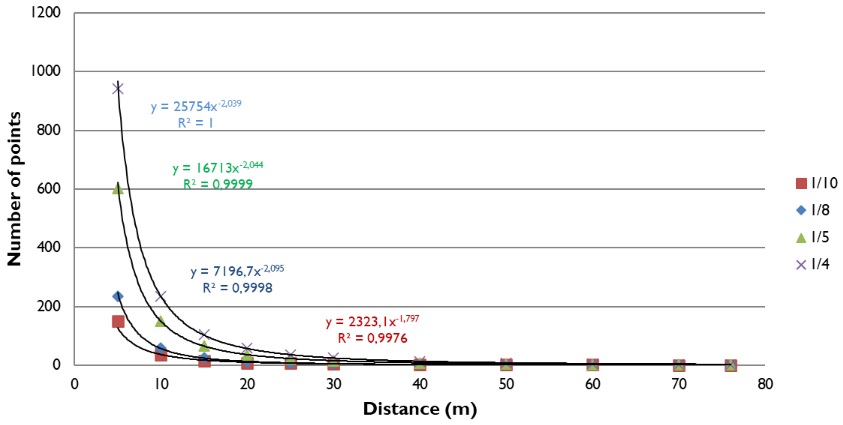
3.1.1. Calculation of the Theoretical Resolution

The theoretical resolution of the instrument is given by the expression $R\left(m\right)=\frac{2·\mathsf{\pi }}{RH·D}$ where R is the resolution in metres, RH is the horizontal resolution of the instrument, and D is the distance at which the resolution is to be calculated. The maximum resolution of the instrument is 40,000 × 20,000 points for the 360 × 320° at which the instrument is capable of recording data (

Table 5. Distance between points horizontally as a function of scanning resolution and object distance.

Resolution	1/1	1/2	1/4	1/5	1/8	1/10
Pts/400 g	40,000	20,000	10,000	8000	5000	4000
5	0.0008	0.0016	0.0031	0.0039	0.0063	0.0079
10	0.0016	0.0031	0.0063	0.0079	0.0126	0.0157
15	0.0024	0.0047	0.0094	0.0118	0.0188	0.0236
20	0.0031	0.0063	0.0126	0.0157	0.0251	0.0314
25	0.0039	0.0079	0.0157	0.0196	0.0314	0.0393
30	0.0047	0.0094	0.0188	0.0236	0.0377	0.0471
40	0.0063	0.0126	0.0251	0.0314	0.0503	0.0628
50	0.0079	0.0157	0.0314	0.0393	0.0628	0.0785
60	0.0094	0.0188	0.0377	0.0471	0.0754	0.0942
70	0.0110	0.0220	0.0440	0.0550	0.0880	0.1100
76	0.0119	0.0239	0.0478	0.0597	0.0955	0.1194

).

According to [24], it is advisable to have more than 55 points in order to have good position parameters of the sphere, (i.e., better in the order of a millimetre), which are to be used for high-precision network adjustment.

It is then possible to calculate the maximum number of theoretical points that will fall on a calibrated sphere, the radius of which is 0.0725 m. The results can be found in

Table 6. Theoretical points on a calibrated sphere as a function of resolution and distance.

Resolution Pts/400 g	1/1 40,000	1/2 20,000	1/4 10,000	1/5 8000	1/8 5000	1/10 4000
5	15,058	3765	941	602	235	151
10	3765	941	235	151	59	38
15	1673	418	105	67	26	17
20	941	235	59	38	15	9
25	602	151	38	24	9	6
30	418	105	26	17	7	4
40	235	59	15	9	4	2
50	151	38	9	6	2	2
60	105	26	7	4	2	1
70	77	19	5	3	1	1
80	59	14	3	2	1	1
90	46	11	2	1	0	0

, and from them it is possible to extract the fitting functions for the different resolutions relating the skimming distance to the number of points on the sphere, as seen in Figure 8, with these theoretical conclusions:

• For 1/10 resolution, high accuracy is only possible with scan distances less than 8.25 m, at best;
• If the scanning resolution is 1/8, it is not recommended to use distances greater than 10.35 m to calculate the least square spheres;
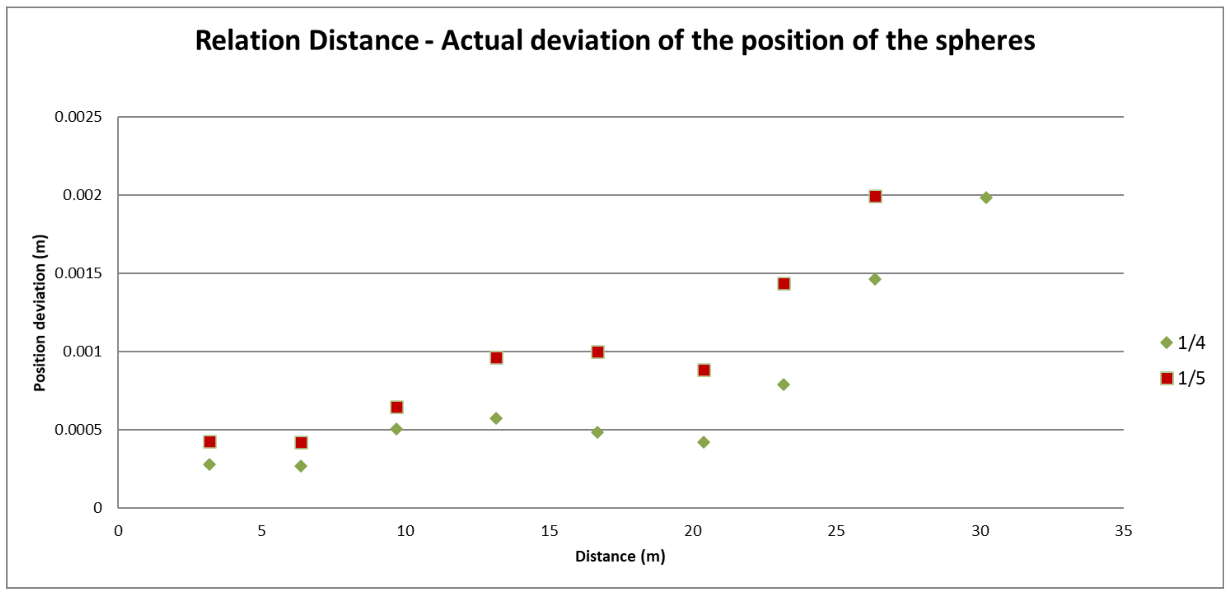
• A maximum of 16.55 m would be recommended for 1/5 resolutions;
• The theoretical maximum distance is 20.65 m for 1/4 scanning resolutions;
• Theoretically, with a resolution of 1/2, spheres up to 41.35 m could be recognised with guarantees;
• At maximum resolution, it should be possible to recognise a sphere over 82.7 m.

In terms of data volume, each pixel of the point cloud has to store the row, column, distance value, and digital level recorded by the laser beam. Each register is 16 bits, although the full depth of the data is not always exploited. The files have a 1024-byte header with the scan data, and each of the scan pixels occupies 8 bytes in its most basic form. Once processed, if exported, the first three values are replaced by the XYZ position of the point, and the digital level value resampled to 8 bits in grey (1 channel) or colour (3 channels) levels.

3.1.2. Data Capture for the Tests

A mixed field data capture campaign was designed, including both calibrated spheres and reference targets. The objective was to study the behaviour of the instrument against both types of references as a function of scanning resolution and distance.

On 18 April 2021, the measurements to carry out the normality tests were taken between 10:30 and 12:15. The environmental conditions were controlled at all times as described by [59,60,61,62,63], that is, temperature, pressure, and humidity values were recorded, and the experiment was carried out in a closed room to reduce the effects of interfering radiation. These records can be seen in

Table 7. Environmental conditions recorded during the normality test.

Time	Temperature (°C)	Pressure (hPa)	Humidity (%)
10:15	16.7	1003	74
10:30	16.9	1003	74
10:45	17.0	1003	74
10:00	17.2	1003	73
11:15	17.4	1004	73
11:30	17.6	1004	73
11:45	17.9	1004	73
12:00	18.1	1004	73
12:15	18.2	1004	74
12:30	18.4	1004	74

.

In the experiment carried out, first a scan was made at 1/10 of the maximum resolution of the instrument, so the laser could reach the optimum operating temperature. Then, the working area was delimited, and 7 scans were made at 1/4 resolution, and another 7 at 1/5 resolution. Finally, the position of the instrument was changed, and the experiment was repeated again at 1/5 and 1/4 resolution.

The tests carried out to analyse the behaviour of the scanner were analysed on the previous population of data.

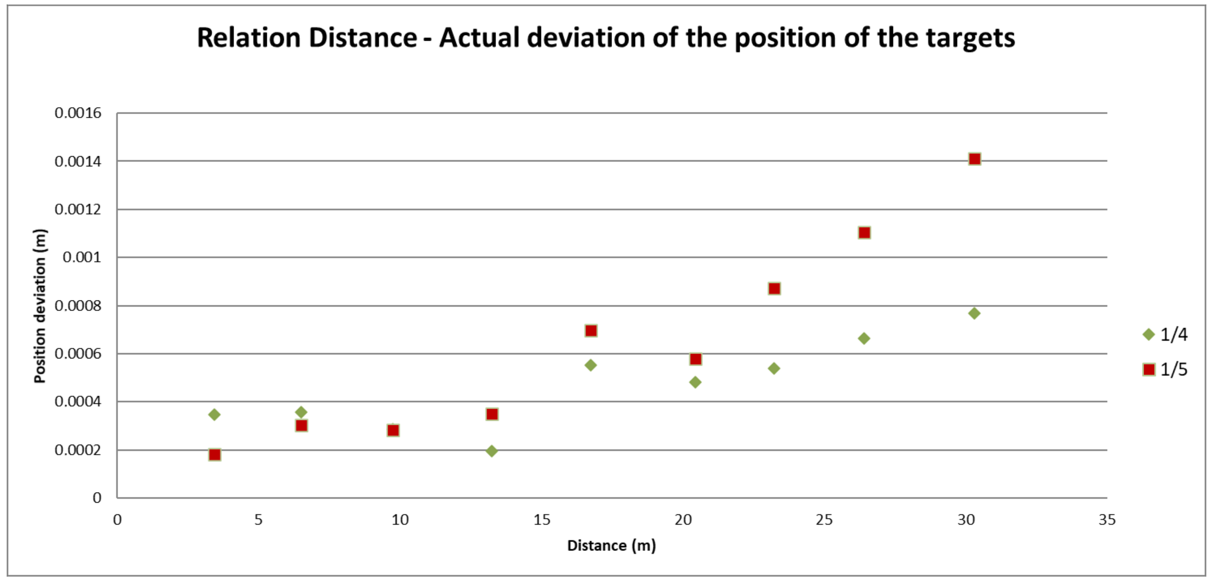
3.1.3. Measurement Accuracy Test

Applied Method

The aim of the experiment is to determine the actual deviation of the position of the modelled elements from, first, the measurements provided by the laser and, second, the elements modelled from them. For this purpose, the two types of target elements suitable for the laser (i.e., calibrated spheres and contrast targets) have been considered.

The test consisted of using the series of measurements described above to determine the most probable value and the standard deviation of these measurements, to compare the results provided by the manufacturer with real data.

For this purpose, the spheres and targets of each measurement were modelled and their positions determined. Then, the standard deviation of the values was calculated to determine the magnitude and dependence of this parameter as a function of distance.

Results Obtained from the Test

There were 9 samples for each distance and resolution. The results can be seen in Figure 9 and Figure 10.

Conclusions

From the results it can be concluded that with a resolution of 1/5 (Figure 9), it is possible to use spheres with good reliability up to 20 m, while with a resolution of 1/4 (Figure 10), it is possible to use them up to almost 25 m; above these thresholds a dilution of the accuracy would introduce more uncertainty into the network. The performance using targets in determining distances is better than spheres, provided that the information has been recorded by means of a normal shot. It can therefore be concluded that the laser detects coplanar elements better than spherical ones in an ideal case, although the latter are more practical in the field, as they always offer the same reliability, regardless of the position of the shot.

Both elements can be optimal for the calculation of high-precision 3D laser scanner grids.

3.1.4. Normality Test

To be able to affirm that the data fit theoretical models or known distributions, it is necessary to test the goodness of fit.

For each of the appropriate resolutions justified above, the theoretical probability for different distances between 3 and 27 m has been determined. From the technical specifications of the instrumentation, the reliability of an isolated point is 3 mm at 10 m, for high-reflectance values for both spheres and targets. Theoretically, the reliability of the elements modelled from these points according to [37], should be around 1.5 mm; this is why this value has been set as the confidence interval of the tests for both cases. Then, an empirical confidence interval has been calculated for each case to be able to know the degree to which it adjusts to the theoretical one.

Applied Method

The chi-square test is an example of a so-called statistical fit test, the purpose of which is to assess the goodness of fit of a set of data to a candidate distribution. It aims to accept or reject the following hypothesis: ‘The available data is a random sample from a distribution F_X(x)’.

The procedure for performing the chi-square test is:

• The range of values that the random variable of the distribution can take is divided into K adjacent intervals:

$$\left[a_0,a_1\right),\left[a_1,a_2\right),\dots ,\left[a_{k-1},a_k\right)$$

(196)

They can be $a_0=-\infty and{a}_k=\infty$

2.

Let $N_j$ be the number of values of the data we have that belong to the interval $\left[a_{j-1},a_j\right)$.

3.

Calculate the probability that the random variable of the candidate distribution $F_X\left(x\right)$ is in the interval $\left[a_{j-1},a_j\right)$.

Fx(x) is in the interval. For example, if it is a continuous distribution, this probability would be: Nj. In a continuous distribution, this probability would be:

$${{\displaystyle \int }}_{a_{j-1}}^{a_j}{f}_X\left(x\right)dx$$

(197)

$f_X\left(x\right)$ being the probability density function of the candidate distribution.

4.

The following test statistic is formed:

$$∆={\displaystyle \sum }_{j=1}^K\frac{{\left(N_j-N_p\right)}^2}{N_{p_j}}$$

(198)

If the fit is good, $∆$ will tend to take small values. We will reject the hypothesis of the candidate distribution if $∆$ takes ‘too large’ values. Note that to decide whether the values are ‘too large’, we need to set a threshold. To do so, we make use of the following property:

‘If the number of samples is sufficiently large, and the candidate distribution is appropriate, it tends to have a chi-square distribution of (K-1) degrees of freedom’.

In reality, the above statement is only strictly true if no parameters have to be estimated in the candidate distribution. If, to define the candidate distribution, some parameter has to be estimated (its mean, its variance, etc.) the number of degrees of freedom of the chi-square distribution is K-1-the number of parameters to be estimated from the data.

Therefore, if the candidate distribution is appropriate, we know the distribution of the parameter. If the candidate distribution is suitable, the value of the parameter $∆$ will tend to be small, and if it is not suitable, it will tend to be large.

A reasonable way to set a decision threshold would be:

‘Reject the candidate distribution if $∆>{\mathrm{\chi }}_{gdl,\alpha }^2$ being ${\mathrm{\chi }}_{gdl,\alpha }^2$ the value that in the chi-square distribution of gdl degrees of freedom leaves a probability mass of a above’.

Note that a, called the significance level, represents the probability of being wrong if the candidate distribution is appropriate, and it will be set to a small value (typically, 0.1, 0.05, or 0.01).

It is very important to bear in mind that the test is subject to error. We have just seen that it is possible to be wrong even if the hypothesis about the candidate distribution is true, because we can be unlucky enough to have large values for $∆$ that would, in any case, happen with probability. This would happen with low probability (0.1, 0.05, or 0.01, as we have just seen). Likewise, we could also err on the side of deciding that the candidate distribution is the right one even if it is not true, because the values of $∆$ could turn out to be small. The test is based on the reasonable assumption that if the candidate distribution is not the right one, the values of $∆$ will tend to be above the threshold ${\mathrm{\chi }}_{gdl,\alpha }^2$.

Results Obtained from the Test

Table 8. Normality test (${\mathrm{\chi }}^2$ ) for spheres and targets at 1/4 and 1/5 resolutions with a confidence interval of 1.5 mm. Calculation of the empirical confidence interval (in m) for each case.

	Confidence Interval at 1.5 mm				Empiric Confidence Interval
	${\mathit{\chi }}^2\mathbf{at}1/5$	Out of Range	${\mathit{\chi }}^2\mathbf{at}1/4$	Out of Range	Empiric Conf. Interval 1/5	${\mathit{\chi }}^2\mathbf{at}1/5$	Empiric Conf. Interval 1/4	${\mathit{\chi }}^2\mathbf{at}1/4$
Sphere 1	0.1823	0	0.6192	0	0.00035	0.7166	0.00037	0.7118
Sphere 2	0.0056	0	0.1371	0	0.00053	0.2627	0.00025	0.5308
Sphere 3	0.3849	0	0.1793	0	0.00032	0.3636	0.00067	0.2295
Sphere 4	0.1735	0	0.2388	0	0.00067	0.2809	0.00056	0.6710
Sphere 5	0.4130	0	0.9993	0	0.00071	0.2241	0.00128	0.7716
Sphere 6	0.2013	0	0.4106	1	0.00090	0.2129	0.00116	0.2754
Sphere 7	0.7345	0	0.6390	1	0.00113	0.3011	0.00109	0.3011
Sphere 8	0.7749	1	0.6117	0	0.00150	0.7823	0.00126	0.2530
Target 1	0.0008	0	0.1665	0	0.00021	0.8476	0.00037	0.2440
Target 2	0.0076	0	0.3475	0	0.00023	0.3709	0.00054	0.2278
Target 3	0.0581	0	0.0081	0	0.00033	0.0604	0.00027	0.2553
Target 4	0.1366	0	0.0100	0	0.00036	0.3702	0.00021	0.7815
Target 5	0.0131	0	0.4957	0	0.00067	0.7934	0.00039	0.9690
Target 6	0.3546	0	0.4134	0	0.00060	0.4936	0.00048	0.0944
Target 7	0.0077	0	0.1608	0	0.00058	0.7777	0.00101	0.0876
Target 8	0.8822	0	0.6536	0	0.00041	0.9789	0.00055	0.7992

shows the results obtained from applying a confidence interval of 15 mm to the tests in both cases; it also shows the calculations of the empirical confidence interval from the measured samples for each of the two cases. It can also be seen that some measurements are out of range when the theoretical confidence interval is applied.

Conclusions

Table 8 shows that all values are well below the calculated ${\mathrm{\chi }}^2$, which for two degrees of freedom and 95% confidence is 5.9914, so it can be stated that the measurements follow a normal distribution and can therefore be used for high-precision net observations.

There have been measurements that have been slightly outside the confidence intervals only when the element to be modelled has been spheres; this has been produced by the tail effect produced at the edges, which produces a reduction in accuracy at these points, as seen in Figure 11. Appropriate edge filtering reduces these effects, although sometimes, when the filtering is very restrictive, it can reduce the operating range due to the large information it removes. For the experiment, soft filtering has been applied.

From the present test it can be concluded that both the instrumentation used and the reference elements are suitable for the observation of high precision 3D laser scanner networks.

3.1.5. Conclusion on Fitness

The existence of redundant observations in a system means that from a mathematical viewpoint, no solution exactly fulfils the relationships established by these redundancies, and thus several solutions are obtained, even if only some observations are processed. The high accuracy and reliability of some current 3D laser scanner models has made it possible to develop networks for fitting the scans together.

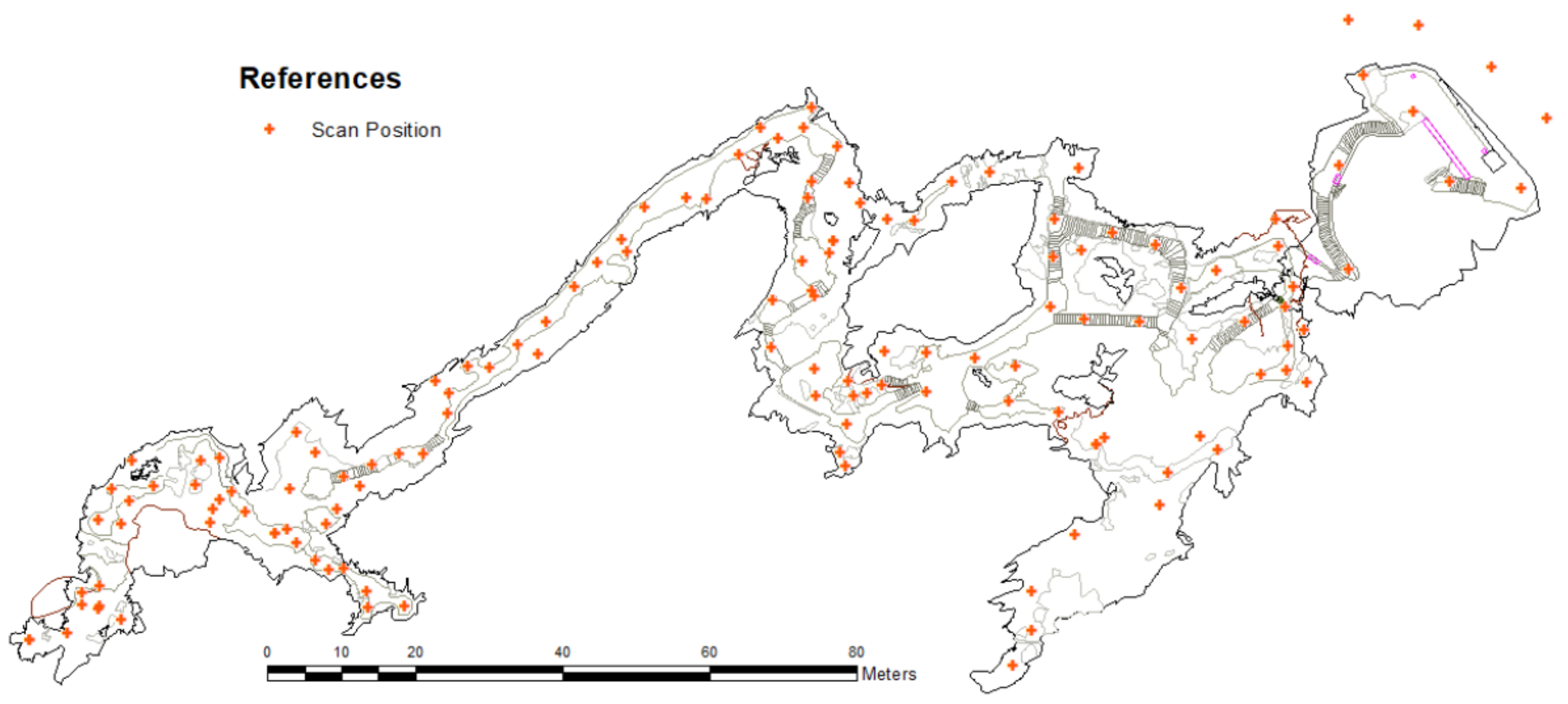
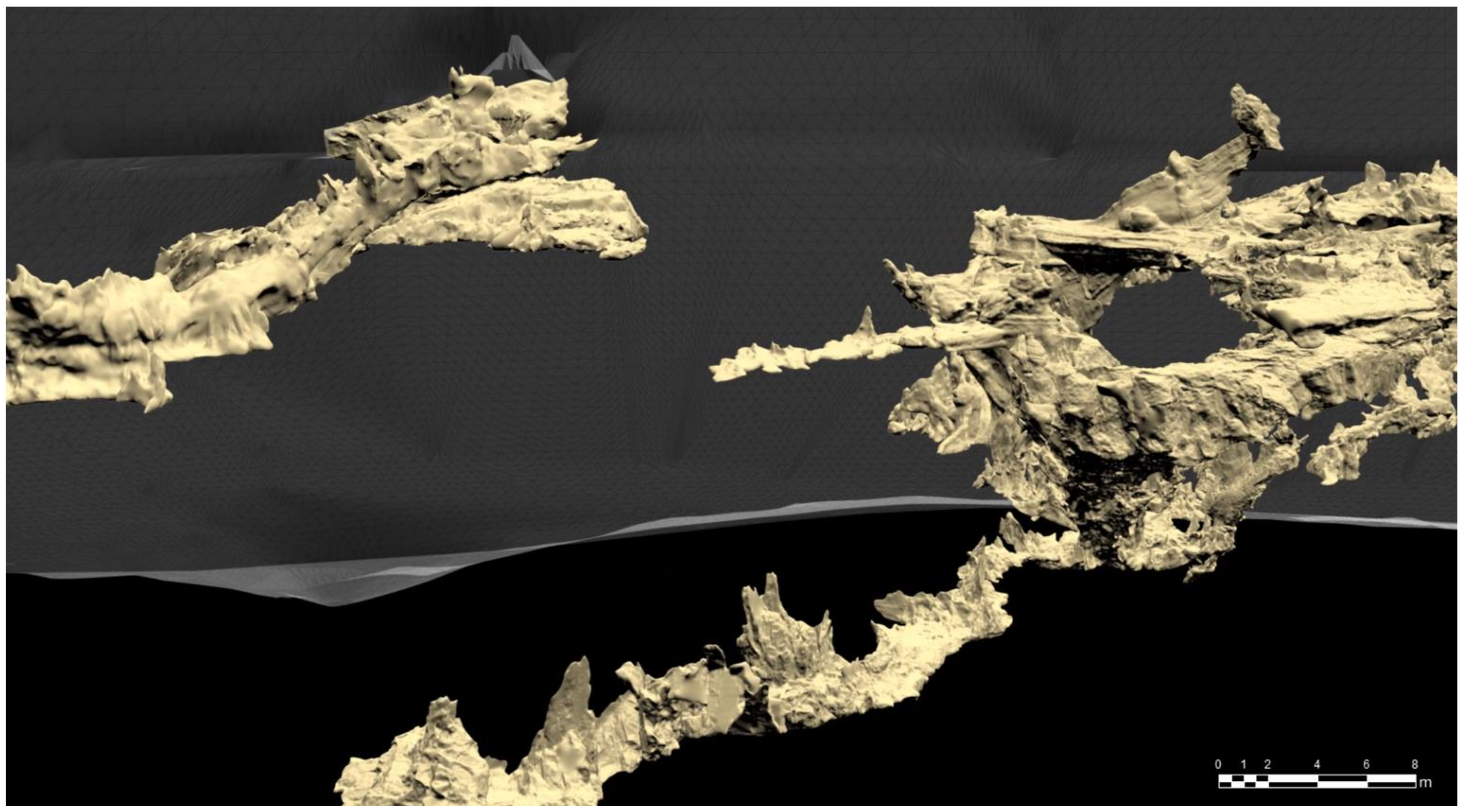
3.2. Practical Case: Cave Adjustment

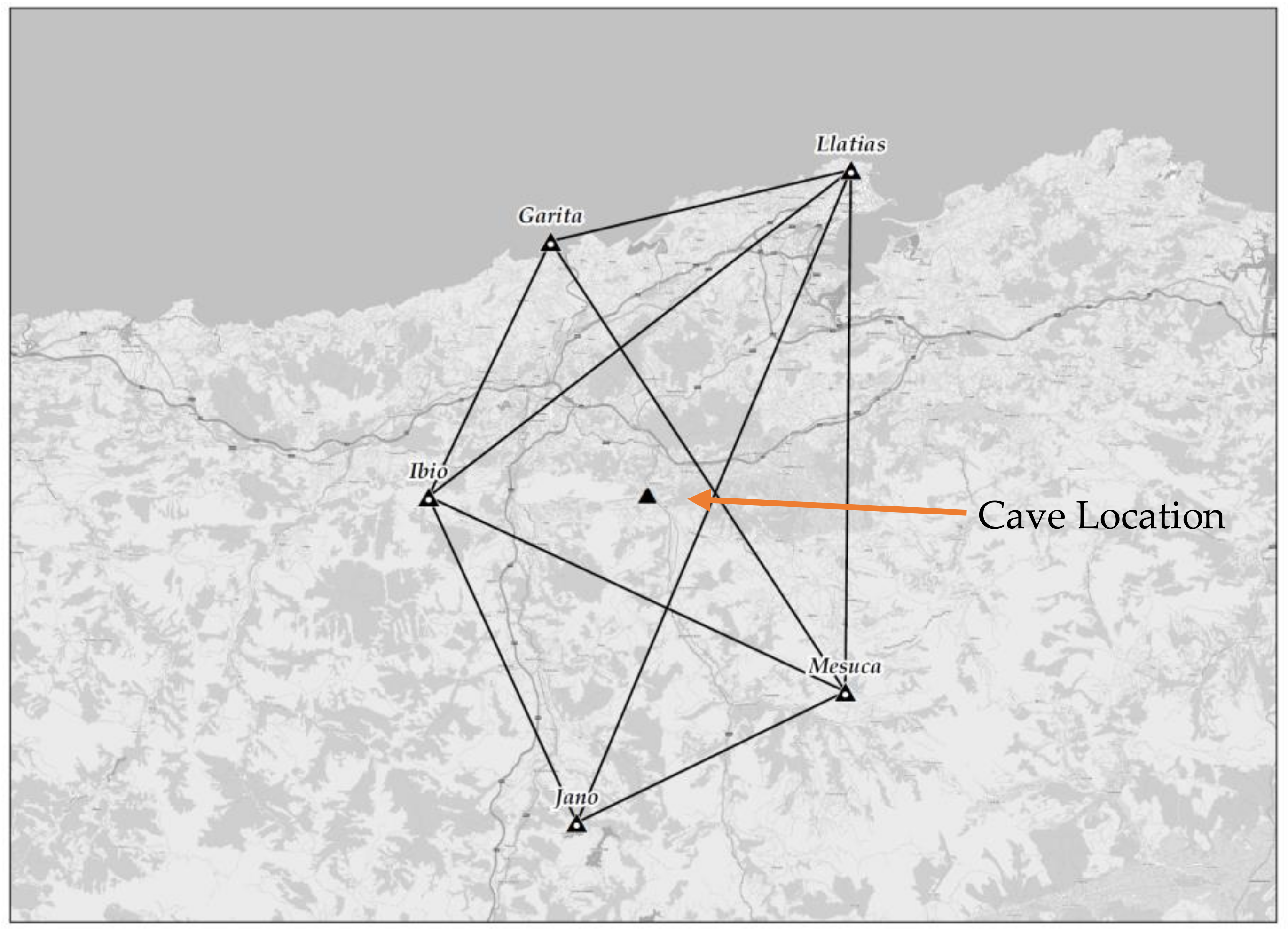
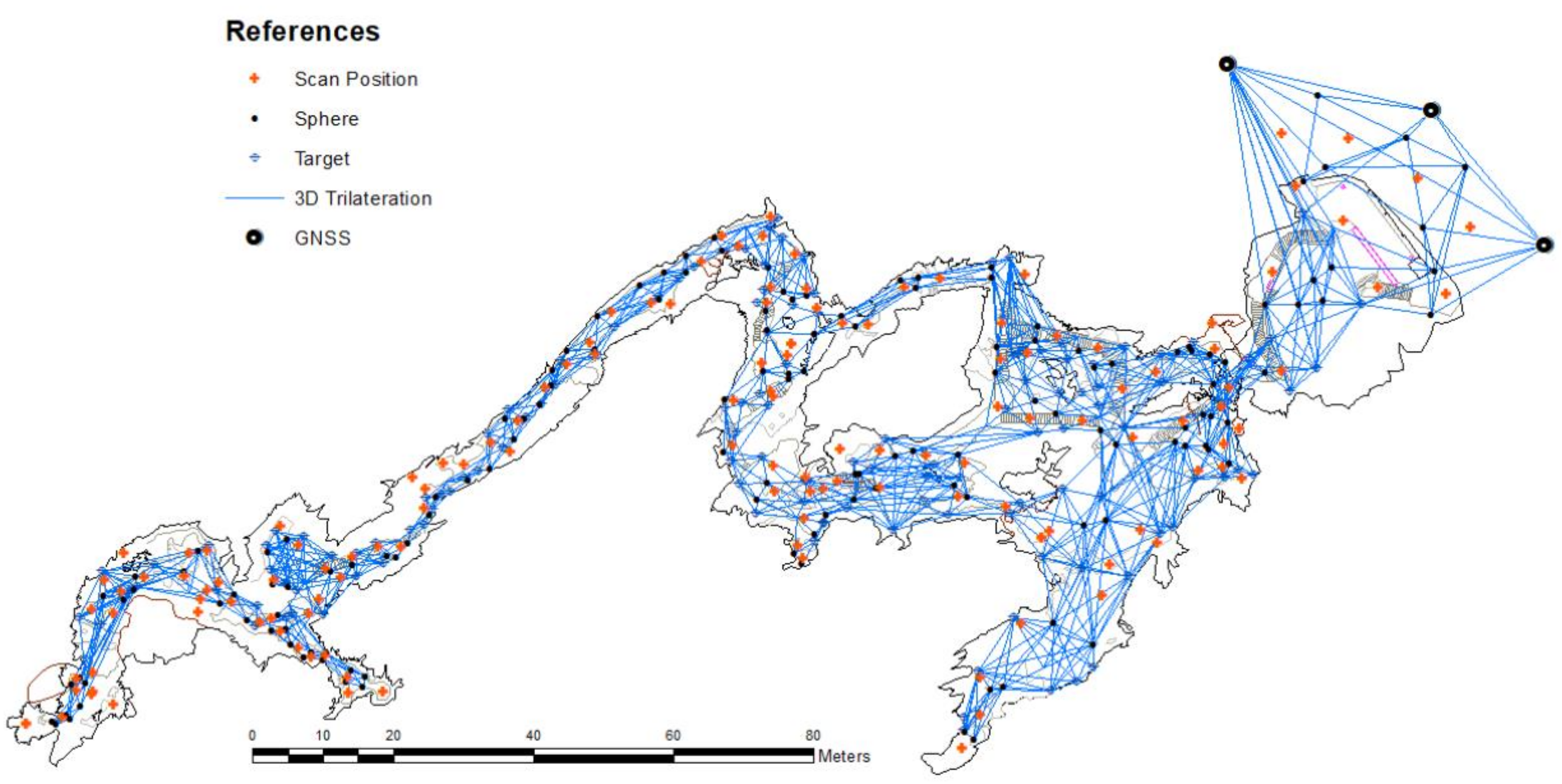
3.2.1. Global Navigation Satellite Systems (GNSS)

In our case, three sensors were used simultaneously in relative positioning, which enables more than one baseline to be determined during each observing session. After the first observing session, additional points are interconnected in the survey by moving the receivers to nearby stations. In this procedure, at least one receiver is left on one of the occupied stations. By employing this technique, a network of interconnected points can be created, as shown in Figure 12. In this figure, “Ibio” (station A) and “Mesuca” (station B) are control stations, and stations “Jano” (station C), “Garita” (station D), “Llatias” (station E), and “Cave Location”(station E) are points of unknown position. Creation of such networks is a common procedure employed in GPS relative positioning work.

In GPS surveying work where the observations are made using carrier phase observations, there are two stages where least squares adjustment is applied. The first is in processing the redundant observations to obtain the adjusted baseline components (ΔX, ΔY, ΔZ), and the second is in adjusting networks of stations wherein the baseline components have been observed.

The software Leica Geo Office was used to process observed phase changes to form the differencing observation equations, perform the least squares adjustment, and output the adjusted baseline vector components.

The software provided the covariance matrix, which expresses the correlation between the ΔX, ΔY, and ΔZ components of each baseline. This is a proprietary software that cannot be included herein.

The second stage where least squares is employed in processing GPS observations is in adjusting baseline vector components in networks. This adjustment is made after the least squares adjustment of the carrier-phase observations is completed. It is also done in the X_e, Y_e, Z_e geocentric coordinate system. In network adjustments, the goal is to make all X coordinates (and all X-coordinate differences) consistent throughout the figure. The same objective applies for all Y and Z coordinates.

This consists of two control stations and four stations whose coordinates are to be determined. A summary of the baseline observations obtained from the least squares adjustment of carrier-phase measurements for this figure is given, and the covariance matrix elements listed in the table are used for weighting the observations.

Three GNSS points of known coordinates were observed and adjusted as described in Section 2.5.2 in the exterior of the cave.

3.2.2. Observation Generation from Scan Points

The cave is about 400 m long and is divided into different spaces in rooms, corridors, galleries, and roundabouts. Throughout its extension, this cavern contains a large number of animal figures, such as aurochs, goats, deer, hinds, reindeers, horses, and so on [64]. In order to scan the cave, 133 scans (Figure 13) were necessary along the entire route. All the following data is contained in the .FWS file and is extracted thanks to FARO Open SDK.

In total, 135 checkerboards and 135 calibrated spheres were radiated from the scans (Figure 14). An ASCII text file with the observation data was generated with the following format:

Name_Of_Reference, Scan_Position, X_coordinate, Y_coordinate, Z_coordinate, Radius, number_of_points used to calculate the reference, normal_transversal_deviation, normal_longitudinal_deviation, and distance to scan point.

The file contains 873 lines corresponding to each reference taken from any of 145 scan positions.

3.2.3. D Trilateration

The calibrated spheres and checkerboards are calculated from the point cloud of each station. These references are represented by red lines in Figure 15c, where each reference is linked to the station where it was taken. Then, the 3D trilateration sides (Figure 15d) are generated by performing a weighted average with their equals recorded at other stations (i.e., spheres 3 and 5 generate a side recorded from 4 positions). The number of times the distance between two references have been measured affects the variance of the observable, the study of the normality, and also the error.

Once the observation data is available, the file is sorted to create the sides of the 3D trilateration by using a weighted average of the observations, based on the number of times it has been measured and the reliability of the measurements (Figure 16). From the previous file, 171 trilateration sides were created and adjusted following the general adjustment model of Section 2.5.1.

As commented, 3 GNSS points (see Figure 16) were observed and adjusted to be used as points of known coordinates in the trilateration network adjustment. The constraint equations were added as described in Section 2.5.3.

The weighted average of each 3D trilateration side and the statistics were calculated according to Section 2.5.5.

The result is a file containing:

Reference_Name_1; Reference_Type_1; Reference_Name_2; Reference_Type_2; Mean_Value; Standard_Deviation_Estimation;

The least squares adjustment was calculated by setting a maximum correctness threshold of 0.2 mm, and after 12 iterations the solution converged.

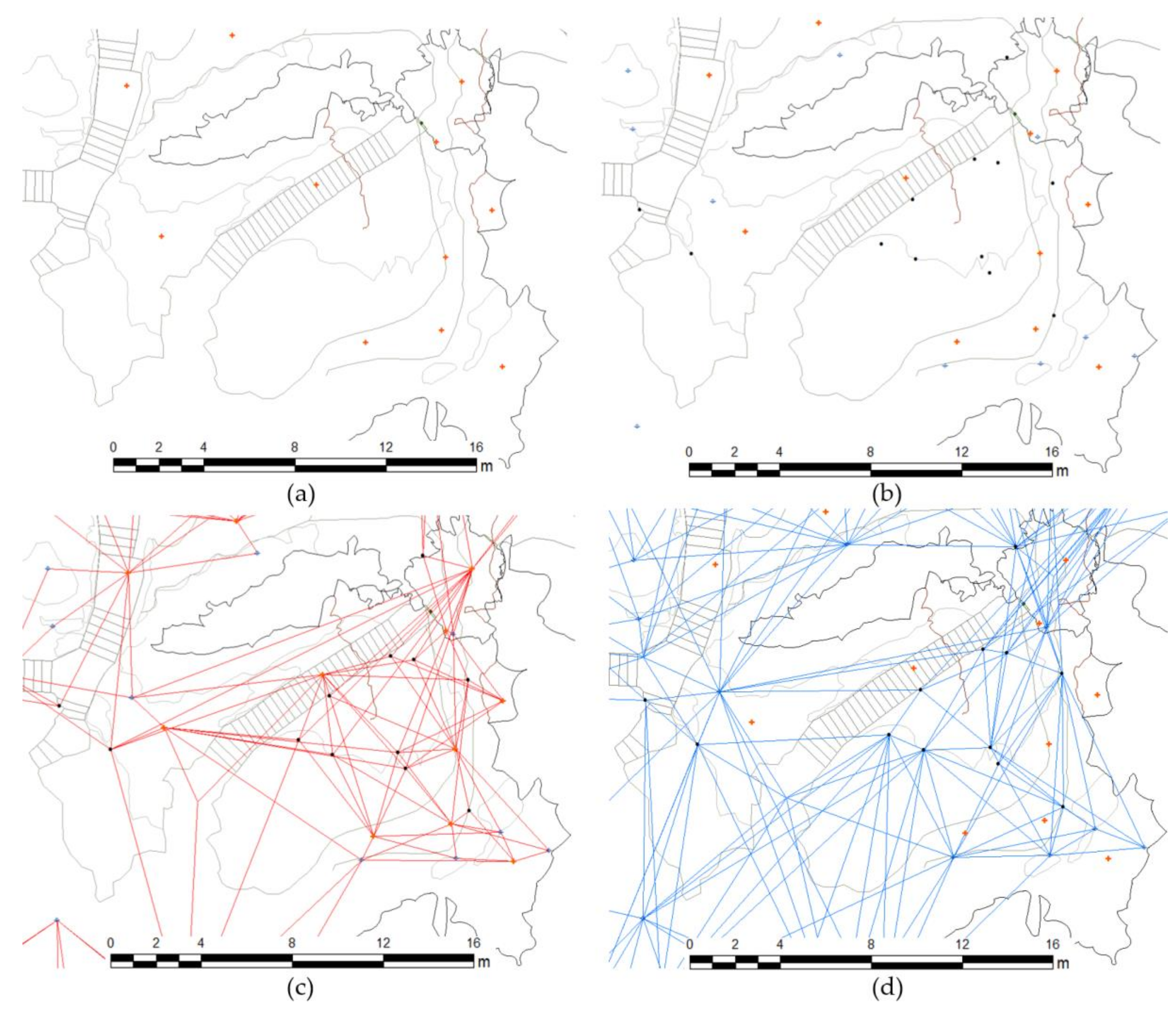
3.2.4. Measures of Accuracy and Reliability

The datum problem tries to determine the optimal fixed parameter definition for each network. This part deals with how the quality of the observations affects the fitting results through the network geometry (accuracy) and how the network reacts to small deviations of the observations (reliability) or robustness of the network, as described in Section 2.5.7.

Absolute Standard Ellipses

The standard deviations of the coordinates of a network point have been calculated from the variance-covariance matrix of the parameters. The values indicate the error estimate in the directions.

The values corresponding to the major and minor semi-axes of the standard error ellipse corresponding to a probability of 39.4% have been obtained, and later, the expansion factors corresponding to a 95% probability level calculated.

The result is a list as:

Name_Of_Ellipse, X_coordinate, Y_coordinate, Z_coordinate, Semi-major axis, Semi-minor axis, Orientation.

Relative Standard Ellipses

Relative standard error ellipses have been calculated for a pair of points on a planimetric grid.

The result is a list as:

Name_Of_Ellipse, Reference_1, Reference_2, X_coordinate, Y_coordinate, Z_coordinate, Semi-major axis, Semi-minor axis, Orientation

Uncertainty Hyper-Enclosures

Despite being rigorous and clear (see Section 2.5.7), it is necessary to establish simplification hypotheses since it is impractical or simply inapplicable in interpreting results in specific cases. In our case, the simplification consisted in calculating a section of the error hypercylinder by planes generated by pairs of reference axes and a file with the hyperellispsoid axes generated. The results have been stored in an ASCII file.

3.2.5. Post-Adjustment Statistical Analysis

To control the observations, some post-adjustment tests (see Section 2.5.8) were run, such as the chi-square test, to control whether the a posteriori reference variance ${\mathrm{\sigma }}_0^2$ is compatible with the reference variance a priori. The data snooping and Pope’s test was used to localise gross error and eliminate them.

4. Discussion

The paper shows a methodology to adjust, following the traditional topo-geodetic methods, 3DTLS data by modelling references such as calibrated spheres and checkerboards to generate a 3D trilateration network from them.

The method tries to find the function that best fits the measured data, considering not only that the measurements made in the field are not perfect, but that each one of them has a different deviation depending on the adjustment of each reference, so they have to be weighted accordingly.

The methodology improves the accuracy in cartography and models of caves and contributes to showing the relationship between different caves within the same karst (Figure 17).

The observation, calculation, and least squares compensation of a network such as the one in question is a centuries-old doctrine and praxis not yet surpassed in scientific rigor by point cloud adjustment methods, which generally behave like a “black box”, offering no parameters of adjustment reliability. The research and technology of commercial brands has been geared more towards achieving high practical yields than towards improving achievable accuracies.

The presented method makes it possible to achieve adjusted results with sub-millimeter error figures, although to progress, a detailed review of the classical algorithms and methods of observation and calculation is necessary.

It is necessary that the observables of the adjustment are normal independent random variables, and it is also necessary that they pass the normality test.

The integration of 3DTLS and GNSS permits a rapid, accurate, and reliable recording of complex features such as the caves or cavities [2,65,66]. The information can be used to derive cartography such as floor plans, contour lines, longitudinal and cross sections, three-dimensional analysis, scenarios for virtual reality [67], or just the base for hyperspectral studios [3,4,64,68].

The accuracy of the new models permits cave managers to aid in decision making, especially when parameters are interrelated and used to generate prediction models such as hydrochemical, microbiological, climatic, geotechnical, or faunal models, which require measuring multiple parameters, many of which are highly correlated and perform predictive behavioural processes within a knowledge-based system [1].

5. Conclusions

Prehistoric art is an extraordinary manifestation that has documented in great detail and precision facts and animal species that coexisted with humans in Palaeolithic times, through representations of engravings and pigment painting on the surfaces of caves [69]. Such cavities are usually part of karst systems, which evolve over time and also include microhabitats in which animal and plant communities develop [70,71]. At a certain point, man took advantage of some of these cavities to inhabit them, occupying these microhabitats, and in such a way he became integrated and formed an active part of the evolution of the karst system itself, altering it with contributions of organic matter and fire The rediscovery of these caves by modern man, with his admiration for prehistoric culture and his “right” to contemplate it, transmit it, exploit it, and protect it, makes it necessary to analyse the sustainability of such a precious resource.

Traditionally, for prehistoric sites and caves—although they have been something special and fragile, and measures have been taken to guarantee their conservation—the need to cater to an increasing number of visitors meant that, especially between the 1950s and 1970s, the sites were adapted for tourism, which, with the massive influx of visitors, helped to disrupt the natural balance that had allowed such fragile heritage to endure for such a long time.

The locations where rock art exists constitute a complex natural system [72], in which, besides the interactions between the rock, water, and air, other factors intervene, such as the cohesion of the pigments used, their composition, the technique used in the engravings, the existence of living communities on or in the supporting rock and their characteristics, and the incidence of anthropic actions (Figure 18).

The combination of geomatics techniques such as remote sensing, photogrammetry, and geographic information systems allows the development of an operational methodology to quantify, at a relatively low cost, actions aimed at carrying out sustainable heritage management [73,74]. For proper heritage management, it is essential to have good systematised and permanently updated information, which lacks many points of interest of heritage. These methods are also characterised by being the most efficient in terms of documentation and therefore have the least impact on the cave, which favours the sustainability of the cave.

Inside the caves, where GNSS is not available, in order to carry out a topographic survey, points with known coordinates are needed on which to base oneself directly or indirectly. These points are called vertices, and all of them together are called the topographic network or basic network.

The purpose of the observations can be to obtain the coordinates of these points or to create a cartographic reference system for the development of cartographic or photogrammetric work.

In a project, a distinction is usually made between the planimetric and the altimetric basic network. Planimetric networks have the purpose of establishing geographical latitude and longitude (λ, φ) or Cartesian (X, Y) coordinates of the points. Altimetric grids determine the third coordinate, the height on the geoid. The vertices may be the same, but the situational conditions are completely different, and this means that the points that form both networks in the same work do not always coincide.

The method takes advantage of co-registered and geo-referenced point clouds by any algorithm, such as ICP, which does not consider the source model’s error or total least squares algorithms based on the Gauss–Helmert model, to derive accuracy and reliability measurements and post-adjustment statistical analysis, which is used to calculate the planimetric and altimetric coordinates of the reference frame materialised by spheres and checkerboards to generate a 3D trilateration network from them.

The proposed method has made it possible to generate data to revise the classical error figures in several aspects, especially by not taking into account more than the central band of the symmetrical ${\sigma }_{xx}$ matrix. More rigorous error figures have been obtained, where the complete matrix, in all its elements, is considered. The new figures described as “vertex rosettes” and “correlated” also densify the specific error control points of the network.

In addition, an error figure has been established, represented by a straight elliptic hypercylinder, with n-d real and finite axes, which is an n-axis hyperellipsoid in the deterministic or bound network case.

All this information makes it possible to correlate information from different adjacent caves belonging to the same karst and to model parameters such a gaseous exchange, hydrological models, microbiological propagation, and weather—cases where distances between galleries must be calculated rigorously to achieve accurate results.

References

1. Ontañon, R.; Bayarri, V.; Herrera, J.; Gutierrez, R. The conservation of prehistoric caves in Cantabria, Spain. In The Conservation of Subterranean Cultural Heritage; CRC Press/Balkema: Boca Raton, FL, USA; Taylor & Francis Group: London, UK, 2014; ISBN 978-1-315-73997-7. [Google Scholar]
2. Bayarri-Cayón, V.; Castillo, E. Caracterización geométrica de elementos complejos mediante la integración de diferentes técnicas geomáticas. Resultados obtenidos en diferentes cuevas de la Cornisa Cantábrica. In Proceedings of the VIII Semana Geomática Internacional, Barcelona, Spain, 3–5 March 2009. [Google Scholar]
3. Bayarri, V. Algoritmos de Análisis de Imágenes Multiespectrales e Hiperespectrales para la Documentación e Interpretación del Arte Rupestre. Ph.D. Thesis, Universidad Nacional de Educación a Distancia, Madrid, Spain, May 2020. Available online: http://e-spacio.uned.es/fez/view/tesisuned:ED-Pg-TecInd-Vbayarri (accessed on 25 July 2021).
4. Matsuoka, M.T.; Rofatto, V.F.; Klein, I.; Roberto Veronez, M.; da Silveira, L.G., Jr.; Neto, J.B.S.; Alves, A.C.R. Control Points Selection Based on Maximum External Reliability for Designing Geodetic Networks. Appl. Sci. 2020, 10, 687. [Google Scholar] [CrossRef] [Green Version]
5. Baarda, W. S-transformations and criterion matrices. Publ. Geod. New Ser. 1973, 5, 168. [Google Scholar]
6. Grafarend, E.W. Optimization of Geodetic Networks. Can. Surv. 1974, 28, 716. [Google Scholar] [CrossRef]
7. Klein, I.; Matsuoka, M.T.; Guzatto, M.P.; Nievinski, F.G.; Veronez, M.R.; Rofatto, V.F. A new relationship between the quality criteria for geodetic networks. J. Geod. 2019, 93, 529. [Google Scholar] [CrossRef]
8. Seemkooei, A.A. Comparison of reliability and geometrical strength criteria in geodetic networks. J. Geod. 2001, 75, 227–233. [Google Scholar] [CrossRef]
9. Seemkooei, A.A. Strategy for Designing Geodetic Network with High Reliability and Geometrical Strength. J. Surv. Eng. 2001, 127, 104–117. [Google Scholar] [CrossRef] [Green Version]
10. Teunissen, P.J.G. Quality Control in Geodetic Networks. In Optimization and Design of Geodetic Networks; Grafarend, E.W., Sansò, F., Eds.; Springer: Berlin/Heidelberg, Germany, 1985; pp. 526–547. [Google Scholar]
11. Gargula, T. Adjustment of an Integrated Geodetic Network Composed of GNSS Vectors and Classical Terrestrial Linear Pseudo-Observations. Appl. Sci. 2021, 11, 4352. [Google Scholar] [CrossRef]
12. Vanícek, P.; Craymer, M.R.; Krakiwsky, E.J. Robustness analysis of geodetic horizontal networks. J. Geod. 2001, 75, 199–209. [Google Scholar] [CrossRef]
13. Amiri-Simkooei, A. A new method for second order design of geodetic networks: Aiming at high reliability. Surv. Rev. 2004, 37, 552–560. [Google Scholar] [CrossRef]
14. Amiri-Simkooei, A.; Sharifi, M.A. Approach for Equivalent Accuracy Design of Different Types of Observations. J. Surv. Eng. 2004, 130, 1–5. [Google Scholar] [CrossRef] [Green Version]
15. Hekimoglu, S.; Erenoglu, R.C.; Sanli, D.U.; Erdogan, B. Detecting Configuration Weaknesses in Geodetic Networks. Surv. Rev. 2011, 43, 713–730. [Google Scholar] [CrossRef]
16. Hekimoglu, S.; Erdogan, B. New Median Approach to Define Configuration Weakness of Deformation Networks. J. Surv. Eng. 2012, 138, 101–108. [Google Scholar] [CrossRef]
17. Besl, P.J.; Mckay, N.D. A method for registration of 3-D shapes. IEEE Trans. Pattern Anal. Mach. Intell. 1992, 14, 239–256. [Google Scholar] [CrossRef]
18. Fritsch, D.; Wagner, J.F.; Ceranski, B.; Simon, S.; Niklaus, M.; Zhan, K.; Mammadov, G. Making Historical Gyroscopes Alive—2D and 3D Preservations by Sensor Fusion and Open Data Access. Sensors 2021, 21, 957. [Google Scholar] [CrossRef]
19. Koch, K.R. Parameter Estimation and Hypothesis Testing in Linear Models; Springer: Berlin/Heidelberg, Germany, 1999; 333p. [Google Scholar]
20. Bayarri, V.; Sebastián, M.A.; Ripoll, S. Hyperspectral Imaging Techniques for the Study, Conservation and Management of Rock Art. Appl. Sci. 2019, 9, 5011. [Google Scholar] [CrossRef] [Green Version]
21. Alcalde Del Río, H.; Breuil, H.; Sierra, L. Les Cavernes de la Région Cantabrique (Espagne); Impr. V A. Chêne: Rabat, Monaco, 1911. [Google Scholar]
22. Espeleo Club de Gràcia. El Sector Oriental del Massís del Dobra (Puente Viesgo); Exploracions Nº 6; Espeleo Club de Gràcia: Barcelona, Spain, 1982. [Google Scholar]
23. Ripoll, S.; Bayarri, V.; Muñoz, F.J.; Latova, J.; Gutiérrez, R.; Pecci, H. El arte rupestre de la cueva de El Castillo (Puente Viesgo, Cantabria): Unas reflexiones metodológicas y una propuesta cronológica. In Capítulo en Libro Cien Años de Arte Rupestre Paleolítico Centenario del Descubrimiento de la Cueva de la Peña de Candamo (1914–2014); Ediciones Universidad de Salamanca: Salamanca, Spain, 2014; ISBN 978-84-9012-480-2. [Google Scholar]
24. FARO. FARO Laser Scanner Focus 3D X 330 TEchnical Datasheet. Available online: https://faro.app.box.com/s/nn8swfhtez68lo88uhp6u8bchdfl1ay9/file/441669546444 (accessed on 11 June 2021).
25. Chueca Pazos, M.; Herráez Boquera, J.; Berné Valero, J.L. Redes Topográficas y Locales. Microgeodesia; Paraninfo: Madrid, Spain, 1996. [Google Scholar]
26. Hogg, R.V.; Johannes, L. Applied Statistics for Engineers and Physical Scientists; Macmillan: New York, NY, USA, 1992. [Google Scholar]
27. Mikhail, E.M.; Gordon, G. Analysis /& Adjustment of Survey Measurements; Van Nostrand Reinhold Company: New York, NY, USA, 1981. [Google Scholar]
28. Ghilani, C.D. Statistics and Adjustments Explained, Part 3: Error Propagation. Surv. Land Inf. Sci. 2004, 64, 29–33. [Google Scholar]
29. Jorge, R.; Eduardo, B. Medical image segmentation, volume representation and registration using spheres in the geometric algebra framework. Pattern Recogn. 2007, 40, 171–188. [Google Scholar] [CrossRef]
30. Franaszek, M.; Cheok, G.; Witzgall, C. Fast automatic registration of range images from 3D imaging systems using sphere targets. Automat. Constr. 2009, 18, 265–274. [Google Scholar] [CrossRef]
31. Wang, Y.; Shi, H.; Zhang, Y.; Zhang, D. Automatic registration of laser point cloud using precisely located sphere targets. J. Appl. Remote Sens. 2014, 8, 083588. [Google Scholar] [CrossRef]
32. Press, W.H.; Flannery, B.P.; Teukolsky, S.A.; Vetterling, W.T. Numerical Recipes in C: The Art of Scientific Computing; Cambridge University Press: Cambridge, UK, 1988. [Google Scholar]
33. Rabbani, T. Automatic Reconstruction of Industrial Installations Using Point Clouds and Images; Publications on Geodesy 62; Netherlands Geodetic Commission: Delft, The Netherlands, 2006. [Google Scholar]
34. Eberly, D. 3D Game Engine Design: A Practical Approach to Real- Time Computer Graphics; Academic Press: Cambridge, MA, USA, 2001. [Google Scholar]
35. Box, G.E.P.; Draper, N.R. Empirical Model-Building and Response Surface; John Wiley & Sons: Hoboken, NJ, USA, 1986. [Google Scholar]
36. Boro, K.R.; Bielajew, A.F. Quadplot: A Programme to Plot Quadric Surfaces; Technical Report NRCC/PIRS-0491; Institute for National Measurement Standards, National Research Council of Cañada: Ottawa, ON, Cañada, 1995. [Google Scholar]
37. Bookstein, F. Fitting Conic Sections to Scattered Data. Comput. Graph. Image Process. 1979, 9, 56–71. [Google Scholar] [CrossRef]
38. Leick, A. GPS Satellite Surveying, 2nd. ed.; John Wiley & Sons: New York, NY, USA, 1995. [Google Scholar]
39. Mikhail, E.M.; Ackermann, F. Observations and Least Squares; Harper & Row Publishers: New York, NY, USA, 1976. [Google Scholar]
40. Cooper, M.A.R. Control Survegs in Civil Engineering; Coliins Profesional and Technical Books; Nichols Pub. Co: New York, NY, USA, 1987. [Google Scholar]
41. Wolf, P.R.; Charles, D.G. Adjustment Computations: Statistics and Least Squares in Surveying and GIS; Wiley Interscience: Hoboken, NJ, USA, 1997. [Google Scholar]
42. Harvey, B.R. Practical Least Squares and Statistics for Surveyors; En Monograph 13 (University of New South Wales, ed.); Kensington: Sidney, Australia, 1991. [Google Scholar]
43. Chueca Pazos, M.; Anquela Julián, A.B.; Baselga Moreno, S. Diseño de Redes y Control de Deformaciones. Los Problemas del da Tum y Principal de Diseño; Editorial Universidad Politécnica de Valencia: Valencia, Spain, 2007. [Google Scholar]
44. Strang, G.; Kai, B. Linear Algebra, Geodesy and GPS; Wellesley Cambridge Press: Cambridge, UK, 1997. [Google Scholar]
45. Caspary, W.F. Monograph 11: Concepts of Network and Deformation Analysis; The University of New South Wales: Sydney, Australia, 1988. [Google Scholar]
46. Kuang, S. Geodetic Network Analysis and Optimal Design. Concepts and Applications; Ann Arbor Press Inc.: Chelsea, MI, USA, 1996. [Google Scholar]
47. Dracup, J.F. Squares Adjustment by the Method of Observation Equations with Accuracy Estimates. Surv. Land Inf. Sci. 1994, 55, 2. [Google Scholar]
48. De La Fuente, J.L.O. Técnicas de Cálculo Para Sistemas de Ecuaciones, Programación Lineal y Programación Entera; Reverte S.A.: Barcelona, Spain, 1998. [Google Scholar]
49. Harvey, B. Practical Least Squares and Statistics for Surveyors; School of Surveying, University of New South Wales: Sydney, Australia, 1994. [Google Scholar]
50. Gruëndig, L. Special Adjustment tools for Surveying Networks. In Papers for the Precise Engineering and Deformation Surveys Workshop; University of Calgary. Publ.: Calgary, AB, Canada, 1985; Volume 60004. [Google Scholar]
51. Haim, B.P.; David, S. Relative error of geodetic Networks. J. Surv. Eng. ASCE 1985, 111. [Google Scholar] [CrossRef]
52. Leick, A. Adjustment Computations; University of Maine: Orono, ME, USA, 1980. [Google Scholar]
53. Alian, A.L. Practical Surveging and Computations; Butter-Worth/Heinemann: Oxford, UK, 1993. [Google Scholar]
54. Dewitt, B.A. An Efficient Memory Paging Scheme for Least Squares Adjustment of Horizontal Surveys. Surv. Land Inf. Sci. 1994, 54, 147–156. [Google Scholar]
55. Pope, A.J. The Statistics of Residuals and the Detection of Outliers; NOAA Technical Report, NOS 65, NGS 1; National Geodetic Survey: Rockville, MD, USA, 1976. [Google Scholar]
56. Barnes, D. GPS Status and Modernization. Presentation at Munich Satellite Navigation Summit 2019. Available online: https://www.gps.gov/cgsic/international/2019/munich/barnes.pdf (accessed on 28 July 2021).
57. Zrinjski, M.; Barković, Đ.; Matika, K. Razvoj i modernizacija GNSS-a. Geod. List 2019, 73, 45–65. Available online: https://hrcak.srce.hr/218855 (accessed on 16 July 2021).
58. Hein, G.W. Status, perspectives and trends of satellite navigation. Satell. Navig. 2020, 1, 22. [Google Scholar] [CrossRef]
59. Cross, P.A. Advanced Least Squares Applied to Positionjixing; Working papers; Univrsity of East London: London, UK, 1983. [Google Scholar]
60. Rüeger, J.M. Electronic Distance Measurement: An Introduction; Springer: Berlin/Heidelberg, Germany, 1990. [Google Scholar]
61. Gielsdorf, F.; Rietdorf, A.; Gruendig, L. A Concept for the calibration of terrestrial láser scanners. In Proceedings of the FIG Working Week, Athens, Greece, 22–27 May 2004; In CD-ROM. Available online: https://m.fig.net/resources/proceedings/fig_proceedings/athens/papers/pdf/ts_26_2_gielsdorf_etal_ppt.pdf (accessed on 28 July 2021).
62. Boehler, W.; Bordas, M.; Marbs, A. Investigating Láser Scanner Accuracy. In Proceedings of the XIXth CIPA Sgmposium, Working Group 6, Antalya, Turkey, 30 September–4 October 2003. [Google Scholar]
63. Amiri Parían, J.; Grün, A. Integrated láser scanner and intensity image calibration and accuracy assessment. Int. Arch. Photogramm. Remóte Sens. Spat. Inf. Sci. 2005, 36, 18–23. [Google Scholar]
64. Bayarri, V.; Castillo, E.; Ripoll, S.; Sebastián, M.A. Improved Application of Hyperspectral Analysis to Rock Art Panels from El Castillo Cave (Spain). Appl. Sci. 2021, 11, 1292. [Google Scholar] [CrossRef]
65. Ripoll, S.; Bayarri, V.; Muñoz, F.J.; Ortega, R.; Castillo, E.; Latova, J.; Herrera, J.; Moreno-Salinas, D.; Martín, I. Hands Stencils in El Castillo Cave (Puente Viesgo, Cantabria, Spain). An Interdisciplinary Study. Proc. Prehist. Soc. 2021, 1–21. [Google Scholar] [CrossRef]
66. Bayarri-Cayón, V.; Latova, J.; Castillo, E.; Lasheras, J.A.; De Las Heras, C.; Prada, A. Nueva ortoimagen verdadera del Techo de Polícromos de la Cueva de Altamira, ARKEOS | perspectivas em diálogo, nº 37. In XIX International Rock Art Conference IFRAO 2015. Symbols in the Landscape: Rock Art and Its Context. Conference Proceedings; Instituto Terra e Memória: Tomar, Portugal, 2015; pp. 2308–2320. [Google Scholar]
67. Barrera, S.; Otaola, A.; Bayarri-Cayón, V. Explotación Turística no Intrusita de la Cueva de Santimamiñe (Vizcaya) Mediante Realidad Virtual. II Congreso Español de Cuevas Turísticas; Asociación de Cuevas Turísticas Española: Madrid, Spain, 2009; pp. 359–371. [Google Scholar]
68. Bayarri, V.; Latova, J.; Castillo, E.; Lasheras, J.A.; De Las Heras, C.; Prada, A. Nueva documentación y estudio del arte empleando técnicas hiperespectrales en la Cueva de Altamira. ARKEOS | perspectivas em diálogo, nº 37. In XIX International Rock Art Conference IFRAO 2015. Symbols in the Landscape: Rock Art and Its Context. Conference Proceedings; Instituto Terra e Memória: Tomar, Portugal, 2015. [Google Scholar]
69. Muñoz, E.; Ontañón, R.; Bayarri-Cayón, V.; Montes, R.; Morlote, J.M.; Bayarri-Cayón, V.; Herrera, J.; Gómez, A.J.G. La Cueva de Cueto Grande (Miengo, Cantabria-España). Un Nuevo Conjunto de Grabados Paleolíticos en la Región Cantábrica., in: ARKEOS | Perspectivas Em Diálogo, No 37. Symbols in the Landscape: Rock Art and Its Context. Presented at the XIX International Rock Art Conference IFRAO. 2015, pp. 945–967. Available online: http://www.apheleiaproject.org/apheleia/Articles/COLLADO%20et%20al%202015%20Symbols%20in%20the%20Landscape%20Rock%20Art%20and%20its%20Context.%20Arkeos%2037.pdf (accessed on 28 July 2021).
70. Ontañón, R.; Bayarri, V.; Castillo, E.; Montes, R.; Morlote, J.M.; Muñoz, E.; Palacio, E. New discoveries of pre-Magdalenian cave art in the central area of the Cantabrian region (Spain). J. Archaeol. Sci. Rep. 2019, 28, 102020. [Google Scholar] [CrossRef]
71. Montes, R.; Bayarri-Cayón, V.; Muñoz, E.; Morlote, J.M.; Ontañon, R. Avance al Estudio del Registro Gráfico Paleolítico de la Cueva de Solviejo (Voto, Cantabria, España). Cuadernos de Arte Prehistórico Número 3. 2017. Available online: https://cuadernosdearteprehistorico.com/index.php/cdap/article/view/21 (accessed on 28 July 2021).
72. Ripoll-López, S.; Bayarri-Cayón, V.; Latova Fernández-Luna, J.; Herrera-López, J.; Benavides Miguel, M. El Proyecto de Investigación: Elaboración de una Sistema Gestor para la protección, puesta en valor y divulgación de Arte Rupestre y Estaciones Prehistóricas (SIGAREP I y II). X Jornadas de Patrimonio Arqueológico en la Comunidad de Madrid. Dirección General de Patrimonio Histórico. Museo Arqueológico Regional. Alcalá de Henares (Madrid). November 2014. Available online: https://www.researchgate.net/publication/283489912_El_Proyecto_de_Investigacion_Elaboracion_de_una_Sistema_Gestor_para_la_proteccion_puesta_en_valor_y_divulgacion_de_Arte_Rupestre_y_Estaciones_Prehistoricas_SIGAREP_I_y_II (accessed on 28 July 2021).
73. Hatzopoulos, J.; Stefanakis, D.; Georgopoulos, A.; Tapinaki, S.; Pantelis, V.; Liritzis, I. Use of various surveying technologies to 3d digital mapping and modeling of cultural heritage structures for maintenance and restoration purposes: The tholos in Delphi, Greece. Mediterr. Archaeol. Archaeom. 2017, 17, 311–336. [Google Scholar]
74. Jamhawi, M.; Alshawabkeh, Y.; Freewan, A.; Al-Gharaibeh, R. Combined Laser Scanner and Dense Stereo Matching Techniques For 3d Modelling Of Heritage Sites: Dar Es-Saraya Museum. Mediterr. Archaeol. Archaeom. 2016, 16, 185–192. [Google Scholar] [CrossRef]
Figure 1. Location map of El Castillo Cave. The cave is in Puente Viesgo, Cantabria, Spain [3].
Sustainability 13 13526 g001
Figure 2. (a) Plan of the El Castillo cave in Les cavernes de la région Cantabrique of 1911 [21] (b) Plant of the Espeleoclub de Gràcia of 1982 [22] (c) Plan of the present-day El Castillo cave [23] (d) Present-day 3D model of the cave.
Sustainability 13 13526 g002
Figure 3. Overall workflow.
Sustainability 13 13526 g003
Figure 4. Parameters of the sphere object models. The sphere is parametrised by its centre c = ( c x , c y , c z ) and its radius.
Sustainability 13 13526 g004
Figure 5. Approximate values realised by a quadric fit of the sphere.
Sustainability 13 13526 g005
Figure 6. Distance generation from four references.
Sustainability 13 13526 g006
Figure 7. Observation of a distance.
Sustainability 13 13526 g007
Figure 8. Theoretical relationship between resolution, number of points on a sphere, and scanning distance.
Sustainability 13 13526 g008
Figure 9. Relationship between distance and actual standard deviation of calibrated spheres at 1/4 and 1/5 resolutions.
Sustainability 13 13526 g009
Figure 10. Relationship between distance and actual standard deviation of targets at resolutions of 1/4 and 1/5.
Sustainability 13 13526 g010
Figure 11. Tail points produced by the edges of the spheres.
Sustainability 13 13526 g011
Figure 12. GPS survey network.
Sustainability 13 13526 g012
Figure 13. Map of scan positions.
Sustainability 13 13526 g013
Figure 14. Map of scan positions (red cross), targets (blue target), and calibrated spheres (black sphere).
Sustainability 13 13526 g014
Figure 15. Detail of the entrance of the cave (a) position of the scans (red cross); (b) position of the targets (blue target) and calibrated spheres (black sphere) taken from each scan; (c) representation of elements taken from each scan, where each sphere or target is linked to the scan position from which it was recorded; (d) representation of 3D trilateration generated between captured references, where elements from each scan position are trilaterated between them.
Sustainability 13 13526 g015
Figure 16. 3D trilateration network generated from observations.
Sustainability 13 13526 g016
Figure 17. Karst of Mount Castillo. The models represent the adjusted cave and permit one to appreciate in detail the spatial relationship between them.
Sustainability 13 13526 g017
Figure 18. Biotic and abiotic elements of the karst system [3].
Sustainability 13 13526 g018