How Does Travel Demand Follow the Change in Infrastructure? Multiple-Year Eigenvector Centrality Analysis

Abstract

The road network is one of the most permanent elements of the physical structure of cities, and the long-term impacts should be considered for effective and efficient road network improvement. It is therefore important to catch up on how the road will be used after construction. However, we do not have much knowledge on the pattern and time lag in the change process of travel demand and supply in the real situation. To explore such changes, this study proposes to evaluate a network with eigenvector centrality (EC) measures that can evaluate the importance of nodes in a network. We believe the analysis based on topological properties by the graph theory is suitable to verify the evolution of road networks. This study analysed long-term changes over 20 years in an actual city to understand the impact of road network improvements. The EC analysis with the weights of traffic indices obtained from survey data evaluates the connectivity of road services on the supply side, and traffic concentration on the demand side.

1. Introduction

Recently, the impact of natural disasters has increased owing to climate and social changes. It is important to increase societal resilience to such disasters. In emergency situations, road networks are more important than other modes of transport [1] because of their extensive coverage and ability to maintain connections between urban centres. Public transport is likely to be out of service during a disaster, and people will be more dependent on the road network. Therefore, the improvement of a robust road network is necessary. Based on the idea of coping with disasters and other unpredictable events that should be added to planning and design for sustainability, the effects of actual bridge collapse accidents were evaluated for urban street topology using space syntax theory [2]. Changes in the configuration and topology of road networks can either enhance or impair resilience. However, road construction is expensive and time-consuming. To ensure the comprehensive and stable supply performance of roads, effective and efficient investments are needed.

Let us begin with what will change when the road network is improved. Transportation networks and land use patterns may influence each other over time mutually. Changes to transportation networks, such as the construction of a new link or expansion of an existing one, eventually influence the location of investment inland, which in turn influences the demand for travel to and from a particular location. There exists plenty of research discussing land use transport interaction (LUTI), and Wegener [3] and Iacono et al. [4] review important theoretical frameworks to represent the complex relationship between transportation and land use. The system dynamic approach to identify cause and effect in dynamic change processes has been developed based on the pioneering research activities by Forrester [5]. System dynamic models focus on accessibility to make the land attractive in terms of work, transportation, residence and business. Moreover, all the elements are interacting, and a change in any one thing affects the whole.

Many equilibrium problems and simulation analyses have been studied as traditional system dynamic approaches. Equilibrium problems require high computational loads. In addition, the results of LUTI simulations may vary significantly depending on many parameters. It is difficult to ensure the accuracy of predicting the future and collecting information to set these parameters. Furthermore, these previous studies have considered changes in the time span and delays in the reaction; however, few discussions are made on an adequate time interval of simulation. For example, behaviour changes gradually as new roads are constructed and the accessibility is improved, but little attention has been given to finding out how long a time span the change follows. We would like to examine how many lags there are from the supply and demand side for actual road improvement cases based on a simple topological approach of road networks. Thus, this study evaluates the road networks based on a topological approach to understand the impact of long-term road improvements.

This study verifies the impact of road network improvement by using eigenvector centrality analysis, which is one of the topological-based approaches. This measure identifies sets of nodes in a directed network that are strongly connected to each other and, conversely, sets of nodes that are weakly connected to each other. An advantage of this approach is that the EC measure indicates the strength of the connection of one node to its adjacent nodes while considering their strengths of connections. Topological-based approaches evaluate the network in terms of inherent structure, and moreover, the weights can be selected according to what you want to evaluate. In addition to the changes in road network topology over a long period, the effects of the weights are also considered in the evaluation. The values that characterise transport supply and demand are set as weights in this study. One of the contributions of this study is to analyse the actual changes in road network improvement performed in the target area. Two hypotheses can be made about the actual road construction. The first is that the road network is designed to meet the current traffic demand, and the second is that the transport demands are induced so as to meet the supply level of the road network. This study empirically tests these hypotheses in terms of long-term relationships between traffic demand and supply. The result of the empirical analysis will enhance knowledge on the response to road improvement, which is useful for road network improvement planning. Eigenvector centrality can be used to express infrastructure improvement both in the immediate vicinity and in the surrounding area. Supply-side analysis was used to evaluate the connectivity of road services, and demand-side analysis was used to evaluate traffic concentration. We analysed long-term changes in eigenvector centrality values to understand the impact of road network improvements.

This paper is organised as follows. Section 2 summarises the literature review and the definition of relevant indicators. Section 3 presents the definition of eigenvector centrality measures. In addition, the weight settings for the demand side and the supply side are introduced. Section 4 summarises the long-term improvements of road networks by construction history and survey data in Gifu Prefecture, Japan from 1985 to 2024 (including planning). Section 5 shows the results of eigenvector centrality measures with different weights by the supply side and demand side. Section 6 discusses the relationships between evaluations of the supply side and demand side in the long term. The last section concludes our works.

2. Literature Review

2.1. Land Use and Transportation Interaction Model

Research discussing urban modelling often emphasises the importance of modelling different phenomena with some time scales. As Wegener [3] suggests, a transport network is one of the most permanent elements of the physical structure of cities, and large infrastructure projects require a decade or more, and once in place, are rarely abandoned. Such changes occur very slowly. The changes in workplaces and housings or land use may change slowly in accordance with the network change, which is often evaluated by distances or travel time. Given the fixed origin–destination patterns of travel, the travel, mode, or route to use can be changed instantaneously in accordance with congestion and so on. Wegener [6] and Hunt et al. [7] describe exclusive modelling techniques for interpreting the land use and transportation interaction. Especially, Wegener [6] identified the urban change process in eight types of major urban subsystems, which are classified by the speed of change. Moreover, the characteristics of each model are organised, and they classify which model corresponds to which speed of change. Most LUTI models consider such changes in different time spans by taking account of time lags or delays due to the complex superposition of slow and fast processes of urban development.

We briefly describe the LUTI model of the process by which dynamic analysis becomes common. There are many review papers on the detailed development of the LUTI model (e.g., [8]). The LUTI model was initially developed based on urban economic modellings such as positive theory by Alonso [9] and normative theory by Herbert and Stevens [10]. However, statistic models have a discrepancy with reality in that all events are adjusted simultaneously. Therefore, Fujita [11] developed the model from static to dynamic by integrating these urban economic models and the theoretical land use model. As for the equilibrium models, Anas [12] incorporated employment and population into the Lowry model [13], developed the urban equilibrium model and considered the consistency with the network equilibrium model. Based on this theory, many empirical studies have been conducted [14]. In recent years, analysis using microsimulation models has increased. Microsimulation models usually employ an agent-based approach that represents the behaviour of disaggregated agents. The LUTE model [15] is an agent-based microsimulation model that considers the change processes in the eight types of major urban subsystems. People, households and companies are described as agents, and long-term events such as residential place choice and car ownership are considered. The objective of this simulation model is to analyse a broad range of transportation, housing and other urban policies. As for a study examining the long-term effects of transportation system improvement, Musolino [16] proposed a spatial accounting LUTI model. The effect of introducing a sustainable mobility system was simulated in terms of activity location, land price, travel demand and transport accessibility before and after the introduction of that system. The simulation models for long-term evaluations tend to be mainly concerned with parameter settings, and this model by Musolino [16] also describes parameter calibration as one of the challenges.

These simulation models are easy to understand and have many components that can be adjusted; therefore, they can reproduce many cases. On the contrary, extensive data requirements for calibration and excessively long computing time are significant issues of the implementation of microsimulations [17]. These limitations are the reasons that agent-based simulation models are not suitable for a long-term planning decision. As for empirical studies of long-term land use and road improvement, Patarasuk and Binford [18] verified the relationship between significant road improvement and land-cover change in Thailand between 1989 and 2006. The results show that in areas with a well-developed road network, there was a large shift from forest to agriculture, and also a shift from food crop to cash crop. The empirical analysis in Thailand shows that road network improvement changes livelihoods and leads to economic development. On the other hand, the optimal solution to road network improvement tends to be the construction of roads adjacent to high-demand places. However, this increases the disparity between cities and rural areas and thus is not suitable for sustainable development. Santos et al. [19] selected three equity indices with different perspectives: accessibility to less attractive places, the dispersion of accessibility to all places and the dispersion of accessibility among all places and places in the same region. The results of incorporating them into the design model confirm that different results can be obtained depending on the equity indicators chosen. These previous studies show that changes in supply performance have the potential to produce a significant impact on demand. Conversely, the characteristics of the demand may determine the plan of improvement. How to improve the road network in the long-term perspective should be carefully discussed.

This study attempts to evaluate the effect of road improvement by a topological-based approach that represents simple properties, which is suitable for long-term analysis. We verify the relationship between demand and supply perspectives by focusing on actual road improvement histories.

2.2. Network Analysis by Topological Approach

Early research on topological transportation networks was conducted on simple network and geometric properties due to limited data and calculation resources. Garrison [20] firstly introduced graph theory in geographical analysis, and Garrison and Marble [21] and Kansky [22] proposed the traditional connectivity indices for plane graphs, $\alpha$-index, $\mathsf{\beta }$-index and $\gamma$-index. Haggett and Chorley [23] summarised theoretical concepts and network topological models of traffic patterns and geography. At that time, many empirical studies were conducted using traditional connectivity indices (Medvedkov [24] and Royaltey et al. [25]). In an extended study related to these, Xie and Levinson [26] proposed three complementary measures: heterogeneity of the road network, connection patterns and continuity that indicates the inconvenience of transferring between different levels. The analysis of the connection pattern, however, only focuses on the topological properties of roads in plane graph. Quantification metrics show the properties of complex network structures and may be useful to investigate the evolution of networks in space and time.

With the improvement of observation technology, traffic flow models have been developed, and traffic assignment and equilibrium models based on demand data have become active. We do not describe them in detail here. In recent years, network topological analysis methods based on graph theory have been focused on as an evaluation method for large-scale networks that are difficult to apply high load computation and simulation to. Since the 2000s, the topological approach to infrastructure networks can be categorised into two primary methods: network efficiency and centrality measures. Latora and Marchiori [27] introduced an efficiency indicator that defined the average of the reciprocal of the minimum path length across all node pairs. Moreover, a global efficiency has been proposed that shows how direct the connections between all node pairs are by comparing the Euclidean distance with the shortest network distance. These network efficiency indices are highly related to the characteristics of small-world networks. Centrality is a value that indicates which node or link is “central” in the network, and there are various definitions of centrality. The idea of centrality was firstly applied in social networks to understand human community structure in small groups [28]. Subsequently, this concept has been adopted in various fields such as diffusions of infectious diseases, information and communication systems, economics, engineering and so on [29].

Empirical studies by combining traditional connectivity indices ($\alpha$-index, $\beta$-index and $\gamma$-index) with network efficiency and centrality measures have been researched. Morgado and Costa [30] compared simple topological properties from ancient corridor roads to recent motorway road networks by using traditional connectivity indices. Additionally, the changes in the airplane network were verified by using the accessibility index. They found a tendency for connectivity to decline over time and then to recover again in long periods. Erath et al. [31] focused on the fact that network analysis is a method of measuring the growth of networks. The indices for plane graphs organised by Xie and Levinson [26], betweenness centrality and degree centrality were applied to roads, railways and population in Switzerland between 1950 and 2000 to understand the characteristics over time. In a similarly long-term performance, Casali and Heinimann [32] evaluated road network improvement in Zurich, Switzerland, for changes between 1955 and 2012. They investigated how the development of geographical properties and road network topology affects the distribution of centrality. The results analysed by three types of betweenness centrality, which were weighted according to distance, population and undirected, showed the most important nodes becoming even more important in 2012. However, the traditional connectivity indices showed no change over time because indices depend on the average degree of networks.

For road network evaluations by centrality measures as the main indicator, Lämmer et al. [33] showed that the frequency distribution of the betweenness centrality based on travel time follows the power law. This means that the number of important nodes with high betweenness centrality values is limited in the whole network, indicating a clear hierarchical order of the roads. Duan et al. [34] evaluated the stability of urban road network robustness by three different granularities, segment stroke and community level, using the degree and betweenness centrality. They found that the level of robustness varies by observation granularity and that centrality measures can effectively represent the robustness of the network. Jiang et al. [35] adopted a special notation method where each node represents a street name and links are created if there is an intersection between two streets. Three centrality measures are applied to characterise the urban areas and identify important streets: degree, closeness and betweenness centrality. In an example of using multiple centrality indices, Crucitti et al. [36] evaluated the road networks of 18 cities by degree, closeness, betweenness, straightness and information centrality. The distribution of closeness, betweenness and straightness centrality is similar in several cities, however, information centrality is differently distributed in planned and self-organised cities, exponential for planned cities and power-law for self-organised ones. Porta and Latora [37] proposed the Multiple Centrality Assessment based on a theory of network efficiency and some centrality measures, and indicated the spatial characteristics and “skeleton” of an urban structure by centrality analysis.

The equations and definitions of some representative centrality measures are introduced here.

Table 1. Representative centrality measures.

Centrality Measures	Formulation	Definition
Degree Centrality	$x_i=k_i$	The number of links connected to the node
Closeness Centrality	$x_i=\frac{N}{{\sum }_j{d}_{ij}}$	A reciprocal of the average distance from a node to all other nodes using the shortest path
Betweenness Centrality	$x_i=\sum _{st}\frac{n_{st}^i}{g_{st}}$	The extent to which a node lies on the shortest paths between other nodes
Eigenvector Centrality	$x_i=\sum _j{a}_{ij}{x}_j$	The importance of a node in a network is increased by having connections to other nodes that are themselves important

shows the formulation of four centrality measures with reference to Newman [28]. $x_i$ represents a centrality value of node $i$, $k_i$: the degree of node $i$, $N$: the number of nodes, $d_{ij}$: distance between node $i$ and node $j$, $n_{st}^i$: the number of shortest paths from $s$ to $t$ that traverse node $i$, $g_{st}$: the total number of shortest paths from $s$ to $t$ and $a_{ij}$: an element of the adjacency matrix $A$. The most straightforward concept of centrality is degree centrality, which is a node-based measure defined as the number of links incident upon the node [38]. This is defined as the sum of each row or column in the adjacency matrix representing network connections. An extension of degree centrality is eigenvector centrality [39]. Degree centrality only represents the effect of directly connected nodes, whereas eigenvector centrality considers the dissemination effect of connectivity among nodes in the network. Relative scores are increased for nodes with connections to high-scoring nodes. Closeness centrality evaluates how close a node is to all other nodes [40]. To obtain closeness centrality, we need to calculate the shortest distance between all node pairs. Betweenness centrality counts the number of shortest paths traversing a node [41]. As is the case with closeness centrality, the shortest distance path search is required for all node pairs, and the set of nodes included in each shortest path should be recorded to calculate betweenness centrality. Many other centrality measures have also been defined, such as Katz centrality [42] and Page Rank centrality [43].

As shown in the literature review above, betweenness and closeness centrality, which have the concept of a path between node pairs, are often applied in road networks. These measures require the enumeration of the paths between all node pairs or a search for the shortest path. On the other hand, eigenvector centrality does not specify a path and, thus, each node affects all of its neighbours simultaneously. Eigenvector centrality with a small computational load is, therefore, suitable for evaluating large-scale networks, which is one of the advantages of a topological-based approach. While eigenvector centrality is ideally suited for “influence type” processes that simultaneously assume multiple “paths” such as the spread of trends and information, there is a limitation that values are often extremely connected in a few large hubs in the network. Martin et al. [44] attempted to relax this problem by changing the expression of the adjacency matrix. However, road networks in general have a limited degree due to spatial constraints. It is difficult to concentrate the traffic function in a specific location because of the properties of traffic capacity and volume. Hence, the degree distribution of the road network does not have a power law [45].

Eigenvector centrality (EC) is often used to evaluate social networks. For example, in researching professionals’ relationships using the co-author data of published papers, EC is more suited than other centrality measures for identifying the critical author. The reason is that authors are highly qualified, have relationships with other highly qualified researchers and then are likely to publish high-quality papers [46]. Many other kinds of social networks have been conceptually or empirically analysed in terms of what type of centrality measures are most suitable (e.g., [47,48]). In contrast to these, much less research has been conducted on the application of EC to infrastructure network systems. Ando et al. [49] indicated the method of capacity-weighted EC to evaluate the connectivity of road networks. Moreover, the comparison between EC and other centrality measures revealed that there is a correlation between capacity-weighted EC and closeness centrality. This is an advantage for EC that does not require a search for the shortest path or route enumeration. This analysis is based on actual road network data; therefore, the usefulness of EC for road networks has been confirmed.

3. Methodology

3.1. Eigenvector Centrality

Here, we will look at the mathematical characteristics of EC. Let

$$A\mathit{x}=\lambda \mathit{x}$$

(1)

where $\mathit{x}$ is an eigenvector, $\lambda$ is an eigenvalue and $A$ is a weighted adjacency matrix with element:

$$a_{ij}=\{\begin{array}{c}{w}_e if e=\left(i,j\right)\in \mathit{e}\\ 0 \mathrm{otherwise}\end{array}$$

(2)

$w_e$ is the weight of the link $e$ connecting node $i$ and $j$. Let us consider a transportation network $G=\left(\mathit{v},\mathit{e}, \mathit{w}\right)$, where $\mathit{v}$ is the set of nodes, $\mathit{e}$ is the set of links and $\mathit{w}$ is the vector of link weights. In this study, we are interested in asymmetric matrices because the weight of a link may differ with direction. Generally, a road network is strongly connected with bidirectional links in the network. Thus, its associated weighted adjacency matrix is irreducible. The concept of strong connectedness is closely related to the concept of matrix irreducibility. Proposition 1 and the following two definitions show their relationship. The following proposition and proof are mentioned in reference to Cheung et al. [50].

Definition 1.

A directed graph$G$is strongly connected if for any two distinct nodes$i$,$j$, there is a directed path of finite length that starts at$i$and ends at$j$. A directed graph$G$is weakly connected if it is not strongly connected, but when considering it as an undirected graph it is connected, i.e., for any two distinct nodes$i$,$j$, there is an undirected path of finite length that starts at$i$and ends at$j$.

Definition 2.

A non-negative square matrix$\mathbf{M}\in {ℝ}^{n\times n}$is irreducible if for any$i, j=1,2, \dots , n$, there exists a positive integer$k$such that${\left({\mathbf{M}}^k\right)}_{ij}>0$.

where$M$is a large positive number,$ℝ$is set of non-negative real numbers and$n=\left|V\right|$.

Proposition 1.

Suppose$G$is a directed graph with n nodes and$\mathbf{A}\in {ℝ}^{n\times n}$is the associated non-negative weighted adjacency matrix. Then,$\mathbf{A}$is irreducible if and only if its associated graph is strongly connected.

Proof of Proposition 1.

Since $G$ is a graph with $n$ nodes, then $A$ is irreducible if and only if all entries of $\sum _{k=1}^n{A}^k$ are greater than 0. The proposition is established via the following reduction. Let $Q$ be the matrix obtained from $A$ by replacing all non-zero entries by 1. Then, the following statements are trivial:

• $A$ is irreducible if and only if $Q$ is irreducible;
• ${\left(\sum _{k=1}^n{A}^k\right)}_{ij}$ is positive if and only if ${\left(\sum _{k=1}^n{Q}^k\right)}_{ij}$ is positive for all $i, j\in \left\{1,2, \dots , n\right\};$
• ${\left(Q^k\right)}_{ij}$ is the number of directed paths of length $m$ starting at $i$ and ending at $j$.

However, the number of directed paths in $G$ of length at most $l$ starting at $i$ and ending at $j$ is ${\left(\sum _{k=1}^l{Q}^k\right)}_{ij}$. The claim follows the following equivalences:

• $Q$ is irreducible.
• $\iff$${\left(\sum _{k=1}^n{Q}^k\right)}_{ij}>0$ for all $i, j\in \left\{1,2, \dots , n\right\}$.
• $\iff$ There is a directed path in $G$ of length at most $n$ starting at $i$ and ending at $j$ for all $i, j\in \left\{1,2, \dots , n\right\}$.
• $\iff$ There is a directed path in $G$ starting at $i$ and ending at $j$ for all $i, j\in \left\{1,2, \dots , n\right\}$. □

Moreover, for the non-negative weighted adjacency matrix of the associated connected graph, the Perron–Frobenius theorem ensures that its largest eigenvalue ${\lambda }^{*}$ is positive and the associated eigenvector ${\mathit{v}}^{*}$ (eigenvector centrality values) can be chosen to have positive entries.

For a non-negative, irreducible square matrix, the largest eigenvalue can be computed by the Collatz–Wielandt formula over the set of positive unit vectors $\mathbb{U}=\left\{v\in {ℝ}^n:v>0, v=1\right\}$ as follows:

$${\lambda }^{*}=\underset{v\in \mathbb{U}}{\max }\underset{v_i}{\min }\frac{{\left[A\mathit{v}\right]}_i}{v_i}.$$

(3)

Its associated eigenvector can be found as follows:

$${\mathit{x}}^{*}=\arg \underset{v\in \mathbb{U}}{\max }\underset{v_i}{\min }\frac{{\left[A\mathit{v}\right]}_i}{v_i}.$$

(4)

When the matrix is symmetric, the largest eigenvalue can be found by maximising the Rayleigh quotient over $\mathbb{U}$. That is, ${\lambda }^{*}=\underset{v\in \mathbb{U}}{\max }{\mathit{v}}^{T}A\mathit{v}$. Its associated eigenvector can be found as ${\mathit{x}}^{*}=\arg \underset{v\in \mathbb{U}}{\max }{\mathit{v}}^{T}A\mathit{v}$. A node with a higher centrality score (i.e., the component of ${\mathit{x}}^{*}$) is a more important and more central node in the underlying network. Hence, nodes with larger centrality scores constitute a strongly connected community and ${\lambda }^{*}=\sum _{i,j}{x}_i^{*}{a}_{ij}{x}_j^{*}$ offers a measure of the strength of a connection in the network as a whole.

3.2. Weight Setting

This study analyses the road network by EC using a weighted network. The notation method for a weighted network by matrix was shown above. Here, specific weighted indices are introduced.

This analysis uses both supply-side and demand-side indicators of traffic conditions as weights of EC to verify the difference between them. The purpose of the supply-side analysis is to evaluate the connectivity of road supply performance, and that of the demand side is to evaluate the concentration of traffic. The supply-side indicator is traffic capacity (vehicle/day) and length (km) on each link and the demand-side indicator is traffic volume (vehicle/day) on each link. These are described in Equations (5) and (6), respectively.

$$w_e^{supply}=L_e{C}_e$$

(5)

$$w_e^{demand}=D_e$$

(6)

where $L_e$ is the length (km), $C_e$ is the traffic capacity (vehicle/day) and $D_e$ is the traffic volume (vehicles per day).

As for supply-side weight, we selected the multiplication of traffic capacity and length as representing the “magnitude of road areas” to verify the impact of investment in road improvement on the overall network. On the other hand, as for demand-side weight, we selected the actual traffic volume, as it represents how well the traffic demands are concentrated.

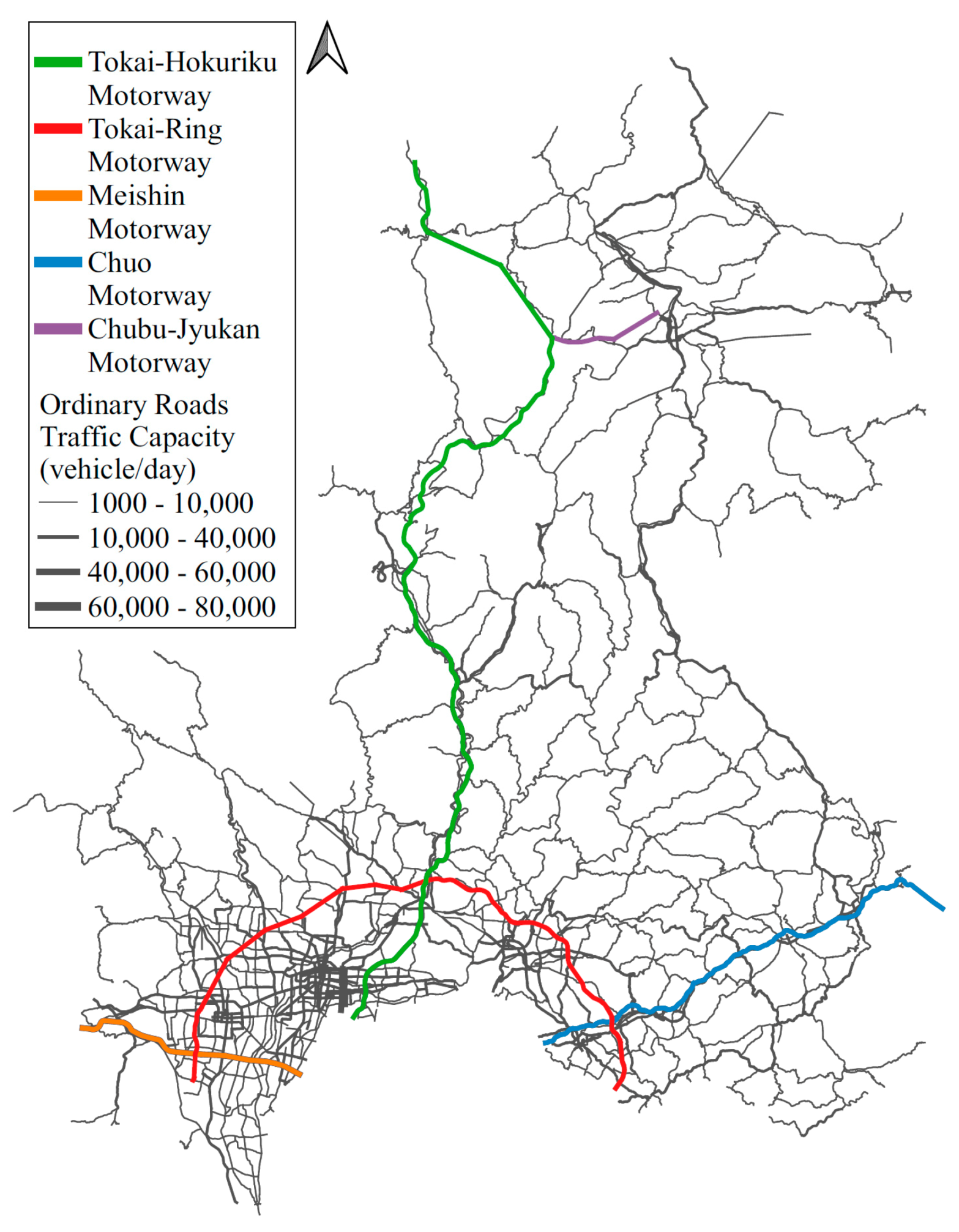
4. Target Area for Analysis and Traffic Data Used

This section introduces the history of road network improvement in the target area. Moreover, the survey data of traffic indicators used as input data are shown.

4.1. Road Improvement History in Gifu Prefecture

To understand the difference in the impact of road network improvement based on both sides of supply and demand, this study analyses the actual road network in Gifu Prefecture, Japan for a long period. Figure 1 shows the target road network. The road network includes intercity motorways, national highways and prefectural roads in both directions. Some of the motorways are under construction and are shown in their completed version. Each motorway is distinguished by line colours. Other general roads are divided into multi-step thicknesses according to their capacity. The study area is 10,620 ${\mathrm{km}}^2$ in size and includes mountainous and urban areas. Mountainous areas are more common in the north, while urban areas are more common in the south. This trend can also be seen in the density of the road network. Especially, in the southwest, there are concentrations of high-capacity roads.

In Gifu Prefecture, Japan, as is the same in other areas of Japan, based on the 14,000 km high-standard road network plan decided in 1987 by the Japanese Government, motorways have been vigorously constructed. Especially, the Tokai-Hokuriku Motorway, Tokai Ring Motorway and Chubu-Jukan Motorway have been constructed and extended. Gifu Prefecture named these three motorways as the “New three motorways” and they are regarded as effective roads for activating tourism and the economy, reducing traffic congestion and securing emergency transport roads in disasters. Figure 1 shows the locations of the “New three motorways”.

Table 2. The construction history of Tokai-Hokuriku and Tokai Ring Motorways (created by author on the basis of information on Gifu. Pref. official HP [51]).

Year	Tokai-Hokuriku Motorways	Tokai-Ring Motorways
1986	Opened Gifu-KakamigaharaIC~MinoIC L = 19.1 km (4 Lanes)
1992	Opened FukumitsuIC~Oyabe-TonamiJCT L = 11.1 km (2 Lanes)
1994	Opened MinoIC~MinamiIC L = 17.2 km (2 Lanes)
1996	Opened MinamiIC~Gujo-HachimanIC L = 10.2 km (2 Lanes)
1997	Opened Ichinomiya-KisogawaIC~Gifu-KakamigaharaIC L = 5.6 km (4 Lanes) Opened Gujo-HachimanIC~ShirotoriIC L = 16.6 km (2 Lanes)
1998	Opened BisaiIC~Ichinomiya-KisogawaIC L = 3.8 km (4 Lanes) Opened IchinomiyaJCT~BisaiIC L = 3.9 km (4 Lanes)
1999	Opened ShirotoriIC~ShokawaIC L = 21.9 km (2 Lanes)
2000	Opened GokayamaIC~FukumitsuIC L = 16.3 km (2 Lanes) Opened ShokawaIC~Hida-KiyomiIC L = 18.9 km (2 Lanes)
2002	Opened ShirakawagoIC~GokayamaIC L = 15.2 km (2 Lanes)
2004	4 Lanes completed MinoIC~Fukubegatake PA L = 18.5 km South from ShirotoriIC L = 2.1 km
2005		Opened Toyota-Higashi JCT~Mino-Seki JCT L = 73.0 km
2007	Hida tunnel opened
2008	Opened Hira-Kiyomi IC~Shirakawago IC L = 25.0 km (2 Lanes) [ALL Lanes opened] 4 Lanes completed Fukubegatake PA~Gujo-HachimanIC L = 8.9 km
2009	4 Lanes completed Gifu-YamatoIC~ShirotoriIC L = 10.4 km 4 Lanes completed Gujo-Hachiman IC~Gifu-YamatoIC L = 6.2 km	Opened Mino-Seki JCT~Seki-Hiromi IC L = 2.9 km
2012		Opened Ogaki-Nishi IC~Yoro JCT L = 5.7 km
2016		Opened ToinIC~Shin-Yokkaichi JCT L = 1.4 km
2017		Opened Yoro JCT~Yoro IC L = 3.1 km
2018	4 Lanes completed Shirotori IC~Takasu IC L = 8 km 4 Lanes completed Hirugano-Kougen SA~Hida-Kiyomi IC L = 26 km
2019	4 Lanes completed Takasu IC~Hirugano-Kogen SA L = 7 km	Opened DaianIC~ToinIC L = 6.4 km Opened Ohno-GodoIC~OgakinishiIC L = 7.6 km
2020		Opened Seki-HiromiIC~YamagataIC L = 9.0 km

summarises the construction histories and plans of the Tokai-Hokuriku Motorway and the Tokai Ring Motorway that have been actively developed. These motorways have been or will be extended to neighbouring prefectures such as Aichi, Mie, Toyama, Ishikawa and Nagano.

The Tokai Hokuriku Motorway, which was fully connected in 2008, has been continuously developed since 1996. However, some of the sections are provisionally constructed as two-lane roads, and it has been gradually expanded to four lanes. Most of the sections in Gifu Prefecture were opened in the 1990s, and the opening of the Hida Tunnel in 2007 has achieved a significant extension. On the other hand, the Tokai Ring Motorway is under construction. At first, the eastern section from Toyota East JCT to Minoseki JCT opened in 2005. After that, a construction plan was established for the western section and the construction of the western section began in 2009. The entire Tokai Ring Motorway is scheduled to open in 2026, and the total length will become about 153 km. The Tokai Ring Motorway has a lot of provisional two-lane roads, so it will be required to expand to four lanes in the future. In this way, road improvement projects have been carried out actively in Gifu Prefecture in the past few decades, and quick and effective road improvements are also required in the future.

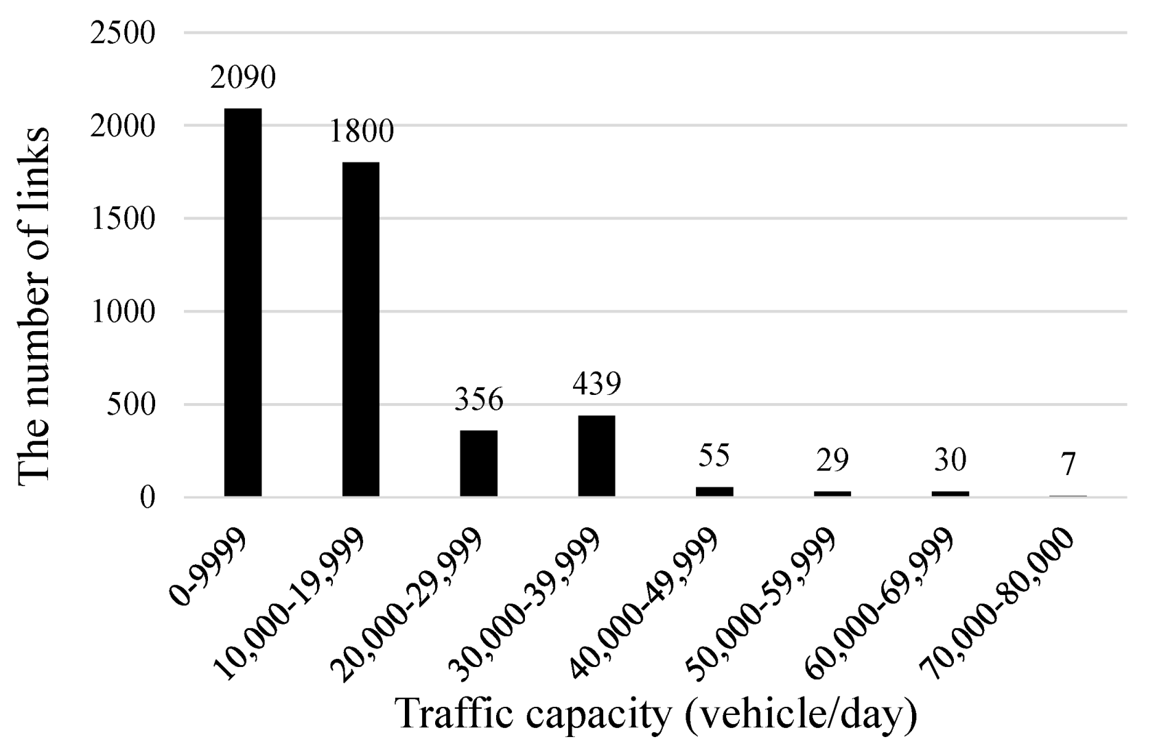
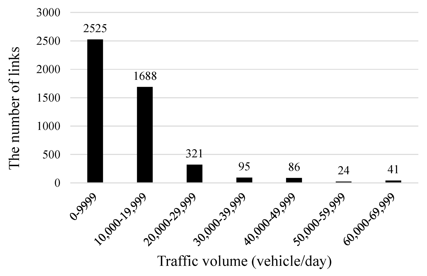
4.2. Survey Data of Roads

In Japan, a national survey is conducted periodically to understand current conditions and problems, and to correct information for future road improvement plans. This survey includes road conditions such as regulations and traffic capacity, and traffic conditions such as traffic volume, travel speed and congestion rate. In this study, the indicators of traffic capacity, length and traffic volume are used as weights to evaluate the supply and demand side. This section indicates the survey data to be used as weights.

In the history of road improvement shown in Table 2, the road networks for 4 years between 1990 and 2010 are analysed (

Table 3. Number of nodes and links in each year.

Year	1990	1999	2005	2010
Node	1727	1770	1791	1793
Link (general)	4494	4618	4717	4723
Link (motorway)	35	52	69	73

). The target road networks are in four different years: 1990, 1999, 2005 and 2010. The Gifu Prefecture road network has been improved year-on-year, as shown by the increase in nodes and links in the network (Table 3). Traffic volume, traffic capacity and length in each link used as weights are obtained from the national road traffic census survey for those years in Japan (Ministry of Land, Infrastructure, Transport and Tourism, 1990, 1999, 2005, 2010).

As an example, Figure 2, Figure 3 and Figure 4 show the distribution of the length, capacity and traffic volume in 2010. The lengths of most of the links are 5 km or less; however, there are links with a length of 15 km or more. Most of them are links representing motorways. As for traffic capacity, most of the links have capacities less than 20,000 (vehicles/day), and some of them are even smaller than 10,000. This is because a substantial number of links are narrow and are located in mountainous areas. On the contrary, there are some links with a large capacity exceeding 40,000 (vehicle/day), representing motorways. The distribution of the traffic volume is similar to that of the capacity. These distributions show that the capacity and traffic volume do not perfectly match. Although the traffic volume of most of the links is less than their capacity, some links have a traffic volume that exceeds their capacity. These are mostly located in the south of the Tokai Ring Motorway. This area has a dense road network with a concentration of links with a capacity of 10,000 (vehicles/day) or more, as can be seen from Figure 1. Most of the urban areas in Gifu Prefecture are located south of the Tokai Ring Motorway.

5. Impacts of Road Network Improvements

The eigenvector centrality (EC) of road networks in Gifu Prefecture described above is obtained by calculating the value of the eigenvector corresponding to the largest eigenvalue. The value of EC is given to the node. Nodes basically represent intersections that connect roads, but nodes are also set at places where weight values such as capacity and traffic volume change. Figure 5 shows the EC distribution for each of the four years studied. Please note that the size of the eigenvector is undermined, and the length of the eigenvector is normalised as one. The EC value is, therefore, between 0 and 1. This means that the values of EC are comparative scores in the network. Since this study focuses on the changes in the same target area, the basic topology of the road network is the same, and only newly constructed roads are additions to the networks. This paper uses MATLAB ver. R2017b to calculate the eigenvalues and the PC used was “Intel Xeon 3.50 Ghz *2, 32 GB, Windows10, 64 bit”. The road map and distribution are drawn using QGIS.

As the EC value is typically small, Figure 5 presents log-transformed values so that small differences can be more clearly distinguished. The value of node $i$ in Figure 5 is $\ln x_i^{*}$, which is always negative. Furthermore, the nodes in each network are classified into six groups according to the $\ln x_i^{*}$. Threshold values are shown in the top left part of Figure 5. The bold black roads in the network include motorways.

The area with the highest number of centrality nodes changed over time as network improvements were made. Between 1999 and 2005, it is clear that road network connectivity was improved due to the construction of the Tokai Ring Motorway (Tokai ring road), and it appears that the eastern region of Gifu became better-connected with the central area. However, there was little change in the network connectivity in 2010.

It is interesting to note that the traffic volume did not change significantly, according to the node centrality distribution, following the construction of new roads. The area with the highest-level (red) nodes in 1990 is the most urban area of Gifu Prefecture, which persists up to 2005. Then, the EC values changed substantially between 2005 and 2010. This may have been a result of the lag between road improvements and their effects, or an instantaneous effect of the substantial investment seen between 2005 and 2010. The opening of the Hida tunnel in 2008 was the largest infrastructure change in Gifu. Looking at supply and demand centrality in 2010, although the supply centrality increased in some northern regions around the Hida tunnel, the demand centrality in the northern region has not increased accordingly. This also suggests a time lag of traffic demand.

There are various backgrounds to the time lag phenomenon revealed by EC analysis. The relationship between demand and supply evaluation is verified in detail, and the causes and effects of the time lag are discussed in the next section.

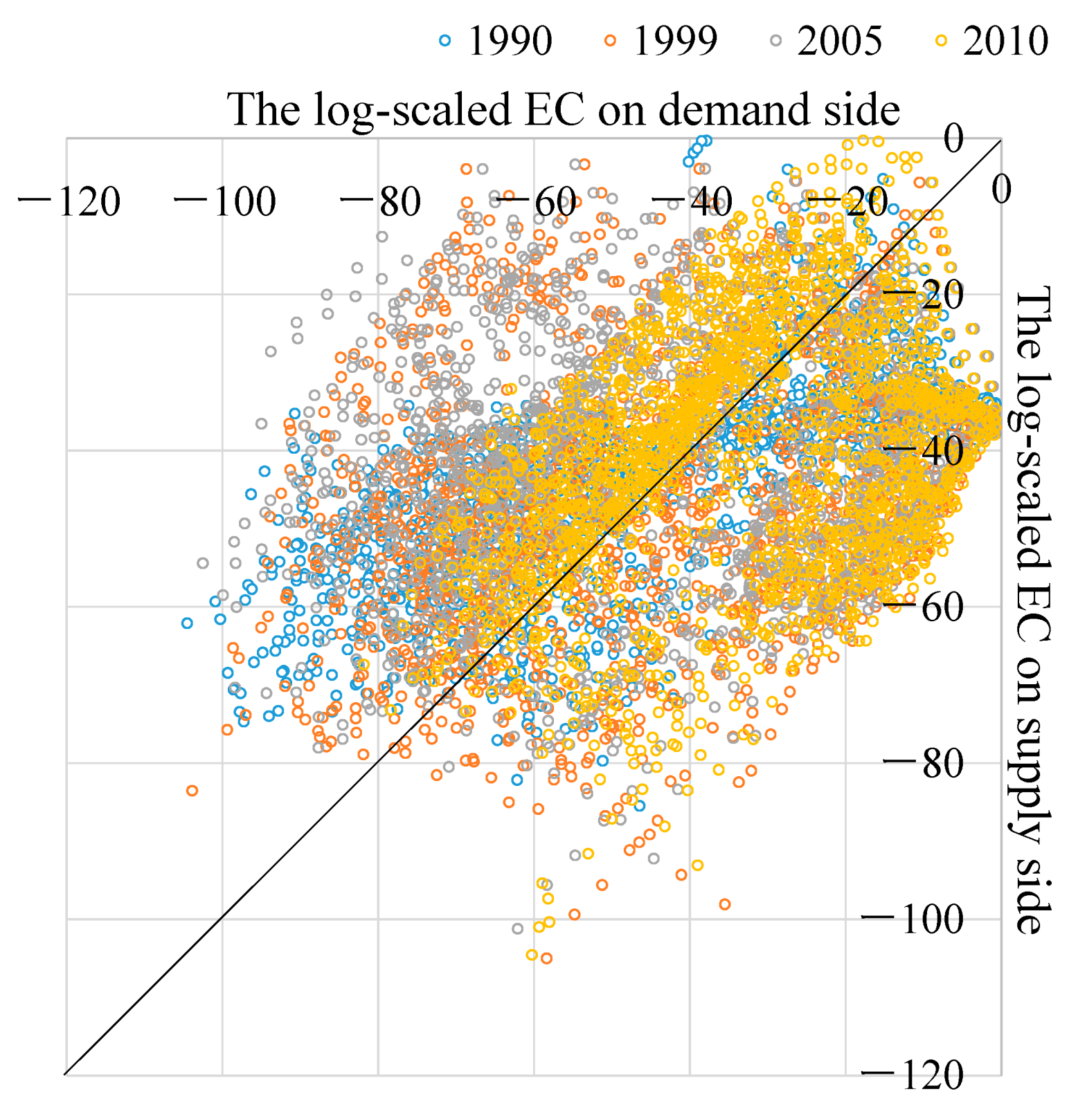
6. Relationship between Supply and Demand

The lagged effect is further investigated. The scatter plot in Figure 6 shows the difference between supply-side and demand-side evaluations at the same nodes in the same years. Plot colour represents the values in each year. For these plots, the slopes of regression lines passing through the origin of coordinates are 0.808, 0.834, 0.737 and 1.002 for years 1990, 1999, 2005 and 2010, respectively. Therefore, the nodes with high centrality evaluations on the supply side are often evaluated as low on the demand side. This means that the supply-side connectivity has been improved, but from the demand side the connectivity has not become as much as it is in the supply side. These characteristics vary from year to year.

Table 4. Correlation coefficients for supply and demand by year.

		Supply
	Year	1990	1999	2005	2010
Demand	1990	0.720	0.300	0.140	0.131
	1999	0.715	0.289	0.154	0.140
	2005	0.728	0.289	0.157	0.143
	2010	0.764	0.478	0.361	0.349

shows the correlation coefficients for supply and demand by year. Although the two types of EC values are calculated using different weights, it is interesting to note that there exist some strong correlations (up to 0.764). Here, we set two hypotheses. First, “the transport network is designed to meet the current traffic demand”, and second, “the transport demands are induced so as to meet the supply level of transport network”. If the first hypothesis is true, there should be a correlation between past demand and future supply. Thus, the correlation coefficients in Table 2 should increase when we evaluate the values from left to right. Then, if the second hypothesis is true, there should be a correlation between past supply and future demand. Thus, the correlation coefficients in Table 4 should increase when we evaluate the values from top to bottom. According to Table 4, the correlation coefficients generally increased from top to bottom, which suggests lagged effects of road investment: demand increases as supply is improved by better-connected road networks. The time required to meet with the past supply may need more than 20 years since the correlation coefficient is highest with supply in 1990 and demand in 2010.

These results may justify the significance of road improvement plans as public works. If “the transport network is designed to meet the current traffic demand”, the investment will be concentrated where the demand is already high. This may enhance traffic overconcentration. However, from the point of risk diversification and the environment, overconcentration should be avoided. Furthermore, improving connections among rural cities enhances the equity among residents. It makes sense that roads are improved to contribute to equity within the target area, and that demand responds to the supply after more than 20 years. To understand the phenomenon in more detail, the contents of these demand catch-ups should be classified into commuters, travellers and daily life. For this analysis, population data will be considered in the future.

To examine the change in EC distributions by each year, Figure 7 shows the number of nodes included in each level classified by the log-scaled EC values. From 1990 to 2005, although the number of nodes included in Level 1 is large on the demand side, there are many nodes included in Levels 4, 5 and 6. On the supply side, while the number of nodes included in Level 1 is small, the nodes included in Levels 4, 5 and 6 are also small compared with the demand side. Although it is a simple comparison of frequency distributions, Figure 7 shows that there is a difference between the demand-side distribution where the high centrality nodes increase significantly and the supply-side distribution where the low centrality nodes decrease by the road network improvements. The possible reason for this is that the connectivity of road supply performance evaluated by the supply-side EC and the concentration of traffic evaluated by the demand-side EC represent another aspect of the network. Gifu Prefecture has small cities, towns and villages throughout the network. In terms of demand, the evaluations of EC show almost no impact of such places and the nodes with lower levels may remain, so there is little “induced” demand by new road investment. On the other hand, in terms of supply, the evaluations of EC show that road network improvements have contributed to increasing connectivity to such places. The supply performance evaluated in this study is higher when the network is connected by roads with high capacity. Therefore, the effect of improvement at the highest level, such as motorways, should be very significant. The road network at higher levels is required to connect cities even if their demand is not so large. The results show that the roads in Gifu Prefecture are progressing to satisfy this requirement. As for 2010, the EC distribution drastically changes, and it resembles the supply-side distributions. As is discussed, it may be because of the lagged effect, but other factors such as depopulations, increases in tourism demand and so on should be carefully examined.

The application of changes in practical road networks for 20 years revealed that the impact of road improvements differs on the supply side and demand side. In the case of Gifu Prefecture, the evaluations on the demand side gradually increased according to the improvement in road supply performance connectivity. The correlations between the supply-side and demand-side evaluations indicate that there may be a time lag of more than a decade between them. Additionally, the change in EC distribution by each year shows the possibility of differences in the aspects of the road performance connectivity evaluated by the supply side and the concentration of traffic evaluated by the demand side.

7. Conclusions

The appearance of impact by road network improvement is greatly different depending on the side of view. In this study, we used EC to evaluate the actual road network in terms of supply and demand. Firstly, the supply- and demand-weighted EC values were used to evaluate the impact of road network improvements. The history of actual road improvement was summarised, and the road network as of each year point was evaluated based on supply and demand sides. The changes in EC values seen in each of the four years analysed point to differences in road service connectivity and traffic concentrations. The results showed that the road improvements affected supply and demand separately over the 20-year study period.

Furthermore, analysis of the relationship between these results over time provided some interesting knowledge. In Gifu Prefecture, demand increased gradually in response to the improved road service connectivity. It was concluded that the impact of road improvement on the demand side may have a lagged effect. Focusing on areas where the road network actually changes significantly, we have shown that there is a time lag in changes related to improved connectivity and traffic concentration. Such analyses are useful for understanding the impact of road improvements across an entire network, not only local change. Since analysis can be performed using only the indicators as the characteristic values and the data of graph structure, an extensive area and long-term evaluation is possible. Road construction is a long-term project; therefore, this method is useful for verifying when and how the effects of road improvements will be shown in each aspect such as user, administrator and disaster prevention.

The following is a list of future tasks. The first point is the range of the target area. The target network in this study was limited to Gifu Prefecture. However, the improvement of the roads discussed has a significant effect on increasing accessibility to other prefectures. There may be improvements that can produce more effective results when the target area is extended to the surrounding prefectures. It is necessary to consider the road network outside Gifu Prefecture to verify such effects. Another point is the addition of other elements. This paper adopted the connectivity of road networks as the supply side and the concentration of traffic as the demand side. However, there are many other factors that constitute supply and demand. For example, the supply-side changes are rail networks, housing and workplace information, and also the demand-side changes are OD pattern and population. Each of these will have a specific impact and speed of change. These characteristics need to be evaluated comprehensively. These factors will be analysed for differences based on the method for evaluating long-term relationships shown in this study.

References

1. Research Report: Study on Personal Passenger Car Traffic Regulation Following the Great Earthquake Disaster. Int. Assoc. Traffic Saf. Sci. 2002, 23, 3. (In Japanese)
2. Cutini, V.; Pezzica, C. Street network resilience put to the test: The dynamic crash of Genoa and Bologna bridges. Sustainability 2020, 12, 4706. [Google Scholar] [CrossRef]
3. Wegener, M. Operational urban models state of the art. J. Am. Plan. Assoc. 1994, 60, 17–29. [Google Scholar] [CrossRef]
4. Iacono, M.; David, L.; Ahmed, E.G. Models of transportation and land use change: A guide to the territory. J. Plan. Lit. 2008, 22, 323–340. [Google Scholar] [CrossRef]
5. Forrester, J.W. Urban dynamics. IMR Ind. Manag. Rev. 1970, 11, 67. [Google Scholar] [CrossRef] [Green Version]
6. Wegener, M. Overview of land use transport models. In Handbook of Transport Geography and Spatial Systems; Emerald Group Publishing Limited: Bingley, UK, 2004; Volume 9, pp. 127–146. [Google Scholar]
7. Hunt, J.D.; Kriger, D.S.; Miller, E.J. Current operational urban land use–transport modelling frameworks a review. Transp. Rev. 2005, 25, 329–376. [Google Scholar] [CrossRef]
8. Kii, M.; Nakanishi, H.; Nakamura, K.; Doi, K. Transportation and spatial development: An overview and a future direction. Transp. Policy 2016, 49, 148–158. [Google Scholar] [CrossRef]
9. Alonso, W. Location and Land Use; Harvard University Press: Cambridge, UK, 1964. [Google Scholar]
10. Herbert, J.D.; Stevens, B.H. A Model for the distribution of residential activity in urban areas. J. Reg. Sci. 1960, 2, 21–36. [Google Scholar] [CrossRef]
11. Fujita, M. Urban Economic Theory; Cambridge University Press: Cambridge, UK, 1989. [Google Scholar]
12. Anas, A. Residential Location Markets and Urban Transportation, Economic Theory, Econometrics and Policy Analysis with Discrete Choice Models; Academic Press Inc.: London, UK, 1982. [Google Scholar]
13. Lowry, I.S. A Model of Metropolis; Rand Corp: Santa Monica, CA, USA, 1964. [Google Scholar]
14. Anas, A.; Arnott, R.; Small, K.A. Urban spatial structure. J. Econ. Lit. 1998, 36, 1426–1464. [Google Scholar]
15. Salvani, P.; Miller, E.J. ILUTE: An operational prototype of a comprehensive microsimulation model of urban systems. Netw. Spat. Econ. 2005, 5, 217–234. [Google Scholar] [CrossRef]
16. Musolino, G. Modelling long-term impacts of the transport supply system on land use travel demand in urban areas. Eur. Transp. 2008, 40, 69–87. [Google Scholar]
17. Wegener, M. Integrated land-use transport modelling progress around the globe. In Proceedings of the Fourth Oregon Symposium on Integrated Land-Use Transport Models, Portland, OR, USA, 13–16 July 2005; pp. 15–17. [Google Scholar]
18. Patarasuk, R.; Binford, M.W. Longitudinal analysis of the road network development and land-cover change in Lop Buri province, Thailand, 1989–2006. Appl. Geogr. 2012, 32, 228–239. [Google Scholar] [CrossRef]
19. Santos, B.; Antunes, A.; Miiler, E.J. Integrating equity objectives in a road network design model. Transp. Res. Rec. 2008, 2089, 35–42. [Google Scholar] [CrossRef] [Green Version]
20. Garrison, W.L. Connectivity of the interstate highway system. Reg. Sci. Assoc. Pap. Proc. 1960, 6, 121–137. [Google Scholar] [CrossRef]
21. Garrison, W.L.; Marble, D.F. The Structure of Transportation Networks; Technical Report 62; U.S. Army Transportation Command: Scott Air Force Base, IL, USA, 1962; pp. 73–88. [Google Scholar]
22. Kansky, K. Structure of Transportation Networks: Relationships between Network Geometry and Regional Characteristics. Doctoral Dissertation, Department of Geography, University of Chicago, Chicago, IL, USA, 1963. [Google Scholar]
23. Haggett, P.; Chorley, R.J. Network Analysis in Geography; Edward Arnold: London, UK, 1969; p. 56. [Google Scholar]
24. Medvedkov, Y.V. An application of topology in central place analysis. Pap. Proc. Reg. Sci. 1968, 20, 77–84. [Google Scholar] [CrossRef]
25. Royaltey, H.H.; Astrachan, E.; Sokal, R.R. Tests for patterns in geographic variation. Geogr. Anal. 1975, 7, 369–395. [Google Scholar] [CrossRef]
26. Xie, F.; Levinson, D. Measuring the structure of road networks. Geogr. Anal. 2007, 39, 336–356. [Google Scholar] [CrossRef]
27. Latora, V.; Marchiori, M. Efficient behavior of small-world networks. Phys. Rev. Lett. 2001, 87, 198701. [Google Scholar] [CrossRef] [Green Version]
28. Bavelas, A. A mathematical model for group structures. Appl. Anthropol. 1949, 7, 16–30. [Google Scholar] [CrossRef]
29. Newman, M.E.J. Networks; Oxford University Press: Oxford, UK, 2010. [Google Scholar]
30. Morgado, P.; Costa, N. Graph-based model to transport networks analysis through GIS. In Proceedings of the European Colloquium on Quantitative and Theoretical Geography, Athens, Greece, 2–5 September 2011. [Google Scholar]
31. Erath, A.; Lochl, M.; Axhausen, K.W. Graph-theoretical analysis of the swiss road and railway networks over time. Netw. Spat. Econ. 2009, 9, 379–400. [Google Scholar] [CrossRef] [Green Version]
32. Casali, Y.; Heinimann, H.R. A topological analysis of growth in the Zurich road network. Comput. Environ. Urban Syst. 2019, 75, 244–253. [Google Scholar] [CrossRef]
33. Lämmer, S.; Gehlsen, B.; Helbing, D. Scaling Laws in the Spatial Structure of Urban Road Networks. Phys. A Stat. Mech. Its Appl. 2006, 363, 89–95. [Google Scholar] [CrossRef] [Green Version]
34. Duan, Y.; Lu, F. Robustness of city road networks at different granularities. Phys. A Stat. Mech. Its Appl. 2004, 411, 21–34. [Google Scholar] [CrossRef]
35. Jiang, B.; Claramunt, C. A Structural Approach to the Model Generalization of an Urban Street Network. Geoinformatica 2004, 8, 157–171. [Google Scholar] [CrossRef]
36. Crucitti, P.; Latora, V.; Porta, S. Centrality in networks of urban streets. Phys. Rev. E 2006, 73, 036125. [Google Scholar] [CrossRef] [PubMed] [Green Version]
37. Porta, S.; Crucitti, P.; Latora, V. Multiple centrality assessment in Parma: A network analysis of paths and open spaces. Urban Des. Int. 2008, 13, 41–50. [Google Scholar] [CrossRef] [Green Version]
38. Proctor, C.H.; Loomis, C.P. Analysis of sociometric data. In Research Methods in Social Relations; Holland, P.W., Leinhardt, S., Eds.; Dryden Press: New York, NY, USA, 1951; pp. 561–586. [Google Scholar]
39. Bonacich, P. Factoring and weighting approaches to status scores and clique identification. J. Math. Sociol. 1972, 2, 113–120. [Google Scholar] [CrossRef]
40. Beauchamp, M.A. An improved index of centrality. Behav. Sci. 1965, 10, 161–163. [Google Scholar] [CrossRef]
41. Freeman, L. A set of measures of centrality based on betweenness. Sociometry 1977, 40, 35–41. [Google Scholar] [CrossRef]
42. Katz, L. A New Status Index Derived from Sociometric Analysis. Psychometrika 1953, 18, 39–43. [Google Scholar] [CrossRef]
43. Brin, S.; Page, L. The anatomy of a Large-Scale hypertextual web search engine. In Proceedings of the Seventh International World-Wide Web Conference, Brisbane, Australia, 12–18 April 1998; pp. 107–117. [Google Scholar]
44. Martin, T.; Zhang, X.; Newman, M.E. Localization and centrality in networks. Phys. Rev. E 2014, 90, 052808. [Google Scholar] [CrossRef] [Green Version]
45. Barabasi, A.; Bonabeau, E. Scale-Free networks. Sci. Am. 2003, 288, 50–59. [Google Scholar] [CrossRef]
46. Bihari, A.; Pandia, M.K. Key author analysis in research professionals’ relationship network using citation indices and centrality. Procedia Comput. Sci. 2015, 57, 606–613. [Google Scholar] [CrossRef] [Green Version]
47. Borgatti, S.P. Centrality and network flow. Soc. Netw. 2005, 27, 55–71. [Google Scholar] [CrossRef]
48. Landherr, A.; Friedl, B.; Heidemann, J. A critical review of centrality measures in social networks. Busines Inf. Syst. Eng. 2019, 2, 371–385. [Google Scholar] [CrossRef]
49. Ando, H.; Bell, M.; Kurauchi, F.; Wong, K.I.; Cheung, K.F. Connectivity evaluation of large road network by capacity-weighted eigenvector centrality analysis. Transp. A Transp. Sci. 2021, 17, 648–674. [Google Scholar] [CrossRef]
50. Cheung, K.F.; Bell, M.G.; Pan, J.J.; Perera, S. An eigenvector centrality analysis of world container shipping network connectivityk. Transp. Res. Part E 2020, 140, 101991. [Google Scholar] [CrossRef]
51. Gifu Prefecture. Japan Official Homepage. Available online: https://www.pref.gifu.lg.jp/site/english/ (accessed on 15 October 2021).
Figure 1. Road networks in Gifu Prefecture and the location of motorways.
Sustainability 13 13366 g001
Figure 2. The distribution of length in 2010.
Sustainability 13 13366 g002
Figure 3. The distribution of capacity in 2010.
Sustainability 13 13366 g003
Figure 4. The distribution of traffic volume in 2010.
Sustainability 13 13366 g004
Figure 5. The long-term distribution of eigenvector centrality (EC) values according to the supply–demand weights. (a) Supple side (Capacity and Length) in 1990; (b) Demand side (Traffic Volume) in 1990; (c) Supple side (Capacity and Length) in 1999; (d) Demand side (Traffic Volume) in 1999; (e) Supple side (Capacity and Length) in 2005; (f) Demand side (Traffic Volume) in 2005; (g) Supple side (Capacity and Length) in 2010; (h) Demand side (Traffic Volume) in 2010.
Sustainability 13 13366 g005aSustainability 13 13366 g005b
Figure 6. Scatter plot in EC on both weights.
Sustainability 13 13366 g006
Figure 7. The number of nodes in each level.
Sustainability 13 13366 g007