Detailed Analysis of Spatial–Temporal Variability of Rainfall Erosivity and Erosivity Density in the Central and Southern Pannonian Basin

Abstract

Estimation of rainfall erosivity (RE) and erosivity density (ED) is essential for understanding the complex relationships between hydrological and soil erosion processes. The main objective of this study is to assess the spatial–temporal trends and variability of the RE and ED in the central and southern Pannonian Basin by using station observations and gridded datasets. To assess RE and ED, precipitation data for 14 meteorological stations, 225 grid points. and an erosion model consisting of daily, monthly, seasonal, and annual rainfall for the period of 1961–2014 were used. Annual RE and ED based on station data match spatially variable patterns of precipitation, with higher values in the southwest (2100 MJ·mm·ha⁻¹·h⁻¹) and southeast (1650 MJ·mm·ha⁻¹·h⁻¹) of the study area, but minimal values in the northern part (700 MJ·mm·ha⁻¹·h⁻¹). On the other hand, gridded datasets display more detailed RE and ED spatial–temporal variability, with the values ranging from 250 to 2800 MJ·mm·ha⁻¹·h⁻¹. The identified trends are showing increasing values of RE (ranging between 0.20 and 21.17 MJ·mm·ha⁻¹·h⁻¹) and ED (ranging between 0.01 and 0.03 MJ·ha⁻¹·h⁻¹) at the annual level. This tendency is also observed for autumn RE (from 5.55 to 0.37 MJ·mm·ha⁻¹·h⁻¹) and ED (from 0.05 to 0.01 MJ·ha⁻¹·h⁻¹), as for spring RE (from 1.00 to 0.01 MJ·mm·ha⁻¹·h⁻¹) and ED (from 0.04 to 0.01 MJ·ha⁻¹·h⁻¹), due to the influence of the large-scale processes of climate variability, with North Atlantic Oscillation (NAO) being the most prominent. These increases may cause a transition to a higher erosive class in the future, thus raising concerns about this type of hydro-meteorological hazard in this part of the Pannonian Basin. The present analysis identifies seasons and places of greatest erosion risk, which is the starting point for implementing suitable mitigation measures at local to regional scales.

1. Introduction

Climate change is considered to have the most challenging worldwide environmental impact and soil erosion is expected to vary in response to changes in climate variables [1]. As highlighted by Azari et al. [2], it has several important implications for soil resources that are reflected in overall variations in the rainfall amount, intensity, spatial–temporal distribution, and increment in extreme precipitation events. The most direct effects of climate change on soil erosion are changes in rainfall erosivity due to changes in rainfall intensity [3] and the occurrence of extreme precipitation [4,5,6].

Water erosion is one of the most prominent causes of land degradation [7,8]. As highlighted by Grillakis et al. [9], the interplay between soil and rainfall has an important role regarding the ecological, hydrological, and biogeochemical cycles, since rainfall-induced soil erosion significantly affects its functions, and alters the soil structure and organic matter content. Therefore, soil erosion can be perceived as a widespread ecological and environmental crisis that poses a serious threat to the future quality of human life [10]. Xu et al. [11] highlight that this type of hydro-meteorological hazard is highly related to many natural factors, including rainfall (amount and variability), topography, soil, and vegetation properties, as well as human activities that intensify erosion processes. Water erosion has many on- and off-site effects [12], but off-site effects may have greater social, economic, and environmental impacts [13]. Soil erosion impacts deleteriously on land resources and develops flood-related risks. It also affects water quality degradation through the transportation of pesticides, fertilisers, and nutrients by the sediment [8]. The Pannonian Basin is known as a major agricultural region in Europe [14], so the impact of soil erosion and land degradation may severely affect regional agricultural production and the national economy of the states in this region. Therefore, more attention should be oriented towards soil erosion caused by rainfall in this area.

Since numerous studies around the world have shown that rainfall is the main climatological factor leading to soil erosion, with raindrop splash erosion and runoff being the main characteristics that influence this process, contemporary studies have focused on observing parameters described as rainfall erosivity—RE, e.g., [15,16,17,18,19,20,21,22,23,24,25,26]. Certain authors recognise this parameter as the potential of raindrops to trigger soil erosion, where its estimation is fundamental for the understanding of the climatic vulnerability within a given region, e.g., [11,27]. This geomorphic process can be illustrated in Figure 1.

In the previous conceptual framework, a quantitative assessment of potential soil erosion caused by rainfall is used for predicting soil erosion and for improving soil and water conservation and management. According to Bezak et al. [26], RE is an index that quantitatively describes the rainfall-driven force for soil erosion and is often regarded as one of the most important factors affecting the spatial and temporal variability of various soil erosion displacement processes. RE is expressed as the product of the total kinetic energy of a rainfall event times the 30-min maximum rainfall intensity [28]. It is calculated using high-resolution pluviographic data from rain gauges [10,11,17,29,30,31] or by simpler models based on daily, monthly, seasonal, and annual rainfall [10,11,17,23,24,25,26,27,28,29,30]. RE is one of the key input parameters of the universal soil loss equation (USLE) and the revised universal soil loss equation (RUSLE) [11,19,21,26,32]. Additionally, erosivity density (ED) is observed as the proportion of RE to precipitation [11].

Climate change is expected to affect future rainfall attributes due to a rise in the humidity in the atmosphere during a warmer climate [33]. The Intergovernmental Panel on Climate Change (IPCC) document “Special Report on Climate Change and Land”, presents evidence of how these changes substantially affect other processes. These processes encompass desertification (water scarcity), land degradation (soil erosion, vegetation loss, wildfire, permafrost thaw), and food security (crop yield and food supply uncertainty) [23,34]. Moreover, an increase in severe storm intensity will likely enhance runoff and decrease the soil water infiltration process, thus causing even greater soil losses than at the beginning of the 21st century [19,20,23,24,25,30]. Soil erosion already accounts for most soil loss, compared to other erosion processes in Europe, even though RE had only increased by 4% during the last decades of the 20th century [23,25].

Numerous respective researchers worldwide discussed the spatial–temporal variability of rainfall erosivity in study regions: from world study conducted by Borelli et al. [35] to Australia [36,37] and New Zeland [38], Africa [39,40,41], Brasil [42,43], Columbia [44], China [10,11,17,30,45], South Korea [45,46], Iran [2,47], and Uzbekistan [48]. Small-scale studies in the Pannonian Basin [8], Tuscany [49], Rhone region [50], Greece [21], Czech Republic [51], and the Netherlands [52] also suggest a positive trend in RE during the last 50 years. What all the studies have in common is that rainfall erosivity poses a significant environmental threat that needs to be thoroughly addressed.

Since the Pannonian Basin is an intensive agriculture area, the present study extends previous research in the Basin [8] to gain a better insight into soil loss in the light of precipitation variability. Despite limited data in the Western Balkans, this research strives to fill a gap in information for the central and southern parts of the Pannonian Basin in Southeast Europe (northern Serbia-Vojvodina, Hungary, and the eastern part of Croatia).

The main objectives of this study are: (1) to investigate spatial–temporal trends and variability of the RE and ED in the central and southern Pannonian Basin by using different data repositories (ECA&D and E-OBS), and (2) to emphasise the importance of the influence of the large-scale processes of climate variability. Particular attention is placed on multi-decadal trends and variability in these two indices. The findings will add to European erosivity studies by filling in gaps in the erosivity map provided by Panagos et al. [19,20], plus they will improve understanding of RE and ED variability at local to regional scales. This study will also provide useful reference information for soil erosion risk assessment and soil conservation planning in the Pannonian Basin since it comprises a large percentage of arable land (Figure 1).

2. Materials and Methods

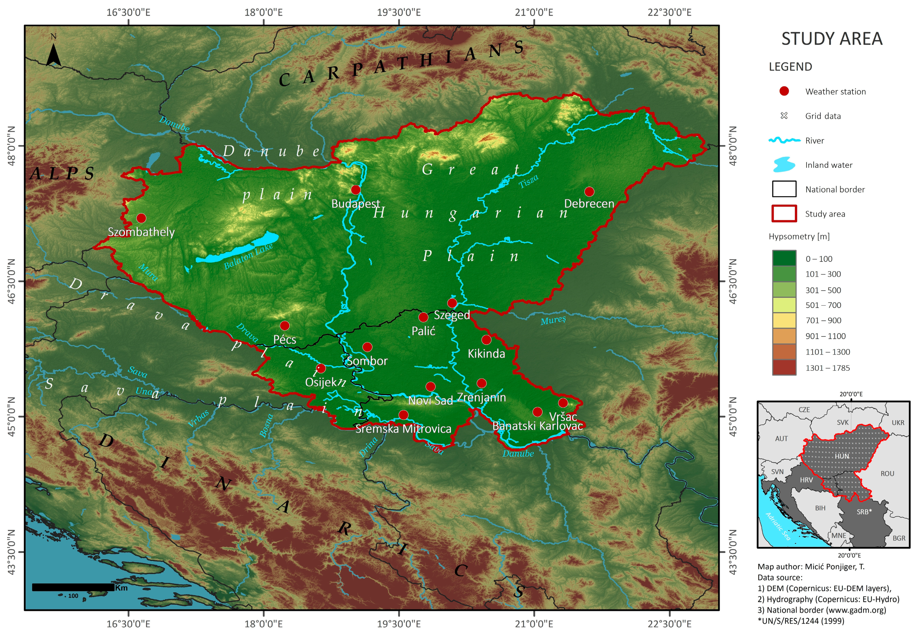
2.1. Study Area

The Pannonian Basin (referring to modern-time state boundaries) in central Europe, extends over the Czech Republic, Austria, Slovenia, Hungary, Croatia, Bosnia and Herzegovina, Serbia, Romania, Slovakia, and Ukraine [53]. The Carpathians in the north and east, the Dinaric in the south, and the Alps in the west surround this region [54]. Additionally, four pivotal plains of the region, such as the Great Hungarian Plain, the Danube plain, the Sava plain, and the Drava plain, highlight its orographic characteristics [55]. This study area covered in this research encompasses the territories of Hungary, northern Serbia (A.P. Vojvodina), and the eastern part of Croatia (Osijek-Baranja County), with the topographic range from 80 m above sea level (m.a.s.l.) to 203 m.a.s.l. (Figure 2).

Since the Pannonian Basin is located in the Northern Hemisphere mid-latitudes, the lowest air temperature values occur in January and the highest in July and August. The average annual air temperature fluctuates between 9.7 °C in Hungary to 11 °C in Vojvodina and 12.5 °C in eastern Croatia. The rainfall season ranges from mid-April to September, and cloud cover is highest from November to January. The average amount of precipitation is approximately 600 mm per year [8]. Wind speed was found to decrease in every season throughout the year, while relative humidity is increased in autumn and decreased in spring, summer, and winter during the period of 1960–2010 [54]. On the other hand, sunshine duration has the opposite trend [8].

The investigated area has a high diversity of physical, biophysical, and socioeconomic conditions. During the past few decades, an increasing number of extreme hydrometeorological events (heat waves, droughts, heavy precipitation, etc.) have been reported [8,56,57,58,59,60,61], favouring increased rainfall erosivity for most of the investigated area, except in the northwestern parts. Using four pluvial indices, Lukić et al. [8] showed that precipitation extremes have been rising in terms of totals and intensities. Climate change projections suggest that there will be consequences within multiple sectors of the observed Pannonian Basin, counting as well the lethal impacts on its ecosystem services. Being that this part of Europe represents one of the regional hotspots, it is crucial to say that it is regarded as the region with the highest number of severely affected sectors in the whole of Europe [62].

2.2. Data

Daily rainfall data from meteorological stations were obtained from the European Climate Assessment and Dataset (ECA&D) to estimate RE and ED for the period of 1961–2014. In this data repository, daily precipitation values (RR) are calculated as the sum of RR of 18 UT of the current day and RR of 06 UT of the next day. The snow was not included in RR since the indices used in the study do not require this parameter. Only validated RR values were used, indicated by the flag 0 in the column labelled quality control (QC) from the ECA&D data repository [63]. Daily ECA&D RR series at each site were tested and homogenised by Wijngaard et al. [64].

As pointed out by Thornton et al. [65], gridded weather products are generally used to support ecological, agricultural, water resources management, and climate change studies, more particularly in regions with sparse meteorological stations. Being that gridded data exhibit a high resolution on spatial and temporal distributions of weather products, the European Observations (E-OBS) datasets were used in this study. The latest version v23.1e, in regular latitude–longitude coordinates and regular horizontal resolution of 0.25° × 0.25° were used as well. The produced database, given as part of the EU ENSEMBLES project, is comprised of daily mean, minimum, and maximum temperature values and daily precipitation, respectively. Total daily amounts of precipitation (RR) in mm (measured as the height of the equivalent liquid water in a square meter) are included within the observed datasets. The data sources for the precipitation are rain gauge data which do not possess a uniform way of defining the 24 h, after which the precipitation measurements were made. Therefore, there is no uniform time for the measurement period, which could be attributed to the daily precipitation. The Global 30 Arc-Second Elevation Dataset (GTOPO30) is used for the elevation file. It represents a global raster digital elevation model (DEM) with a horizontal grid spacing of 30 arc seconds (approximately 1 kilometre) that is developed by USGS [63,66]. The above-described dataset is comprised of 225 grids and was used to produce a high spatial resolution of RE and ED maps on multiannual and seasonal scales.

The monthly, seasonal, and annual series were derived from daily series. Standard season definitions are used, namely: winter (DJF), spring (MAM), summer (JJA), and autumn (SON). A list of the meteorological stations used in the study is given in

Table 1. Meteorological stations were used in this study for the period of 1961–2014. Country codes are Serbia (SRB), Hungary (HUN), and Croatia (HRV).

No.	Station Name	Country	Latitude (N)	Longitude (E)	Altitude (m)
1.	Sombor	SRB	45°46′12″	19°09′00″	87
2.	Palić	SRB	46°06′00″	19°46′12″	102
3.	RimskiŠančevi	SRB	45°19′48″	19°51′00″	86
4.	Kikinda	SRB	45°51′00″	20°28′12″	81
5.	Zrenjanin	SRB	45°22′00″	20°25′00″	80
6.	Banatski Karlovac	SRB	45°03′00″	21°02′12″	100
7.	Vršac	SRB	45°09′00″	21°19′12″	83
8.	Sremska Mitrovica	SRB	45°01′00″	19°33′00″	82
9.	Pécs	HUN	46°00′21″	18°13′58″	203
10.	Szeged	HUN	46°15′22″	20°05′25″	82
11.	Debrecen	HUN	47°29′25″	21°36′39″	108
12.	Budapest	HUN	47°30′40″	19°01′14″	153
13.	Szombathely	HUN	47°11′54″	16°38′52″	201
14.	Osijek	HRV	45°32′00″	18°38′00″	88

.

2.3. Methodology

All steps, including procedures and different quantitative approaches used in this research, are presented in the following workflow (Figure 3).

Numerous indices have been used to quantify water erosion, among which the most prominent are Fourier index (FI) and modified Fourier index (MFI). These indices are based on monthly rainfall data averages since high-quality datasets on a regional scale are very scarce [8,55]. R factor reflects the potential capability of precipitation to cause soil loss and is one of the most important factors for estimating soil erosion. In its humblest formula, the R factor stands for an average annual value and is quantified by summing the event-based energy-intensity values (EI₃₀) for a specific site divided by the number of observed years [10,11]. The relationship between FI and MFI with the USLE R has been discussed [8,55]. The main difference between the previously mentioned indices and the one used here is in the erosional rate estimation that is best represented by RE and ED [10,11,17,67].

The value of RE was calculated following Zhang et al. [68]:

$$R{E}_i=\alpha {\displaystyle \sum }_{j=1}^k{\left(P_j\right)}^{\beta }$$

(1)

where RE_i is the rainfall erosivity in i-th half-month (MJ·mm·ha⁻¹·h⁻¹). Each month was separated into two half-months: from 1st–15th and from 16th to the end of the month; dividing a year into 24 half-months. P_j represents the erosive rainfall on the j-th day (mm) when actual rainfall was >12 mm. If the actual daily rainfall was <12 mm, then the P_j was counted as zero. Parameter k represents the number of days in the i-th half-month [68].

The values of α and β, as empirical parameters, were determined as follows:

$$\beta =0.8363+\frac{18.177}{{\overline{P}}_{d12}}+\frac{24.455}{{\overline{P}}_{y12}}$$

(2)

$$\alpha =21.586{\beta }^{-7.1891}$$

(3)

where $\overline{P}$_d12 and $\overline{P}$_y12 present the average daily/annual erosive rainfall when daily rainfall is >12 mm.

ED is the ratio of rainfall erosivity to precipitation [67]. It measures the erosivity per rainfall (in mm) and is expressed as MJ·ha⁻¹·h⁻¹. The equation can be applied on a monthly or yearly scale (i).

$$E{D}_i=\frac{R{E}_i}{P_i}$$

(4)

The direct measurement of kinetic energy (KE) requires sophisticated and costly instruments. Methods utilized for the estimation of KE, based on power functions, are proven to be valid in practice. Due to the limited availability of hyetograph and disdrometer data, statistical models that use available data on daily precipitation were created. Three main aspects of the R factor are considered when performing soil erosion estimations. One is the average annual rainfall erosivity for the prediction of average annual soil loss. The second one is based on the seasonal distribution values of rainfall erosivity, and the third one represents the event or daily rainfall erosivity, which is crucial for the analysis of the soil loss recurrence and its assessment. Models that use events or daily rainfall as measurements for the calculation of erosivity, exhibited at all temporal scales, are significant. Moreover, those can satisfy the three usage requirements mentioned previously in the context. A power-law function has been generally used for the estimation of erosion index EI₃₀ gathered from the event or daily rainfall amounts. A connection between EI₃₀ index, obtained for the half-month period, and the sum of the estimated daily erosivity for the same period, has been tested by Xie et al. [69]. This approach was considered the average annual rainfall erosivity and its seasonal variations, while attention was not particularly given to the estimations of daily rainfall erosivity. It is crucial to say that this approach is suitable for the analysis of seasonal differences in rainfall characteristics. As highlighted by Teng et al. [70], a power function model observed by Zhang et al. [68] showed that the estimated R factor, used in this model, aligns well with the EI₃₀ index (R² = 0.72). Zhang et al. [68] also reported a strong correlation between the parameters α and β (R² = 0.95). Additionally, analysis of the maximum daily precipitation data indicates that a defined 12.0 mm threshold (used for a daily rainfall amount model) is similar to the threshold of 12.7 mm, as suggested by Wishmeier and Smith [71]. Therefore, this proposal can be used as a practical threshold for the separation of erosive and non–erosive storms within a given area [72]. Since (1) empirical parameters α and β are closely related to climate characteristics and topography of the study area, and (2) the presence of good agreement between R factor and EI₃₀ due to high-resolution data scarcity, the authors decided to apply Zhang’s power-law function model for the estimation of RE and ED.

Trends in time series of RE and ED were analysed via the nonparametric Mann–Kendall (M–K) test. The M–K test is widely used because it does not require a normal distribution of data and is straightforward to calculate [17]. Two hypotheses are set here: the null hypothesis (H₀), which states that there is no trend in the time series; the alternative hypothesis (H_a), which states that there is a significant trend in the series, for a given level of significance. Here, the trend is regarded as statistically significant at the following confidence levels (p): 0.1, 0.05, and 0.01, respectively. If the p-value is lower than the specified level, H₀ should be rejected, accepting H_a and vice versa. To prevent the effects of the serial correlation in observed time series, the Yue–Pilon method was applied [73].

To examine the relationship between the number of heavy precipitation days (R10mm) and potential climate driver North Atlantic Oscillation (NAO), Pearson correlation (r) with 0.01 and 0.05 confidence levels was utilized following the approach of Lukić et al. [8]. To examine the relationship between extreme precipitation index (R10mm) and NAO, linear correlations (the Pearson correlation coefficient) were utilised. Within this methodological approach, a correlation of +1 or −1 occurs when each of the variables is perfectly correlated to the other. On the other hand, a correlation close to zero means that there is a weak relationship between the examined variables. The values of NAO were obtained from the Climatic Research Unit of the University of East Anglia following the approach of Jones et al. [74].

The spatial distribution of RE and ED was produced using the radial basis function interpolation method with the inverse multiquadric (RBF IMQ) kernel. This technique tends to estimate the wide rainy areas and smooth rainfall fields using a small number of observed data to obtain higher accuracy. Contrary to the conventional inverse distance weighting (IDW) interpolation method or RBF with inverse quadratic (IQ) kernel, which tends to approximate the wide rainy areas and smooth rainfall field when using a small number of observations, the RBF IMQ does not flatten the field, even when the same smoothing parameter is used as in the usual RBF and IDW [75]. The same method for visualisation of the results was used in previous studies regarding rainfall erosivity (e.g., Lukić et al. 2018 [52], and Lukić et al. 2019 [8]).

3. Results

3.1. Intra-Annual Distribution of RE and ED

The annual distribution of RE for the central and southern Pannonian Basin was binned and plotted by decade to better highlight temporal variability in RE (Figure 4a). The boxen plots for RE (seaborn module, boxen plot) are conducted for gridded data, due to the data volume (225 grids). As boxen plots are showing minimum, maximum, and median in the dataset boxes, and plot more quantiles, they provide a better insight into the shape of the distribution, particularly in the tails (Figure 4d–f). Overall, maximum mean long-term RE values were recorded for stations Pécs (2100 MJ·mm·ha⁻¹·h⁻¹) and Osijek (2093 MJ·mm·ha⁻¹·h⁻¹). Interestingly, the maximum value for the last decade occurred in Vršac (3739 MJ·mm·ha⁻¹·h⁻¹), which had a similar RE distribution to other stations until the most recent decade. Minimal average value through the decades (Figure 4a), as well as variation in RE, is recorded for Budapest meteorological station (703 MJ·mm·ha⁻¹·h⁻¹).

Paying attention to the median on the boxen plot (Figure 4d), we can highlight that RE values are slightly rising since the 1980s, with their maximum detected in the last decade. This finding is consistent with station data, as well as with the previous studies [8,55,76,77,78,79,80].

The seasonal variability of RE is pronounced. Summer has the highest mean RE values (709 MJ·mm·ha⁻¹·h⁻¹), followed by the means for autumn (351 MJ·mm·ha⁻¹·h⁻¹), spring (314 MJ·mm·ha⁻¹·h⁻¹), and winter (139 MJ·mm·ha⁻¹·h⁻¹) (Figure 4b). Szombathely is the station with the highest summer RE (975 MJ·mm·ha⁻¹·h⁻¹), and Budapest the lowest (260 MJ mm·ha⁻¹·h⁻¹). Only three meteorological stations have autumn mean RE higher than 500 MJ·mm·ha⁻¹·h⁻¹: Osijek (548), Pécs (548), and Szombathely (566). Although similar to summer as a wet part of the year, the spring has a modest RE (314 MJ·mm·ha⁻¹·h⁻¹) compared with the autumn mean. The meteorological station with the lowest winter RE is Szombathely, with an average of 67 MJ·mm·ha⁻¹·h⁻¹, making it the site with the largest range in seasonal mean RE between summer and winter. The highest winter mean RE values occurred in Osijek (217.4 MJ·mm·ha⁻¹·h⁻¹). Gridded data are following the station season distributions (Figure 4e).

Monthly RE station distributions also exhibit variability between the wettest (April to October) and driest (October to March) parts of the year [8]. Figure 4c shows a rapid increase in RE from April, reaching a peak in July and then progressively decreasing until October. After October, RE values are equalised as a result of the dry season. The highest RE (1783 MJ·mm·ha⁻¹·h⁻¹) was found for Vršac station in the eastern part of the Vojvodina region. On the boxen plots for gridded data (Figure 4e,f), this value is well above the median for July (see also Figure 4a,b in the last decade of station data for summer). This value should not be interpreted as an outlier, since it stands as an extreme event recorded by a few previous studies [8,61], as well as by the Republic Hydrometeorological Institute of Serbia [81]. Interesting to notice is the boxen plot shape from May to October. This elongation of the third quartile has more sense when referring to the decade plot (Figure 4d), where the increasing trend was observed from the 1980s to 2010s.

3.2. Spatial–Temporal Distribution of RE and ED

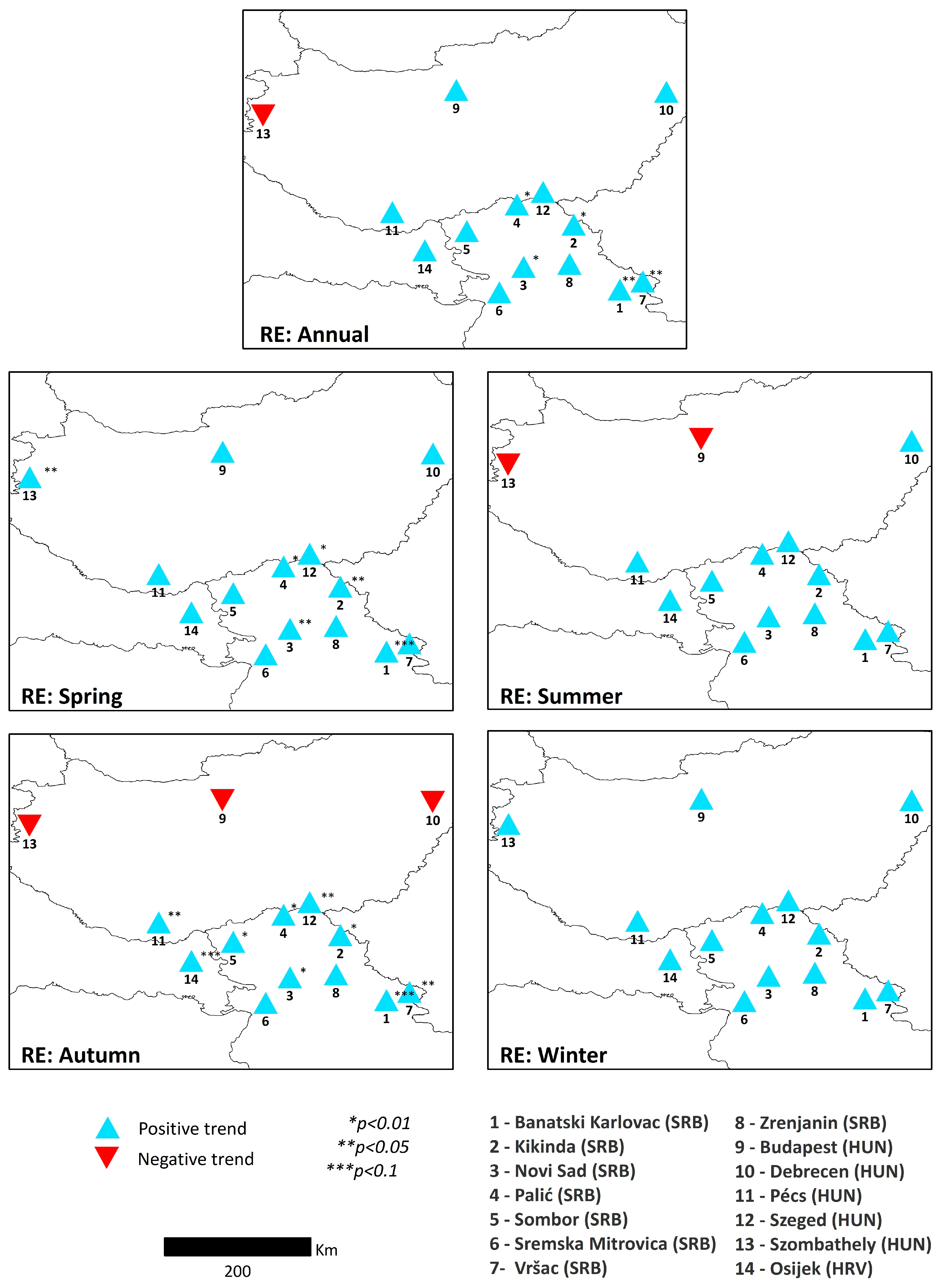
3.2.1. RE and ED Based on Station Data

The development of seasonal erosivity maps contributes to the estimation of the seasonal soil loss ratio [82]. Different seasonal spatial patterns of RE can be observed in Figure 5. During spring (March–May) and autumn (September–November), the study area is broadly divided into regions of higher RE in the southwest and lower RE in the northeast (Figure 5a,c). This gradient is less apparent during autumn, as Vojvodina (northern Serbia) has higher RE during autumn compared with spring. Both spring and autumn have high RE values (>400 MJ·mm·ha⁻¹·h⁻¹) in Osijek and Pécs, but the autumn maximum RE is in Szombathely (566 MJ·mm·ha⁻¹·h⁻¹). The lowest RE is seen in Budapest (128 MJ·mm·ha⁻¹·h⁻¹) in spring and Debrecen (226 MJ·mm·ha⁻¹·h⁻¹) in autumn.

As shown in Figure 4b, the highest seasonal RE values occur in summer. Following Figure 5b, two spatial clusters with higher RE (>700 MJ·mm·ha⁻¹·h⁻¹) can be seen. The first covers southwestern Hungary (Szombathely and Pécs) and Osijek in Eastern Croatia and the second one is located on the east end of Vojvodina (Vršac and Banatski Karlovac). The values of RE in the central part of the Pannonian Basin range between 400 and 700 MJ·mm·ha⁻¹·h⁻¹, except for Budapest, with an average of 260 MJ·mm·ha⁻¹·h⁻¹ during summer. Winter is the season with the smallest average RE (139 MJ·mm·ha⁻¹·h⁻¹) for the study area. South of the line Szombathely–Budapest–Debrecen RE values are >100 MJ·mm·ha⁻¹·h⁻¹, with the maximum in Osijek (217 MJ·mm·ha⁻¹·h⁻¹).

More than 70% of the annual RE in the central and southern Pannonian Basin occurs during the wet period, from April to October (Figure 6). It can be seen that the RE values in the eastern and western parts of the Pannonian Basin are larger than those in the northern and central parts. The lowest average monthly RE values are observed in February (33 MJ·mm·ha⁻¹·h⁻¹) and January (39 MJ·mm·ha⁻¹·h⁻¹), with the highest in June (285 MJ·mm·ha⁻¹·h⁻¹) and July (246 MJ·mm·ha⁻¹·h⁻¹). The monthly spatial patterns of RE, in general, display a continuous increase in RE from winter to spring, followed by a sharp high transition in the summer and a gradual decrease from autumn to winter. Identification of RE hotspots for specific times and places can guide investments in soil protection and help to avoid tillage during the most at-risk times [21]. However, it should be noted that extreme erosive rainfall events are not the only drivers of soil erosion. Other factors, such as topography, soil characteristics, and vegetation cover, also affect erosion rates, and, thus, should be addressed in future studies [31].

In the central and southern Pannonian Basin, the rainy season lasts from May to July, with high spatial variability in annual precipitation. Up to 1600 mm of annual rainfall can occur in the Ukrainian Carpathians and the Tatra Mountains, compared with 550 mm in the plains of eastern Hungary. The lowest summer precipitation is registered in northern Serbia (80 mm), while the lowest winter precipitation values are observed for northern Romania (70 mm) [83]. Increasing trends in total annual rainfall over the last 50 years have been reported for the region, except for northern Hungary [8].

Annual ED and RE follow the precipitation distribution with strong spatial variability (Figure 7a–c). High ED values (>3 MJ ha⁻¹ h⁻¹) indicate a greater risk of erosive rainstorms, soil erosion, and flooding [17,31,84]. The highest annual ED values for the study area are obtained for the southwest, in Osijek and Pécs (3.3 MJ ha⁻¹ h⁻¹), east in Debrecen (2.9 MJ ha⁻¹ h⁻¹), and southeast in Banatski Karlovac (2.8 MJ ha⁻¹ h⁻¹). Where ED values are >1, a certain precipitation amount may cause relatively higher RE. The lowest ED values occur in the northern (Budapest with 1.2 MJ ha⁻¹ h⁻¹) and central parts of the study area (e.g., Kikinda station in northern Vojvodina with 2.3 MJ ha⁻¹ h⁻¹). Regions with high ED are exposed to the risk of flooding and water scarcity as a result of their infrequent, but very intense and erosive, rainstorms [31].

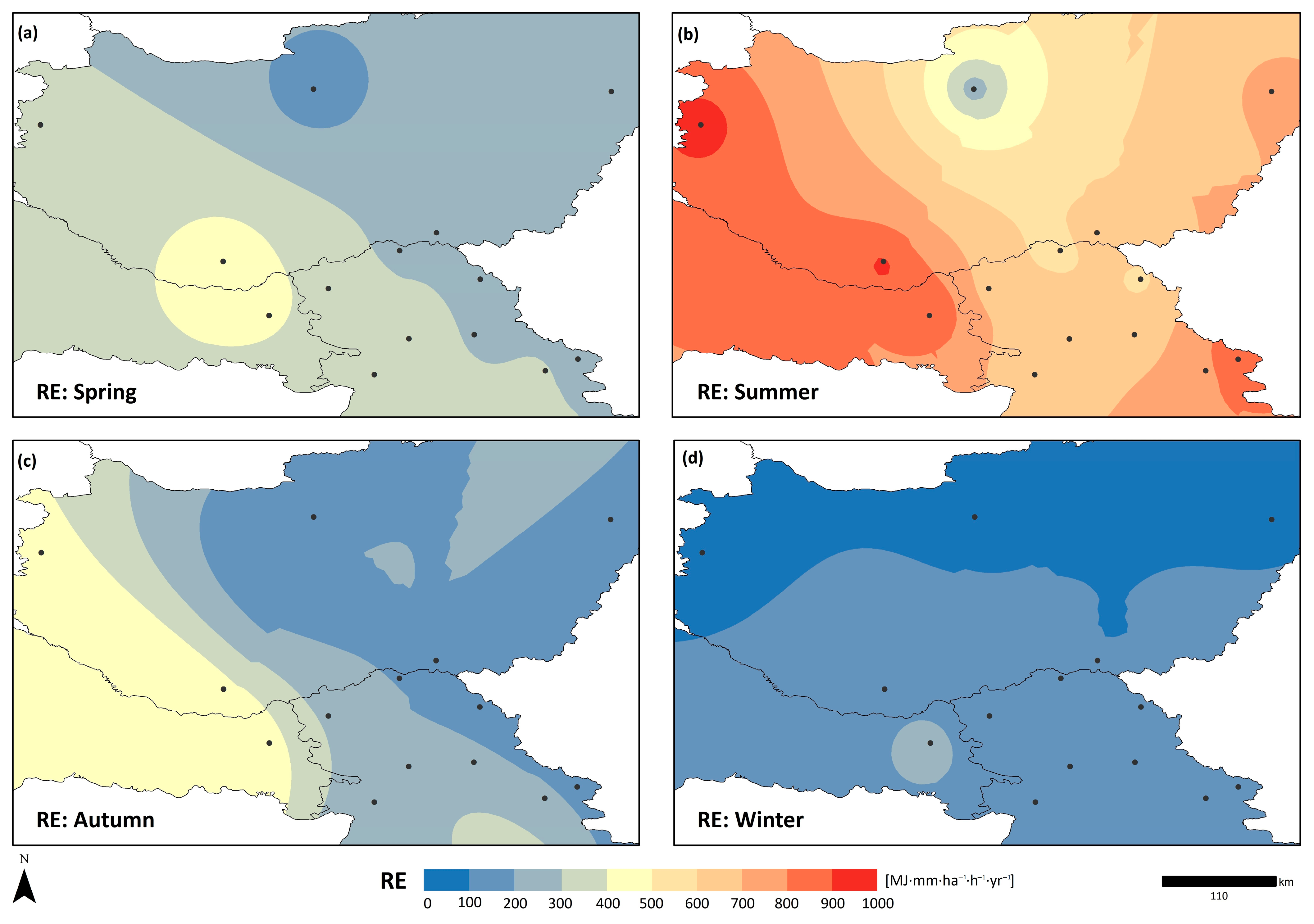
3.2.2. RE and ED Based on Gridded Data

The annual distribution of RE for the central and southern Pannonian Basin was also obtained for the gridded E-OBS datasets. The obtained result indicates good spatial agreement with the average annual precipitation for the investigated period (Figure 7d). The values are increasing from east to west, ranging from 250 MJ·mm·ha⁻¹·h⁻¹ (for the Great Hungarian Plain) to 2800 MJ·mm·ha⁻¹·h⁻¹ in the southwestern parts of Hungary (Figure 7e). The zones with the highest average ED (Figure 7f) correspond with the obtained RE values and range between 1.00 (the Great Hungarian Plain) and 3.75 MJ·ha⁻¹·h⁻¹ (Southern Transdanubia region and western parts of the Pannonian part of Croatia).

During the summer season, the RE exhibits its largest seasonal values for western parts of Hungary and the Pannonian part of Croatia (400–1000 MJ·mm·ha⁻¹·h⁻¹), as well as southeastern parts of the Vojvodina Region in northern Serbia (500–700 MJ·mm·ha⁻¹·h⁻¹) (Figure 8b). Higher RE values (from 300–800 MJ·mm·ha⁻¹·h⁻¹) are also observed for the autumn season in the western parts of the study area (Figure 8c).

The winter season exhibits relatively stable RE values ranging from 0 to 100 MJ·mm·ha⁻¹·h⁻¹ for the majority of the investigated area. The areas with higher RE values (varying between 100 and 200 MJ·mm·ha⁻¹·h⁻¹) are spotted in the southeastern and southwestern part of the study area (Figure 8d). These values are starting to divide into higher erosivity classes during the spring season (Figure 8a) following the previously observed spatial patterns extending from southeast to west (0–400 MJ·mm·ha⁻¹·h⁻¹).

The most erosive month is July, followed by June, August, and September. RE and ED are generally stable in the period from December to April, and then display an increase in values during the second period (Figure 9).

The performance of the spatial interpolation was validated by the root mean square error (RMSE) and standard error (SE) for both station and gridded RE values. RMSE is acceptable for the months that contribute to 70% of total RE (from May to September) (

Table 2. Performance of the spatial interpolation for each month, season and, annual RE.

Error	Monthly RE												Seasonal RE				Annual RE
	Jan	Feb	Mar	Apr	May	Jun	Jul	Aug	Sep	Oct	Nov	Dec	Spring	Summer	Autumn	Winter
SE station	2.60	1.36	1.49	0.37	3.10	11.67	1.49	−8.25	1.96	−2.96	0.65	2.99	4.66	−14.29	−19.87	8.88	46.33
SE grid	−0.09	−0.13	−0.18	−0.17	−0.30	−0.50	−0.62	−0.62	−0.50	−0.36	−0.24	−0.21	−0.57	−1.50	−0.95	−0.40	−3.28
RMSE station	21.42	8.09	16.99	14.00	53.97	66.15	81.88	65.90	46.52	24.47	17.39	17.78	76.13	201.90	104.73	36.80	323.85
RMSE grid	1.65	2.49	2.92	3.99	6.72	12.23	13.56	11.94	7.92	6.60	5.21	3.41	11.41	30.62	15.85	6.10	58.14

). It is expected that gridded data provide smaller errors due to much higher spatial resolution, as shown in Table 2. In combination with the SE, mean RE values can be used for estimating the intervals prediction.

4. Discussion

Spatial variations in annual precipitation, RE and ED, the R factor from Borrelli et al. [35], and FI and MFI of Lukić et al. [8] are compared in Figure 10. The spatial variations in R calculated by Borrelli et al. [35] partially coincide with RE station values obtained in this study. When comparing Figure 10b,d, it becomes evident that higher rainfall erosivity values are located in the southwest of the Pannonian Basin, but with deviation in rainfall erosivity values. In Figure 10d, Osijek meteorological station has an annual RE between 950 and 1000 MJ·mm·ha⁻¹·h⁻¹ [35], and, in Figure 10b, it falls in the last range between 2000 and 2150 MJ·mm·ha⁻¹·h⁻¹. The modelling results derived from the investigation of the changes in rainfall erosivity from Bezak et al. [25] (who used the COPERNICUS datasets and high-resolution erosive storms from the REDES database) indicate that the applied approach is showing a tendency to polish the annual erosivity values >1500 MJ·mm·ha⁻¹·h⁻¹.

Explanations for this deviation in rainfall erosivity estimates may be due to different (1) databases and spatial–temporal resolutions in the studies, and (2) methodologies applied for R factor calculation. The R factor was computed using sub-hourly (61%) and hourly pluviograph data (39%), obtained from the global rainfall–runoff erosivity database (GloREDa) from 2001 to 2012 [35], whereas the present study used daily data from the ECA&D database from 1961 to 2014. The methodology for computing the R factor was taken from the USDA RUSLE handbook and based on the Brown & Foster [84] equation for rainfall kinetic energy. In this study, RE distribution was computed by following [68] daily precipitation distributions. Since the European continental zone is characterised by warm summers and cold winters, it can be seen as an area prone to the high variability of RE. Due to this, and different methodological approaches, the mean RE values obtained in this study tend to be higher compared to the R factor for the Pannonian biogeographical region (660 MJ·mm·ha⁻¹·h⁻¹) [19]. Nonetheless, spatial patterns of the calculated indices are in relatively good agreement with other studies [19,35].

The work of Xie et al. [69] shows that there is a strong correlation between the power-law-derived relationship of empirical parameters α and β (within the Zhang et al. [68] RE model). However, mainly β was associated with average daily ($\overline{P}$_d12) and annual erosive rainfall ($\overline{P}$_y12). These parameters can be significantly linearly related with the mean annual rainfall (as the independent variable), yet, on other occasions, display insignificant linearity. Yu [36] and Xie et al. [69] explained this in terms of the aggregation of the above-mentioned parameters, which were obtained month by month (in their respective studies), and by all months, as presented by Zhang et al. [68] and this study. If parameter β is not properly estimated, the deviation of the model output may occur. Hence, Xie et al. [69] indicated that one of the reasons for the overestimation when using the Zhang et al. [68] model may be attributed to the utilisation of a surrogate for the measured value of EI₃₀. In this model, the surrogate was perceived as the product of daily rainfall P_d and the maximum 10-min intensity in a day I_10d, multiplied by a conversion factor of 0.184. Although Xie et al. [69] observed that daily rainfall and maximum 10-min intensity in a day are highly correlated, the use of P_d I_10d instead of EI₃₀ (due to data scarcity) contributes to the uncertainty of this relationship. Therefore, the results in this study emphasise that there is a great necessity for a more proper calibration for this model to be implemented in other places.

Yang and Yu [37] outlined that rainfall erosivity can vary depending on the time of year and location, especially when it comes to latitude and elevation. On the other hand, the RUSLE manual states that the R factor is mainly quantified using a defined threshold rainfall amount of 12.7 mm [85]. The observed discrepancies in the obtained R factor can be due to different rainfall thresholds (used here and in other European studies), thus leading to the increased values, as mean annual rainfall decreases because the relative contribution of small storm events is greater in dry areas.

When it comes to the contemporary analysis of the spatiotemporal rainfall erosivity and its variability in Europe, Bezak et al. [31] highlighted that the regional temporal RE patterns do not display homogenous behaviour due to the relatively large differences among neighbouring meteorological stations, and also the sparse network is problematic and places a lot of dependence on the choice of interpolation technique. This leads to the conclusion that local climatological conditions determine the local temporal rainfall erosivity distribution, as seen in this work (some meteorological stations can show the similar temporal distribution of RE and ED while having quite different absolute RE and ED values). Bezak et al. [31] explained this pattern by the differences between rainfall erosivity synchrony scale (Rsync) and computed precipitation synchrony scale. Rsync is the maximum radius (in km) surrounding a meteorological station where at least half of the other meteorological stations record an erosive event.

When observing the assessment of rainfall energy, the FI and MFI results gained by Lukić et al. [8] should be discussed, as they have very good correspondence with RE spatial distribution in this study. According to respective authors, the central and southern Pannonian Basin area belongs to the erosive class of low values (20–47), with the tendencies of a progressive increase in the values of the erosion index at the annual level, hence leading to the possible transition to a higher erosive class and increase in the sensitivity to erosion by water processes in the given area (Figure 10e,f). According to these indices, the majority of the study area belongs to the low erosivity class, except in the northwest, which, in the future, could lead to a transition to a higher erosion category related to RE variation for this part of the Pannonian Basin.

On the other hand, climate gridded datasets are valuable and useful when performing detailed analysis of RE and ED at regional scales. As highlighted by Sidău et al. [86], usage of such data is important for the development of quality results that can be used as tools for climate services, policies, and strategies for climate change adaptation and mitigation. Obtained results correspond quite well with the results of Panagos et al. [19], who used data from 42 stations from Croatia and 30 from Hungary for the period 1961–2012 and 1998–2013, respectively. Respective authors argued that, on the country level, one of the highest calculated values of the R factor is observed for Austria and Croatia (mean values of >1000 MJ·mm·ha⁻¹·h⁻¹). In this study, it has been found that values for the Pannonian part of Croatia are increasing from east to west (ranging from 750 to 2800 MJ·mm·ha⁻¹·h⁻¹). Possible reasons for the difference in R factor variability between the studies could have occurred due to data availability, analysed period, data quality, sample sizes, interpolation method, and interpretation. An overall increase in the mean R factor for our study can be seen in the most western parts of the investigated area. This feature could have been influenced by the availability of long-term rainfall data with better temporal resolution from a higher number of weather stations and a denser spatial distribution than previous studies [19,20]. Moreover, respective authors [19] produced R factors of different temporal resolutions to 30-min resolution by applying a calibration factor for comparability of data from the study area. This approach may have caused a certain decrease in obtained R factors for Croatia and Hungary. Generally speaking, Mehr et al. [87] highlighted that observed trends for Osijek meteorological station (eastern part of Croatia) could pose a danger to regional agricultural production, and thus should be addressed with special attention when analysing the emergence of new climate extremes over the territory of the Pannonian Basin. Pásztor et al. [88] used the Pan-European Soil Erosion Risk Assessment (PESERA) model to perform rill and inter-rill erosion estimates at the regional level due to the lack of available in situ soil erosion datasets in Hungary. The authors identified high erosion rates in mountainous and hilly areas in the northern parts of Hungary and the southern Transdanubia region, highlighting that more than 26% of the country’s total area is susceptible to moderate and high erosion rates. This was also the case for the extremely wet year of 2010, where R factor varied between 2300 and 3400 MJ·mm·ha⁻¹·h⁻¹. Results from our study highlight that the above-mentioned areas experience rainfall erosivity ranging between 500 and 2800 MJ·mm·ha⁻¹·h⁻¹, thus corresponding well with the previous study. The Great Hungarian Plain generally exibits low erosion rates (250–500 MJ·mm·ha⁻¹·h⁻¹), with a few regions where mostly sandy soils dominate [88]. The high extent of the lowland areas is, therefore, affected only by relatively low erosion rates, while, on the other hand, significantly higher erosion rates can be seen in the hills and mountains. For northern Serbia (Vojvodina), variability of calculated RE values display certain contrasts between lowland (500–750 MJ·mm·ha⁻¹·h⁻¹) and mountainous/hilly areas, which exibit the highest susceptibility to rainfall erosivity during the observed period of 1961–2014 (1000–1250 MJ·mm·ha⁻¹·h⁻¹). These results are in good agreement with the study of Lukić et al. [61], who outlined that highest rainfall erosivity values can be seen for southeastern parts of the Vojvodina Region (Banat Region with Vršac weather station). Authors also emphasised that, as the altitude decreases, severe and very severe erosivity class values are approximately equally distributed on a multiannual basis. Since this study revealed that the highest average ED corresponds with the obtained RE values, it can be stated that RE is driven by rainfall intensity in the investigated period. Obtained results are in agreement with the findings of Panagos et al. [19]. The authors of this study state that the combination of higher values of RE and ED could lead to various environmental risks when high rainfall amounts falling on moist or saturated soils could trigger landslide events or wetland erosion, thus intensifying soil degradation processes. Within the study area, differences in the seasonal patterns of rainfall erosivity can be seen. With the summer season displaying the highest RE values in western parts of Hungary, the Pannonian part of Croatia, and southeastern parts of the Vojvodina Region in northern Serbia, it can be highlighted that these findings correspond well with the distribution of the seasons with the largest R factor values provided by Panagos et al. [21]. Moreover, further results follow the findings of the mentioned authors who distinguish a second RE zone, with the autumn being the second most erosive period, including parts of Croatia (200–900 MJ·mm·ha⁻¹·h⁻¹). These observations support the statement that the R factor is highest during the summer season in central Europe due to large-scale extreme precipitation events [32]. Similar patterns can be seen in northern Serbia, where Milovanović et al. [89] indicated that increases in June precipitation amounts reach up to 3 mm/decade (with small areas increasing up to 8 mm/decade, respectively). The findings from this study follow the values presented on monthly erosivity maps of Europe (for January and July) by Panagos et al. [32]. Therefore, as the magnitude of the predicted climate change is likely to have a pronounced influence on water erosion processes, investigation of regional conditions that influence RE and ED is of great importance for future studies. The results of this research clearly outline the importance of the utilisation of quality gridded datasets in research activities related to the estimation of rainfall erosivity on a regional scale. On the other hand, considering the variables of daily precipitation, the E-OBS dataset displays a certain underestimation of the precipitation magnitude in the Pannonian (Carpathian) region. Hence, the investigation of the long-term trends should be performed exclusively on weather station data due to temporal inconsistencies within gridded datasets caused by residual inhomogeneities in the used station network [89].

4.1. Long-Term Trends of Annual and Seasonal RE and ED

Long-term trends in the annual and seasonal RE for each meteorological station were examined with the M–K test method and are shown in Figure 11. It can be seen that annual RE has a generally positive trend for every station, except for Szombathely (in the western part of Hungary). However, Szeged in the south of Hungary has a positive trend (p < 0.01). Four meteorological stations with statistically significant trends are located in Vojvodina, with two stations displaying rising tendencies detected for the confidence level of 99% (p < 0.01) and two stations for the confidence level of 95% (p < 0.05). Spring RE values have increasing trends for all stations, of which 5/14 stations have statistically significant results: Szeged and Palić at the confidence level of 99% (p < 0.01), Kikinda, Novi Sad, and Szombathely at the confidence level of 95% (p < 0.05), and Banatski Karlovac at the confidence level of 90% (p < 0.1). Summer and winter season trends of RE (with the exception of Budapest and Szombathely) display an increase, but without statistical significance at the specified confidence levels. Autumn has an increasing trend for RE values in Vojvodina and eastern Croatia, with a statistical significance of 99% (p < 0.01) and 95% (p < 0.05) for three stations, and two stations with a statistical significance of 90% (p < 0.1). For the rest of Hungary, except Szeged, the autumn RE trend is decreasing. These long-term seasonal trends are in line with the results of Tošić et al. [74] for the territory of Vojvodina, as they found an increasing trend for autumn and annual precipitation. Bezak et al. [25] also reported an increasing trend for most parts of the Pannonian Basin by using the M–K test, emphasising statistical significance for central Hungary (p < 0.02), northwestern Vojvodina (from p < 0.06 to p < 0.16), the rest of Vojvodina, and eastern Croatia (p < 0.17–p < 0.28).

Figure 12 shows long-term trends in the annual and seasonal ED spatial distribution. With the observation of statistical significance for positive annual trend, it can be seen that Szeged station in southern Hungary has p < 0.01, while three stations in Vojvodina have a positive trend with the statistical significance of 95% (p < 0.1) and one with 90% (p < 0.1). Other stations all have increasing trends, but without statistical significance, except Szombathely, which has a negative trend (without statistical significance). Spring and autumn seasons have similar spatial distribution for positive and negative trend distribution (Figure 12). During the spring, a rising trend is recorded with a confidence level of 99% for two stations, 95% for three stations, and 90% confidence level for one station. A negative ED trend is recorded during spring in the western part of Hungary (Szombathely station), with a confidence level of 95%. Both summer and winter ED trend distribution are without the presence of statistical significance (Figure 12). Panagos et al. [19] highlighted a necessity for a joint assessment of the ED and the risk areas in areas with the combination of low precipitation and high ED values (central Hungary), as well as medium-high precipitation with medium-high ED values (western Hungary and eastern Croatia). These results show that parts of the Pannonian Basin are at high risk of erosive events, as well as from water scarcity and floods [14,19].

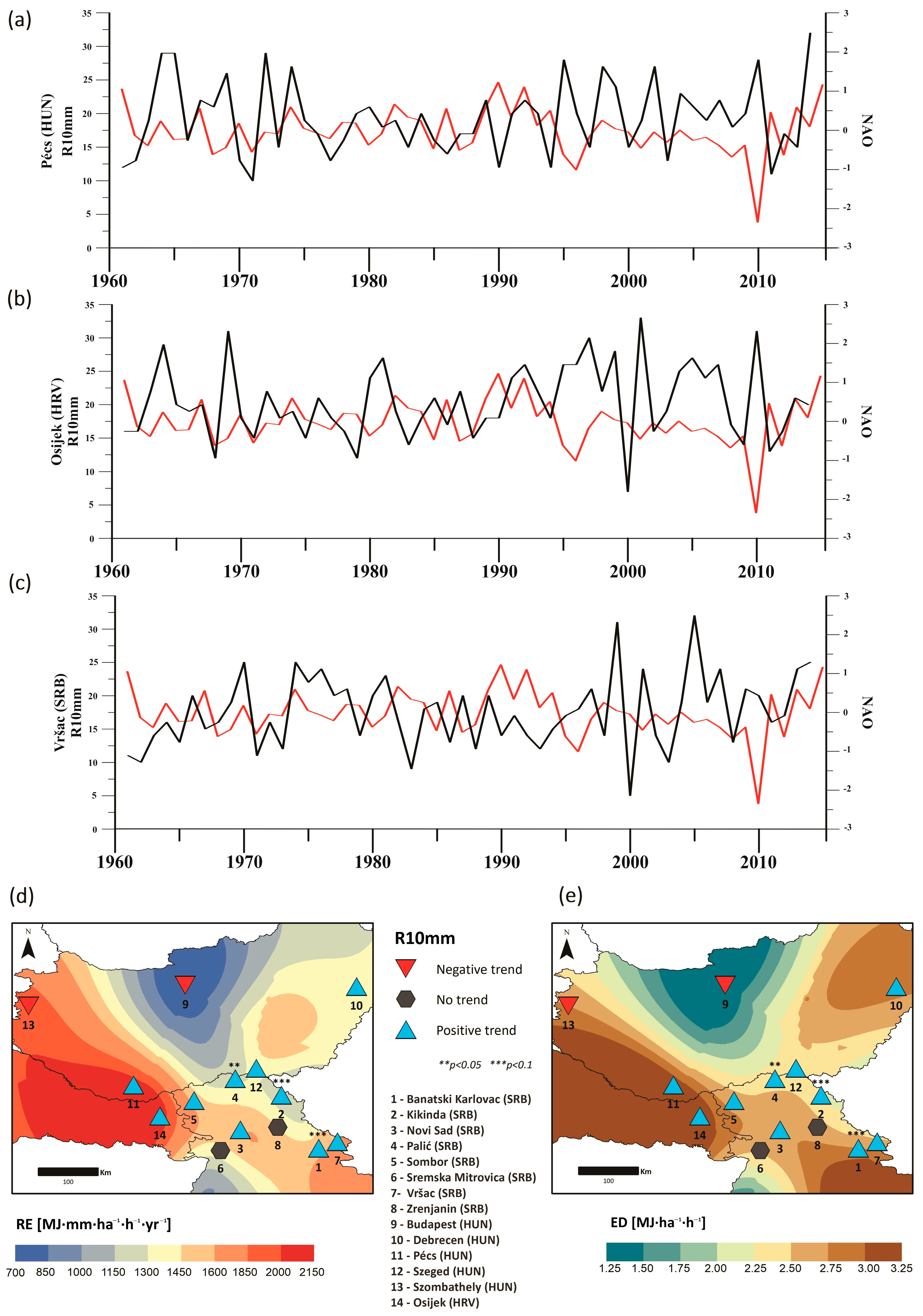
4.2. North Atlantic Oscillation Impact

Large-scale atmospheric circulation patterns have a considerable impact on precipitation variability [90]. As shown by Dehghani et al. [91], these patterns have a considerable impact on precipitation in different regions, where various climate indices in different phases may decrease the seasonal precipitation (even up to 100%). On the other hand, seasonal precipitation may increase >100% in different seasons due to the impact of these indices.

Many recent studies [61,76,77,92] have highlighted that North Atlantic Oscillation (NAO) has a prominent impact on the rainfall amount, and, since RE and ED are based on precipitation amounts, NAO has a certain influence on them as well. As highlighted by Bice et al. [90], NAO has a strong influence on winter precipitation in the Pannonian Basin, with negative NAO phases corresponding to periods of high precipitation. This is consistent with winter RE trend values obtained in this study (Figure 11).

Other respective authors also argued that the regional intensity and frequency of extreme precipitation increased during the period between 1976 and 2001 [8,93], while total precipitation decreased. The increasing occurrence of the precipitation extremes in this part of the Pannonian Basin characterises the climate of the region as drier in the summer and wetter during the winter season. Other studies indicate that the amount and intensity of precipitation in Serbia have significantly increased during autumn in the Vojvodina (northern Serbia) [94]. It has been shown that the climate of southern parts of the Pannonian Basin has become wetter during the last 50 years, regarding the precipitation magnitude and its frequency [8,94].

The study of Lukić et al. [8] indicated that the number of heavy precipitation days (R10mm) is increasing, with varying degrees of statistical significance at only three stations in the southeastern part of the study area (Banatski Karlovac, Kikinda, and Palić meteorological stations). This extreme precipitation index is in good agreement with the annual spatial distribution of RE and ED values (Figure 13d,e) since the used Zhang et al. [68] model includes the erosive rainfall values when the actual rainfall was >12 mm. Moreover, from Figure 13, it can be seen that this variability is strongly influenced by NAO when observing the southern stations from the investigated area (Figure 13a–c), with negative NAO phases corresponding to periods of high precipitation.

Correlation coefficients between the NAO and R10mm indices were determined in order to investigate the possible relationships between RE/ED and atmospheric variability. Results are shown in

Table 3. Pearson correlation test (r) results of NAO and R10mm.

Station Name	NAO
	Annual	Spring	Summer	Autumn	Winter
Banatski Karlovac	−0.23	0.04	−0.20	−0.09	−0.19
Kikinda	−0.36 **	0.02	−0.26	−0.13	−0.34 *
Novi Sad	−0.18	0.19	−0.13	−0.15	−0.23
Palić	−0.37 **	−0.05	−0.23	−0.22	−0.27
Sombor	−0.20	0.11	−0.12	−0.10	−0.26
Sremska Mitrovica	−0.20	0.14	−0.11	0.01	−0.36 **
Vršac	−0.13	0.03	−0.13	0.01	−0.15
Zrenjanin	−0.32 *	0.03	−0.18	−0.01	−0.42 **
Budapest	−0.23	−0.08	−0.01	−0.12	−0.24
Debrecen	−0.31 *	−0.06	−0.12	−0.08	−0.34 *
Pécs	−0.21	0.02	−0.10	−0.29 *	−0.09
Szeged	−0.30 *	−0.07	−0.11	−0.12	−0.29 *
Szombathely	0.07	0.16	0.12	0.02	−0.09
Osijek	−0.28 *	0.02	−0.08	−0.22	−0.27 *

**—correlation is significant at the 0.01 level; *—correlation is significant at the 0.05 level. Blue: negative correlation; red: positive correlation.

. The correlation between the analysed indices is significant (at a 99% and 95% level of significance) for six weather stations at the annual level. Weather stations such as Kikinda and Palić (northern Serbia) have a significant correlation with values varying between −0.36 and −0.37 at the 99% level of significance. On the other hand, meteorological stations Osijek (eastern Croatia), Szeged, and Debrecen (Hungary), as well as Zrenjanin (northern Serbia), display a significant correlation varying between −0.28 and −0.32 at the 95% level of significance. The correlation between the NAO and R10mm index is significant only for Pécs meteorological station (−0.29 at a 95% level of significance) for the autumn season. The winter season displays strong linearity between the observed indices for Sremska Mitrovica and Zrenjanin (values varying between −0.36 and −0.42 at the 99% level of significance) in northern Serbia. Analysed stations, such as Osijek, Szeged, Debrecen, and Kikinda, have a significant correlation varying between −0.27 and −0.34 at the 95% level of significance. Obtained results correlate well with the findings of Lukic et al. [61], who emphasised that the negative correlation coefficient could indicate the wetting effect on the RE and ED parameters.

According to the findings of Lukić et al. [8], the annual total precipitation (when it exceeds the 95th percentile (R95p)) is increasing in the investigated area, except for the Budapest meteorological station. Ossó et al. [95] revealed that from 2000 to 2016, annual values of the R95p index were 5% larger in central Europe. The authors stated that, during the winter season, R95p was positive for most of Europe, thus leading to unusually intense winter precipitation. These results are in good agreement with spatio–temporal distribution of RE and ED obtained in this study, indicating that very wet days significantly contribute to the increase in extreme rainfall events and rainfall erosivity rates in general (Figure 14a,b).

Generally speaking, the calculated increasing trends in RE are in good agreement with this pattern on both annual and seasonal scales. Positive spring and autumn trends of RE can be the result of an increase in the amount of precipitation in short periods, as well as due to an increase in the contribution of extreme events to the total amount of precipitation. Moreover, ED is influenced not only by NAO but also by the East Atlantic/West Russia (EAWR) patterns in terms of intensity of precipitation and the frequency of dry and wet conditions [94]. Future research should be oriented towards the investigation of large-scale atmospheric processes, as drivers of the seasonal erosivity over the central and southern Pannonian Basin. Such research should explore the relationship between the above-mentioned large-scale processes of climate variability, their impact on changes in seasonal precipitation, and thus associated erosivity values. This approach would enable links to be made between seasonal outlooks of circulation indices (such as NAO) and heightened/lowered risk of soil erosion across the region. Similarly, the same atmospheric, rainfall, and erosion indices could be derived from climate model output to assess future risks of soil loss under climate change.

5. Conclusions

Estimation of rainfall erosivity and density is important for the understanding of the climate vulnerability in the region. Analysis of RE and ED for the central and southern Pannonian Basin was performed, complemented by seasonal trend and spatial variability analyses for the period of 1961–2014. The findings show seasons and hotspots with high erosion risks that are relevant to the development of prevention activities and promotion of suitable mitigation measures at local to regional scales.

Results in this study represent only a piece in the mosaic of spatio–temporal rainfall erosivity variability in Europe. Different periods, meteorological stations, and temporal resolution of data can yield differences in erosion risk indices for this part of the Pannonian Basin. The methodology used in the present study with the usage of station observations and gridded datasets display certain discrepancies when it comes to extremely high erosive events. The annual RE and ED are following the precipitation distribution patterns with a strong spatial variability: higher values are observed for southwestern and southeastern parts; minimal values dominate over north and northeastern parts. Detected trends obtained for weather stations indicate a general increase in RE and ED at the annual level, as well as during the spring and autumn seasons. This increase may cause a transition to a higher erosive class in the near future by elevating the vulnerability for this type of hydro-meteorological hazard in the central and southern Pannonian Basin. This study confirmed the importance of NAO atmospheric circulation by observing its correlation with the number of heavy precipitation days. During the winter season, as well as on an annual scale, significant correlations (for the given confidence levels) are observed, thus indicating the possible wetting effects on the RE and ED parameters.

Despite the use of high-resolution data (E-OBS), extreme erosive events can influence the mean annual RE and ED and, thus, their probability of occurrence needs to be accounted for in future regional studies. However, this study largely enhances previously performed analysis that was focused solely on the assessment of the distribution, concentration, variability of precipitation, and rainfall aggressiveness as the contributing factors in the triggering or reactivation of erosion phenomena in this part of Europe.

The results of this work contribute to growing evidence of erosion risk in southeast Europe and have scope for further refinements. This is especially referring to the territory of northern Serbia (Vojvodina Region) and other Western Balkan countries not intensively covered by previous studies. Future work should be oriented towards the usage of daily rainfall erosivity models with regionalised parameters (in particular α and β, since they are closely related to climate characteristics and the topography of the given location). A greater density of meteorological stations or gridded datasets of high spatial resolution (e.g., ERA5, 0.1 deg.), length of the observation period, and RE model based on RUSLE guidelines could ensure quality regional model parameters. However, one should bear in mind the somewhat existing limitations of the model (limited interactions between input factors, lack of deposition of sediment prediction, model upscaling issues, etc.) and future utilisation of more sensitive indices, along with physically based models for estimating soil erosion rates (e.g., RUSLE, RUSLE₂), could help to fill in the gaps in the rainfall erosivity map of Europe. Analysis of the REDES database could enable a more suitable comparison of the results aggregated with the usage of the above-mentioned methodologies. This approach would allow a more dynamic soil erosion assessment and identification of extreme erosive events on both local and regional scales affected by climate change impacts.

References

1. Nasidi, N.M.; Wayayok, A.; Abdullah, A.F.; Kassim, M.S.M. Spatio-temporal dynamics of rainfall erosivity due to climate change in Cameron Highlands, Malaysia. Model. Earth Syst. Environ. 2021, 7, 1847–1861. [Google Scholar] [CrossRef]
2. Azari, M.; Oliaye, A.; Nearing, M.A. Expected climate change impacts on rainfall erosivity over Iran based on CMIP5 climate models. J. Hydrol. 2021, 593, 125826. [Google Scholar] [CrossRef]
3. Borrelli, P.; Robinson, D.A.; Panagos, P.; Lugato, E.; Yang, J.E.; Alewell, C.; Wuepper, D.; Montanarella, L.; Ballabio, C. Land use and climate change impacts on global soil erosion by water (2015–2070). Proc. Natl. Acad. Sci. USA 2020, 117, 21994–22001. [Google Scholar] [CrossRef] [PubMed]
4. Zeder, J.; Fischer, E.M. Observed extreme precipitation trends and scaling in Central Europe. Weather Clim. Extrem. 2020, 29, 100266. [Google Scholar] [CrossRef]
5. Hamouda, M.E.; Pasquero, C. European extreme precipitation: The effects of spatio-temporal resolution of the data. Weather Clim. Extrem. 2021, 33, 100337. [Google Scholar] [CrossRef]
6. Dar, J.; Nabi, S.; Dar, A.Q.; Ahanger, M.A. The anatomy of extreme precipitation events over Srinagar, Kashmir, India, over the past 50 years. Arab. J. Geosci. 2021, 14, 1412. [Google Scholar] [CrossRef]
7. Boardman, J.; Poesen, J. Soil Erosion in Europe; Boardman, J., Poesen, J., Eds.; John Wiley & Sons, Ltd.: Chichester, UK, 2006; ISBN 9780470859209. [Google Scholar]
8. Lukić, T.; Lukić, A.; Basarin, B.; Ponjiger, T.M.; Blagojević, D.; Mesaroš, M.; Milanović, M.; Gavrilov, M.; Pavić, D.; Zorn, M.; et al. Rainfall erosivity and extreme precipitation in the Pannonian basin. Open Geosci. 2019, 11, 664–681. [Google Scholar] [CrossRef]
9. Grillakis, M.G.; Polykretis, C.; Alexakis, D.D. Past and projected climate change impacts on rainfall erosivity: Advancing our knowledge for the eastern Mediterranean island of Crete. Catena 2020, 193, 104625. [Google Scholar] [CrossRef]
10. Chen, Y.; Xu, M.; Wang, Z.; Chen, W.; Lai, C. Reexamination of the Xie model and spatiotemporal variability in rainfall erosivity in mainland China from 1960 to 2018. Catena 2020, 195, 104837. [Google Scholar] [CrossRef]
11. Xu, Z.; Pan, B.; Han, M.; Zhu, J.; Tian, L. Spatial–temporal distribution of rainfall erosivity, erosivity density and correlation with El Niño–Southern Oscillation in the Huaihe River Basin, China. Ecol. Inform. 2019, 52, 14–25. [Google Scholar] [CrossRef]
12. Telles, T.S.; Guimarães, M.d.F.; Dechen, S.C.F. The costs of soil erosion. Rev. Bras. Ciência Do Solo 2011, 35, 287–298. [Google Scholar] [CrossRef]
13. Boardman, J.; Vandaele, K.; Evans, R.; Foster, I.D.L. Off-site impacts of soil erosion and runoff: Why connectivity is more important than erosion rates. Soil Use Manag. 2019, 35, 245–256. [Google Scholar] [CrossRef] [Green Version]
14. Mihailović, D.T.; Lalić, B.; Drešković, N.; Mimić, G.; Djurdjević, V.; Jančić, M. Climate change effects on crop yields in Serbia and related shifts of Köppen climate zones under the SRES-A1B and SRES-A2. Int. J. Climatol. 2015, 35, 3320–3334. [Google Scholar] [CrossRef]
15. Padulano, R.; Rianna, G.; Santini, M. Datasets and approaches for the estimation of rainfall erosivity over Italy: A comprehensive comparison study and a new method. J. Hydrol. Reg. Stud. 2021, 34, 100788. [Google Scholar] [CrossRef]
16. Morar, C.; Lukić, T.; Basarin, B.; Valjarević, A.; Vujičić, M.; Niemets, L.; Telebienieva, I.; Boros, L.; Nagy, G. Shaping Sustainable Urban Environments by Addressing the Hydro-Meteorological Factors in Landslide Occurrence: Ciuperca Hill (Oradea, Romania). Int. J. Environ. Res. Public Health 2021, 18, 5022. [Google Scholar] [CrossRef]
17. Li, X.; Ye, X. Variability of Rainfall Erosivity and Erosivity Density in the Ganjiang River Catchment, China: Characteristics and Influences of Climate Change. Atmosphere 2018, 9, 48. [Google Scholar] [CrossRef] [Green Version]
18. Yin, S.; Nearing, M.A.; Borrelli, P.; Xue, X. Rainfall Erosivity: An Overview of Methodologies and Applications. Vadose Zone J. 2017, 16, vzj2017.06.0131. [Google Scholar] [CrossRef] [Green Version]
19. Panagos, P.; Ballabio, C.; Borrelli, P.; Meusburger, K.; Klik, A.; Rousseva, S.; Tadić, M.P.; Michaelides, S.; Hrabalíková, M.; Olsen, P.; et al. Rainfall erosivity in Europe. Sci. Total Environ. 2015, 511, 801–814. [Google Scholar] [CrossRef] [Green Version]
20. Panagos, P.; Borrelli, P.; Poesen, J.; Ballabio, C.; Lugato, E.; Meusburger, K.; Montanarella, L.; Alewell, C. The new assessment of soil loss by water erosion in Europe. Environ. Sci. Policy 2015, 54, 438–447. [Google Scholar] [CrossRef]
21. Panagos, P.; Ballabio, C.; Borrelli, P.; Meusburger, K. Spatio-temporal analysis of rainfall erosivity and erosivity density in Greece. Catena 2016, 137, 161–172. [Google Scholar] [CrossRef]
22. Panagos, P.; Katsoyiannis, A. Soil erosion modelling: The new challenges as the result of policy developments in Europe. Environ. Res. 2019, 172, 470–474. [Google Scholar] [CrossRef]
23. Panagos, P.; Ballabio, C.; Himics, M.; Scarpa, S.; Matthews, F.; Bogonos, M.; Poesen, J.; Borrelli, P. Projections of soil loss by water erosion in Europe by 2050. Environ. Sci. Policy 2021, 124, 380–392. [Google Scholar] [CrossRef]
24. Borrelli, P.; Alewell, C.; Alvarez, P.; Anache, J.A.A.; Baartman, J.; Ballabio, C.; Bezak, N.; Biddoccu, M.; Cerdà, A.; Chalise, D.; et al. Soil erosion modelling: A global review and statistical analysis. Sci. Total Environ. 2021, 780, 146494. [Google Scholar] [CrossRef]
25. Bezak, N.; Ballabio, C.; Mikoš, M.; Petan, S.; Borrelli, P.; Panagos, P. Reconstruction of past rainfall erosivity and trend detection based on the REDES database and reanalysis rainfall. J. Hydrol. 2020, 590, 125372. [Google Scholar] [CrossRef]
26. Bezak, N.; Borrelli, P.; Panagos, P. A first assessment of rainfall erosivity synchrony scale at pan-European scale. Catena 2021, 198, 105060. [Google Scholar] [CrossRef]
27. Mello, C.R.; Viola, M.R.; Beskow, S.; Norton, L.D. Multivariate models for annual rainfall erosivity in Brazil. Geoderma 2013, 202–203, 88–102. [Google Scholar] [CrossRef]
28. Wishmeier, W.H.; Smith, D.D. Predicting Rainfall Erosion Losses—A Guide to Conservation Planning, 537th ed.; United States Department of Agriculture, Science and education administration: Hyattsville, MD, USA, 1978. [Google Scholar]
29. Wilby, R.L.; Yu, D. Rainfall and temperature estimation for a data sparse region. Hydrol. Earth Syst. Sci. 2013, 17, 3937–3955. [Google Scholar] [CrossRef] [Green Version]
30. Zhu, D.; Xiong, K.; Xiao, H. Multi-time scale variability of rainfall erosivity and erosivity density in the karst region of southern China, 1960–2017. Catena 2021, 197, 104977. [Google Scholar] [CrossRef]
31. Bezak, N.; Mikoš, M.; Borrelli, P.; Liakos, L.; Panagos, P. An in-depth statistical analysis of the rainstorms erosivity in Europe. CATENA 2021, 206, 105577. [Google Scholar] [CrossRef]
32. Panagos, P.; Borrelli, P.; Spinoni, J.; Ballabio, C.; Meusburger, K.; Beguería, S.; Klik, A.; Michaelides, S.; Petan, S.; Hrabalíková, M.; et al. Monthly Rainfall Erosivity: Conversion Factors for Different Time Resolutions and Regional Assessments. Water 2016, 8, 119. [Google Scholar] [CrossRef] [Green Version]
33. Polade, S.D.; Gershunov, A.; Cayan, D.R.; Dettinger, M.D.; Pierce, D.W. Precipitation in a warming world: Assessing projected hydro-climate changes in California and other Mediterranean climate regions. Sci. Rep. 2017, 7, 10783. [Google Scholar] [CrossRef] [PubMed] [Green Version]
34. IPCC. Climate Change and Land: An IPCC Special Report. Available online: https://spiral.imperial.ac.uk/bitstream/10044/1/76618/2/SRCCL-Full-Report-Compiled-191128.pdf (accessed on 1 October 2021).
35. Borrelli, P.; Robinson, D.A.; Fleischer, L.R.; Lugato, E.; Ballabio, C.; Alewell, C.; Meusburger, K.; Modugno, S.; Schütt, B.; Ferro, V.; et al. An assessment of the global impact of 21st century land use change on soil erosion. Nat. Commun. 2017, 8, 2013. [Google Scholar] [CrossRef] [PubMed] [Green Version]
36. Yu, B. Rainfall erosivity and its estimation for Australia’s tropics. Soil Res. 1998, 36, 143. [Google Scholar] [CrossRef]
37. Yang, X.; Yu, B. Modelling and mapping rainfall erosivity in New South Wales, Australia. Soil Res. 2015, 53, 178. [Google Scholar] [CrossRef]
38. Klik, A.; Haas, K.; Dvorackova, A.; Fuller, I.C. Spatial and temporal distribution of rainfall erosivity in New Zealand. Soil Res. 2015, 53, 815. [Google Scholar] [CrossRef]
39. Meshesha, D.T.; Tsunekawa, A.; Tsubo, M.; Haregeweyn, N.; Adgo, E. Evaluating spatial and temporal variations of rainfall erosivity, case of Central Rift Valley of Ethiopia. Theor. Appl. Climatol. 2015, 119, 515–522. [Google Scholar] [CrossRef]
40. Meddi, M.; Toumi, S.; Assani, A.A. Spatial and temporal variability of the rainfall erosivity factor in Northern Algeria. Arab. J. Geosci. 2016, 9, 282. [Google Scholar] [CrossRef]
41. Fenta, A.A.; Yasuda, H.; Shimizu, K.; Haregeweyn, N.; Kawai, T.; Sultan, D.; Ebabu, K.; Belay, A.S. Spatial distribution and temporal trends of rainfall and erosivity in the Eastern Africa region. Hydrol. Process. 2017, 31, 4555–4567. [Google Scholar] [CrossRef]
42. da Silva, A.M. Rainfall erosivity map for Brazil. CATENA 2004, 57, 251–259. [Google Scholar] [CrossRef]
43. Almagro, A.; Oliveira, P.T.S.; Nearing, M.A.; Hagemann, S. Projected climate change impacts in rainfall erosivity over Brazil. Sci. Rep. 2017, 7, 8130. [Google Scholar] [CrossRef] [Green Version]
44. Avila Rangel, H.F.; Avila Rangel, B.D. Spatial and temporal estimation of the erosivity factor R based on daily rainfall data for the department of Atlántico, Colombia. Ing. Investig. 2015, 35, 23–29. [Google Scholar] [CrossRef]
45. Lee, J.-H.; Heo, J.-H. Evaluation of estimation methods for rainfall erosivity based on annual precipitation in Korea. J. Hydrol. 2011, 409, 30–48. [Google Scholar] [CrossRef]
46. Shin, J.-Y.; Kim, T.; Heo, J.-H.; Lee, J.-H. Spatial and temporal variations in rainfall erosivity and erosivity density in South Korea. CATENA 2019, 176, 125–144. [Google Scholar] [CrossRef]
47. Sadeghi, S.H.; Zabihi, M.; Vafakhah, M.; Hazbavi, Z. Spatiotemporal mapping of rainfall erosivity index for different return periods in Iran. Nat. Hazards 2017, 87, 35–56. [Google Scholar] [CrossRef]
48. Gafforov, K.S.; Bao, A.; Rakhimov, S.; Liu, T.; Abdullaev, F.; Jiang, L.; Durdiev, K.; Duulatov, E.; Rakhimova, M.; Mukanov, Y. The Assessment of Climate Change on Rainfall-Runoff Erosivity in the Chirchik–Akhangaran Basin, Uzbekistan. Sustainability 2020, 12, 3369. [Google Scholar] [CrossRef] [Green Version]
49. Vallebona, C.; Pellegrino, E.; Frumento, P.; Bonari, E. Temporal trends in extreme rainfall intensity and erosivity in the Mediterranean region: A case study in southern Tuscany, Italy. Clim. Chang. 2015, 128, 139–151. [Google Scholar] [CrossRef]
50. Diodato, N.; Bellocchi, G.; Romano, N.; Guadagno, F.M. Modelling the Rainfall Erosivity of the Rhone Region (Southeastern France) Associated with Climate Variability and Storminess. Adv. Meteorol. 2016, 2016, 7626505. [Google Scholar] [CrossRef] [Green Version]
51. Hanel, M.; Pavlásková, A.; Kyselý, J. Trends in characteristics of sub-daily heavy precipitation and rainfall erosivity in the Czech Republic. Int. J. Climatol. 2016, 36, 1833–1845. [Google Scholar] [CrossRef]
52. Lukić, T.; Basarin, B.; Micić, T.; Bjelajac, D.; Maris, T.; Marković, S.B.; Pavić, D.; Gavrilov, M.B.; Mesaroš, M. Rainfall erosivity and extreme precipitation in the Netherlands. Idojaras 2018, 122, 409–432. [Google Scholar] [CrossRef]
53. Lazić, I.; Tošić, M.; Djurdjević, V. Verification of the EURO-CORDEX RCM Historical Run Results over the Pannonian Basin for the Summer Season. Atmosphere 2021, 12, 714. [Google Scholar] [CrossRef]
54. Gavrilov, M.B.; Marković, S.B.; Schaetzl, R.J.; Tošić, I.; Zeeden, C.; Obreht, I.; Sipos, G.; Ruman, A.; Putniković, S.; Emunds, K.; et al. Prevailing surface winds in Northern Serbia in the recent and past time periods; modern- and past dust deposition. Aeolian Res. 2018, 31, 117–129. [Google Scholar] [CrossRef] [Green Version]
55. Lukić, T.; Leščešen, I.; Sakulski, D.; Basarin, B.; Jordaan, A. Rainfall erosivity as an indicator of sliding occurrence along the southern slopes of the bačka loess plateau: A case study of the kula settlement, vojvodina (North Serbia). Carpathian J. Earth Environ. Sci. 2016, 11, 303–318. [Google Scholar]
56. Basarin, B.; Lukić, T.; Matzarakis, A. Quantification and assessment of heat and cold waves in Novi Sad, Northern Serbia. Int. J. Biometeorol. 2016, 60, 139–150. [Google Scholar] [CrossRef]
57. Basarin, B.; Lukić, T.; Mesaroš, M.; Pavić, D.; Đorđević, J.; Matzarakis, A. Spatial and temporal analysis of extreme bioclimate conditions in Vojvodina, Northern Serbia. Int. J. Climatol. 2018, 38, 142–157. [Google Scholar] [CrossRef]
58. Basarin, B.; Lukić, T.; Matzarakis, A. Review of biometeorology of heatwaves and warm extremes in Europe. Atmosphere 2020, 11, 1276. [Google Scholar] [CrossRef]
59. Gavrilov, M.B.; Radaković, M.G.; Sipos, G.; Mezősi, G.; Gavrilov, G.; Lukić, T.; Basarin, B.; Benyhe, B.; Fiala, K.; Kozák, P.; et al. Aridity in the Central and Southern Pannonian Basin. Atmosphere 2020, 11, 1269. [Google Scholar] [CrossRef]
60. Basarin, B.; Lukić, T.; Micić Ponjiger, T. Detailed analysis of extreme heatwaves in Serbia, South-East Europe. In Proceedings of the EGU General Assembly 2021, EGU21-7481, Online, 19–30 April 2021. [Google Scholar]
61. Lukić, T.; Micić Ponjiger, T.; Basarin, B.; Sakulski, D.; Gavrilov, M.; Marković, S.; Zorn, M.; Komac, B.; Milanović, M.; Pavić, D.; et al. Application of Angot precipitation index in the assessment of rainfall erosivity: Vojvodina Region case study (North Serbia). Acta Geogr. Slov. 2021, 61, 123–153. [Google Scholar] [CrossRef]
62. Füssel, H.-M.; Jol, A.; Marx, A.; Hildén, M. Climate Change, Impacts and Vulnerability in Europe 2016—An Indicator-Based Report; Füssel, H.-M., Jol, A., Marx, A., Hildén, M., Eds.; European Environment Agency: Copenhagen, Denmark, 2017; ISBN 1977-8449. [Google Scholar]
63. Cornes, R.C.; van der Schrier, G.; van den Besselaar, E.J.M.; Jones, P.D. An Ensemble Version of the E-OBS Temperature and Precipitation Data Sets. J. Geophys. Res. Atmos. 2018, 123, 9391–9409. [Google Scholar] [CrossRef] [Green Version]
64. Wijngaard, J.B.; Klein Tank, A.M.G.; Können, G.P. Homogeneity of 20th century European daily temperature and precipitation series. Int. J. Climatol. 2003, 23, 679–692. [Google Scholar] [CrossRef]
65. Thornton, P.E.; Shrestha, R.; Thornton, M.; Kao, S.-C.; Wei, Y.; Wilson, B.E. Gridded daily weather data for North America with comprehensive uncertainty quantification. Sci. Data 2021, 8, 190. [Google Scholar] [CrossRef] [PubMed]
66. Moreno, A.; Hasenauer, H. Spatial downscaling of European climate data. Int. J. Climatol. 2016, 36, 1444–1458. [Google Scholar] [CrossRef]
67. Kinnell, P.I.A. Event soil loss, runoff and the Universal Soil Loss Equation family of models: A review. J. Hydrol. 2010, 385, 384–397. [Google Scholar] [CrossRef]
68. Zhang, W.B.; Xie, Y.; Liu, B.Y. Rainfall erosivity estimation using daily rainfall amounts (In Chinese). Sci. Geogr. Sin. 2002, 22, 721–733. [Google Scholar]
69. Xie, Y.; Yin, S.; Liu, B.; Nearing, M.A.; Zhao, Y. Models for estimating daily rainfall erosivity in China. J. Hydrol. 2016, 535, 547–558. [Google Scholar] [CrossRef] [Green Version]
70. Teng, H.; Hu, J.; Zhou, Y.; Zhou, L.; Shi, Z. Modelling and mapping soil erosion potential in China. J. Integr. Agric. 2019, 18, 251–264. [Google Scholar] [CrossRef] [Green Version]
71. Wishmeier, W.H.; Smith, D.D. A universal soil-loss equation to guide conservation farm planning. Trans. 7th Int. Congr. Soil Sci. 1960, 1, 418–425. [Google Scholar]
72. Yue, B.J.; Shi, Z.H.; Fang, N.F. Evaluation of rainfall erosivity and its temporal variation in the Yanhe River catchment of the Chinese Loess Plateau. Nat. Hazards 2014, 74, 585–602. [Google Scholar] [CrossRef]
73. Yue, S.; Pilon, P.; Phinney, B.; Cavadias, G. The influence of autocorrelation on the ability to detect trend in hydrological series. Hydrol. Process. 2002, 16, 1807–1829. [Google Scholar] [CrossRef]
74. Jones, P.D.; Jonsson, T.; Wheeler, D. Extension to the North Atlantic oscillation using early instrumental pressure observations from Gibraltar and south-west Iceland. Int. J. Climatol. 1997, 17, 1433–1450. [Google Scholar] [CrossRef]
75. Ryu, S.; Song, J.J.; Kim, Y.; Jung, S.H.; Do, Y.; Lee, G.W. Spatial Interpolation of Gauge Measured Rainfall Using Compressed Sensing. Asia-Pacific J. Atmos. Sci. 2021, 57, 331–345. [Google Scholar] [CrossRef] [Green Version]
76. Tošić, I.; Hrnjak, I.; Gavrilov, M.B.; Unkašević, M.; Marković, S.B.; Lukić, T. Annual and seasonal variability of precipitation in Vojvodina, Serbia. Theor. Appl. Climatol. 2014, 117, 331–341. [Google Scholar] [CrossRef]
77. Luković, J.; Bajat, B.; Blagojević, D.; Kilibarda, M. Spatial pattern of recent rainfall trends in Serbia (1961–2009). Reg. Environ. Chang. 2014, 14, 1789–1799. [Google Scholar] [CrossRef]
78. Mezősi, G.; Bata, T. Estimation of the Changes in the Rainfall Erosivity in Hungary. J. Environ. Geogr. 2016, 9, 43–48. [Google Scholar] [CrossRef] [Green Version]
79. Filipčić, A.; Orešić, D.; Maradin, M. Promjene količine padalina u Hrvatskoj od sredine 20. stoljeća do danas. Geoadria 2013, 18, 29–39. [Google Scholar] [CrossRef] [Green Version]
80. Gajić-Čapka, M.; Cindrić, K. Secular trends in indices of precipitation extremes in Croatia, 1901–2008. Geofizika 2011, 28, 293–312. [Google Scholar]
81. Republic Hydrometeorological Institute of Serbia Meteorological Annual 1: Climatological Data for 2014. Available online: http://www.hidmet.gov.rs/ (accessed on 11 October 2021).
82. Panagos, P.; Meusburger, K.; Ballabio, C.; Borrelli, P.; Beguería, S.; Klik, A.; Rymszewicz, A.; Michaelides, S.; Olsen, P.; Tadić, M.P.; et al. Reply to the comment on “Rainfall erosivity in Europe” by Auerswald et al. Sci. Total Environ. 2015, 532, 853–857. [Google Scholar] [CrossRef] [Green Version]
83. Spinoni, J.; Szalai, S.; Szentimrey, T.; Lakatos, M.; Bihari, Z.; Nagy, A.; Németh, Á.; Kovács, T.; Mihic, D.; Dacic, M.; et al. Climate of the Carpathian Region in the period 1961–2010: Climatologies and trends of 10 variables. Int. J. Climatol. 2015, 35, 1322–1341. [Google Scholar] [CrossRef] [Green Version]
84. Brown, L.C.; Foster, G.R. Storm erosivity using idealized intensity distributions. Am. Soc. Agric. Biol. Eng. 1987, 30, 379–386. [Google Scholar] [CrossRef]
85. Renard, K.; Foster, G.; Weesies, G.; McCool, D.; Yoder, D. Predicting soil erosion by water: A guide to conservation planning with the Revised Universal Soil Loss Equation (RUSLE). Agric. Handb. 1997, 703, 25–28. [Google Scholar]
86. Sidău, M.R.; Croitoru, A.-E.; Alexandru, D.-E. Comparative Analysis between Daily Extreme Temperature and Precipitation Values Derived from Observations and Gridded Datasets in North-Western Romania. Atmosphere 2021, 12, 361. [Google Scholar] [CrossRef]
87. Danandeh Mehr, A.; Hrnjica, B.; Bonacci, O.; Torabi Haghighi, A. Innovative and successive average trend analysis of temperature and precipitation in Osijek, Croatia. Theor. Appl. Climatol. 2021, 145, 875–890. [Google Scholar] [CrossRef]
88. Pásztor, L.; Waltner, I.; Centeri, C.; Belényesi, M.; Takács, K. Soil erosion of Hungary assessed by spatially explicit modelling. J. Maps 2016, 12, 407–414. [Google Scholar] [CrossRef] [Green Version]
89. Milovanović, B.; Schuster, P.; Radovanović, M.; Vakanjac, V.R.; Schneider, C. Spatial and temporal variability of precipitation in Serbia for the period 1961–2010. Theor. Appl. Climatol. 2017, 130, 687–700. [Google Scholar] [CrossRef]
90. Bice, D.; Montanari, A.; Vučetić, V.; Vučetić, M. The influence of regional and global climatic oscillations on Croatian climate. Int. J. Climatol. 2012, 32, 1537–1557. [Google Scholar] [CrossRef]
91. Dehghani, M.; Salehi, S.; Mosavi, A.; Nabipour, N.; Shamshirband, S.; Ghamisi, P. Spatial Analysis of Seasonal Precipitation over Iran: Co-Variation with Climate Indices. ISPRS Int. J. Geo-Inf. 2020, 9, 73. [Google Scholar] [CrossRef] [Green Version]
92. Radaković, M.G.; Tošić, I.; Bačević, N.; Mladjan, D.; Gavrilov, M.B.; Marković, S.B. The analysis of aridity in Central Serbia from 1949 to 2015. Theor. Appl. Climatol. 2018, 133, 887–898. [Google Scholar] [CrossRef]
93. Bartholy, J.; Pongrácz, R. Regional analysis of extreme temperature and precipitation indices for the Carpathian Basin from 1946 to 2001. Glob. Planet. Chang. 2007, 57, 83–95. [Google Scholar] [CrossRef]
94. Malinovic-Milicevic, S.; Mihailovic, D.; Radovanovic, M.; Dreskovic, N. Extreme precipitation indices in Vojvodina region (Serbia). J. Geogr. Inst. Jovan Cvijic SASA 2018, 68, 1–15. [Google Scholar] [CrossRef]
95. Ossó, A.; Allan, R.P.; Hawkins, E.; Shaffrey, L.; Maraun, D. Emerging new climate extremes over Europe. Clim. Dyn. 2021. [Google Scholar] [CrossRef]
Figure 1. Water erosion mechanics (simulated land is based on the model presented in the study; modified after Panagos et al. [23]).
Sustainability 13 13355 g001
Figure 2. The study area and positions of meteorological stations and grids.
Sustainability 13 13355 g002
Figure 3. Research workflow.
Sustainability 13 13355 g003
Figure 4. Variations in RE by station data through (a) decades, (b) seasons, and (c) months, and gridded data in (d) decades, (e) seasons, and (f) months for the period of 1961–2014.
Sustainability 13 13355 g004
Figure 5. Seasonal variations (a) spring (b) summer (c) autumn (d) winter in the distribution of RE across the study area based on station data.
Sustainability 13 13355 g005
Figure 6. Spatial distribution of monthly RE from (al) January–December in the study area based on station data.
Sustainability 13 13355 g006
Figure 7. Spatial distribution of mean annual precipitation, RE, and ED for station data (ac) and gridded data (df).
Sustainability 13 13355 g007
Figure 8. Seasonal variations (a) spring (b) summer (c) autumn (d) winter in the distribution of RE based on gridded data.
Sustainability 13 13355 g008
Figure 9. Spatial distribution of monthly RE from (al) January–December based on gridded data.
Sustainability 13 13355 g009
Figure 10. Spatial variations in station (a) annual precipitation, (b) RE, and (c) ED, compared with (d) the annual R factor of Borrelli et al. [35], (e) FI, and (f) MFI from Lukić et al. [8].
Sustainability 13 13355 g010
Figure 11. Spatial variations in the long-term trends of annual and seasonal RE.
Sustainability 13 13355 g011
Figure 12. Spatial variations in the long-term trends of annual and seasonal ED.
Sustainability 13 13355 g012
Figure 13. Temporal distribution of NAO (red line) and R10mm (black line) for (a) Pécs, (b) Osijek, and (c) Vršac meteorological stations. Spatial variations in the long-term trends of annual R10mm (from Lukić et al. [8]) compared with (d) the annual RE values and (e) the annual ED values obtained in this study.
Sustainability 13 13355 g013
Figure 14. Spatial variations in the long-term trends of R95p index (from Lukić et al. [8]) compared with (a) the annual RE values and (b) the annual ED values obtained in this study.
Sustainability 13 13355 g014