Satellite-Based Water and Energy Balance Model for the Arid Region to Determine Evapotranspiration: Development and Application

Abstract

Actual evapotranspiration (ETa) plays an important role in irrigation planning and supervision. Traditionally, the estimation of ETa was approximated using different in situ techniques, having high initial and maintenance costs with low spatial resolution. In this context, satellite imagery models play an effective role in water management practices by estimating ETa in small and large-scale areas. All existing models have been widely used for the estimation of ETa around the globe, but there is no definite conclusion on which approach is best for the hot and hyper-arid region of Oman. Our study introduces an innovative approach that uses in situ, meteorological, and satellite imagery (Landsat-OLI/TIRS) datasets to estimate ETa. The satellite-based water and energy balance model for the arid region to determine evapotranspiration (SMARET) was developed under the hot and hyper-arid region conditions of Oman by incorporating soil temperature in the sensible heat flux. The performance of SMARET ran through accuracy assessment against in situ measurements via sap flow sensors and lysimeters. The SMARET was also evaluated against three existing models, including the surface energy balance algorithm for land (SEBAL), mapping evapotranspiration at high-resolution with internalized calibration (METRIC), and the Penman–Monteith (PM) model. The study resulted in a significant correlation between SMARET (R² = 0.73), as well as the PM model (R² = 0.72), and the ETa values calculated from Lysimeter. The SMARET model also showed a significant correlation (R² = 0.66) with the ETa values recorded using the sap flow meter. The strong relationship between SMARET, sap flow measurement, and lysimeter observation suggests that SMARET has application capability in hot and hyper-arid regions.

1. Introduction

Due to the local hot and hyper-arid conditions, Gulf Cooperation Council Countries (GCC-Oman, Bahrain, Kuwait, Qatar, Saudi Arabia, and UAE) are facing freshwater resources shortages, affecting the development of irrigated agriculture in this area [1]. Crop water requirement assessments, calculated by estimating actual evapotranspiration (ETa), play an important role in irrigation planning and management [2]. According to The Food and Agriculture Organization of the United Nations Penman–Monteith method (FAO-56 PM), solar radiation and air temperature provide energy to convert water from liquid to vapor. Roughly 60% of annual precipitation is converted into vapors by the ETa process [3,4]. Obstacles on earth such as plants, water bodies, and snow absorb latent heat from net solar radiation, causing latent, sensible, and surface heat fluxes to evaporate water vapors into the atmosphere [5]. In contrast, latent heat flux (LE) is the amount of available heat that is equivalent to the heat used by ETa.

Traditionally, the estimation of Eta, in the form of evaporation from soil and transpiration from the plant, was approximated using different in situ techniques such as PAN measurements [6], sap flow [7], the Bowen ratio, and the Eddy covariance system [8]. These in situ techniques have high initial and maintenance costs with a low spatial resolution [9]. They can also only be applied on small areas [3]. ETa is measured as a product of reference evapotranspiration (ETr) and crop coefficient (K_c) [10]; however, K_c is determined according to crop type and growth [11]. In addition, the accurate estimation of K_c is difficult due to the difference in crop growth, especially over a large area [9,12]. The ETr and Kc values have been further used in a soil water balance simulation model named “ISAREG” by [13,14] for irrigation scheduling techniques.

Remote sensing is considered a suitable technique to map ETa on a large scale by many authors, i.e., [15,16,17,18]. Satellite imagery models play an effective role in water management practices by estimating ETa in both small and large-scale areas [19].

Using satellite imagery, the surface energy balance algorithm for land (SEBAL) and mapping evapotranspiration at high-resolution with internalized calibration (METRIC) are widely used models to estimate ETa, i.e., [20,21]. SEBAL was introduced and modeled by [22,23] to estimate crop evapotranspiration and further modified into METRIC by [11] to be used for different land covers and classifications. The SEBAL model is widely used to estimate the ETa on a large area [22,24,25,26], as [9] stated that the SEBAL model uses a near-surface temperature difference, excluding the need for surface temperature. SEBAL model incurs a large amount of error in the estimation of ETa values in high wind speeds and dry areas. This led to the development of the SEBAL-A (SEBAL-Advection) model [27]. On the other hand, the METRIC model was also used by [9,11,28,29,30,31]. The S-SEBI (simplified surface energy balance index) model was developed by [32] to estimate surface energy fluxes over drier areas. The S-SEBI model has been applied over many areas, including arid [32,33], humid [34], Mediterranean [35], and tropical regions [36].

Ref. [37] compared the SEBAL model with Eddy covariance (EC) Towers and concluded that the SEBAL model was inaccurate when estimating ETa for the dry season as compared with the wet season. In [24], it was found that the METRIC model estimated higher ETa compared to the SEBAL model in the hot region of the Gezira irrigation scheme, Sudan. Hence, they concluded that the METRIC model was not suitable for Gazria’s climate due to the limited availability of meteorological and ground data. On the other hand, the SEBAL model requires only wind speed input data [31]. Ref. [38] applied the METRIC model in Saudi Arabia to estimate the ETa for alfalfa, corn, and Rhodes grass. Their results have shown that the METRIC model was overestimating hourly the ETa in comparison to the EC flux data. Ref. [39] evaluated the performance of the surface energy balance system (SEBS) model and the METRIC EE-Flux model to estimate ETa from the fennel, maize, ryegrass, and clover fields. Both models detected variations only in the maize maturity stage. Statistics from the study found only 60% similarity of SEBS trends as compared with in situ ET measurements. Therefore, [38] concluded that METRIC EE-Flux overestimated ET in the summer as compared to SEBS for rotational crops.

The above discussions show that the SEBS, SEBAL, and METRIC models have been widely used for the estimation of ETa around the globe. However, the above discussion also shows that those models do have many advantages and limitations, especially in arid regions. Furthermore, there are no definite conclusions regarding which approach is best for hot and hyper-arid regions [40].

Objectives

The main objective of this study was to develop an innovative approach that uses in situ, meteorological, and satellite imagery datasets to detect and map actual evapotranspiration (ETa) for arid regions, including Oman, by achieving the following goals:

• Develop a new model to detect spatial and temporal ETa estimates for hyper-arid regions.
• Apply the developed model to estimate the ETa of date palm trees in the hyper-arid region of Oman.
• Validate the developed model and its performance accuracy against in situ measurements of ETa via sap flow sensors and lysimeters.
• Evaluate the developed model against three existing models, including SEBAL, METRIC, and PM.

2. Materials and Methods

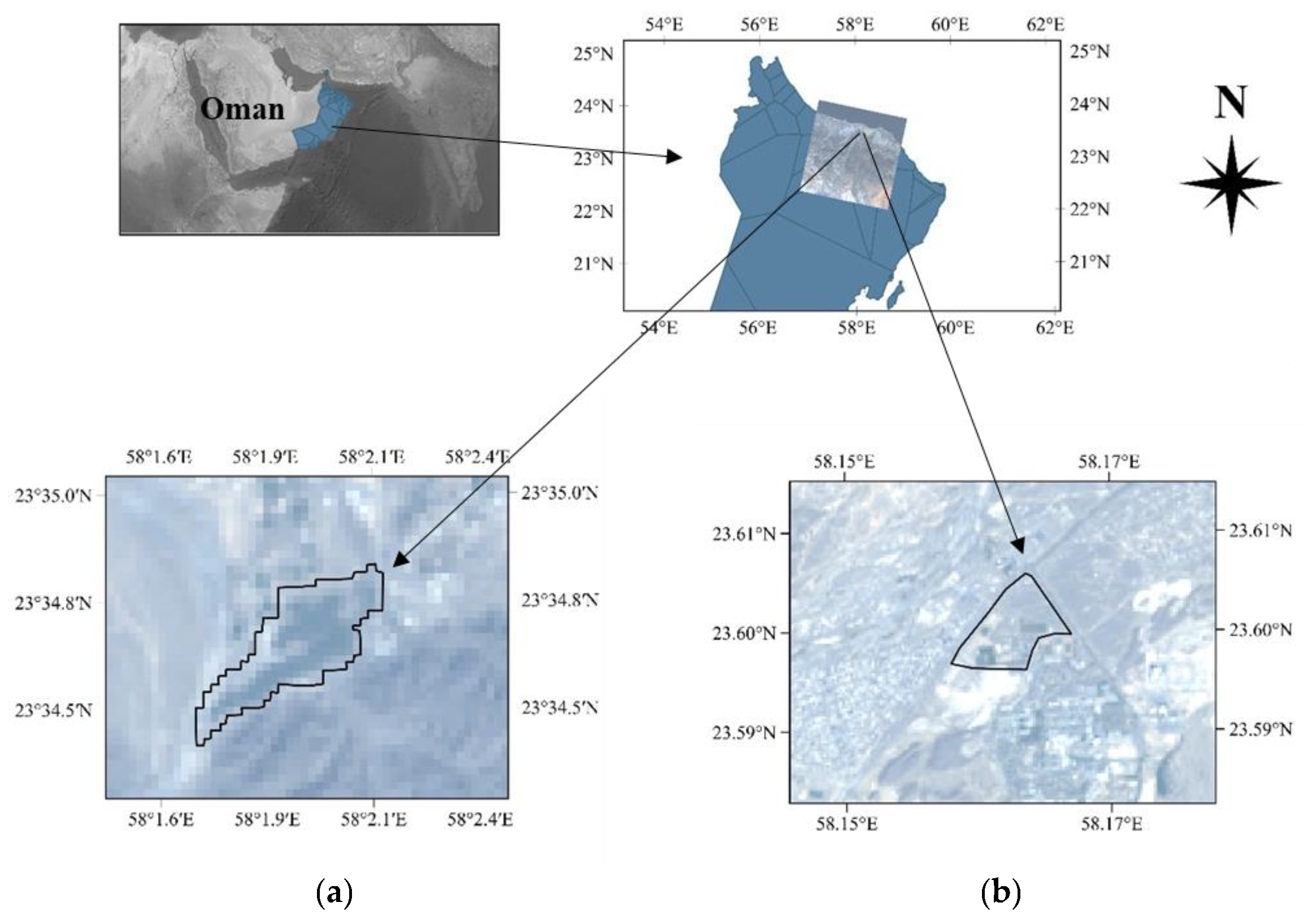
2.1. Study Area

Two experiment sites were selected for this study. The first site, with an area of 10 hectares, was a farm in the village of Halban (with latitude 23.57722° N and longitude 58.0322° E) in South Al-Batinah Governorate, Oman, located 45 km west of Muscat city. While the second site, with an area of 96 hectares, is located in the agricultural experiment station (AES) at Sultan Qaboos University (latitude 23.59861° N and longitude 58.16425°E). The ETa on Halban and the AES farm was observed for the complete year of 2015 and 2020, respectively. Both sites share the same climate, which can be categorized as hot and hyper-arid as the amount of average rainfall does not exceed 100 mm/year. The maximum temperature was recorded as 45.3 °C in the summer season. The temperature did not drop below 20 °C in extreme winter season. The selected farms were cultivated with date palm trees. A true colour composite image of bands 2, 3, and 4 of the study area is shown in Figure 1.

2.2. Satellite Imagery

All available images taken by the Landsat-OLI/TIRS during 2015 and 2020, with a total of 25 images, were used in this study. Acquisition dates Landsat-OLI/TIRS imagery is listed in

Table 1. Acquisition dates of Landsat-8 (OLI/TIRS) imagery (UTM-40N) used in the study area at Path “158” and Row “44” with a cloud coverage of less than 10%.

Acquisition Time		06:34:26.99 (GMT)	Temporal Resolution		16-Days
No	Julian Day	Date	No	Julian Day	Date
1	15	15 January 2015	14	61	1 March 2020
2	47	16 February 2015	15	93	2 April 2020
3	111	21 April 2015	16	109	18 April 2020
4	159	8 June 2015	17	125	4 May 2020
5	175	24 June 2015	18	157	5 June 2020
6	191	10 July 2015	19	173	21 June 2020
7	223	11 August 2015	20	189	7 July 2020
8	239	27 August 2015	21	237	24 August 2020
9	255	12 September 2015	22	253	9 September 2020
10	271	28 September 2015	23	269	25 September 2020
11	287	14 October 2020	24	285	11 October 2020
12	29	29 January 2020	25	317	12 November 2020
13	45	14 February 2020

. Digital numbers were first converted to radiance and then converted into reflectance values using header files for selected bands [41]. The digital elevation model (DEM) Version 2, with a spatial resolution of 1 arc-second (30 m), was used as an input for the surface elevation. The TIRS bands (100 m) were resampled to 30 m using the resampling techniques in ERDAS imagine v14.0 and using the nearest neighbor interpolation method. More information regarding the preprocessing and imagery used in this study can be found in [38].

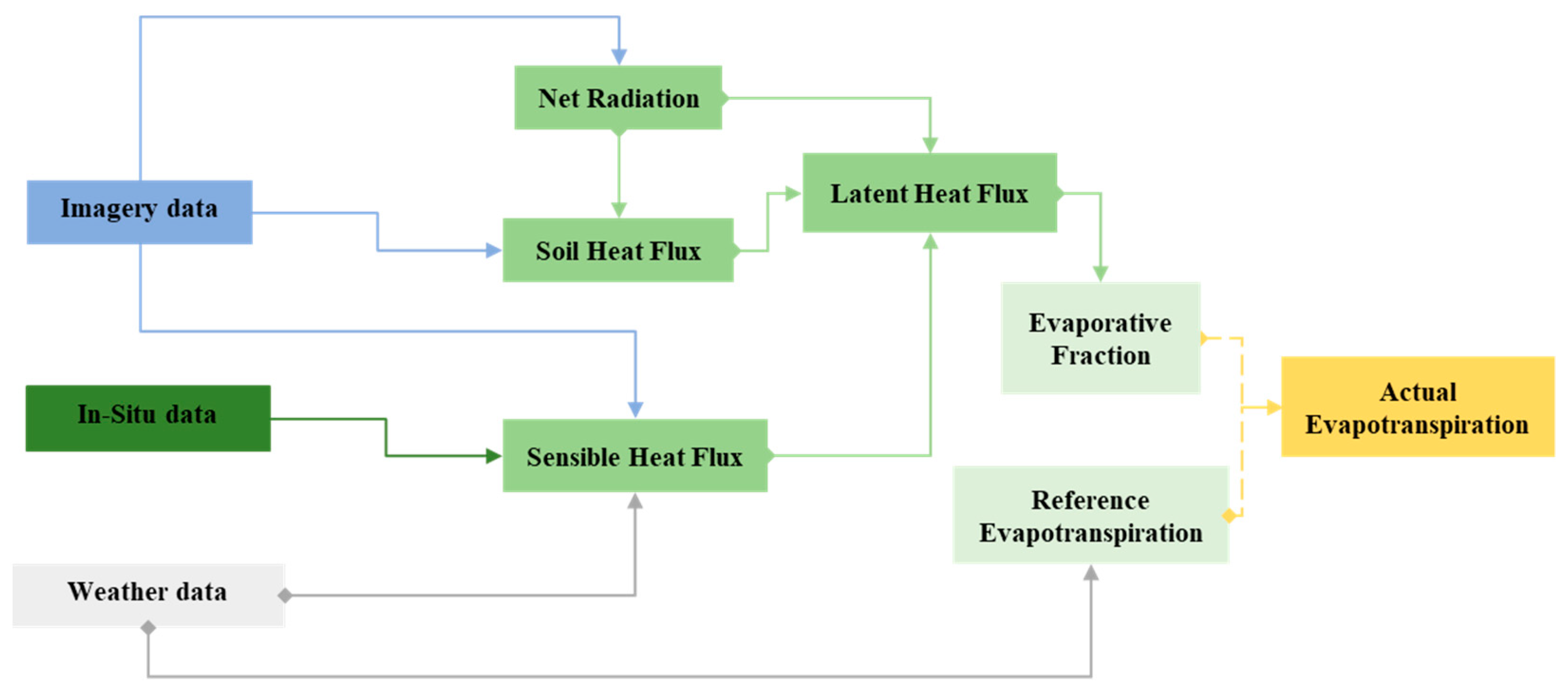
2.3. Satellite-Based Water and Energy Balance Model for the Arid Region to Determine Evapotranspiration (SMARET) Model Development

The satellite-based water and energy balance model for the arid aegion to determine evapotranspiration (SMARET) is based on the same concept of energy balance components used by SEBAL [22] and METRIC [11] to estimate ETa as residual energy. However, the SMARET model is a multi-level one-source model that estimates ETa as latent heat flux (LE) over the hot and hyper-arid region, as described in the following paragraphs and illustrated in Figure 2.

The latent heat flux (LE) is calculated using the following equation:

$$LE=Rn-G – H$$

(1)

where $Rn$ is the instantaneous net radiation (W m⁻²), $G$ is soil heat flux (W m⁻²), and $H$ is sensible heat flux (W m⁻²).

$$Rn={\mathrm{R}}^{\downarrow }-{\mathrm{R}}^{\uparrow }$$

(2)

where ${\mathrm{R}}^{\downarrow }$ is instantaneous net incoming radiation (W m⁻²) and ${\mathrm{R}}^{\uparrow }$ is the amount of instantaneous net outgoing radiation (W m⁻²). ${\mathrm{R}}^{\downarrow }$ is the total amount of incoming instantaneous net radiation that is received by the earth’s surface from solar radiation. On the other hand, ${\mathrm{R}}^{\uparrow }$ is the net amount of outgoing radiation that is reflected/emitted by the earth’s surface into the atmosphere. The amount of both, ${\mathrm{R}}^{\downarrow }$ and ${\mathrm{R}}^{\uparrow }$ are greatly affected by the amount and type of land cover on the earth’s surface and clouds. Therefore, SMARET was developed to suit cloud-free multispectral and thermal satellite imagery. Values of ${\mathrm{R}}^{\downarrow }$ were calculated from the installed weather station. However, ${\mathrm{R}}^{\downarrow }$ is spatially calculated on each pixel using the zenith angle as suggested by [22].

The required factors and their sources to feed them as inputs for SMARET are listed in

Table 2. Required input factors and their sources for the SMARET model.

Annotation	Factor	Source	Units
A	Albedo	Multispectral imagery (Bands 2–7)	(-)
NDVI	Normalized difference vegetation indices	Multispectral imagery (Bands 3 and 4)	(-)
LST	Land surface temperature	Thermal imagery (band 10–11)	(°K)
Rn	Net radiation	Multispectral and thermal imagery (bands 2–7, 10, and 11)	(Wm−2)
G	Soil heat flux	Multispectral and thermal imagery (bands 2–7, 10, and 11)	(Wm−2)
H	Sensible heat flux	Multispectral and thermal imagery (bands 2–7, 10, and 11), in situ data	(Wm−2)
ρair	Air density	Scaler input	(Kg m−3)
Cp	Specific heat of air at constant pressure	Scaler input	(J kg−1 K−1)
$R_{ah}$	Aerodynamic resistance to heat and air transport	Weather data	(s m−1)
${\mathrm{z}}_{0\mathrm{m}}$	Surface roughness length	Height of canopy, NDVI	(m)
U*	Friction velocity	Wind profile	(m s−1)
$d_o$	Zero-plane displacement	Mean height of the canopy	(m)
${\mathrm{z}}_{\mathrm{oh}}$	Roughness length for Heat	Wind profile	(m)
L	Monin–Obukhove length	Weather data imagery	(m)
${\tau }_{sw}$	Factor affecting atmospheric transmittance in air	Elevation of the study area	(m)

.

The SMARET model estimates soil heat flux (G) using an empirical relation between albedo (α), land surface temperature (LST), and the normalized difference vegetation indices (NDVI) following [25].

$$G=\frac{1}{\alpha }\left(Rn\times \mathrm{LST}\right)(0.0038\alpha +0.0074{\alpha }^2)\left(1-{\mathrm{NDVI}}^4\right)$$

(3)

Sensible heat flux (H) is a function of the temperature gradient, surface roughness, and wind speed and is thus difficult to compute due to the interrelationship of temperature gradient and surface roughness. The classical expression for H is given by [42]:

$$H=\frac{P_{air}\times C_p\times \left(dT\right)}{R_{ah}}$$

(4)

where H is sensible heat flux in W m⁻², Cp is air specific heat at constant pressure in J Kg⁻¹ K⁻¹, ${\rho }_{air}$ is atmospheric air density in Kg m⁻³, and $R_{ah}$ is the aerodynamic resistance to heat transport (s m⁻¹). dT is the temperature difference between air temperature and close-to-surface temperature.

SMARET is different from its predecessors such as SEBAL [22], S-SEBI [32], SEBAL-A [28], and METRIC [11] models in the estimation of dT values. In the SEBAL and METRIC models, dT values at each pixel are estimated using the inverse calibration technique. The SEBAL, SEBAL-A, and METRIC models select two extreme conditions in the study area: hot and cold pixels that act as an extreme boundary condition. However, the selection of these extreme conditions is very difficult [40] and needs expert hands. SMARET assumes that the heat transfer from the air to the plant is carried around the plant area. Hence, total plant height is considered in the SMARET model. Moreover, SMARET uses the soil and plant surface temperature to include more advection, a feature which was missing in the SEBAL model.

SMARET uses an innovative approach to estimate dT. The presence of CO₂, NO₂, O₃, and water content affects the accuracy of LST using thermal infrared sensors [43]. Ref. [44] stated that an accurate LST estimation is largely influenced by the difference between canopy emitted temperatures and the ground. According to [45], LST values usually represent only sunlit areas in the low vegetative area. On the other hand, LST values from the highly vegetated area are more accurately recorded from green leaves. According to [46], LST values affect the lower atmosphere and temperature difference between the canopy and the soil under it. Hence, the correct estimation of the temperature difference between the soil surface and plant surface at a reference height is difficult to obtain using satellite imagery on non-homogeneous surfaces. To minimize this difficulty in estimating the dT value, three scenarios (a, b, and c) were used to calculate dT values. In scenario (a), dT values were calculated as a temperature difference between the foliage surface temperature (Tfh, K) and the air temperate (Ta, K). In scenario (b), the difference between Tfh and soil surface (Ts, K) was considered. In scenario (c), the difference between Ts and Ta was considered. The three different temperature heights used in the three scenarios are shown in Figure 3.

The values of Ts were measured using 5TE sensors (model: 5TE, Meter Group, Washington, DC, USA), and the values of Tfh were obtained from satellite imagery. On the other hand, Ta was obtained from a VP4 sensor that was included in the weather station (model: TAHMO, Decagon Devices Inc., Washington, DC, USA), installed in the field. The installed weather station also included the following sensors: DS-2 decagon sonic anemometer to measure wind speed and direction; REC-1 rain gauge sensor to measure precipitation; VP4 sensor to measure, in addition to air temperature, the relative humidity; and pyranometer sensor to measure solar radiation.

SMARET hypothesizes that the first few centimeters of topsoil are very important for transfer from soil to air and can be affected greatly by the vegetation height or density. The SMARET model is different from its predecessors, SEBAL, SEBAL-A, and METRIC, as it does not require any extreme boundary conditions (hot and cold pixels) as these extreme conditions needed pixels based on accurate in situ information regarding crop and soil factors [40].

After the calculation of dT, the next step in SMARET was to calculate aerodynamic resistance to heat transport (R_ah). From Equation (4), it was not possible to estimate H with an unknown factor R_ah. Hence, an iteration process was initiated to correctly estimate R_ah values using correction factors at a given dT value. This process was started by considering an ideal condition where the lower boundary layer does not have an effect on wind speed, H, and R_ah on heat transport values using Equation (5).

$$R_{ah}=\frac{\ln \left(\frac{z_1}{z_2}\right)}{{\mathrm{U}}^{*} K}$$

(5)

where, $R_{ah}$ is aerodynamic resistance to heat transport (s m⁻¹), U* is the frictional velocity (m s⁻¹), ${\mathrm{z}}_{0\mathrm{m}}$ is defined by [9] as aero-dynamical roughness length for momentum transport (m) as formulated in Equation (6).

$${\mathrm{z}}_{0\mathrm{m}}=0.1\times Hc$$

(6)

According to [19], the reference site friction velocity U* can be calculated using Equation (7).

$${\mathrm{U}}^{*}=\frac{{\mathrm{U}}_{\mathrm{z}}\times 0.41}{\ln \left(\frac{\mathrm{z}}{{\mathrm{z}}_{0\mathrm{m}}}\right)}$$

(7)

U* is friction velocity for the reference site in m s⁻¹, ${\mathrm{z}}_{0\mathrm{m}}$ is surface roughness length in meters, and U_z is wind speed from the weather station (m s⁻¹).

In the next step, the iteration process was carried out to compensate for the effect of heat transport between two heights, Z₁ and Z₂. U* and R_ah values are corrected for the heat transport between two heights using Equations (8) and (9).

$${\mathrm{U}}^{*}=\frac{{\mathrm{U}}_{\mathrm{z}}\times 0.41}{\ln \left(\frac{z_r-d_o}{{\mathrm{z}}_{0\mathrm{m}}}\right)+{ \mathsf{\Psi }}_{m\left(z\right)}\left(\frac{z_r-d_o}{\mathrm{L}}\right) }$$

(8)

$$r_{ah}=\frac{\ln \left(\frac{z_0-d_o}{{\mathrm{z}}_{0\mathrm{m}}}\right)-{\mathsf{\Psi }}_h\left[\ln \left(\frac{{\mathrm{z}}_{0\mathrm{m}}}{{\mathrm{z}}_{\mathrm{oh}}}\right)\right]+\ln \left(\frac{{\mathrm{z}}_{0\mathrm{m}}}{{\mathrm{z}}_{\mathrm{oh}}}\right)}{{\mathrm{U}}^{*}\times 0.41}$$

(9)

where, ${\mathsf{\Psi }}_h$ is the stability factor that is formulated in Equations (12)–(14). By using Equation (10), the value of the Monin–Obukhov length (L) determines the new constant to be added to compensate for the stability due to height and wind. Hence, the iteration process begins using Equations (10)–(13):

$$L=-\frac{\rho c_p{\mathrm{U}}_{\ast }^3\mathrm{LST}}{KgH}$$

(10)

where ρ is the density of air (kg m⁻²), cp is the air specific heat as 1004 J kg⁻¹ K⁻¹, U* is the friction velocity (m s⁻¹), LST is the land surface temperature in K, and g is the gravitational constant (9.81 ms⁻²). For unstable conditions (L less than zero), the formulation by [47,48] was used as explained:

$${\mathsf{\Psi }}_{h\left(z\right)}=2\ln \left(\frac{1+X_{\left(z\right)}{}^2}{2}\right)$$

(11)

where:

$${\mathrm{X}}_{\left(z\right)}={\left(1-16\frac{z}{L}\right)}^{0.25}$$

(12)

For stable conditions (L greater than zero), the formulas are:

$${\mathsf{\Psi }}_{h\left(z\right)}=-5 \left(\frac{z}{L}\right)$$

(13)

For neutral conditions (L equals zero), stability values are kept at zero. On the other hand, if the value of L equals or is greater than zero, then values of ${\mathrm{X}}_{\left(z2\right)}$ and ${\mathrm{X}}_{\left(z1\right)}$ have no meaning, and their values are set to one. The new value of corrected L determines the corrected values of R_ah called R_ah1. The new value of R_ah1 was then used in Equation (9), and new values of H were calculated. Hence, the process continued until the values of Rah and H were stable.

LE is the available amount of energy flux that is used by the plant/atmosphere or both to convert water into vapors to be released in the form of evaporation and transpiration or both (ETa). To detect ETa, the correct estimation of Rn, G, and H is required. These values are estimated at an instantaneous level using satellite imagery. According to [9], daily estimates of ETa are important compared to instantaneous estimates of ETa at the time of satellite overpasses. Hence, to obtain the daily cumulative LE, different fractions/factors have been previously used. The FAO Penman–Monteith (PM) equation uses crop factor (Kc) to estimate ETa using metrological datasets [10]. The Kc value is dependent to crop type, age, growth, and vegetation growth stage [11]. According to [32], S-SEBI uses surface reflectance and surface temperature to estimate evaporative fraction as it assumes atmospheric conditions to be kept the same across the whole area. The METRIC model uses instantaneous reference evaporative fraction (ErF) to extrapolate ET_inst to ETa. However, the value of ErF is assumed to be constant to estimate ETa on a daily basis for fully vegetated crops. According to [9], ErF can decrease in the afternoon, especially in areas with less available water due to the less advection process. Hence, evaporative fraction (EF), used by the SEBAL model, can be used to better extrapolate LE to ETa values. SMARET uses [25]’s approach to use $\mathrm{EF}$ as an estimate of Rn, G, and H, formulated in Equation (14). While EF act as:

$$\mathrm{EF}=\frac{LE}{Rn-G}=\frac{Rn-G-H}{Rn-G}$$

(14)

While:

$$ETa=E{T}_{r24}\times \mathrm{EF}$$

(15)

Here, ET_r24 is the 24 h daily cumulative hourly-based-reference ET (mm d⁻¹) for an alfalfa crop using the standardized ASCE (American Society of Civil Engineers) Penman–Monteith equation for the day of satellite image acquisition. For the estimation of ET_r24, parameters from the weather station were used, and the ET for the reference alfalfa crop was estimated. Then, each hourly value of ET_r was added for the estimation of ET_r24.

2.4. SMARET Model Validation and Evaluation

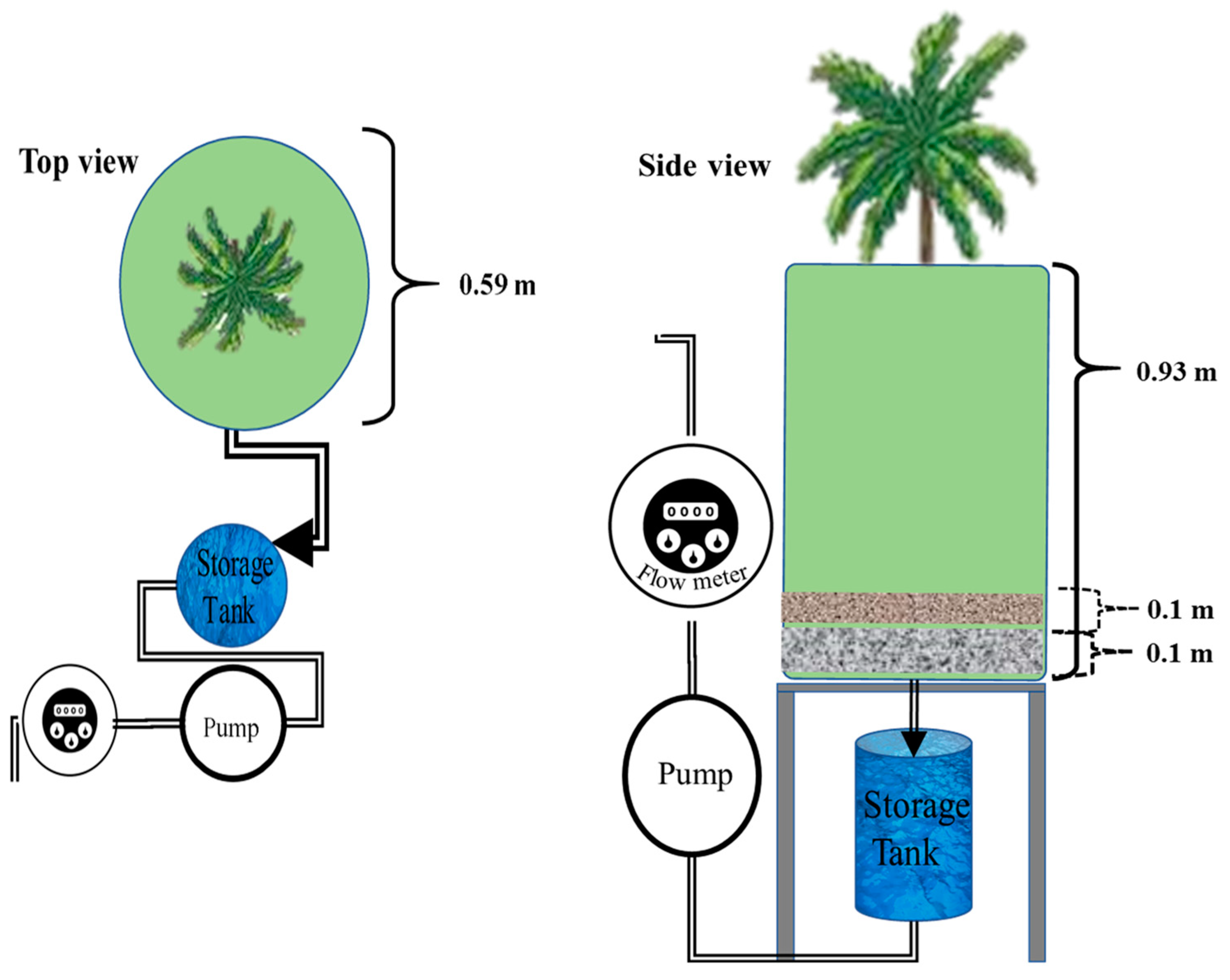
Direct evapotranspiration measurements, using drainage-type lysimeters, as described in the following paragraphs, were taken to validate the SMARET model. The model was also evaluated against the predecessor’s models, including SEBAL, METRIC, and PM.

2.4.1. Lysimeters

To validate the SMARET model, two drainage-type lysimeters (200 L capacity each) were installed on the date palm tree in the agricultural experiment station (AES), Sultan Qaboos University, Oman. Date palm trees aged 3–4 years were planted and irrigated by a controlled drip irrigation system used at the AES farm. Figure 4 shows the design layout of the installed lysimeter. Ref. [49] suggested a drainage system to prevent waterlogging in the lysimeter. On each lysimeter, two drains with mesh (1-inch diameter each) were drilled and connected to a storage tank with a storage capacity of 25 L. Each drain was covered with the 10 cm layer of gravel having a size of 1.5 to 2 cm, followed by a 10 cm layer of fine gravel (size of 0.2 cm). Each lysimeter was refilled with the excavated soil from the same site. Irrigation was applied manually on the surface. Before the plantation of the date palm tree in the lysimeter, a 15 cm layer of soil was first refilled in the lysimeter to keep maximum roots in contact with soil. As suggested by [50], each lysimeter was installed equally to the ground surface to minimize the effect of wind and temperature with the container wall. The soil in the AES was sandy stone with a bulk density of 1.49 g cm⁻³. The soil electrical conductivity (EC) was 0.18 mS cm⁻¹ with a moisture content of 0.12 m³ m⁻³.

2.4.2. Surface Energy Balance for Land (SEBAL)

The surface energy balance for land (SEBAL) model is a physically-based surface energy balance model that was considered as a pioneer to estimate surface parameterization based on vertical temperature difference [22]. The SEBAL model was applied in the study area to estimate actual ETa (mm d⁻¹) as described by [22] using Landsat-8 OLI/TIRS images.

$$E{T}_a=E{T}_{po{t}_{24}}\times (Rn-G-H)/(Rn-G)$$

(16)

where, $E{T}_{po{t}_{24}}$ is the 24 h potential evapotranspiration in mm d⁻¹ esteemed by using daily net radiation $\left(R{n}_{24}\right)$ (W m⁻²) following [19]:

$$E{T}_{po{t}_{24}}=\frac{R{n}_{24}}{\lambda \times {\rho }_{\omega }}\times 864\times {10}^5$$

(17)

2.4.3. Mapping Evapotranspiration at High Resolution with Internalized Calibration (METRIC)

METRIC (mapping evapotranspiration at high resolution with internalized calibration), the successor of the SEBAL model, has been widely used as a remote sensing-based model that estimates ETa as a residual of the surface energy balance equation by satellite imagery and metrological data using Equation (18).

$$E{T}_{inst}=3600\times \frac{Rn-G-H}{\lambda \times {\rho }_{\omega }}$$

(18)

METRIC is modified from SEBAL as it uses weather-based reference ET to calibrate ETa from the satellite. In METRIC, daily ETa is calculated over the area as:

$$ETa=E{T}_{r24}\times \frac{E{T}_{inst}}{E{T}_r}$$

(19)

ET_r24 is the 24 h daily cumulative of hourly-based-reference ET (mm d⁻¹) for an alfalfa crop using the standardized ASCE (American Society of Civil Engineers) Penman–Monteith equation for the day of satellite image acquisition. For the estimation of ET_r24, parameters from the weather station were used, and the ET for the reference alfalfa crop was estimated. Then each hourly value of ETr was added for the estimation of ET_r24. More details on SEBAL and METRIC can be found in [11,22,51].

2.4.4. Modified Penman–Monteith (PM) Model

Modified Penman–Monteith (PM) model was used based on [10] by which the PM model is used to measure ETa (Equation (20)) using reference evapotranspiration (ET_r) incorporation with a dimensionless crop factor (Kc).

$$ETa=E{T}_r\times \mathrm{Kc}$$

(20)

ETr is calculated by using Equation (21) which was used to estimate ET_r for different times and space while details on Kc can be found in [10]. The needed weather parameters for the model (e.g., temperature, wind speed, solar radiation, precipitation, humidity, and sunshine hours) were obtained from the installed weather station at the study site.

$$E{T}_r=\frac{0.408∆\left(R_n-G\right)+\gamma \frac{900}{T+273}{u}_2\left(e_s-e_a\right)}{∆+\gamma \left(1+0.34u_2\right)}$$

(21)

where, ET_r is the reference evapotranspiration rate from a wide, uniform surface of dense 0.5 m tall alfalfa crop, (mm d⁻¹), Rn is net radiation at the crop surface (MJ m⁻² d⁻¹), G is soil heat flux density in (MJ m⁻² d⁻¹), u₂ is the wind speed at 2 m height (m s⁻¹), es is saturation vapor pressure [kPa], e_a is expressing actual vapor pressure (k Pa), e_s − e_a is saturation vapor pressure deficit (kPa), ∆ is denotes slope vapor pressure curve (kPa °C⁻¹), and γ is psychrometric constant (kPa °C⁻¹).

3. Results and Discussions

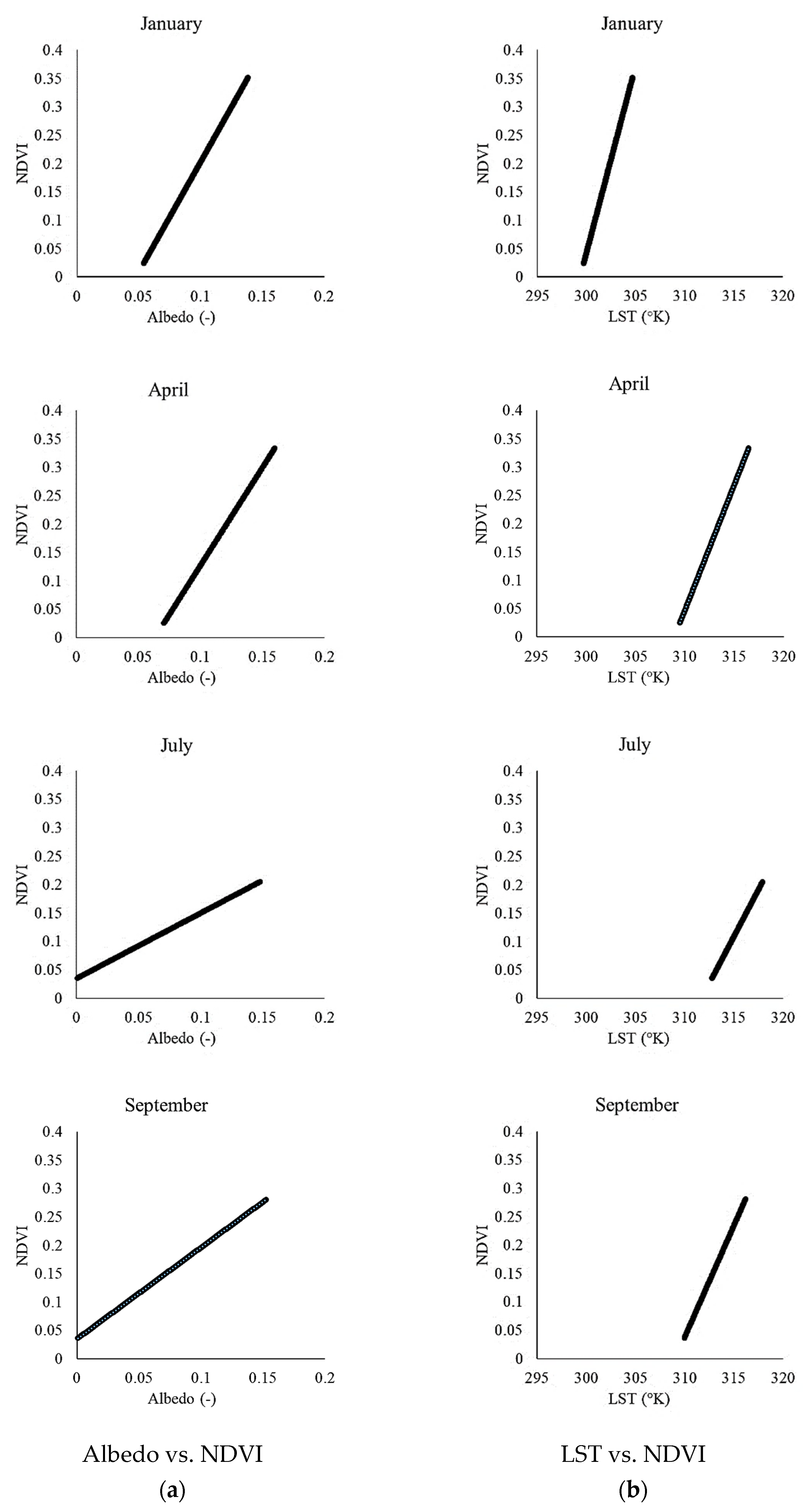
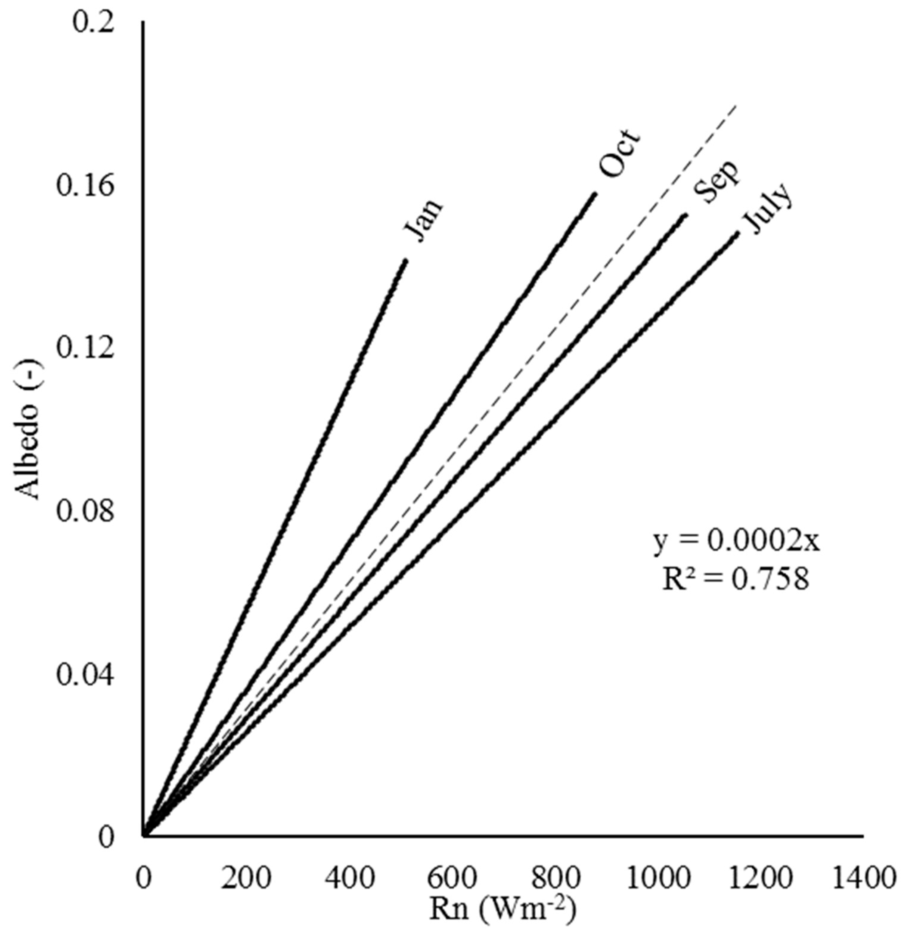
3.1. Albedo (α) vs. Normalized Difference Vegetation Indices (NDVI)

A relationship between albedo (α) and the normalized difference vegetation indices (NDVI) was observed, as shown in Figure 5a. The study concluded that there was a strong positive correlation between α and NDVI, especially in the fruit development period (January–April). On the other hand, in the harvesting period (June–July), the slope between α and NDVI was less steep as compared to the fruit development period. One of the reasons might be the decrease in NDVI values as fruit from the trees was harvested in the summer season. Pruning (removal of old/damaged leaves) was carried out, which led to the low value of NDVI in the post-harvesting season (September–November) that caused a gentle slope in the albedo–NDVI relationship.

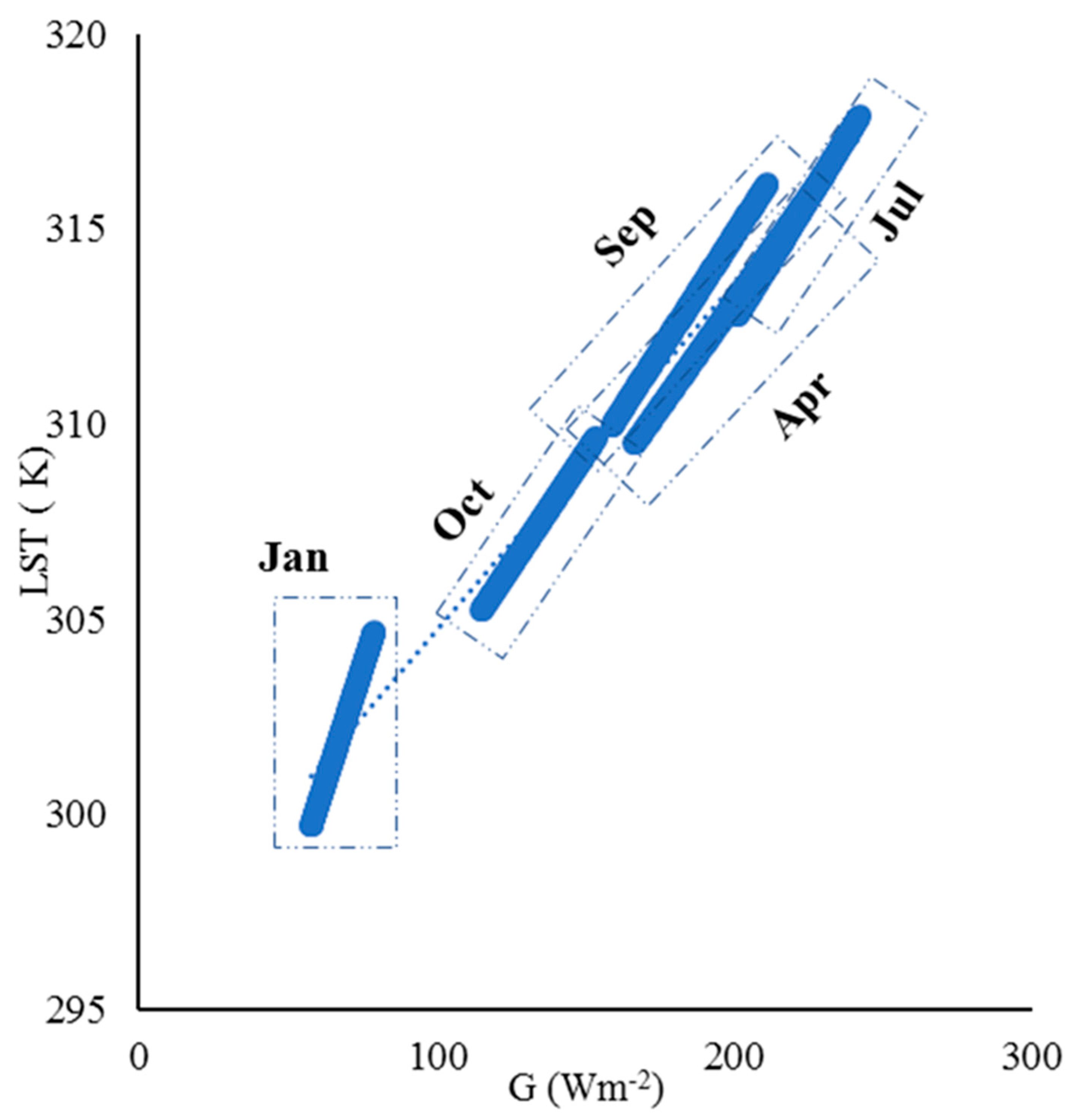
3.2. Land Surface Temperature (LST) vs. Normalized Difference Vegetation Indices (NDVI)

NDVI is a factor for the proportion of vegetation on the surface, while land surface temperature (LST) is the temperature of the surface of the obstacle (crops, trees, buildings, and soil). The study resulted in a correlation (Figure 5b) that was strong with positive steep slopes in the fruit development season and post-harvesting season when the values of NDVI were higher. As the climate got hotter, an increase in the LST value was observed as the fruit was harvested from the trees, which also led to a decrease in the NDVI value, thus causing a relatively less steep slope. Therefore, this study resulted in the values of NDVI having a direct effect on LST, especially in hot conditions.

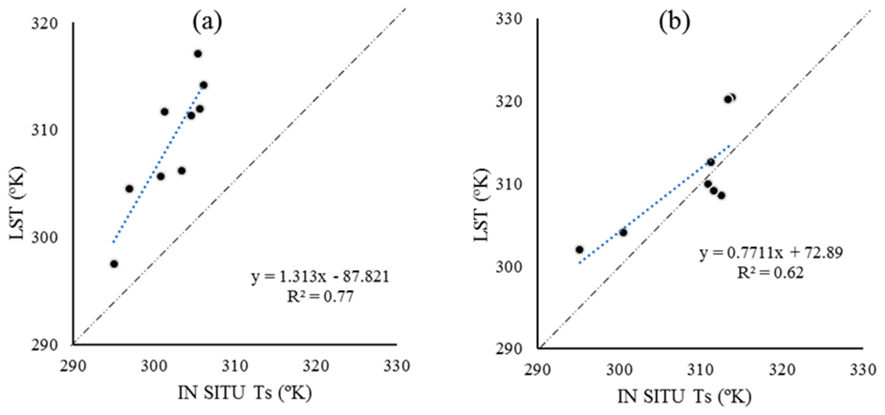
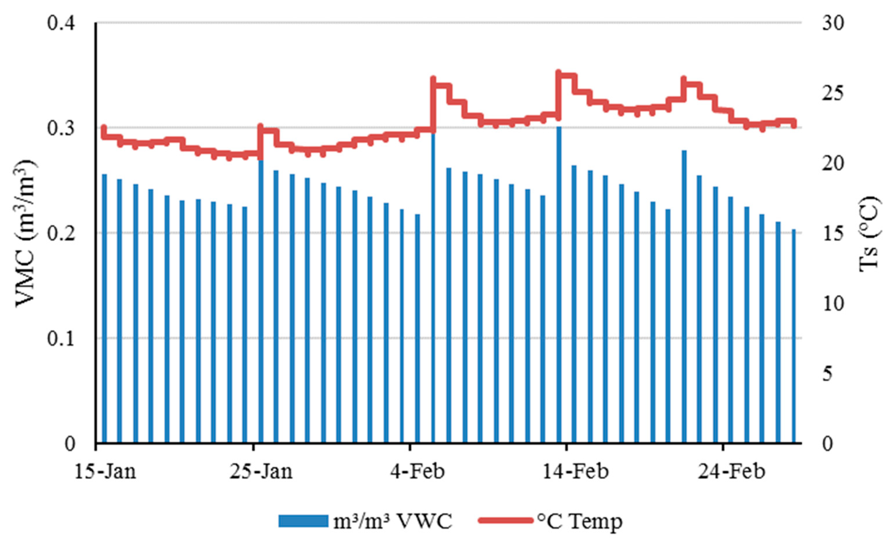
3.3. Land Surface Temperature (LST) vs. In Situ Soil Temperature (Ts)

A strong relationship was found between LST and in situ soil temperate (Ts), as shown in Figure 6. The Ts (°K) was recorded using 5TE sensors installed in the soil at two locations. Figure 6a was recorded in the Halban area, which was covered with date palm trees having higher NDVI values. On the other hand, Figure 6b show the relationship on a relatively low vegetated area. Figure 6 show that the value of Ts was lower in an area with high vegetation, which is caused by the shading effect, as more than 70% of the soil in that area was under constant shade. On the other hand, the slope between LST and Ts was less steep in the less vegetated area, causing a relatively less strong relationship between the LST and Ts values. The studyconcluded that at the time of irrigation, the temperature of soil increased and then started to decrease once the moisture content of soil reduced, as shown in Figure 7.

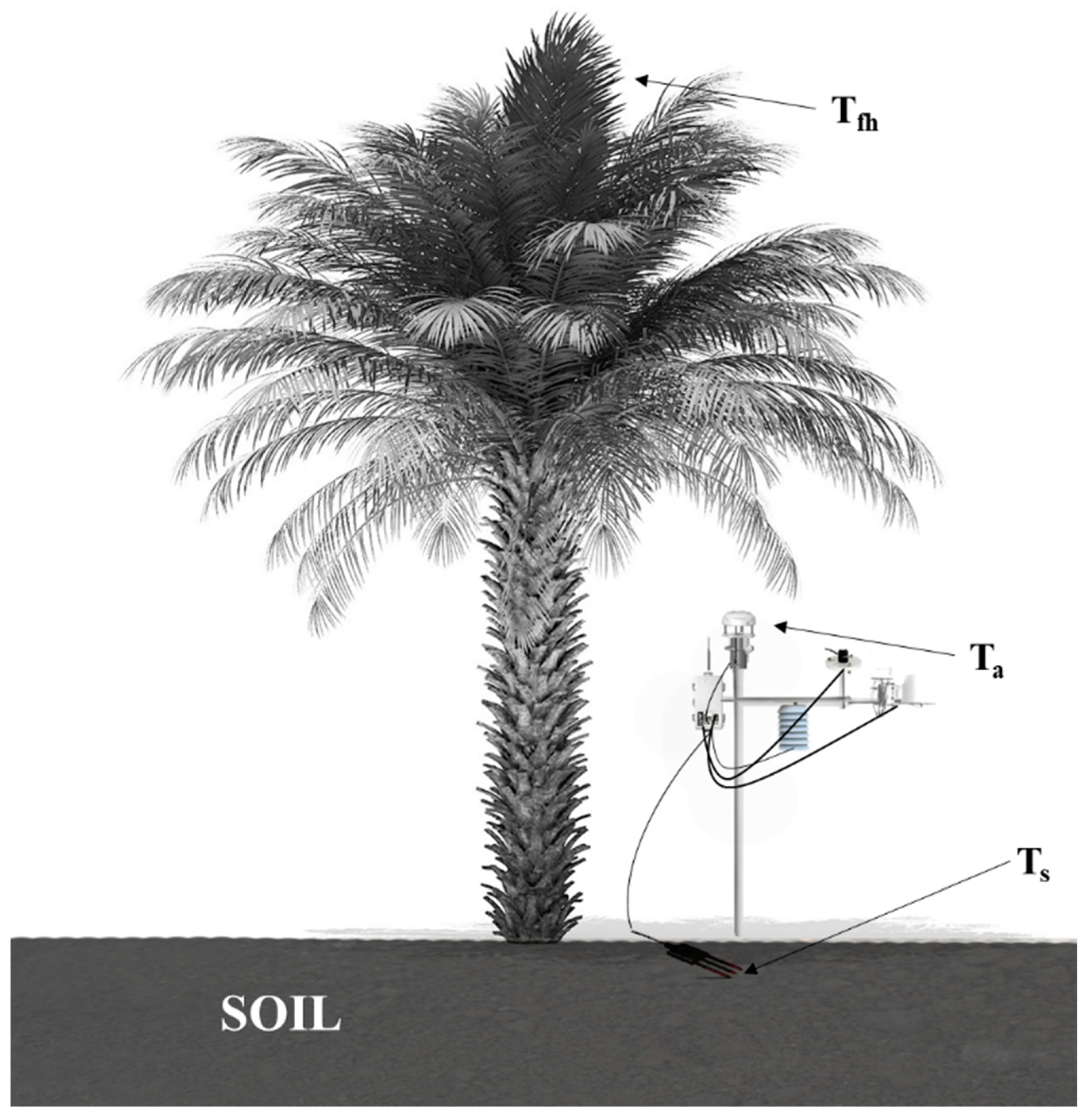
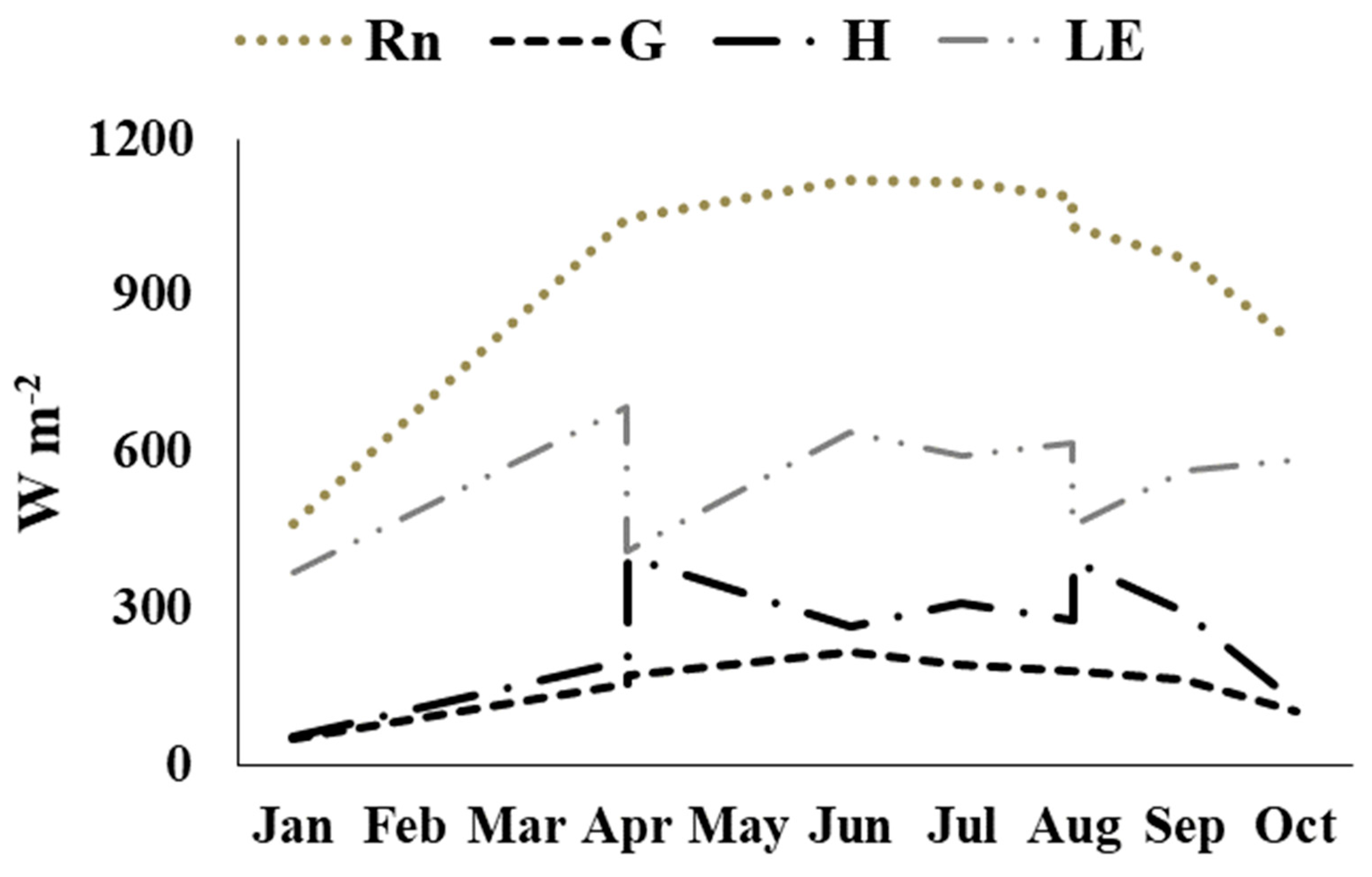
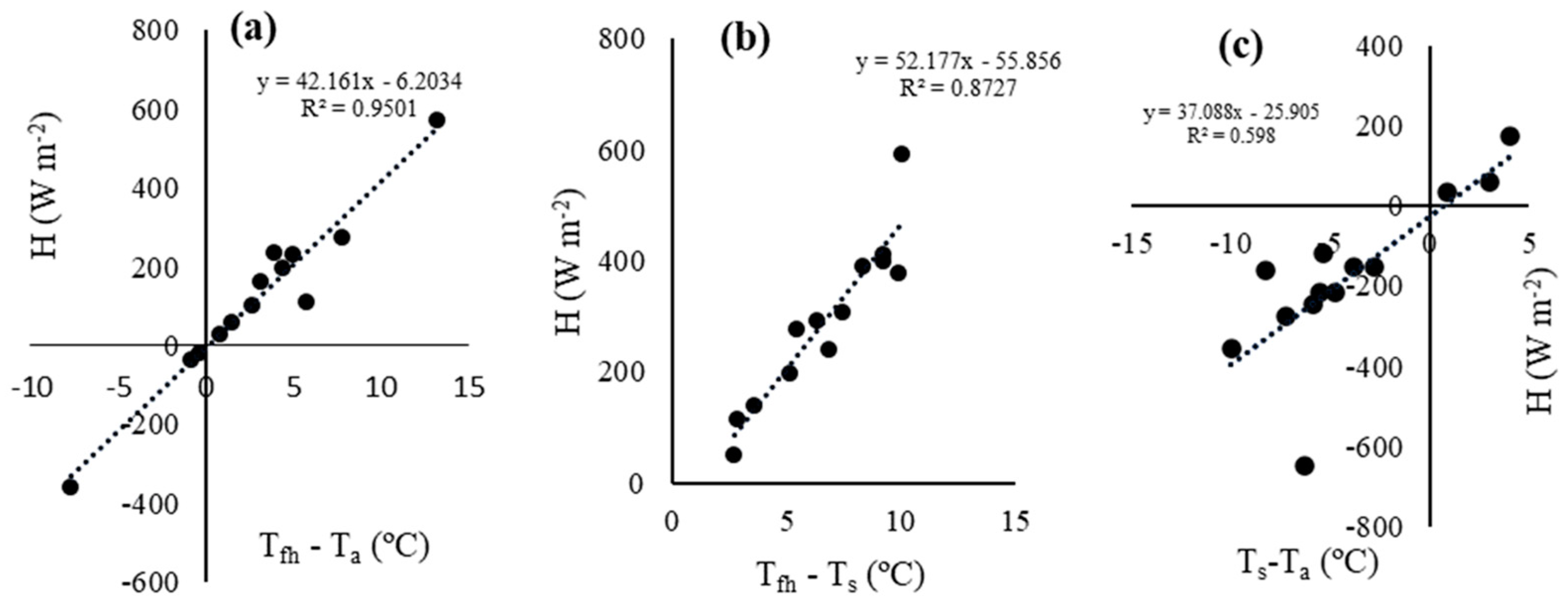
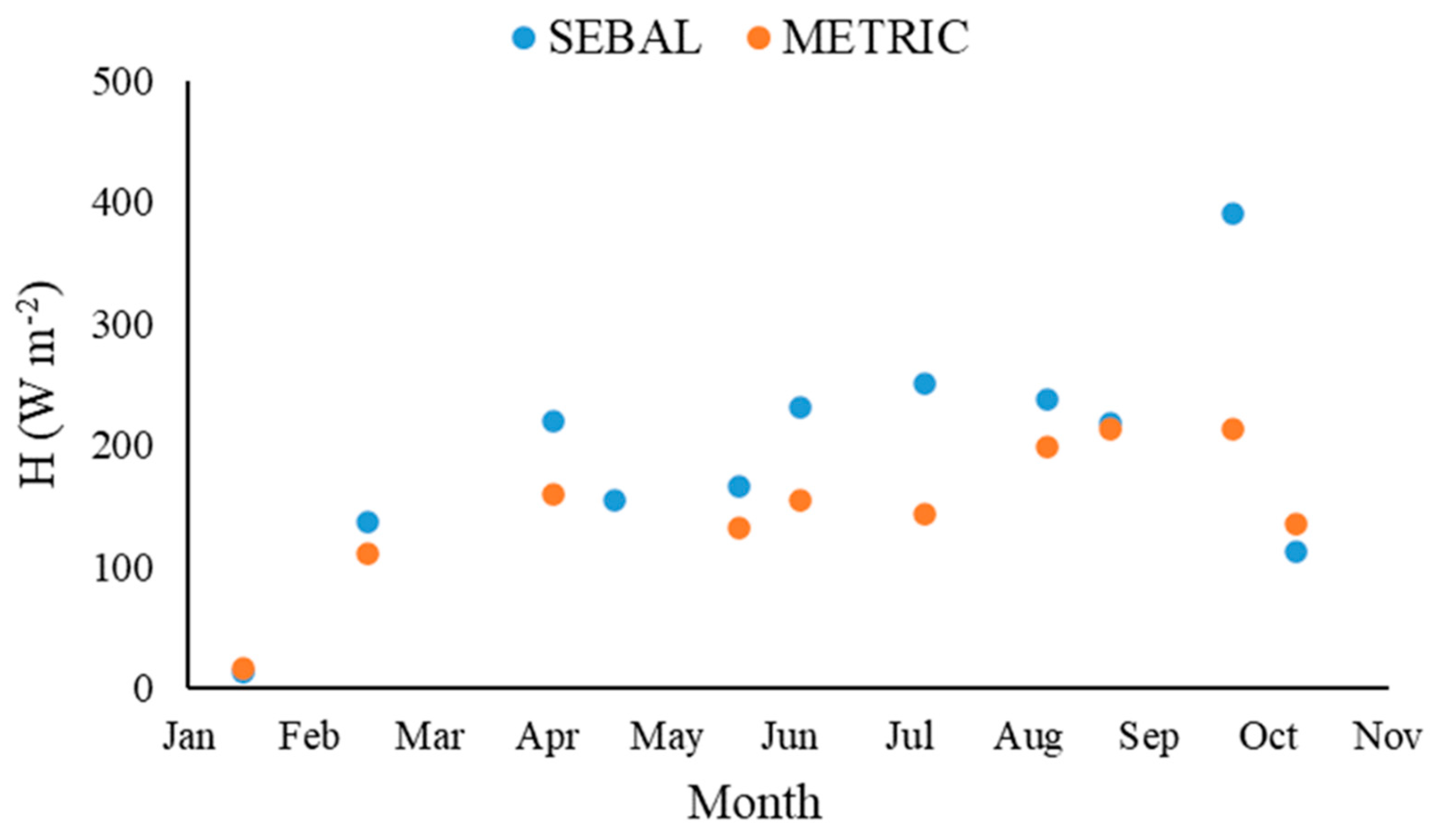
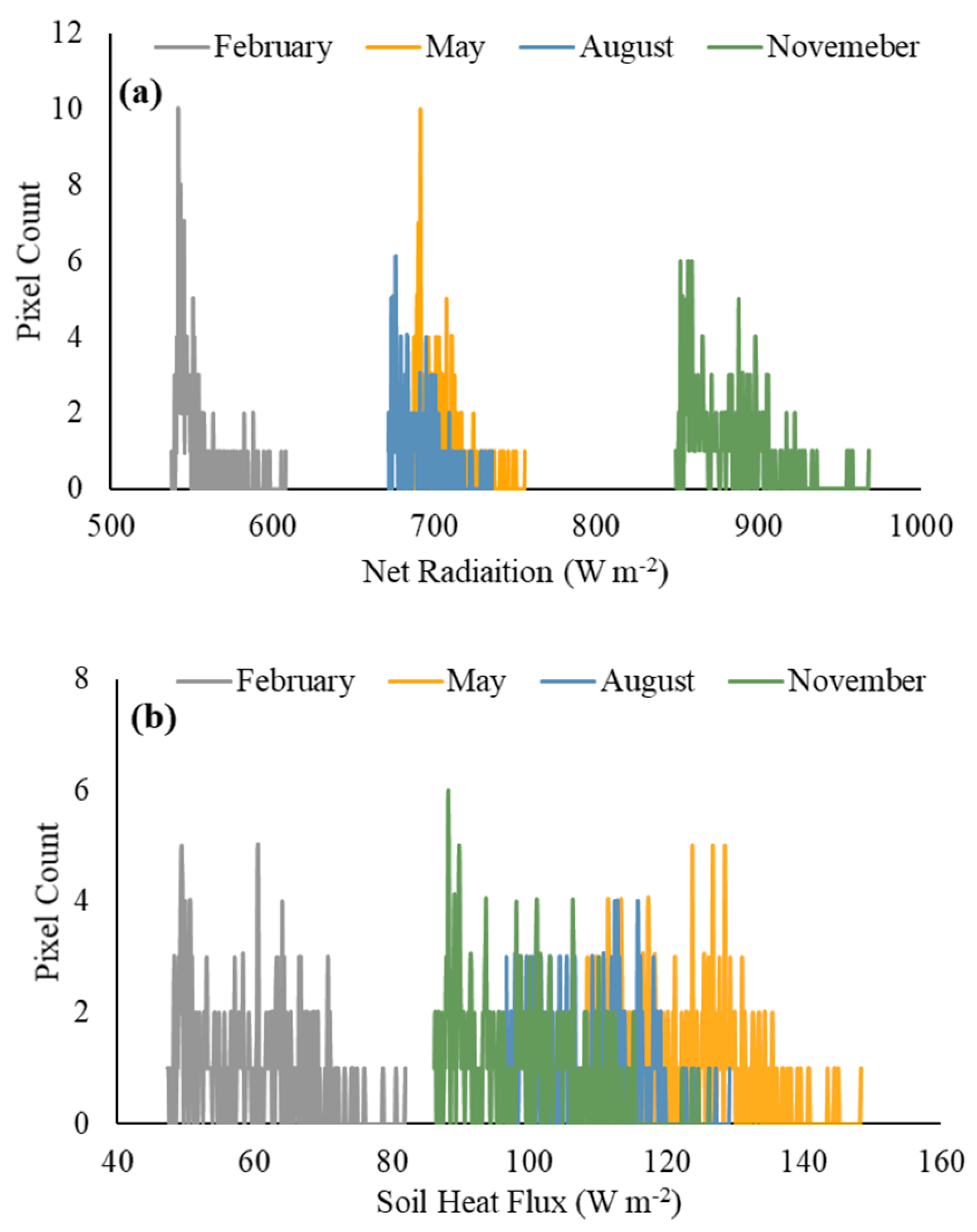
3.4. The Magnitude of Energy Fluxes

Energy balance components (Rn, G, and H) were calculated as shown in Figure 1. Figure 8 show the temporal changes in the energy fluxes in the year 2015 at the Halban site. The results have shown that the values of Rn were increasing as the weather got hotter. The maximum amount of Rn was observed from July to August, from the lowest of 1029 W m⁻² in August to the highest value of 1109 W m⁻² in June. The same trend was observed with the values of G as the values of G were recorded with the lowest value of 48.568 W m⁻² in January and the highest value of 275 W m⁻² in June (Figure 8). On the other hand, the SMARET model resulted in a difference of 16 W m⁻² between Halban and the SQU site in the year 2020, as the value of G recorded in SQU was 147 W m⁻² in June 2020 while Halban recorded 131 W m⁻². The difference between the two values was caused by the difference in NDVI and LST values.

Figure 9 show a correlation between the α and Rn values for a complete year. In the early stage of fruit development, the value of α was observed to be higher because of the highest reflection of solar radiation from the leaf. Hence a very little amount of heat was absorbed by the leaves. This scenario led to a low value of Rn in the early fruit development stage. On the other hand, July is the peak time of harvesting fruit. Hence, the available radiation for the photosynthesis process was higher, which led to a positive correlation (with a less steep slope) between α and Rn in harvesting time. The post-harvest season (September and October) showed a much steeper α vs. Rn slope. The reason might be that in the tall crops, such as date palm, Rn values decreased as more solar outgoing radiations were reflected from the leaves. As shown in Figure 5a, α is also affected by the NDVI values, which might be one of the reasons for the increase in slope in the post-harvest season.

Figure 10 show a strong correlation between LST and G for the study area. Results have shown that overall, LST and G were showing an increasing trend for the date palm. In the early pre-fruit development, the slope of LST was steep with a value of 0.235, as the LST was recorded with the lowest value in the study area with the lowest values of G. The study also concluded that the value of the slope decreases from the highest value to the lowest value of 0.115 in October (post-harvest) as the LST values increases. Being a hot and hyper-arid area, the value of G was recorded with a highest value of 9.5% of Rn in fruit development season, which is under the limit of 10% as stated by [52,53,54,55,56]. The lowest value of G/Rn (5%) was observed in September as the LST values were started to decrease, as shown in Figure 6.

After the successful estimation of Rn and G, H was estimated using Equation (3) after examining the three scenarios of determining dT as described in the methodology section and illustrated in Figure 3. The dT values for each scenario are presented in

Table 3. Values of temperature difference dT (°C) observed in study area using three different scenarios.

Month	dT = Tfh − Ta	dT = Tfh − Ts	dT = Ts − Ta
Jan	5.76	2.7	3
Feb	7.74	6.8	0.9
Apr	−0.42	5.1	−5.5
Jun	2.67	9.9	−7.2
Jul	1.48	7.4	−5.9
Aug	3.11	5.4	−5.4
Sep	−7.72	6.3	−6.3
Oct	−0.81	2.8	−2.8
SD	4.91	2.61	4.25

.

The values of dT from each scenario were used in the iteration process to estimate the correct values of Rah in Equation (3). Statistics show that there was a linear relationship between the dT and H value as the regression coefficient (R²) was higher than 0.85 in scenarios “a” and “b”. Results have also shown that as the values of dT increase or decrease from a threshold value, the values of H goes below zero, allowing the SMARET model to apply a limit on dT values. Each scenario with the estimated value of H is shown in Figure 11.

The application of limits to dT values was assigned based on the values of H. Scenario (a) and (c) were neglected as dT values ranged below zero, which led to values of H below zero. The study concluded that the negative values of H and Rah cannot be achieved even in ideal conditions. These results were strengthened by the values of H estimated by both SEBAL and METRIC models in the same study area. The values of H estimated using SEBAL, and METRIC models have been shown in Figure 12.

Another reason to select scenario “b” was the values of deviation of means. Even though scenario “a” shows the highest value of R², the standard deviation of mean (SD) values of scenario “b” were minimal (2.6 °C) as compared to the other. Hence scenario “b” was selected as the best for the SMARET model.

The estimated values of H from the three scenarios were used to estimate ETa values. Results have shown that Scenario “b” has shown the lowest amount of error as compared to in-field values. ETa values of the SMARET model were compared with the ETa values from an experiment conducted by [38]. Results have shown that scenario “b” used in the SMARET model was in a good correlation (R² = 0.66) with the ETa values recorded using sap flow meter (Figure 13).

Figure 14 strengthens the selection of scenario (b) in the SMARET model as scenario (c) overestimated the values of ETa as compared with scenarios (a) and (b). Scenario (a) resulted in the highest ETa overestimation of 5 mm d⁻¹ by the SMARET model, but scenario (c) was on the top with the highest value of 8 mm d⁻¹. On the other hand, scenario (b) resulted in the highest overestimation of 1.7 mm d⁻¹. Moreover, scenarios (a) and (c) produce mean errors of 1.90 mm d⁻¹ and 3.94, respectively, while scenario (b) produces a mean error of 0.43 mm d⁻¹.

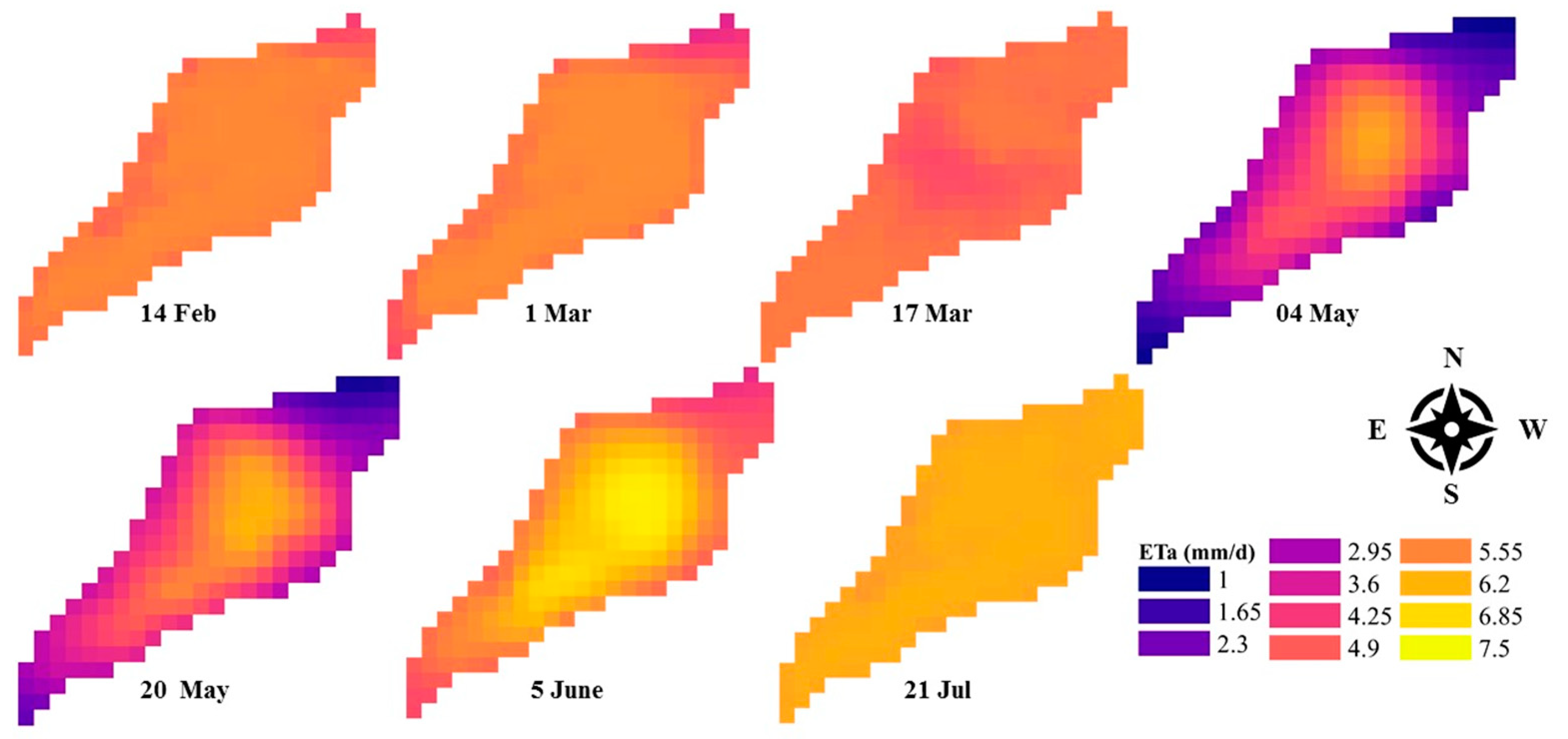
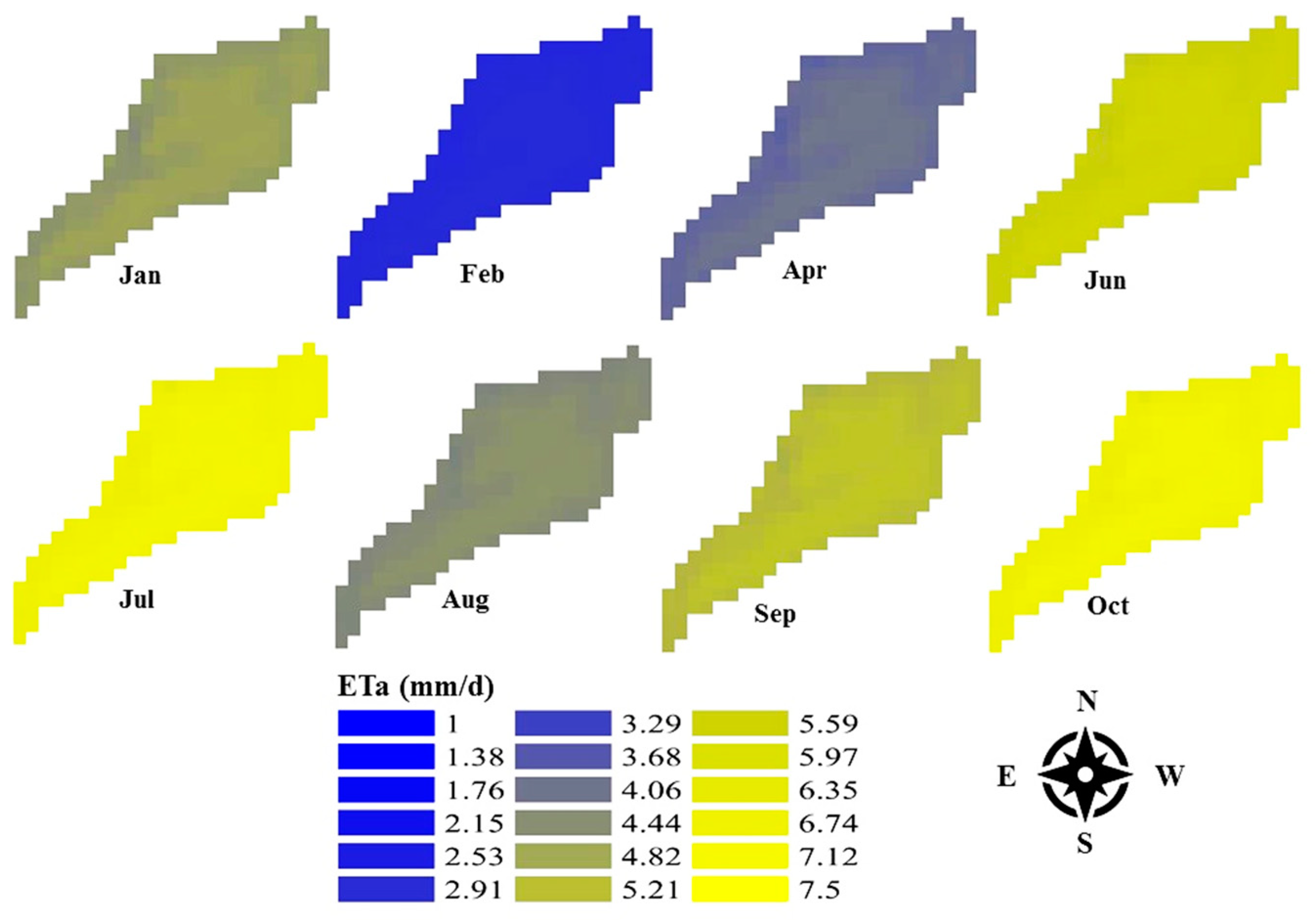
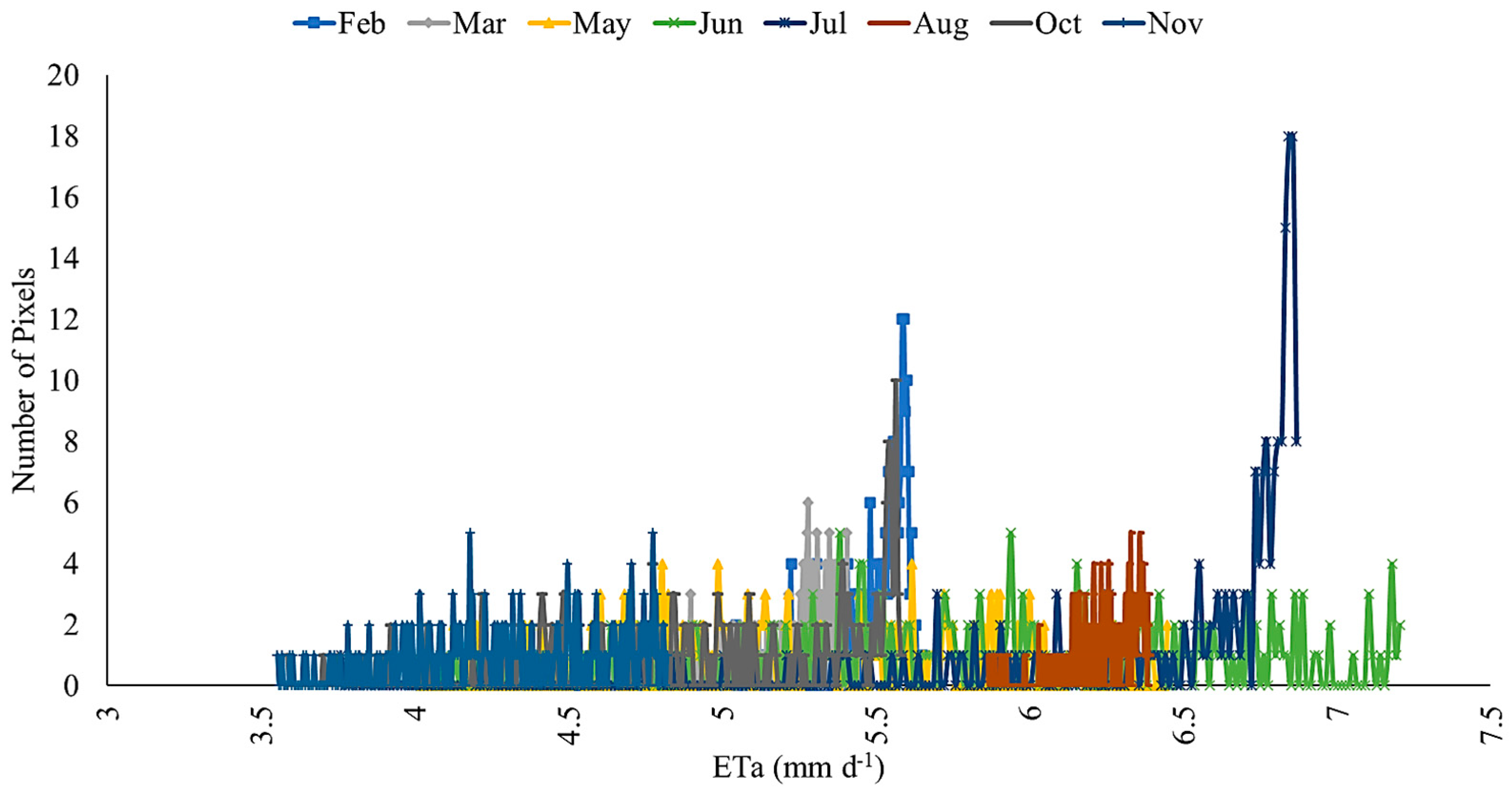
3.5. Magnitude of Actual Evapotraspiration (ETa)

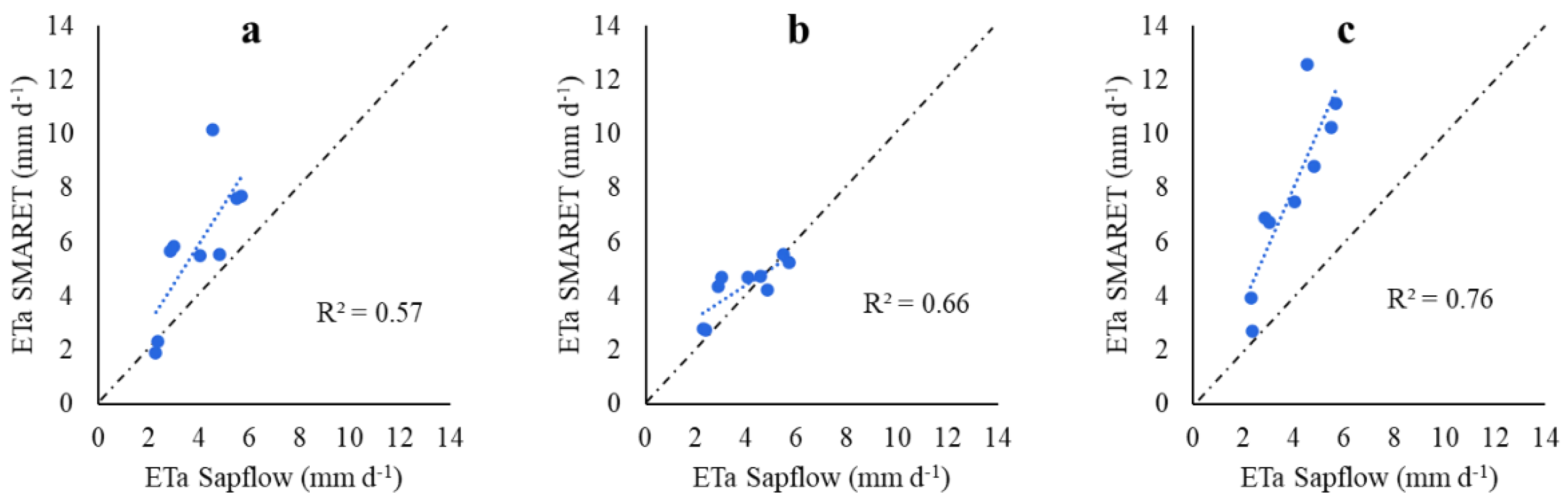
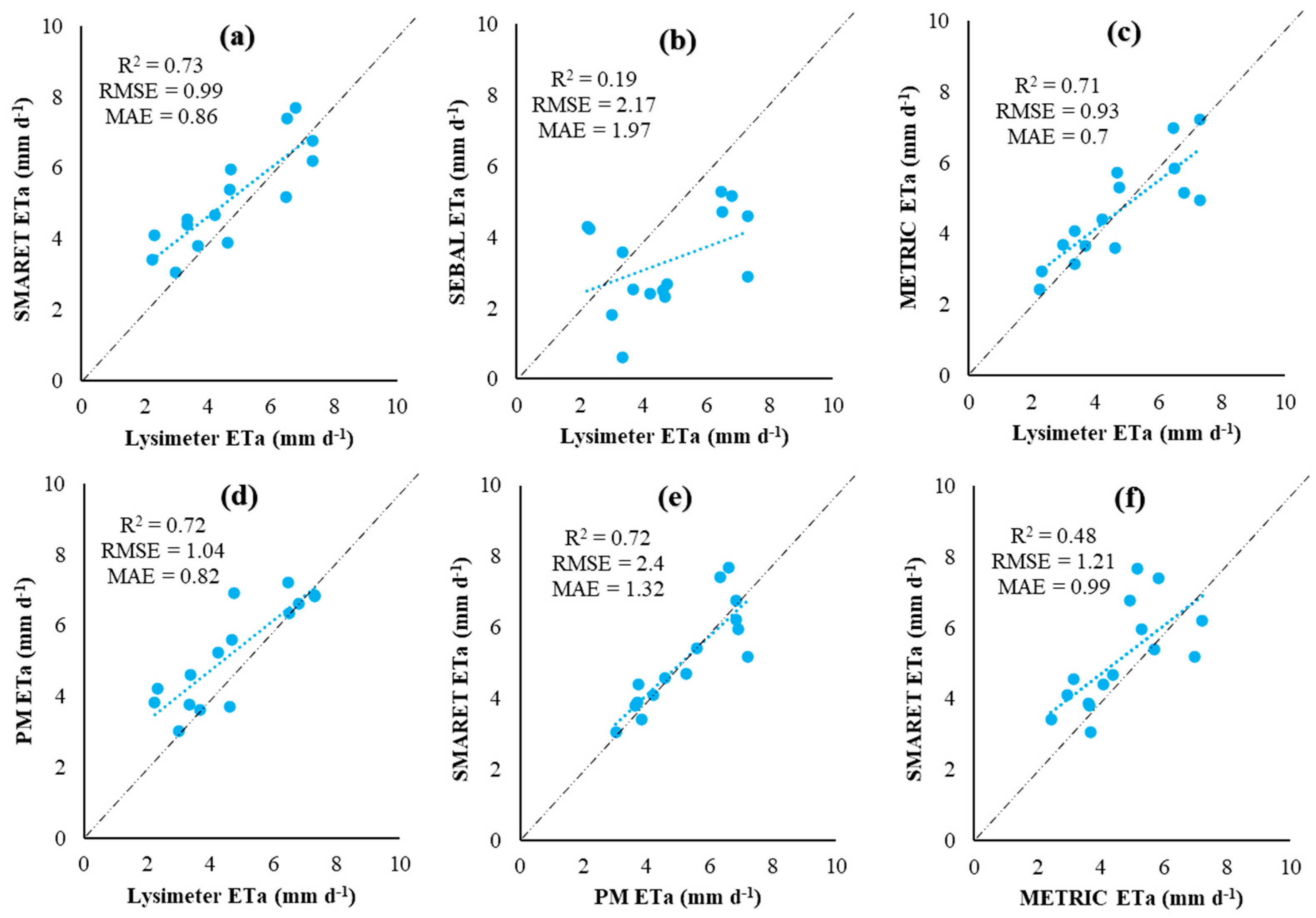
The SMARET model estimated ETa values for February with a maximum value of 2.7 mm d⁻¹ in 2015, while the value in Halban was 4.7 mm d⁻¹ in 2020. The spatial distribution of the SMARET model is shown in Figure 14 and Figure 15. This difference in ETa value is caused by the increase in the age of date palm. The same trend was observed in June for the Halban area. In 2015, ETa values were estimated over Halban area was 5.59 mm d⁻¹ which was increased to 6.3 mm d⁻¹.

Results have shown that the ETa values estimated with the SMARET model ranged from 0 to 8 mm d⁻¹ for the period. The study area observed that the ETa values in February ranged from 5 mm d⁻¹ to 5.7 mm d⁻¹ as the NDVI values showed a spatial distribution of vegetation over course of the study. The study area observed the highest value of NDVI in February as the LST values were less than 302 K. The study area resulted in a spatial variation of ETa values in May as the values ranged from 0 to 6 mm d⁻¹. Results have shown a narrow range of NDVI values in May from 0.02 to 0.35. This might lead to an average of 12 K increase in LST. Moreover, the values of G were also 100 Wm⁻² higher than in February. Although the LST values in August decreased to a maximum value of 306 K, there was no significant difference between the values of NDVI in May and August. The highest values of ETa in August might be due to the increase in the available amount of energy fluxes (Figure 16).

The results have shown that the highest values of Rn and G were observed in May as compared to August. The results have shown that both Rn and G values decreased in August as compared with the value of Rn and G in May. This could be due to the decrease in LST values in August. The highest values of Rn were observed in November, but the NDVI of the study area did not change significantly. The SMARET model resulted in a 25% and 33% increase of ETa in August as compared to May and February, respectively (Figure 17).

4. Validation

The SMARET model was also validated against the SEBAL, METRIC, and PM models, as well as with in situ measurement using lysimeter. SEBAL, METRIC, and PM models were applied to the AES site for the validation of the SMARET model. The difference of ETa values of SMARET was observed to be 0.2 mm d⁻¹, 2 mm d⁻¹, 0.6 mm d⁻¹, and 2.2 mm d⁻¹ with SEBAL, METRIC, PM, and lysimeter, respectively. It was observed that the models overestimated ETa in the fruit development stage as compared to lysimeter measurements. The overestimation of ETa values in the SMARET values continued in the fruit development stage in the mid of April until the temperature in April started to increase. It was observed that the SMARET model was underestimating ETa values in the pre-harvesting season. Validation results showed that the METRIC and PM models were overestimating ETa in the pre-harvesting season, and the difference reached maximum values of 2 mm d⁻¹ in the harvesting season. Validation results showed that the SMARET model and lysimeter were very close to each other in the post-harvesting season.

Figure 18 show the correlation between all the models and lysimeter. Figure 18a represent the correlation of ETa values by SMARET and lysimeter showing an acceptable correlation with the regression coefficient (R²) value of 0.73 as SMARET was overestimating in the early validation period. The PM method and lysimeter (Figure 18b) showed a good positive correlation in estimating ETa with an R² value of 0.83. Error in absolute mean was also less than 1 mm d⁻¹, but the PM model was overestimating ETa values in pre-harvesting season. Results showed that SEBAL did not show a good correlation (R² = 0.14) of ETa with lysimeter values with the highest value of mean absolute error.

5. Conclusions

Traditionally, the estimation of actual evapotranspiration (ETa), in the form of evaporation from soil and transpiration from the plant, was approximated using different in situ techniques such as PAN-measurements, sap flow, Bowen ratio, and the Eddy covariance system. However, these methods have high initial and maintenance costs with a low spatial resolution and can only be applied to small areas. On the other hand, ETa is considered an important component of the surface water budget monitored by satellite imagery. This study developed and tested a surface energy-balance satellite imagery model (SMARET) to estimate ETa for hot and hyper-arid regions. The newly developed model coupled the satellite imagery with in situ measurements from the field and validated the sap flow meter and lysimeter against in situ devices. The developed model was also evaluated against other existing models, including surface energy balance algorithm for land (SEBAL), mapping evapotranspiration at high resolution with internalized calibration (METRIC), and the Penman–Monteith (PM) method. The SMARET model provided a great variety of energy fluxes within the study area. Results have shown that the value of net radiations (Rn) and soil heat flux (G) decreased in August as compared with May due to decreased land surface temperature values. The SMARET model was validated against SEBAL, METRIC, PM, and lysimeter. The overall trend has shown that the ETa values estimated by the SMARET model were high but closer to the PM and lysimeter readings in the summer as compared to the SEBAL and METRIC models. The study resulted in a good correlation between SMARET (R² = 0.73), as well as PM model (R² = 0.72), and ETa values calculated from lysimeter. The SMARET model had a significant correlation (R² = 0.66) with the ETa values recorded using the sap flow meter. The strong relationship between SMARET, sap flow measurement, and lysimeter observation suggests that our model has the application capability in hot and hyper-arid regions. It is worth mentioning that, currently, SMARET is only valid for ETa estimation in hyper-arid regions using Landsat-8 imagery.

References

1. Brown, J.J.; Das, P.; Al-Saidi, M. Sustainable Agriculture in the Arabian/Persian Gulf Region Utilizing Marginal Water Resources: Making the Best of a Bad Situation. Sustainability 2018, 10, 1364. [Google Scholar] [CrossRef] [Green Version]
2. Dodds, P.E.; Barton, A.; Meyer, W.S. Review of Methods to Estimate Irrigated Reference Crop Evapotranspiration Across Aus-tralia; Technical Report 04/05; CRC for Irrigation Futures and CSIRO Land and Water: Adelaide, SA, Australia, 2005. [Google Scholar]
3. Li, Z.L.; Tang, R.; Wan, Z.; Bi, Y.; Zhou, C.; Tang, B.; Yan, G.; Zhang, X. A review of current methodologies for regional evapo-transpiration estimation from remotely sensed data. Sensors 2009, 9, 3801–3853. [Google Scholar] [CrossRef] [Green Version]
4. Zhang, K.; Ma, J.; Zhu, G.; Ma, T.; Han, T.; Feng, L.L. Parameter sensitivity analysis and optimization for a satellite-based evap-otranspiration model across multiple sites using Moderate Resolution Imaging Spectroradiometer and flux data. J. Geo-Phys. Res. Atmos. 2017, 122, 230–245. [Google Scholar] [CrossRef]
5. Zhang, K.; Kimball, J.S.; Running, S.W. A review of remote sensing based actual evapotranspiration estimation. Wiley Interdiscip. Rev. Water 2016, 3, 834–853. [Google Scholar] [CrossRef]
6. Eagleman, J.R. Pan evaporation, potential and actual evapotranspiration. J. Appl. Meteorol. Climatol. 1967, 6, 482–488. [Google Scholar] [CrossRef] [Green Version]
7. Sakuratani, T. A Heat Balance Method for Measuring Water Flux in the Stem of Intact Plants. J. Agric. Meteorol. 1981, 37, 9–17. [Google Scholar] [CrossRef]
8. Running, S.; Baldocchi, D.; Turner, D.; Gower, S.; Bakwin, P.; Hibbard, K. A Global Terrestrial Monitoring Network Integrating Tower Fluxes, Flask Sampling, Ecosystem Modeling and EOS Satellite Data. Remote Sens. Environ. 1999, 70, 108–127. [Google Scholar] [CrossRef]
9. Allen, R.; Irmak, A.; Trezza, R.; Hendrickx, J.M.H.; Bastiaanssen, W.; Kjaersgaard, J. Satellite-based ET estimation in agriculture using SEBAL and METRIC. Hydrol. Process. 2011, 25, 4011–4027. [Google Scholar] [CrossRef]
10. Allen, R.G.; Pereira, L.S.; Raes, D.; Smith, M. Crop Evapotranspiration—Guidelines for Computing Crop Water Requirements; FAO Irrigation and Drainage Paper 56; FAO: Rome, Italy, 1998; Volume 300, p. D05109. [Google Scholar]
11. Allen, R.G.; Walter, I.A.; Elliott, R.; Itenfisu, D.; Brown, P.; Jensen, M.E.; Mecham, B.; Howell, T.A.; Snyder, R.; Eching, S.; et al. Task Committee on Standardization of Reference Evapotranspiration. 2005. ASCE: Reston, VA, USA. Available online: https://epic.awi.de/id/eprint/42362/1/ascestzdetmain2005.pdf (accessed on 8 January 2018).
12. Seemann, S.W.; Li, J.; Menzel, W.P.; Gumley, L.E. Operational Retrieval of Atmospheric Temperature, Moisture, and Ozone from MODIS Infrared Radiances. J. Appl. Meteorol. 2003, 42, 1072–1091. [Google Scholar] [CrossRef]
13. Pereira, L.S.; Teodoro, P.R.; Rodrigues, P.N.; Teixeira, J.L. Irrigation scheduling simulation: The model ISAREG. In Tools for Drought Mitigation in Mediterranean Regions; Springer: Dordrecht, The Netherland, 2003; pp. 161–180. [Google Scholar]
14. Liu, Y.; Teixeira, J.; Zhang, H.; Pereira, L. Model validation and crop coefficients for irrigation scheduling in the North China plain. Agric. Water Manag. 1998, 36, 233–246. [Google Scholar] [CrossRef]
15. Idso, S.B.; Aase, J.K.; Jackson, R.D. Net radiation—Soil heat flux relations as influenced by soil water content variations. Boundary-Layer Meteorol. 1975, 9, 113–122. [Google Scholar] [CrossRef]
16. Jackson, R. Evaluating evapotranspiration at local and regional scales. Proc. IEEE 1985, 73, 1086–1096. [Google Scholar] [CrossRef]
17. Norman, J.M.; Kustas, W.P.; Humes, K.S. Source approach for estimating soil and vegetation energy fluxes in observations of directional radiometric surface temperature. Agric. For. Meteorol. 1995, 77, 263–293. [Google Scholar] [CrossRef]
18. Anderson, M.C.; Norman, J.M.; Mecikalski, J.R.; Otkin, J.A.; Kustas, W.P. A climatological study of evapotranspiration and moisture stress across the continental United States based on thermal remote sensing: 1. Model formulation. J. Geophys. Res. Space Phys. 2007, 112. [Google Scholar] [CrossRef]
19. Sun, Z.; Wang, Q.; Matsushita, B.; Fukushima, T.; Ouyang, Z.; Watanabe, M.; Gebremichael, M. Further evaluation of the Sim-ReSET model for ET estimation driven by only satellite inputs. Hydrol. Sci. J. 2013, 58, 994–1012. [Google Scholar] [CrossRef] [Green Version]
20. Irmak, A.; Kamble, B. Evapotranspiration data assimilation with genetic algorithms and SWAP model for on-demand irrigation. Irrig. Sci. 2009, 28, 101–112. [Google Scholar] [CrossRef]
21. Losgedaragh, S.Z.; Rahimzadegan, M. Evaluation of SEBS, SEBAL, and METRIC models in estimation of the evaporation from the freshwater lakes (Case study: Amirkabir dam, Iran). J. Hydrol. 2018, 561, 523–531. [Google Scholar] [CrossRef]
22. Bastiaanssen, W.; Menenti, M.; Feddes, R.; Holtslag, B. A remote sensing surface energy balance algorithm for land (SEBAL). 1. Formulation. J. Hydrol. 1998, 212-213, 198–212. [Google Scholar] [CrossRef]
23. Bastiaanssen, W.G.; Pelgrum, H.; Wang, J.; Ma, Y.; Moreno, J.F.; Roerink, G.J.; Van der Wal, T. A remote sensing surface energy balance algorithm for land (SEBAL).: Part 2: Validation. J. Hydrol. 1998, 212, 213–229. [Google Scholar] [CrossRef]
24. Al Zayed, I.S.; Elagib, N.A.; Ribbe, L.; Heinrich, J. Satellite-based evapotranspiration over Gezira Irrigation Scheme, Sudan: A comparative study. Agric. Water Manag. 2016, 177, 66–76. [Google Scholar] [CrossRef]
25. Bastiaanssen, W. SEBAL-based sensible and latent heat fluxes in the irrigated Gediz Basin, Turkey. J. Hydrol. 2000, 229, 87–100. [Google Scholar] [CrossRef]
26. Sun, H.; Yang, Y.; Wu, R. Improving estimation of cropland evapotranspiration by the Bayesian model averaging method with surface energy balance models. Atmosphere 2019, 10, 188. [Google Scholar] [CrossRef] [Green Version]
27. Mkhwanazi, M.; Chávez, J.L.; Andales, A.A. SEBAL-A: A Remote Sensing ET Algorithm that Accounts for Advection with Limited Data. Part I: Development and Validation. Remote Sens. 2015, 7, 15046–15067. [Google Scholar] [CrossRef] [Green Version]
28. Allen, R.G.; Burnett, B.; Kramber, W.; Huntington, J.; Kjaersgaard, J.; Kilic, A.; Kelly, C.; Trezza, R. Automated Calibration of the METRIC-Landsat Evapotranspiration Process. JAWRA J. Am. Water Resour. Assoc. 2013, 49, 563–576. [Google Scholar] [CrossRef]
29. French, A.N.; Hunsaker, D.J.; Thorp, K.R. Remote sensing of evapotranspiration over cotton using the TSEB and METRIC energy balance models. Remote Sens. Environ. 2015, 158, 281–294. [Google Scholar] [CrossRef]
30. Kjaersgaard, J.; Allen, R.; Irmak, A. Improved methods for estimating monthly and growing season ET using METRIC applied to moderate resolution satellite imagery. Hydrol. Process. 2011, 25, 4028–4036. [Google Scholar] [CrossRef]
31. Trezza, R. Evapotranspiration from a remote sensing model for water management in an irrigation system in Venezuela. Interciencia 2006, 31, 417–423. [Google Scholar]
32. Roerink, G.; Su, Z.; Menenti, M. S-SEBI: A simple remote sensing algorithm to estimate the surface energy balance. Phys. Chem. Earth Part B Hydrol. Ocean. Atmos. 2000, 25, 147–157. [Google Scholar] [CrossRef]
33. Bhattarai, N.; Shaw, S.B.; Quackenbush, L.J.; Im, J.; Niraula, R. Evaluating five remote sensing based single-source surface energy balance models for estimating daily evapotranspiration in a humid subtropical climate. Int. J. Appl. Earth Obs. 2016, 49, 75–86. [Google Scholar] [CrossRef]
34. Rocha, N.; Käfer, P.; Skokovic, D.; Veeck, G.; Diaz, L.; Kaiser, E.; Carvalho, C.; Cruz, R.; Sobrino, J.; Roberti, D.; et al. The Influence of Land Surface Temperature in Evapotranspiration Estimated by the S-SEBI Model. Atmosphere 2020, 11, 1059. [Google Scholar] [CrossRef]
35. Galleguillos, M.; Jacob, F.; Prevot, L.; Lagacherie, P.; Liang, S. Mapping Daily Evapotranspiration Over a Mediterranean Vineyard Watershed. IEEE Geosci. Remote Sens. Lett. 2010, 8, 168–172. [Google Scholar] [CrossRef]
36. Kumar, U.; Sahoo, B.; Chatterjee, C.; Raghuwanshi, N.S. Evaluation of Simplified Surface Energy Balance Index (S-SEBI) Method for Estimating Actual Evapotranspiration in Kangsabati Reservoir Command Using Landsat 8 Imagery. J. Indian Soc. Remote Sens. 2020, 48, 1421–1432. [Google Scholar] [CrossRef]
37. dos Santos, C.A.C.; Mariano, D.A.; Nascimento, F.D.C.A.D.; Dantas, F.R.D.C.; de Oliveira, G.; Silva, M.T.; da Silva, L.L.; da Silva, B.B.; Bezerra, B.; Safa, B.; et al. Spatio-temporal patterns of energy exchange and evapotranspiration during an intense drought for drylands in Brazil. Int. J. Appl. Earth Obs. Geoinf. 2019, 85, 101982. [Google Scholar] [CrossRef]
38. Madugundu, R.; Al-Gaadi, K.A.; Tola, E.; Hassaballa, A.A.; Patil, V.C. Performance of the METRIC model in estimating evapotranspiration fluxes over an irrigated field in Saudi Arabia using Landsat-8 images. Hydrol. Earth Syst. Sci. 2017, 21, 6135–6151. [Google Scholar] [CrossRef] [Green Version]
39. Nisa, Z.; Khan, M.; Govind, A.; Marchetti, M.; Lasserre, B.; Magliulo, E.; Manco, A. Evaluation of SEBS, METRIC-EEFlux, and QWaterModel Actual Evapotranspiration for a Mediterranean Cropping System in Southern Italy. Agronomy 2021, 11, 345. [Google Scholar] [CrossRef]
40. Ali, A.; Al-Mulla, Y.A.; Charabi, Y.; Al-Wardy, M.; Al-Rawas, G. Use of multispectral and thermal satellite imagery to determine crop water requirements using SEBAL, METRIC, and SWAP models in hot and hyper-arid Oman. Arab. J. Geosci. 2021, 14, 1–21. [Google Scholar] [CrossRef]
41. Yu, X.; Guo, X.; Wu, Z. Land Surface Temperature Retrieval from Landsat 8 TIRS—Comparison between Radiative Transfer Equation-Based Method, Split Window Algorithm and Single Channel Method. Remote Sens. 2014, 6, 9829–9852. [Google Scholar] [CrossRef] [Green Version]
42. Farah, H.O.; Bastiaanssen, W.G.M. Impact of spatial variations of land surface parameters on regional evaporation: A case study with remote sensing data. Hydrol. Process. 2001, 15, 1585–1607. [Google Scholar] [CrossRef]
43. Coll, C.; Caselles, V.; Sobrino, J.A.; Valor, E. On the atmospheric dependence of the split-window equation for land surface temperature. Int. J. Remote Sens. 1994, 15, 105–122. [Google Scholar] [CrossRef]
44. Sandholt, I.; Rasmussen, K.; Andersen, J. A simple interpretation of the surface temperature/vegetation index space for assess-ment of surface moisture status. Remote Sens. Environ. 2002, 79, 213–224. [Google Scholar] [CrossRef]
45. Marzban, F.; Sodoudi, S.; Preusker, R. The influence of land-cover type on the relationship between NDVI–LST and LST-T air. Int. J. Remote. Sens. 2018, 39, 1377–1398. [Google Scholar] [CrossRef]
46. Friedl, M. Forward and inverse modeling of land surface energy balance using surface temperature measurements. Remote Sens. Environ. 2002, 79, 344–354. [Google Scholar] [CrossRef]
47. Paulson, C.A. The mathematical representation of wind speed and temperature profiles in the unstable atmospheric surface layer. J. Appl. Meteorol. Climatol. 1970, 9, 857–861. [Google Scholar] [CrossRef]
48. Webb, E.K. Profile relationships: The log-linear range, and extension to strong stability. Q. J. R. Meteorol. Soc. 1970, 96, 67–90. [Google Scholar] [CrossRef]
49. Lorite, I.; Santos, C.; Testi, L.; Fereres, E. Design and construction of a large weighing lysimeter in an almond orchard. Span. J. Agric. Res. 2012, 10, 238–250. [Google Scholar] [CrossRef] [Green Version]
50. Abdulkareem, J.; Abdulkadir, A.; Abdu, N. A Review of Different Types of Lysimeter Used in Solute Transport Studies. Int. J. Plant Soil Sci. 2015, 8, 1–14. [Google Scholar] [CrossRef]
51. Ali, A.; Al-Mulla, Y. Comparative Analysis of two Remote Sensing Models Estimating Evapotranspiration of As’Suwaiq Region. In Proceedings of the 2020 Mediterranean and Middle-East Geoscience and Remote Sensing Symposium (M2GARSS), Tunis, Tunisia, 9–11 March 2020. [Google Scholar] [CrossRef]
52. Denmead, O. Comparative micrometeorology of a wheat field and a forest of Pinus radiata. Agric. Meteorol. 1969, 6, 357–371. [Google Scholar] [CrossRef]
53. Szeicz, G.; Van Bavel, C.; Takami, S. Stomatal factor in the water use and dry matter production by sorghum. Agric. Meteorol. 1973, 12, 361–389. [Google Scholar] [CrossRef]
54. Uchijima, Z. Microclimate of the rice crop. In Climate and Rice; IRRI: LosBaños, Philippines, 1976; pp. 115–140. [Google Scholar]
55. Baldocchi, D.D.; Verma, S.B.; Rosenberg, N.J. Water use efficiency in a soybean field: Influence of plant water stress. Agric. For. Meteorol. 1985, 34, 53–65. [Google Scholar] [CrossRef]
56. Clothier, B.E.; Clawson, K.L.; Pinter Jr, P.J.; Moran, M.S.; Reginato, R.J.; Jackson, R.D. Estimation of soil heat flux from net radia-tion during the growth of alfalfa. Agric. For. Meteorol. 1986, 37, 319–329. [Google Scholar] [CrossRef]
Figure 1. Geographical locations of the study sites (a) Halban and (b) agricultural experiment station (AES).
Sustainability 13 13111 g001
Figure 2. Principal components of satellite-based water and energy balance model for the arid region to determine evapotranspiration (SMARET) that estimates ETa as latent heat flux.
Sustainability 13 13111 g002
Figure 3. Schematic view of soil temperature (Ts), air temperature(Ta), and foilage temperature (Tfh) measurements at the study area.
Sustainability 13 13111 g003
Figure 4. Design of Lysimeter (drainage-type) installed under date palm.
Sustainability 13 13111 g004
Figure 5. Relationship between (a) albedo ( α ) and normalized difference vegetation indices (NDVI), and (b) land surface temperature (LST) vs. normalized difference vegetation indices (NDVI).
Sustainability 13 13111 g005
Figure 6. Correlation between land surface temperate (LST) and in situ soil temperature (Ts) recorded with 5TE sensors in (a) Halban and (b) agricultural experiment station (AES).
Sustainability 13 13111 g006
Figure 7. Changes in soil volumetric moisture content (VMC) in m3/m3 and in situ soil temperature (Ts) were recorded with 5TE sensors.
Sustainability 13 13111 g007
Figure 8. Temporal variation in net radiation (Rn), soil heat flux (G), sensible heat flux (H), and latent heat flux (LE) (W m−2) in Halban for the year 2015.
Sustainability 13 13111 g008
Figure 9. Albedo (α) vs. net radiation (Rn) in W m−2 for the date palm.
Sustainability 13 13111 g009
Figure 10. Land surface temperature (LST) in K vs. soil heat flux (G) in W m−2 for the date palm.
Sustainability 13 13111 g010
Figure 11. Correlation of temperature difference (°C) with the estimated values of sensible heat flux(H) in W m−2 using three scenarios: (a) scenario “a”, (b) scenario “b”, and (c) scenario “c”.
Sustainability 13 13111 g011
Figure 12. The estimated values of Sensible heat flux(H) using SEBAL and METRIC.
Sustainability 13 13111 g012
Figure 13. Scatter diagrams between actual evapotranspiration (ETa) values from SMARET model, using the three different scenarios, (a) scenario “a”, (b) scenario “b”, and (c) scenario “c”, and actual evapotranspiration(ETa) from sap flow measurement.
Sustainability 13 13111 g013
Figure 14. Temporal changes in monthly average actual evapotranspiration (ETa) in Halban site for the year 2015.
Sustainability 13 13111 g014
Figure 15. Temporal changes in actual evapotranspiration (ETa) in Halban site for the year 2020.
Sustainability 13 13111 g015
Figure 16. Scatter diagrams of (a) net radiation flux (Rn) and (b) soil heat flux (G) in the study area.
Sustainability 13 13111 g016
Figure 17. Histogram of actual evapotrasnpiration (ETa) in mm d--1 for the study area.
Sustainability 13 13111 g017
Figure 18. A regression of actual evapotranspiration (ETa) (mm d−1) for date palm between; (a) SMARET vs. lysimeter, (b) SEBAL vs. lysimeter, (c) METRIC vs. lysimeter, (d) PM vs. lysimeter, (e) SMARET vs. PM, and (f) SMARET vs. METRIC on the day of image acquisition.
Sustainability 13 13111 g018