A Q-Learning Rescheduling Approach to the Flexible Job Shop Problem Combining Energy and Productivity Objectives

Abstract

The flexible job shop problem (FJSP) has been studied in recent decades due to its dynamic and uncertain nature. Responding to a system’s perturbation in an intelligent way and with minimum energy consumption variation is an important matter. Fortunately, thanks to the development of artificial intelligence and machine learning, a lot of researchers are using these new techniques to solve the rescheduling problem in a flexible job shop. Reinforcement learning, which is a popular approach in artificial intelligence, is often used in rescheduling. This article presents a Q-learning rescheduling approach to the flexible job shop problem combining energy and productivity objectives in a context of machine failure. First, a genetic algorithm was adopted to generate the initial predictive schedule, and then rescheduling strategies were developed to handle machine failures. As the system should be capable of reacting quickly to unexpected events, a multi-objective Q-learning algorithm is proposed and trained to select the optimal rescheduling methods that minimize the makespan and the energy consumption variation at the same time. This approach was conducted on benchmark instances to evaluate its performance.

1. Introduction

Energy consumption control is a growing concern in all industrial sectors. Controlling the energy consumption and realizing energy savings are the goals of many manufacturing enterprises. Therefore, the scheduling of a manufacturing production system must now be approached taking into account aspects relating to sustainability and energy management [1]. To implement such measures, researchers focused on developing more energy-efficient scheduling approaches to make a balance between energy consumption and system stability. In addition to that, manufacturing systems constitute dynamic environments in which several perturbations can arise. Such disturbances have negative impacts on energy consumption and system robustness and make the scheduling process much more difficult. In the literature, a lot of researchers solve the job shop problem (JSP) under different types of perturbations, they use different metaheuristics approaches like genetic algorithms [2] or particle swarm optimization [3]. Other researchers use rescheduling approaches that repair the initial disrupted schedule Like dispatching rules.

Recently, many researchers have designed reactive, dynamic, and robust rescheduling approaches using artificial intelligence. These learning-based approaches gain the knowledge of the manufacturing system to be used in the decision-making process. In this case, the rescheduling can adapt to the system’s disruption at any time. Research on reducing energy consumption in job shops has focused on energy consumption optimization in the predictive phase when building the initial schedule. The main contribution of this article is first to develop a new approach where energy consumption reduction is taken into account in the predictive and reactive phase. Second, the developed approach integrates a multi-objective machine learning algorithm to be able to react more quickly in case of disruptions (select best rescheduling method rapidly). In the predictive phase, a genetic algorithm was set to build the initial schedule, taking into consideration both energy consumption and completion time optimization. Then, to get a responsive and energy-efficient production system, a multi-objective Q-learning algorithm was developed. This algorithm selects the best rescheduling strategy that minimizes both the completion time and energy consumption in real time, depending on energy availability.

The remainder of this article is organized as follows: the next section provides a literature review on energy-aware scheduling and rescheduling methods, as well as rescheduling approaches using artificial intelligence techniques. Section 3 contains the FJSP problem formulation and the description of rescheduling methods. The Q-learning algorithm and selection of the optimal rescheduling approach are described in Section 4. The experiments and the evaluation of the approach on FJSP benchmarks are presented in Section 5. Finally, a conclusion and some future directions are provided.

2. Related Works

This section is divided into two parts. The first part presents some of the recent energy efficient methods for scheduling and rescheduling in manufacturing systems. The second part focuses on rescheduling methods using artificial intelligence (AI) techniques. A discussion section is presented to analyze the related works and to highlight their limits.

2.1. Energy-Efficient Scheduling

The approaches that can be found in literature are very often related to job shops or flexible job shops. The next subsections present a short overview of both problems.

2.1.1. Job Shop Energy-Efficient Scheduling

One of the most studied production scheduling problems in the literature is the job-shop scheduling problem (JSSP), in which jobs are assigned to resources at particular times. In recent years, due to rising energy costs and environmental concerns, researchers have started working on energy-efficient scheduling problems as a main feature of JSSP. Two integer programming models were for example used in [4], namely a disjunctive and a time-indexed formulation, to solve the JSSP in order to minimize electricity cost. A scheduling model with the turn off/turn on of machines was introduced in [5], and a multi-objective genetic algorithm based on non-dominated sorting genetic algorithm NSGA-II was developed to minimize the energy consumption and total weighted tardiness simultaneously. A metaheuristic to solve the JSSP which includes a power threshold that must not be exceeded over time was also developed [6], with two power requirements considered for operations: a peak consumption at the beginning of the machining and a nominal consumption after. The aim of this work was to minimize the makespan while respecting the power threshold. Decentralized systems attract the interest of many other researchers, where the decision making is distributed over several autonomous actors. For example, an agent-based approach for measuring, in real time, the energy consumption of resources in job shop manufacturing process [7], where the energy consumption was individually measured for each operation and the optimization problem was implemented using IBM ILOG OPL in order to minimize the makespan and the energy consumption.

2.1.2. Flexible Job Shop Energy-Efficient Scheduling

Another type of scheduling in job shop is the flexible job shop scheduling problem (FJSSP) as an extension of JSSP, which has been given widespread attention, due to its flexibility. An energy-efficient scheduling in FJSSP environment was designed by [8], with an enhanced evolutionary algorithm based on genetic algorithm and simulated annealing algorithms incorporated with three objective functions: minimizing total completion time, maximizing the total availability of the system, and minimizing the total energy cost. Similarly, an integrated energy and labor perception multi-objective FJSSP scheduling approach that considers makespan, total energy cost, total labor cost, maximal and total workload was proposed in [9]. In order to solve the optimization problem, the non-dominated sorting genetic algorithm-III (NSGA-III) was used. Likewise, in [10], a hybrid meta-heuristic algorithm based on an artificial immune algorithm (AIA) and simulated annealing algorithm (SA) was developed, to consider simultaneously the maximal completion time and the total energy consumption.

The aforementioned research handled the static scheduling, but few focused on the FJSSP under a real-life environment, considering disturbances such as machine failures, random and new arrival jobs, unexpected processing times or unavailability of operators. The accurate detection and control of these events is becoming a topic of concern on shop floors. The job-shop scheduling problem under disruptions that can occur at any time was solved by [11]. To achieve this, they used a match-up technique to determine the rescheduling zone and its feasible reschedule. Then, a memetic algorithm was proposed to find a schedule that minimizes the energy consumption within that zone. A rescheduling method based on a genetic algorithm to address dynamic events (i.e., new job arrivals and machine breakdowns) was introduced by [2]. The objective of their work was to minimize the energy consumption and the productivity simultaneously. Another form of unpredictable events that gets a lot of attention lately is the new job arrivals: [12] developed an energy-conscious FJSSP with new job arrivals, where the minimization of makespan and energy consumption and instability were considered. To solve the scheduling problem, they proposed a discrete improved backtracking search algorithm (BSA), and for the rescheduling they used a novel slack-based insertion algorithm. In [13], the authors designed a heuristic template for dispatching rules with a potential to make better routing decisions. As a solution, they developed a genetic programming hyper-heuristic with delayed routing (GPHH-DR) method for solving multi-objective DFJSS that optimizes the mean tardiness and energy efficiency simultaneously. Within this context and to deal with the new job arrival, [14] provided a dynamic energy aware job shop scheduling model which seeks a trade-off among the total tardiness, the energy cost and the disruption to the original schedule. An adequate renewed scheduling plan in a reasonable time, based on a parallel GA algorithm was presented. Scheduling of the energy-efficient FJSSP can also be settled with distributed approaches: [15] proposed a negotiation and cooperation- based information interaction and process control method, which combines IoT and energy-efficient scheduling methods, to quickly handle machine breakdowns and urgent order arrivals. In this study, a new metaheuristic algorithm, denoted as PN-ACO, based on timed transition Petri nets (TTPN) and ant colony optimization (ACO) algorithms, was introduced. An alternate form of metaheuristic algorithm for scheduling in FJSP is the particle swarm optimization method (PSO), which was used to minimize the makespan and global energy consumption under machine breakdowns in [3]. In [16], an evolved version of the PSO was presented, as well as a multi-agent architecture named EasySched for the predictive and reactive scheduling of production based on renewable energy availability.

2.2. Job Shop Scheduling Using Artificial Intelligence

After the emergence of artificial intelligence (AI) and machine learning (ML) techniques, intelligent and automated scheduling and rescheduling have become possible, and methods based on ML techniques began to arise. In general, there are three types of machine learning: supervised learning, unsupervised learning, and reinforcement learning. Starting with supervised learning techniques, the training data generally includes examples of the input vectors along with their corresponding target vectors [17]. In other terms, it is the learning of a function that maps an input to an output based on example input-output pairs. Decision tree (DT) is a well-known supervised technique used in literature: the scheduling knowledge can, for example, be modeled through data mining to identify a rule-set [18]. Three modules were designed here, namely optimization, simulation, and learning: (i) optimization provides efficient schedules based on tabu search (TS), (ii) simulation transforms the solution provided by the optimization module into a set of dispatching decisions and (iii) the learning module makes use of the implicit knowledge contained in the problem domain and efficient solution domain to approximate the behavior of efficient solution. Similarly, [19] applied a data mining module based on DT knowledge extraction. Here, timed Petri nets were used to describe the dispatching processes of JSSP, a Petri net-based branch-and-bound algorithm was used to generate efficient solutions, and finally the extracted knowledge was formulated as DTs and produced a new dispatching rule. This solution solved the conflicts between operations, by predicting which operation should be dispatched first. Another machine learning technique that combines several decision trees is random forest (RF). The authors in [20] started by generating and processing data samples of machine failures, then designed the RF-based rescheduling model that would decide which rescheduling strategy has to be made (no rescheduling, right-shift rescheduling or total rescheduling). In [21], a comparison between several machine learning techniques was made. They developed a model for the FJSSP with sequence-dependent setup and limited dual resources, solved the scheduling problem through a hybrid metaheuristic approach based on GA and TS to minimize the makespan, then trained the ML classification models such as support vector machines (SVM) and RF for identifying rescheduling patterns when machines and setup workers are not available.

A subset of supervised learning in literature is deep learning. In [22] GA was used to solve the scheduling problem in a job shop in order to minimize the makespan, coupled with an artificial neural network (ANN), which was employed to predict the total energy consumption. GA was also used in [23] to minimize the makespan, but they handled the dynamic events and perturbations in a job shop environment, they therefore designed a back-propagation neural network (BPNN) to describe machine breakdowns and new job arrivals. Thanks to their feedback adjustments, BPNN can generate a feasible solution for the JSP by resolving the conflicts. In [24] cumulative time error was used as the quantitative index of implicit disturbance, locally linear embedding (SLLE) and general regression neural networks (GRNN) were applied to reduce and map the data, and then a least square-support vector machine (LS-SVM) was used to select the best rescheduling mode.

Other works treated the new job arrival disturbance. The authors of [25] presented a scheduling and dispatching rule-based approach for solving a realistic FJSSP, through a combination of a discrete event simulation (DES) model and a BPNN model to find optimal or near-optimal solutions while favoring the fast reactivity to unexpected new arrival jobs. An appropriate management of both methods in the GA optimization process (GA-Opt) was achieved to minimize the makespan.

Compared with supervised learning, unsupervised learning operates upon only the input data without outputs or target variables. The goal in such problems may be to discover groups of similar examples within the data, in an operation called clustering [17]. K-means, an unsupervised technique, was used in [26]. They developed the modified variable neighborhood search (MVNS) method in the optimization process to minimize the mean flow time. This method was combined with the k-means algorithm as a cluster analysis algorithm. It was used to place similar jobs according to their processing time into the same clusters, then jobs in the farther clusters have greater probability to be selected in the replacement mechanism.

The third type of machine learning is reinforcement learning (RL). This type was widely used to solve the scheduling problem in job shop. It describes a class of problems where an agent operates in an environment and must learn to operate using feedback. The use of an environment means that there is no fixed training dataset. In other words, reinforcement learning is learning what to do, how to map situations to actions to maximize a numerical reward signal. The learner is not told which actions to take, but instead must discover which actions yield the most reward by trying them [27]. There are different types of reinforcement learning such as Q-learning, deep Q-learning, SARSA, policy gradient, prioritized experience replay … [28] are among the first ones to have used reinforcement learning in their work. They proposed an approach to learn local dispatching policies in a job shop with the aim of reducing the summed tardiness. They applied an ANN- based agent to each resource which was trained by Q-learning. This approach demonstrated a better performance than common heuristic dispatching rules. The authors of [29] developed a rule-driven dispatching method. To do so, they used reinforcement learning to train the intelligent agent in order to obtain the knowledge to set appropriate weight values of elementary rules to solve the work in process fluctuation of a machine. The objective of their work was to minimize the mean flow time and mean tardiness time in JSSP. In a different way of using RL, [30] used a policy gradient method for autonomous dispatching to minimize the makespan. They designed a multi-agent system where each machine was attached to an agent which employed probabilistic dispatching policies to decide which operation is currently waiting to be processed. In the same context, to select the best dispatching rule, in [31] the rescheduling strategy was acquired by the agent of the proposed Q-learning. The agent-based approach can then select a best strategy under different machine failures. In [32], the Q-learning algorithm was applied to update the parameters of the variable neighborhood search (VNS) at any rescheduling point. New job insertion was also handled using Q-learning. In [33], six composite dispatching rules were developed to select an unprocessed operation and assign it on an available machine when an operation is completed or a new job arrives. Later, a deep Q-learning agent was trained to select the appropriate dispatching rules. In a distributed way, [34] used a Q-learning algorithm associated with Intelligent Products (IP) which collected data to pinpoint the current scheduling context, and then determined the most suitable machine selection rule and dispatching rule in a dynamic flexible job shop scheduling problem with new job insertion. The authors of [35] proposed a multi-agent system containing machine, buffer, state and job agents for dynamic job shop scheduling to minimize earliness and tardiness punishment. A weighted Q-learning algorithm based on a dynamic greedy search was adopted to determine the optimal scheduling rules.

A comparison between all the above-mentioned studies is summarized in

Table 1. An overview of the literature review for energy-efficient scheduling.

Reference	Type of Problem	Type of Disturbance	Scheduling/ Rescheduling Techniques	Architecture		Objective Function		AI Techniques
				Centralized	Distributed	Mono-Objective	Multi-Objective
[4]	JSP		Integer linear programming	×		Energy cost
[5]	JSP		NSGA-II	×			Energy consumption And total weighted tardiness
[6]	JSP		GRASP × ELS	×		Makespan
[7]	JSP		IBM ILOG OPL: ILOG CP Optimizer		×		Makespan and energy consumption
[8]	FJSP		Evolutionary algorithm	×			Total completion time; total availability of system; energy consumption
[9]	FSJP		NSGA-III	×			Makespan; total energy cost; total labor cost; maximal workload; and total workload
[10]	FJSP		hybrid meta-heuristic: AIA and SA	×			Maximal completion Time and total energy consumption
[11]	JSP	Disruptions	match-up technique and memetic algorithm	×			Makespan and energy consumption
[2]	FJSP	New jobs arrival and machine breakdown	GA	×			Energy consumption and schedule efficiency
[12]	FJSP	New job arrivals	BSA with slack-based insertion strategy	×			Makespan, total energy consumption, and instability
[13]	FJSP	New job arrivals	GPHH-DR	×			Mean tardiness and energy efficiency
[14]	DJSP	New job arrivals	parallel GA	×			Total tardiness; total energy cost; disruption to the original schedule
[15]	FJSP	Machine breakdown and urgent order arrival	PN-ACO + IOT		×	Energy consumption
[3]	FJSP	Machine breakdowns	PSO	×			Makespan and Less global energy consumption
[16]	FJSP	Machine breakdowns	PSO with editable ponderation factor		×		Makespan and energy consumption
[28]	JSP				×	Summed tardiness		neural network + Q-learning
[22]	JSP		GA	×		Makespan		ANN
[29]	JSP	Fluctuation of WIP		×			Mean flow time and Mean tardiness	Q-learning
[30]	JSP				×	Makespan		Policy gradient
[18]	JSP		TS	×		Lateness		DT
[19]	JSP		Petri net-based branch-and-bound algorithm	×		Makespan		DT
[23]	DJSP	Machine breakdown and new job arrivals	GA	×		Makespan		BPNN
[24]	JSP	Recessive disturbances	RSR/PR/TR	×		Time accumulation error		SLLE + GRNN + LS-SVM
[20]	DJSP	Machine failure	RSR/TR	×		Delay and deviation		RF
[26]	DJSP	Random job arrivals and Machine breakdowns	MVNS	×		Mean flow time		k-means
[32]	DJSP	Random job arrivals and Machine breakdowns	VNS	×		Mean flow time		Q-learning
[31]	FJSP	Machine failure	GA	×		Makespan		Q-learning
[21]	FJSP	Availability of machines and setup workers	GA + TS	×		Makespan		ML classification
[25]	FJSP	New job insertions	GA-Opt	×		Makespan		BPNN
[33]	FSJP	New job insertions		×		Total tardiness		DQN
[34]	FSJP	New job insertions			×		Makespan; total weighted completion time;	Q-learning
[35]	JSP	New job insertions			×	Earliness and tardiness punishment		Q-learning
Our method	FJSP	Breakdown of machines	GA	×			Makespan, robustness and energy consumption	Multi-objective Q-learning

. The first column indicates the reference of the works, the second column specifies the type of problem studied, the third column defines the type of perturbation considered. In the fourth column, the scheduling or rescheduling method is presented. In the fifth and sixth column the solving method architecture is mentioned: centralized, which means that only one actor handles the scheduling problem, or distributed, through different communicating agents. In the seventh and eighth columns, the nature of the objective function and the objectives to minimize are presented. Finally, in the last column, the artificial intelligence techniques used in relevant works are presented.

2.3. Discussion

Most works in the literature consider energy-efficiency scheduling as a multi-objective strategy, which includes reducing the energy consumption or the energy cost alongside the traditional scheduling objectives, e.g., makespan, mean tardiness, mean flow time, maximal workload and many other objectives. Considering the energy related strategies and the traditional objectives proved to be a good solution to increase scheduling efficiency, this new technique is inspiring a lot of research and has become an important topic.

To reduce energy consumption, many aspects were reviewed. Processing, machine idle time reduction, machine speed, transportation, maintenance, setup and switching energy are examples of energy consumption aspects. Many articles handle the energy efficiency in scheduling but do not clearly outline the energy consumption aspects, or only consider one aspect, mainly the processing energy, and ignore the rest that can have a great impact on energy consumption.

About rescheduling, many methods are dynamically used in job shops, but these methods depend on the state of the system in a particular moment. Due to the changing and uncertain nature of job shops, rules have to be modified dynamically and at the right time. Therefore, rescheduling can be handled using machine learning algorithms. In that case, the system is able to select the best method and adapt to the system’s perturbation. The learning methods are trained to acquire the system’s knowledge which will be used in the decision-making process. From the literature review, a lot of works applied these learning-based approaches using inductive learning, neural networks, or reinforcement learning, especially RL which has been widely used and has proved to have high performance in selecting the best approaches for rescheduling or modifying existing approaches. However, they have not integrated energy-efficiency in these approaches and are usually interested in minimizing the operations execution time. In this article both makespan and energy consumption reductions are considered in the learning process.

A classical GA was chosen for the initial solving of FJSSP (predictive phase). GAs have already been successfully adopted to solve FJSSP, as proven by the growing number of articles on the topic. Genetic algorithms might not be the best solution in a generic context in terms of solving time. However, this solving is performed in an offline phase that is not penalizing in the context of this work. Moreover, a different choice can be made by a practitioner according to a specific context, without questioning the validity of the overall approach.

On the reactive phase of rescheduling, as no prior knowledge of the environment is considered (because no coherent pre-trained data of manufacturing system were available to use in the learning process), Q-learning was chosen in this work. Literature provides many works that have used Q-learning for a single objective, optimization of productivity, whereas this article develops a multi-objective optimization that also considers energy consumption. In addition, the learning is generally performed on classical dispatching rules. This article presents a learning phase on actual multi-objective optimization methods of rescheduling.

In addition, Q-learning is an agent-based approach which facilitates its integration in distributed approaches that can be developed on embedded systems which is the topic of possible future works.

3. A Dynamic Flexible Job Shop Scheduling with Energy Consumption Optimization

The FJSSP has been widely researched in recent decades due to its complexity. On top of that, dynamic events can occur frequently and randomly in job shop systems, which increases its complexity. Many metaheuristics have been proposed in literature to solve this problem. In this section, a solution to FJSSP considering energy consumption optimization is proposed. Then, corresponding rescheduling methods are proposed to handle the dynamic nature of the system.

3.1. Description of FJSSP

In FJSSP, there are n jobs that should be processed on M machines. Each job consists of a predetermined sequence of $n_j$ operations which should be processed in a certain order. The objective of FJSSP is to assign each operation to the suitable machine and arrange the sequence of operations on each machine [36].

We define the notations used in this article to model the FJSSP:

• J =$J_1\dots J_n$ is a set of n independent jobs to be scheduled.
• $O_{ij}$ is the operation i of job j.
• M =$M_1$…$M_m$ is a set of m machines. We denote $P_{ijk}$ the processing time of operation $O_{ij}$ when executed on machine Mk.

FJSSP is a generalization of the job shop scheduling problem, where an operation can be processed on several machines, usually with varying costs. Here after a list of characteristics of FJSP problem:

• Jobs are independent and no priorities are assigned to any job type.
• Operations of different jobs are independent.
• Each machine can process only one operation at a time.
• Each operation can be processed without interruption during its performance on one of the set of machines.
• There are no precedence constraints among operations of different jobs.
• Two assumptions are considered in this work:
• All machines are available at time 0 and the transportation time is neglected.

An example of an FJSSP instance is presented in

Table 2. An instance of FJSSP.

Jobs	Operations	Processing Machine and Time (Time Units)
		M1	M2	M3	M4
J1	O11 O21 O31	3 5 9	5 - 12	- 4 8	7 5 10
J2	O12 O22 O32	2 - 5	2 - 2	1 - 4	4 9 2
J3	O13 O23 O33	- 4 5	5 - 6	6 4 8	5 4 -

. A processing machine and time of FJSSP includes 3 jobs and 4 machines.

A full description of the mathematical mixed integer programming (MIP) formulation for FJSP considering energy consumption proposed MIP has been proposed in [37].

Table 2 illustrates an example of a small FJSP instance.

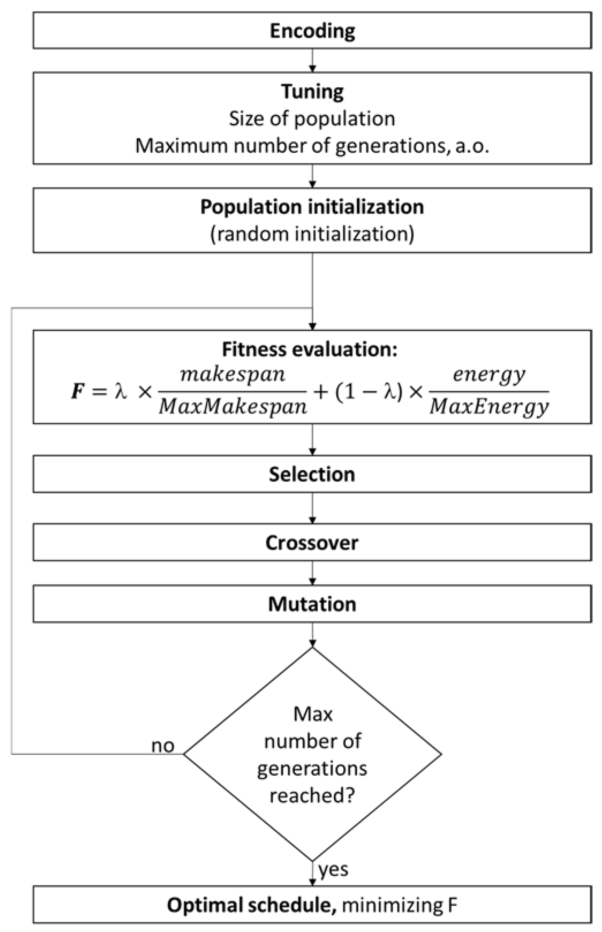
3.2. Genetic Algorithm (GA)

In this article, we propose to use a classical GA for the initial solving of FJSSP [38]. It is an optimization method based on an evolutionary process. The performance validation of the proposed algorithm is detailed in Section 5.1.

The aim of the FJSSP is to find a feasible schedule that minimizes makespan and energy consumption at the same time. Therefore, makespan and energy consumption are integrated into one objective function (F) using a weighted sum approach. The relative importance of each objective can be modified in F, which represents the fitness of the GA. Since the values of energy consumption and makespan are not proportional, we have to normalize both measures [39]. As presented in equation 1, makespan is divided by MaxMakespan, which is the maximum makespan value for the given problem, and energy consumption is divided by the MaxEnergy, which is the sum of the energy needed to execute all tasks of the problem. λ is the weight that reflects the importance of each objective function, λ ∈ [0…1]. This weight is modified statically, in this work. A dynamic evolution of λ is out of the scope of this article, and future perspectives may consider using an agent that controls the energy availability and triggers a rescheduling order when a threshold is reached.

$$F=\lambda \times \frac{makespan}{MaxMakespan}+(1-\lambda )\times \frac{energy}{MaxEnergy}$$

(1)

A flow chart illustrating the process of the genetic algorithm is represented in Figure 1. The overall structure of GA can be described in the following steps:

• Encoding: Each chromosome represents a solution for the problem. The genes of the chromosomes describe the assignment of operations to the machines, and the order in which they appear in the chromosome describes the sequence of operations.
• Tuning: The GA includes some tuning parameters that greatly influence the algorithm performance such as the size of population, the number of generations, etc. Despite recent research efforts, the selection of the algorithm parameters remains empirical to a large extent. Several typical choices of the algorithm parameters are reported in [40,41].
• Initial population: a set of initial solution is selected randomly.
• Fitness evaluation: A fitness function is computed for each of the individuals, this parameter indicates the quality of the solution represented by the individuals.
• Selection: At each iteration, the best chromosomes are chosen to produce their progeny.
• Offspring generation: The new generation is obtained by applying genetic operators like crossover and mutation
• Stop criterion: when a fixed number of generations is reached, the algorithm ends and the best chromosome, with their corresponding schedule, is given as output. Otherwise, the algorithm iterates again steps 3–5.

3.3. Disturbances in FJSSP

FJSSP considers a large variety of disturbances. These perturbations are random and uncertain and will bring instability to the initial schedule. In this work, one of the most common and frequent disruption in production scheduling will be considered: machine failures. We will deal with these events using rescheduling methods that will be discussed in the next section. These methods will try to maintain the stability of the system.

To simulate a machine failure [3], we have to select:

• The moment when the failure occurs (rescheduling time). These failures are randomly occurring, with a uniform distribution between 0 and the makespan of the original schedule generated with GA algorithm.
• The machine failing.
• The breakdown duration, which obeys to a uniform distribution between 25% and 50% of the makespan.

To simplify the problem, some assumptions about machine failures are considered:

• There is only one broken-down machine at a time.
• The time taken to transfer a job from the broken-down machine to a properly functioning machine is neglected.
• Machine maintenance is immediate after the failure.

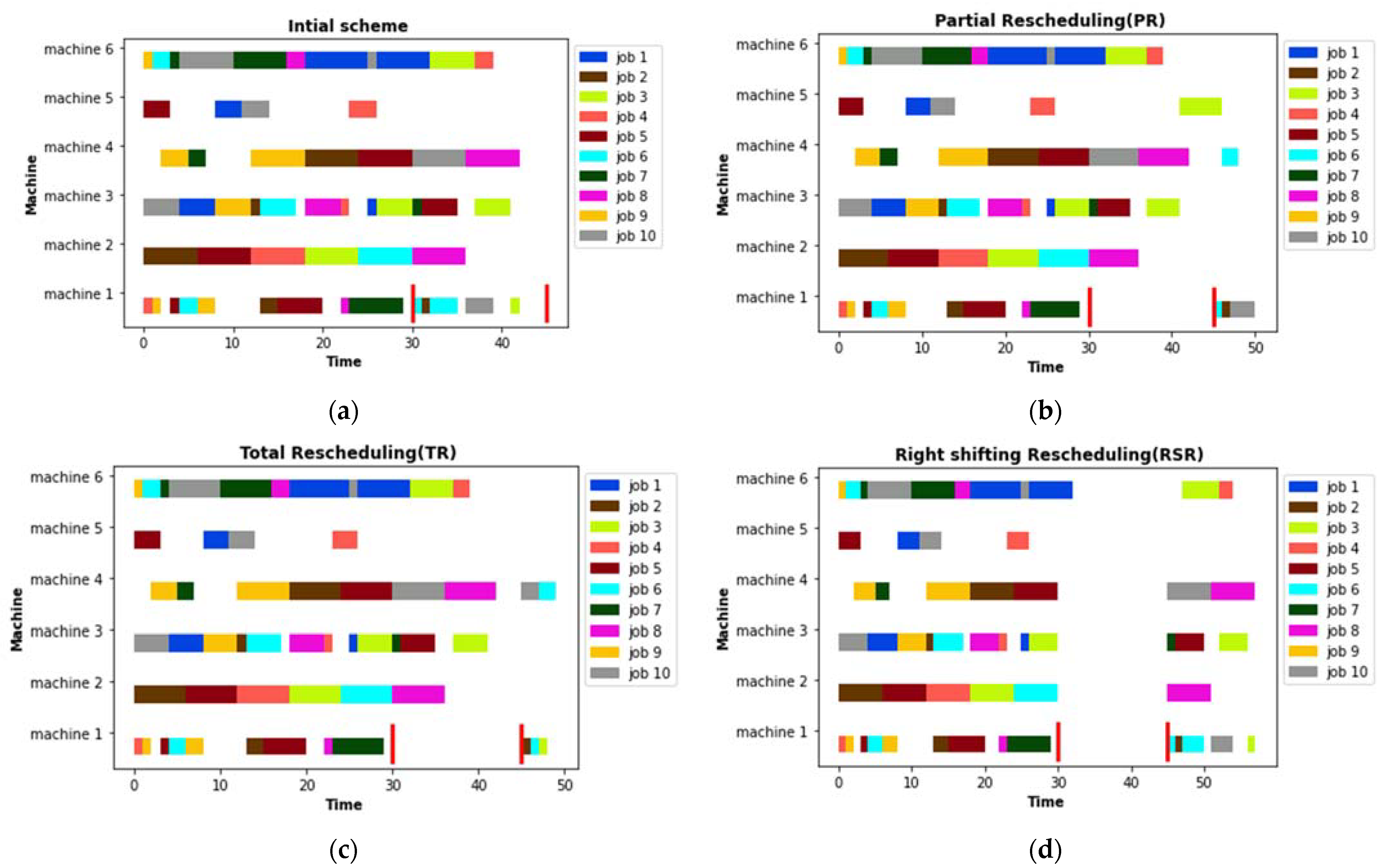
3.4. Rescheduling Strategies

One question can arise when dealing with the system disturbances, or the changed production circumstances: what kind of rescheduling methodologies should be used to produce a new schedule for the disturbance scenario? In the literature, many rescheduling methodologies were reported. Researchers classified these methods into two categories: (i) repairing a schedule that has been disrupted and (ii) creating a schedule that is more robust with respect to disruptions [42,43].

There are common methods used to repair a schedule that is no longer feasible due to disruptions: right shifting rescheduling, partial rescheduling, and total rescheduling. Their definitions are described respectively as follows [24]:

• Right shifting rescheduling (RSR): postpone each remaining operation by the amount of time needed to make the schedule feasible.
• Partial rescheduling (PR): reschedule only the operations affected directly or indirectly by the disturbances and preserve the original schedule as much as possible.
• Total rescheduling (TR): reschedule the entire set of operations that are not processed before the rescheduling point.

The choice of the most appropriate methodology depends on the nature of the perturbation and is generally made by experts. Rescheduling methods have different advantages and drawbacks: RSR and PR can quickly respond to machines’ breakdowns, however TR can offer a high-performance rescheduling, but with excessive computational effort. In this work, the targeted rescheduling strategy is the optimal one that minimizes the makespan and the energy consumption.

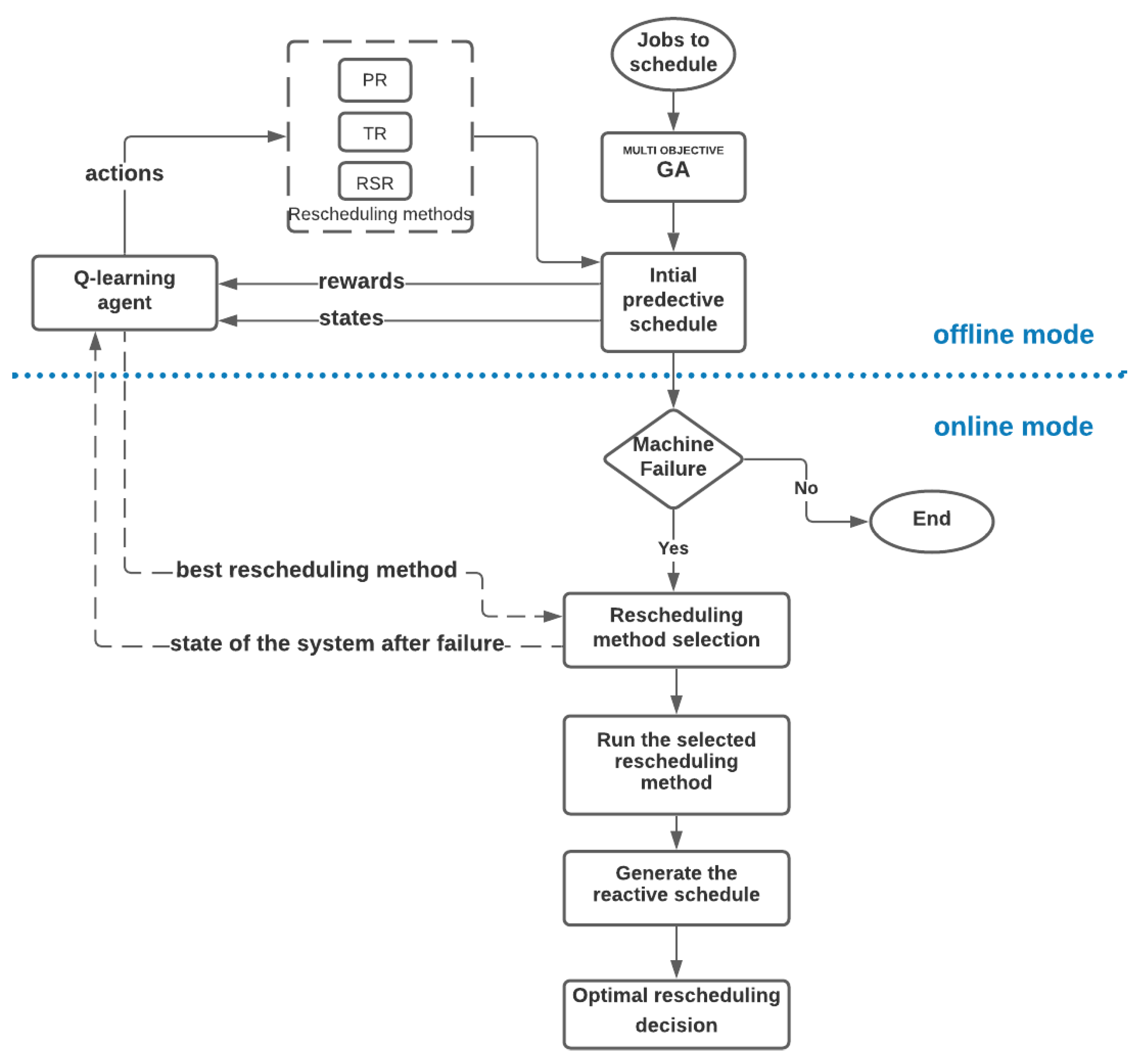
4. Proposed Multi Objective Q-Learning Rescheduling Approach

The proposed Q-learning-based rescheduling is described in Figure 2. The system is composed of two modes:

• An offline mode: in the first place the predictive schedule is obtained using a genetic algorithm, which represents the environment of the Q-learning agent. By interacting with this schedule and simulating experiments of machine failures, this agent learns how to select the optimal rescheduling solution for different states of the system.
• An online mode: when a machine failure occurs, the state of the system at the time of the interruption is delivered to the Q-learning agent. It responds by selecting the optimal rescheduling decision for this particular type of failure.

A key aspect of RL is that an agent has to learn a proper behavior. This means that it modifies or acquires new behaviors and skills incrementally [44]. An improvement of the Q-learning algorithm was also made to consider different criteria (multi-objective Q-learning). Next sections detail this algorithm.

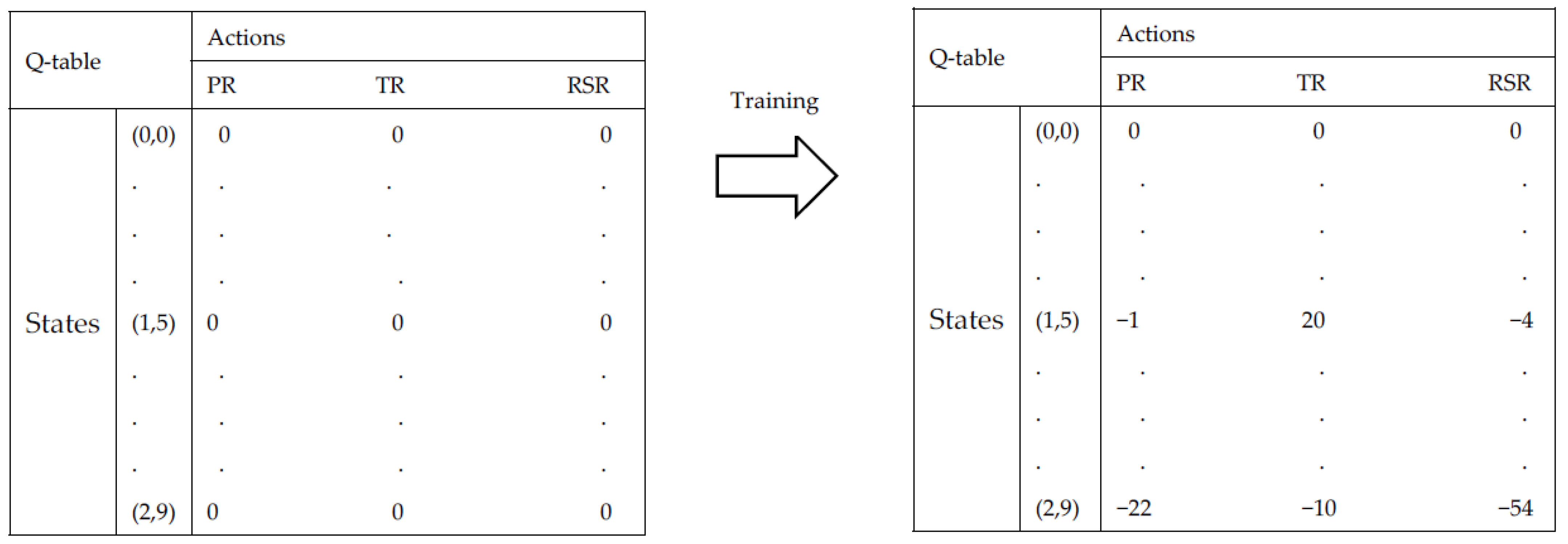
4.1. Q-Learning Terminologies

In order to be more accurate in the description of the algorithm, some terminologies of Q-learning are recalled below [45]:

• Agent: The agent interacts with its environment, selects its own actions, and responds to those actions;
• States: The set of environmental states S is defined as the finite set {$s^1$,...,$s^N$}, where the size of the state space is N;
• Actions: The set of actions A is defined as the finite set {$a^1$,...,$a^k$}, where the size of the action space is K. Actions can be used to control the system’s state;
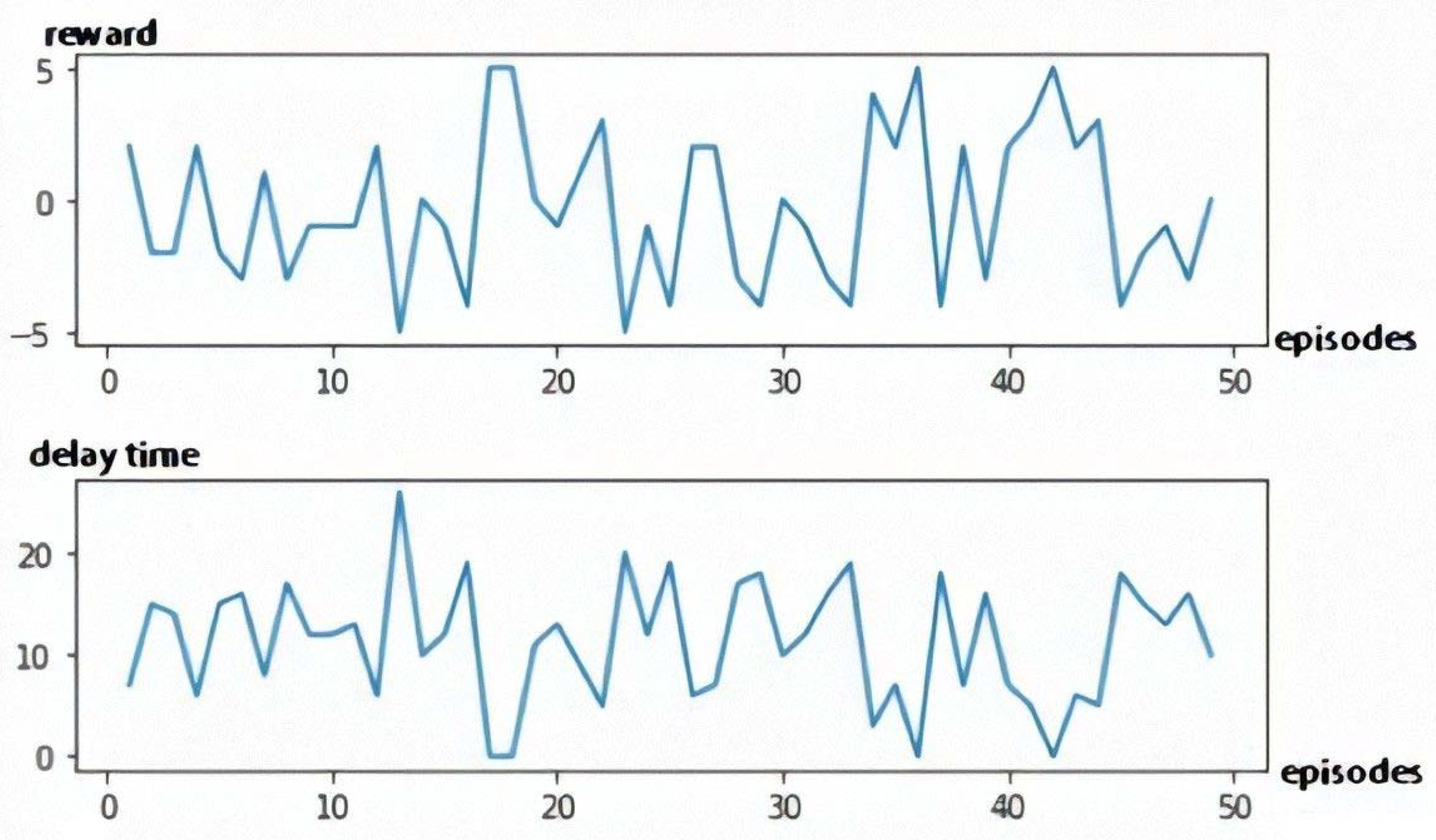
• Reward function: The reward function specifies rewards for being in a state or doing some action in a state.

To sum up, the agent will make optimal decisions using experiences, make an action in a particular state, and evaluate its consequences based on a reward. This process is done repeatedly until it becomes able to choose the best decision.

Q-learning is a value-based learning algorithm; it updates the value function based on a Bellman equation. The ‘Q’ here stands for quality of an action. The agent maintains a table of Q(s, a), updated along time based on Equation (2):

$$Q(s_t,a_t)=(1-\alpha ) Q(s_t,a_t)+\alpha ( r_{t+1}+\gamma \mathit{maxQ}(s_{t+1},a_{ }\left)\right)$$

(2)

where $r_{t+1}$ is the reward received when the agent transferring from the state $s_t$ to the state $s_{t+1}$, α is the learning rate (0 < α ≤ 1) (representing the extent to which our Q-values are being updated in every iteration), and γ is the discount factor (0 ≤ γ ≤ 1) (determining what importance is given to future rewards).

The algorithm of Q-learning is detailed in Algorithm 1.

Algorithm 1 Q-Learning

$\mathrm{Initialize} Q(s_{ }$$, A{a}_{ }$) randomly

Repeat for each episode:

Initialize s

Repeat for each step of episode

Choose an action from a using a policy derived from Q (ε-greedy)

Take an action a and observe the reward R and the next state s’

Update

Q$(s_t$,$a_t$$)=(1-\alpha ) Q(s_t$,$a_t$$)+\alpha ( r_{t+1}$$+\gamma \mathit{maxQ}(s_{t+1}$, $a_{ }$))

s ← s′

until s is terminal

4.2. Multi-Objective Q-Learning

In this case the agent has to optimize two objective functions at the same time. Here, the reward will transform from a scalar value to a vector of the size of the number of objective functions:

$$R(s_{ }, a_{ })=[R_1(s_{ }, a_{ }),R_2(s_{ }, a_{ }) \dots \dots \dots \dots ..R_m(s_{ }, a_{ }\left)\right]$$

(3)

where m is the number of objective functions.

The same thing occurs with action-state value Q(s,a) which becomes also a m-dimensional vector which is defined as follow:

$$Q(s, a)=[Q_1(s_{ }, a_{ }), Q_2(s_{ }, a_{ }) \dots \dots \dots \dots ..Q_m(s_{ }, a_{ }\left)\right]$$

(4)

where every value corresponds to a reward value from the reward vector.

In this article a multi-objective Q-learning with single policy approach is used. This means that it reduces the dimensionality of the multi-objective function. This new function fairly represents the importance of all objectives. For the single policy approach, many methods have been proposed. The most well-known is the weighted sum approach where scalarizing function is applied to Q(s, a) to acquire a scalar value $\overline{Q\left(s_{ }, a_{ }\right) }$ that considers all the objective functions. The linear scalarizing function is used and described as follows:

$$\overline{Q\left(s_{ }, a_{ }\right) }={{\displaystyle \sum }}_{i=0}^m{Q}_i\left(s_{ }, a_{ }\right)]\ast w_i$$

(5)

where $0\le w_i\le 1$ is the weight that specifies the importance of each objective function, and must satisfy the following equation: ${{\displaystyle \sum }}_{i=0}^m{w}_i=1$

The algorithm of the multi-objective Q-learning is detailed in Algorithm 2.

Algorithm 2 Multi-Objective Q-Learning

$\mathrm{Initialize} Q(s_{ }$$, a_{ }$) randomly

Repeat for each episode:

Initialize s

Repeat for each step of episode

Choose an action from a using a policy derived from Q (ε-greedy)

$\mathrm{Take} \mathrm{an} \mathrm{action} \mathrm{a} \mathrm{and} \mathrm{observe} \mathrm{the} \mathrm{rewards} R_1$$\mathrm{and} R_2$ and the next state s’

Update

$Q_1$$(s_t$, $a_t$$)=(1-\alpha ) Q_1$$(s_t$, $a_t$$)+\alpha (R_1{}_{t+1}$ + γ max$Q_1$ $(s_{t+1}$, $a_{ }$))

$Q_2$($s_t$, $a_t$$)=(1-\alpha ) Q_2$ $(s_t$, $a_t$$)+\alpha (R_2{}_{t+1}$ + γ max$Q_2$ $(s_{t+1}$, $a_{ }$))

s ← s′

until s is terminal

4.3. State Space Definition

The state space is the set of all possible situations the agent could inhabit. We have to select the number of states that will give the optimal solution and how to define these states. In this article, two indicators were used to establish the state space:

• s1: indicates the moment when the perturbation happens, e.g., in the beginning, the middle or in the end of the schedule. For this purpose, the initial makespan was divided into 3 intervals, so s1 can take the values 0, 1 or 2.
• s2: defined by the indicator SD which is the ratio of the duration of the directly affected operation by the machine’s breakdown to the total processing time of the remaining operations on failed machine. The formula is described as follows:

$$\mathit{SD}=\frac{O_{aff}}{RT}\ast 100$$

(6)

where O_aff is the directly affected operation by the breakdown machine and RT is the total processing time of the remaining operations on failed machine. s2 is an integer between 0 and 9 depending on the value of SD.

The couple (s1, s2) represents the state of the system at a particular time, given the rescheduling time, the failure machine, and the breakdown duration. In total we have 30 states, where 0 ≤ s1 ≤ 2 and 0 ≤ s2 ≤ 9 (s1 and s2 are integers).

4.4. Actions and Reward Space Definition

The agent encounters one of the 30 states, and it takes an action. The action in this case is one of the rescheduling methods:

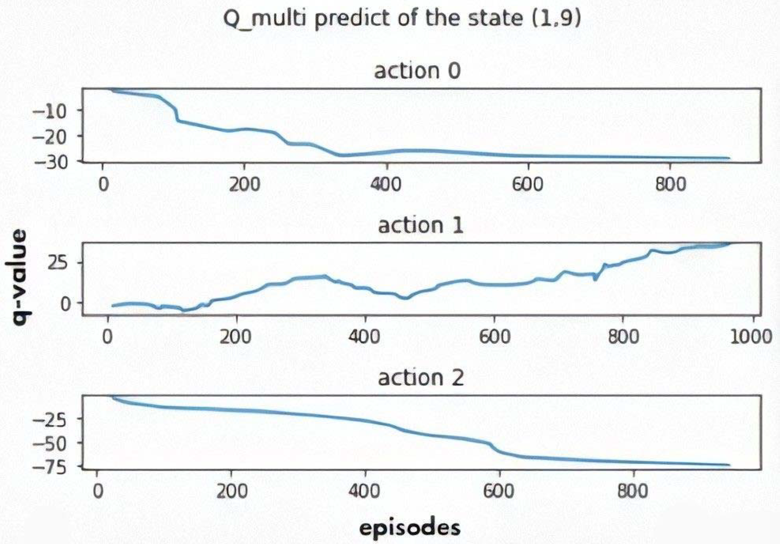
• Action 0: Partial rescheduling (PR)
• Action 1: Total rescheduling (TR)
• Action 2: Right shifting rescheduling (RSR)

The definition of the reward plays an important role in the algorithm since the Q-learning agent is reward-motivated. This means that it selects the best action by evaluating the reward. In this work, the reward is a vector with two scalars

$$R(s_{ },a_{ })=[R_1(s_{ },a_{ }), R_2(s_{ },a_{ }\left)\right]$$

(7)

where $R_1$($s_{ }$,$a_{ }$) depends on delay time (the longer the delays, the smaller the rewards) and $R_2$(${\mathrm{s}}_{ }$,$a_{ }$) depends on the difference of energy consumption between the initial scheme and the scheme after rescheduling (the bigger these differences, the smaller the rewards). The rewards are set to be between 5 and −5, based on how much delay time there is and the difference in energy consumption the action will cause.

5. Experiments and Results

In order to evaluate the performance of the proposed model, benchmark problems are used. At the authors’ best knowledge, there are currently no benchmarks available in the literature considering energy in an FJSSP. Therefore, instances had to be created in order to test and validate this work. The choice was made to extend classical problems from the literature to support energy consumption. The chosen problems are taken from Brandimarte [46]. This consists of 10 problems (mk1 to mk10), where the jobs range from 10 to 20 operations, machines from 6 to 15, and operations for each job from 5 to 15. An energy consumption of every operation was added randomly, obeying a uniform distribution between 1 and 100. Thus, for each instance, the machining energy consumption and the idle power of machines are specified as inputs.

In this article, the unit of the makespan is unit of time and the unit of the energy consumption is in kWh.

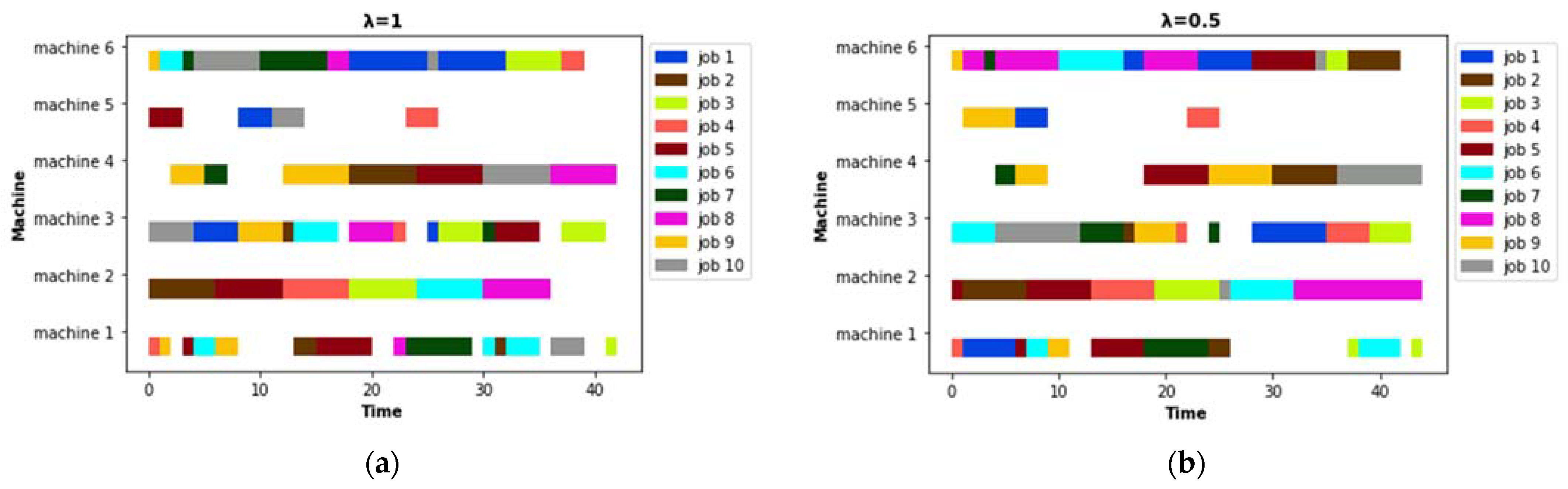
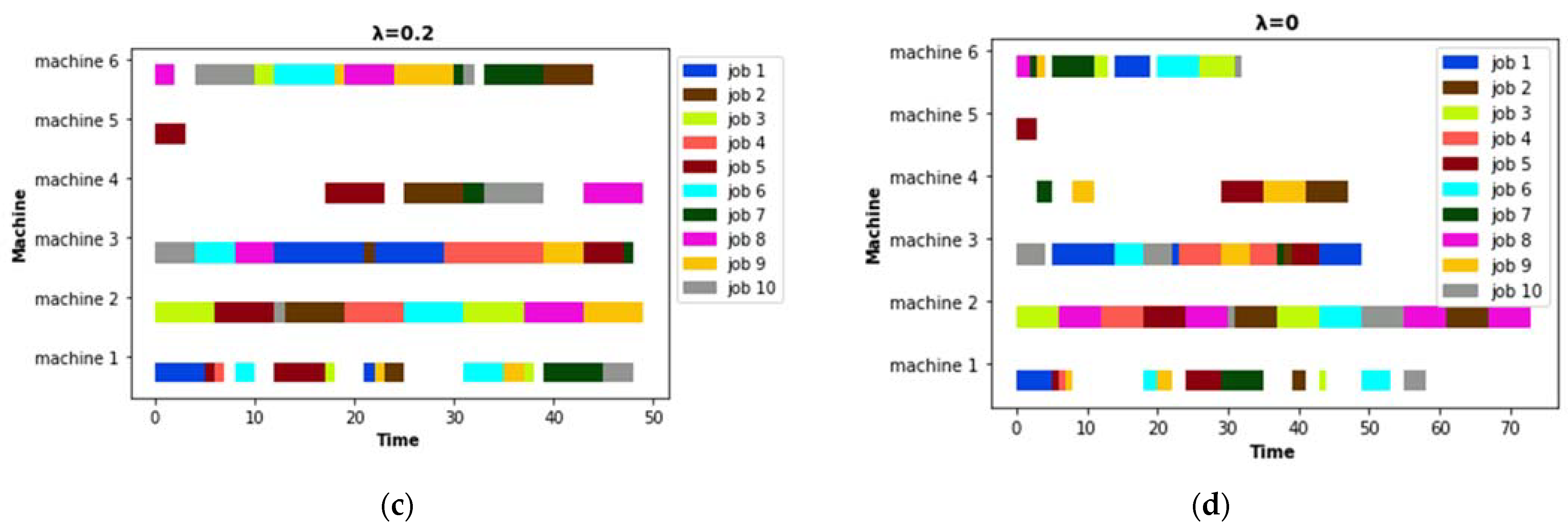
5.1. Predictive Schedule Based on GA

Initially, the optimal scheduling scheme is acquired based on GA. Python programming is used to develop the proposed method using the distributed evolutionary algorithms in python framework (DEAP), which is a novel evolutionary computation framework. The parameters of GA are set as follows: the size of initial population is 50 and the number of generations is 500.

To validate the GA, a comparison with other methods in literature was made, such as PSO proposed by [47] and TS proposed by [48]. The result of the Brandimarte instances in terms of makespan of these different algorithms is presented in

Table 3. Results in terms of makespan (in time units) of the Brandimarte instances for different algorithms.

Instances	The Proposed GA	PSO by [47]	TS by [48]
Mk01	42	41	42
Mk02	32	26	32
Mk03	206	207	211
Mk04	67	65	81
Mk05	179	171	186
Mk06	86	61	86
Mk07	164	173	157
Mk08	523	523	523
Mk09	342	307	369
Mk10	292	312	296

Italics here identify the most effective algorithm through the lowest value of the makespan.

. The weight of the objective function of genetic algorithm is set to 1, to give importance to makespan rather than energy reduction.

As can be seen from Table 3, the proposed GA gives similar results to PSO and TS algorithm when the weight is set to 1. Therefore, we consider this proposition as satisfying.

In the next step, more importance is given to energy reduction, therefore the weight of the objective function is modified. The Gantt chart of the predictive schedule using GA of Mk01 for different weight values is shown in Figure 3.

The makespan and energy consumption values for different cases are described in

Table 4. Makespan (MK in time units) and energy consumption (EC in kWh) calculation example on MK01 instance.

Instance	Size	Weight	KPIs
			MK	EC
MK01	10 × 6	1	42	2812
		0.5	44	2457
		0.2	49	2411
		0	73	2229

. This shows that the two objective functions are antagonistic. When the weight is set to 1, importance is given to makespan, therefore in this case GA provides the best makespan (42) but the biggest energy consumption value (2812). On the opposite, when the weight is set to 0, the importance is given to energy reduction, in this case GA provides the worst makespan (73) but the best energy consumption value (2229). It may be noted that when the weight decreases, makespan decreases but energy consumption increases.

5.2. Rescheduling Strategies

To illustrate the difference between the different rescheduling methods presented in Section 3.4, the predictive schedule of the instance MK01 where the weight is set to 1 is taken as example. A random perturbation (machine failure) is applied, assuming that at time t = 20, machine 1 is broken down and t′ = 6 is the duration of the breakdown. The new schedules acquired by the three rescheduling methods (PR, TR and RSR) are presented in Figure 4, the red line representing the starting time and ending time of machine failure.

The directly affected operations by the failure machine are $O_{5,6}$, $O_{6,2}$, $O_{6,6}$, $O_{6,10}$,$\mathrm{and} O_{6,3}$, these operations are executed by the broken-down machine. In PR, $O_{5,6}$, $O_{6,2}$, $O_{6,10}$ are postponed after the breakdown and the $O_{6,6}$ and $O_{6,3}$ are executed respectively on machine 4 and 5 with a different processing time (Figure 4b). In TR, all the remaining jobs are rescheduled using the GA algorithm after the breakdown (Figure 4c). As for RSR, all the remaining jobs are postponed by the breakdown duration (Figure 4d). The performance of the rescheduling methods is described in the

Table 5. The makespan (time units) and energy consumption (kWh) calculation for rescheduling methods on MK01 instance.

Schedule		Makespan (MK)	Energy Consumption(EC)
Predictive schedule		42	2812
Reactive schedule	PR schedule	50	3046
	TR schedule	49	2895
	RSR schedule	57	2887

.

As can be seen from Table 5, the three rescheduling methods gives different results. Both makespan and energy consumption are increased due to the presence of the machine failure that affects a set of operation. In terms of makespan, TR gives the best result (42), but in terms of energy consumption, RSR gives the best result (2887). This result can be explained by the date of the failure, which happened close to the end of the initial schedule.

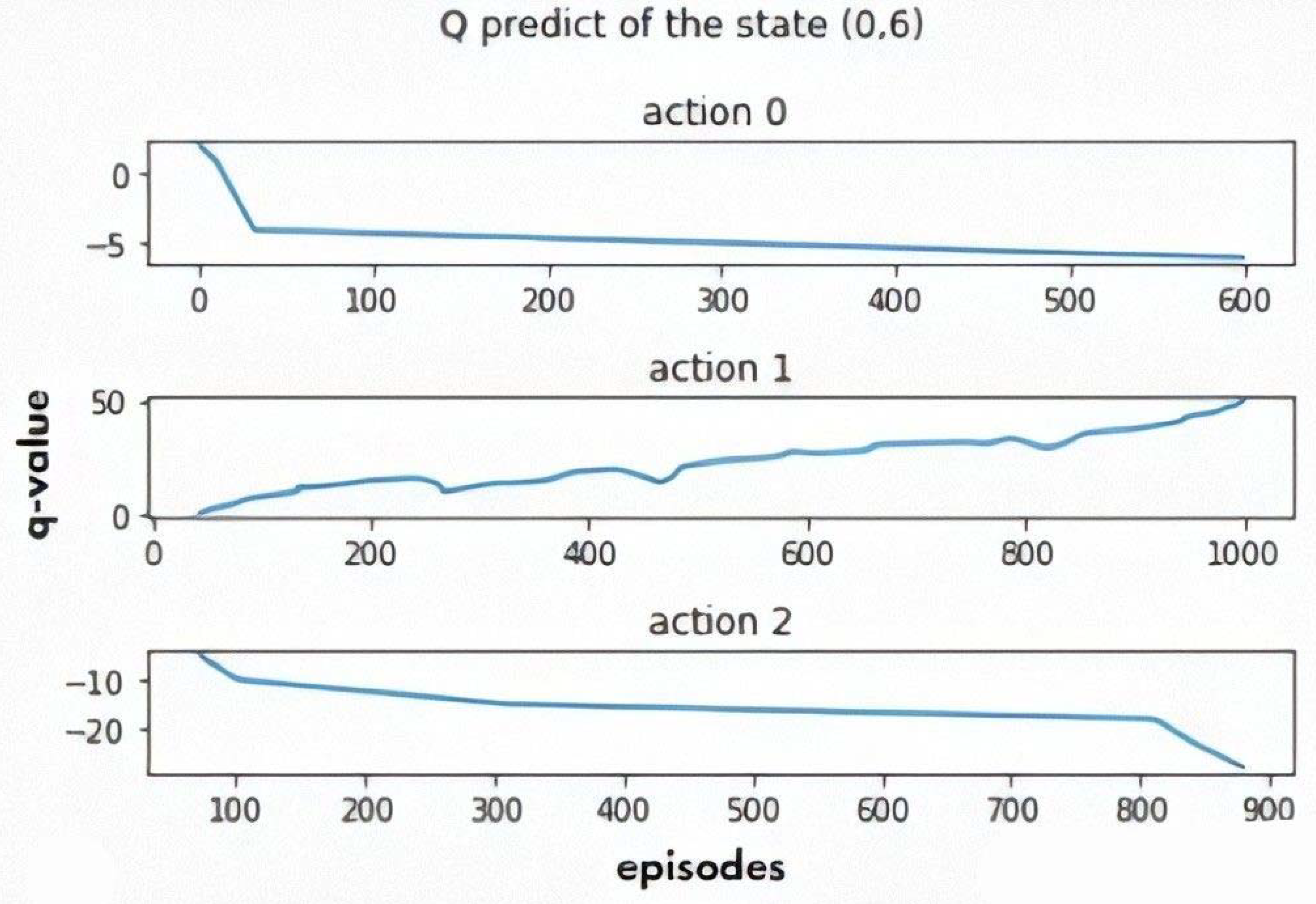
5.3. Rescheduling Based on Q-Learning

To test the performance of the proposed Q-learning algorithm, we designed simulation experiments of machine failures. The parameters are set as follows:

• α = 1: A learning rate of 1 means the old value will be completely discarded, the model converges quickly, no large number of episodes are required;
• γ = 0: The agent considers only immediate rewards. In each episode, one state is evaluated (the initial state of the system at a particular time, given the rescheduling time, the failure machine and the breakdown duration)
• ε = 0.8, the balance factor between exploration and exploitation. Exploration refers to searching over the whole sample space while exploitation refers to the exploitation of the promising areas found. In the proposed model, 80% is given to exploitation, so in 80% of cases the agent will choose the action with the biggest reward and in 20% of cases he will randomly choose an action to explore more of its environment.
• The number of episodes is 1000, for the model to converge.

In each episode the Q-table is updated depending on the value of the rewards (Figure 5).

5.3.1. The Single Objective Q-Learning

Two types of Q-learning algorithm are proposed in this article: the single objective Q-learning and multi-objective Q-learning.

The aim of the single objective function Q-learning is to minimize the makespan, which means the minimization of the delay time. The curve of the reward and the delay time in the first 50 episodes are described in Figure 6. It can be seen that the longer the delay time, the lower the reward value.

To show how the Q-values are updated in each episode, the state (0.7) is taken as example. Figure 7 describes the variation of Q-values of each action. The agent first selects the action 0 and gets a positive reward so its Q-value increases. After a few episodes, action 0 is chosen again because it has the biggest Q-value but gets a negative reward. Its Q-value thus decreases, giving the chance for action 1 to be selected. After that, action 1 is chosen in every episode because it gets a positive reward each time so its Q-value increases. Action 2 is selected in ${100}^{\mathrm{th}}$ and ${800}^{\mathrm{th}}$ episodes due to the ε-greedy where the agent still has a 20% probability to explore but its Q-value decreases because it gets negative rewards.

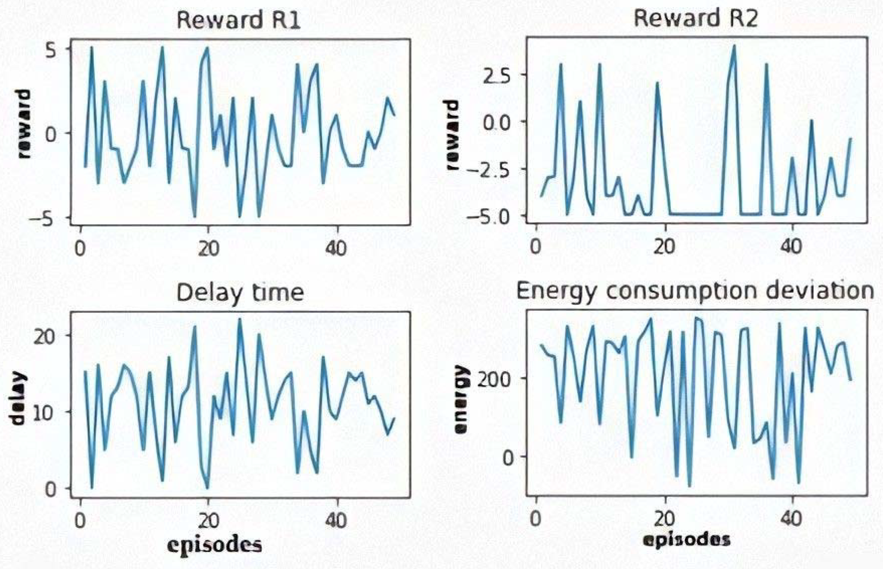
5.3.2. The Multi-Objective Q-Learning

The goal of the multi-objective Q-learning approach is to minimize the makespan and the energy consumption at the same time. In this case, two rewards are considered: reward $R_1$ that depends on the delay time and reward $R_2$ that depends on the energy consumption deviation. Figure 8 describes the variation of the reward along the first 50 episodes. It can be seen that ${\mathrm{R}}_1$increases when the delay time decreases and $R_2$ increases when the energy consumption deviation decreases.

This time, state (1.9) is taken as an example and the weight of the objective function of the multi Q-learning algorithm is set to 0.5 (which means that makespan and energy consumption have the same importance). Throughout the episodes, action 1 gets positive rewards and its Q-value increases so it is selected most of the times, on the other hand action 0 and action 2 get negative rewards so their Q-values decrease, they are chosen only in the exploration phase. The Q-value prediction of the state (1.9) is presented in Figure 9.

5.4. Models Validation

The results of the optimal rescheduling methods for the Brandimarte [46] instances and the solution given by the Q-learning agent are represented in Appendix A. In

Table 6. Performance measurement of the predictive and reactive schedule in MK01 instance.

Instance	Size	p	Weight of BF	Predictive Schedule		Machine Failure			State of the System	Reactive Schedule						Q-Learning
										PR		TR		RSR		Single Objective	Multi-Objective
				MK (Time Units)	EC (kWh)	Failure Time	Broken-Down Machine	Failure Duration		MK (Time Units)	EC (kWh)	MK (Time Units)	EC (kWh)	MK (Time Units)	EC (kWh)
MK01	10 × 6	2	1	42	3046	3	5	20	(0.5)	46	3064	45	3115	61	3160	TR	TR
						16	4	19	(1.9)	60	3128	55	3243	66	3180	TR	TR
						8	1	17	(0.6)	57	3099	50	3190	58	3142	TR	TR
						23	3	14	(1.7)	57	3101	56	3218	58	3142	TR	TR
						13	5	10	(0.4)	46	3058	45	3028	52	3106	TR	TR
						13	6	20	(0.9)	56	3098	54	3204	59	3148	TR	TR
			0.5	49	2837	11	1	12	(0.5)	54	2872	58	2826	61	2909	TR	TR
						7	5	23	(0.9)	56	2890	57	2724	76	2999	PR	TR
						22	2	22	(1.9)	62	2950	56	2968	65	2993	TR	TR
						5	2	12	(0.3)	54	2935	54	2853	55	2939	TR	TR
						11	1	12	(0.6)	54	2872	58	2826	61	2909	PR	PR
						13	4	13	(0.2)	50	2839	54	2816	54	2867	PR	PR
			0.2	52	2672	31	2	15	(1.9)	64	2702	67	2711	67	2672	PR	PR
						4	2	20	(0.4)	75	2797	78	2757	75	2800	TR	PR
						10	4	14	(0.0)	52	2673	58	2670	59	2714	PR	PR
						10	1	21	(0.6)	64	2728	68	2632	73	2798	TR	PR
						20	2	22	(1.7)	72	2769	76	2773	75	2820	PR	PR
						6	5	26	(0.9)	65	2727	68	2704	74	2804	PR	TR
			0	79	2554	23	6	20	(0.9)	91	2649	99	2612	102	2692	PR	TR
						1	5	26	(0.3)	79	2560	79	2574	102	2686	PR	PR
						31	2	37	(1.8)	92	2668	110	2706	116	2776	PR	PR
						3	2	24	(1.6)	88	2639	100	2666	106	2689	PR	PR
						16	2	34	(0.6)	98	2700	110	2744	116	2776	PR	PR
						30	6	20	(1.9)	79	2564	79	2605	98	2668	PR	PR

, an extraction of Appendix A, corresponding to the instance MK01, is taken as example. The first column is the name of the instance, followed by its size and its level of flexibility. In the fourth column, the weight of the objective function of the GA and of the multi-objective Q-learning is defined. In the fifth column, makespan and energy consumption of the predictive schedule are calculated. In the sixth column, different types of machine failures are defined by their failure time, the reference of the failing machine and the failure duration. Next comes the state definition, then the rescheduling methods and their performance. In the last column the evaluated Q-learning approach is presented by giving the makespan (MK) and the energy consumption (EC) of the selected optimal rescheduling solution using single objective Q-learning and multi-objective Q-learning.

In the predictive schedule, when the weight decreases, the makespan increases but the energy consumption decreases. This is normal because importance is given to energy consumption each time the weight is decreased. After simulating different types of failure randomly, it can be seen that the Q-learning is able to choose the best rescheduling methods each time; the single objective Q-learning selects the best methods that minimize the makespan but the multi objective Q-learning selects the best methods that minimize the makespan and energy consumption depending on the value of the weight of the objective function.

When this weight is set to 1, the single objective and multi-objective Q-learning have the same results. They both choose the methods that minimize the makespan regardless of the value of the energy consumption. From

Table 7. CPU time comparison.

Instances	CPU Time (s)
	Traditional Rescheduling	Q-Learning
MK01	6.173	0.001
MK02	7.261
MK03	45.068
MK04	13.680
MK05	24.488
MK06	48.855
MK07	30.716
MK08	61.261
MK09	85.610
MK10	84.545

, in the case of the MK01, TR proved to have the highest performance and was selected in both algorithms. Giving the same importance to energy consumption, which implies setting the value of the weight to 0.5, the selected method changes to make a compromise between the two objectives. There is a difference between the result of single objective and multi-objective Q-learning. Taking the state (0.9) as example, PR and TR gives 56 and 57 as makespan respectively and 2890 and 2724 as energy consumption respectively, so PR is selected by the single-objective Q-learning because it generates the minimum makespan, but TR is selected by the multi-objective Q-learning because it has better result than PR in terms of energy consumption.

By further decreasing the value of the weight to 0.2, more prominence is given to energy consumption. Taking the example of the state (0.4), PR and TR give 75 and 79 as makespan respectively and 2797 and 2757 as energy consumption respectively. Here PR is selected by the single objective Q-learning because it minimizes the makespan, but TR is selected by the multi-objective Q-learning because it has better optimization of the energy consumption that was given more importance. Once the weight is set to 0, the multi-objective Q-values selects the methods that optimizes the energy consumption regardless of the value of the makespan, as in state (0.9) when PR gave the best makespan (91) so it was selected by the single-objective Q-learning, but TR was selected by the multi-objective Q-learning because it gave the best energy consumption (2612).

Considering all the instances of the Brandimarte benchmark, in Appendix A, we can also deduce that the right shift rescheduling turned out to have the worst performance, this is due to the postponement of the remaining tasks which increases both the makespan and the energy variation. Another deduction that can be taken is that generally TR have the best performance in early failures and PR gives better results when the failures occur in the middle or in the end of the schedule and especially with instances that have high flexibility. The results of RSR also become improved at the end of the schedule because the number of postponed operations is smaller.

The Q-learning algorithm not only selects the optimal methods for rescheduling but also responds immediately to perturbation. Table 7 indicates the CPU time comparison between the time spent to execute the three rescheduling methods (PR, TR, RSR) and to select the optimal one and the time spent by the Q-learning algorithm to select the best method from the Q-table. The reported values are evaluated using a laptop computer with Intel core i5-8250U with 1.8 GHZ speed and with 12 Gb memory. The offline training of the Q-learning algorithm can take minutes or even some hours depending on the instance size, but it can be seen that, in online execution, the learning-based rescheduling selection of the optimal solution takes only one millisecond compared with traditional rescheduling that can exceed one minute, this time corresponds to state calculation of the system after perturbation and the selection of the best methods that have the highest Q-values from the corresponding Q-values table. However, the execution of the three rescheduling methods and the selection of the best method can take several seconds, even minutes when the instance is large.

6. Conclusions

This work deals with the flexible job shop scheduling problem under uncertainties. A multi-objective Q-learning rescheduling approach is proposed to solve the FJSSP under machine failures. Two key performance indicators are used to select the best schedule: the makespan and the energy consumption. The idea was not only to maintain effectiveness but also to improve energy efficiency. The approach is hybrid and combines predictive and reactive phases. The originality of this work is to combine AI and scheduling techniques to be able to rapidly solve a bi-objectives problem (makespan and energy consumption) of rescheduling in a context of FJSP.

First, a genetic algorithm was developed to provide an initial predictive schedule that minimizes the makespan and energy consumption simultaneously. In this predictive phase, different types of machine failures were simulated and classical rescheduling policies (RSR, TR, PR) were executed to repair the predictive scheduling and to find new solutions. Based on these results, the Q-learning agent is trained. To consider the energy consumption even in the rescheduling process, a multi-objective Q-learning algorithm was proposed. A weighting parameter is used to make a tradeoff between the makespan and the energy consumption. In the reactive phase, the Q-learning agent is tested on new machine disruptions. The Q-learning agent seeks to find the best action to take given the current state. In fact, the main goal of using AI tools is to be able to react quickly facing failures while rapidly selecting the best rescheduling policy related to the state of the environment. In order to assess the performance of the developed approach, the Brandimarte [46] benchmark was extended to support energy consumption. On this new benchmark, the Q-learning based rescheduling approach was tested to respond to unexpected machine failures and select the best rescheduling strategy.

The results of this study show that the approach proved to be effective in responding quickly and accurately to unexpected machine failures. The Q-learning algorithm provided appropriate strategy choices based on the state of the environment with various balance between the objectives of energy consumption and productivity. The learning phase was therefore efficient enough to enable these efficient choices. The choices of genetic algorithm and Q-learning algorithm proved their efficiency on the extended classical instances of Brandimarte in this work. Nevertheless, the approach leaves the possibility to the user to integrate their own choice of algorithm according to the specific context.

Future works are oriented to take into consideration other types of disruptions like new job insertions, variety of availability of energy, urgent job arrivals, etc. Another future perspective that can be expected is the evaluation of the proposed approach on other types of learning techniques in order to compare with the Q-learning algorithm. On a more global perspective, this work contributes to the development of efficient rescheduling approaches for the control of future industrial systems. Such systems are meant to integrate more and more flexibility, and the performance evaluation of this work on a FJSP shows the compatibility of the approach with this objective. This work also contributes to the integration of multi-objective rescheduling strategies in industry, which is especially relevant for sustainability concerns.

References

- Giret, A.; Trentesaux, D.; Prabhu, V. Sustainability in Manufacturing Operations Scheduling: A State of the Art Review. J. Manuf. Syst. 2015, 37, 126–140. [Google Scholar] [CrossRef]
- Zhang, L.; Li, X.; Gao, L.; Zhang, G. Dynamic Rescheduling in FMS That Is Simultaneously Considering Energy Consumption and Schedule Efficiency. Int. J. Adv. Manuf. Technol. 2016, 87, 1387–1399. [Google Scholar] [CrossRef]
- Nouiri, M.; Bekrar, A.; Trentesaux, D. Towards Energy Efficient Scheduling and Rescheduling for Dynamic Flexible Job Shop Problem. IFAC-Pap. 2018, 51, 1275–1280. [Google Scholar] [CrossRef]
- Masmoudi, O.; Delorme, X.; Gianessi, P. Job-Shop Scheduling Problem with Energy Consideration. Int. J. Prod. Econ. 2019, 216, 12–22. [Google Scholar] [CrossRef]
- Liu, Y.; Dong, H.; Lohse, N.; Petrovic, S. A Multi-Objective Genetic Algorithm for Optimisation of Energy Consumption and Shop Floor Production Performance. Int. J. Prod. Econ. 2016, 179, 259–272. [Google Scholar] [CrossRef] [Green Version]
- Kemmoe, S.; Lamy, D.; Tchernev, N. Job-Shop like Manufacturing System with Variable Power Threshold and Operations with Power Requirements. Int. J. Prod. Res. 2017, 55, 6011–6032. [Google Scholar] [CrossRef]
- Raileanu, S.; Anton, F.; Iatan, A.; Borangiu, T.; Anton, S.; Morariu, O. Resource Scheduling Based on Energy Consumption for Sustainable Manufacturing. J. Intell. Manuf. 2017, 28, 1519–1530. [Google Scholar] [CrossRef]
- Mokhtari, H.; Hasani, A. An Energy-Efficient Multi-Objective Optimization for Flexible Job-Shop Scheduling Problem. Comput. Chem. Eng. 2017, 104, 339–352. [Google Scholar] [CrossRef]
- Gong, X.; De Pessemier, T.; Martens, L.; Joseph, W. Energy-and Labor-Aware Flexible Job Shop Scheduling under Dynamic Electricity Pricing: A Many-Objective Optimization Investigation. J. Clean. Prod. 2019, 209, 1078–1094. [Google Scholar] [CrossRef] [Green Version]
- Chen, X.; Li, J.; Han, Y.; Sang, H. Improved Artificial Immune Algorithm for the Flexible Job Shop Problem with Transportation Time. Meas. Control 2020, 53, 2111–2128. [Google Scholar] [CrossRef]
- Salido, M.A.; Escamilla, J.; Barber, F.; Giret, A. Rescheduling in Job-Shop Problems for Sustainable Manufacturing Systems. J. Clean. Prod. 2017, 162, S121–S132. [Google Scholar] [CrossRef] [Green Version]
- Caldeira, R.H.; Gnanavelbabu, A.; Vaidyanathan, T. An Effective Backtracking Search Algorithm for Multi-Objective Flexible Job Shop Scheduling Considering New Job Arrivals and Energy Consumption. Comput. Ind. Eng. 2020, 149, 106863. [Google Scholar] [CrossRef]
- Xu, B.; Mei, Y.; Wang, Y.; Ji, Z.; Zhang, M. Genetic Programming with Delayed Routing for Multiobjective Dynamic Flexible Job Shop Scheduling. Evol. Comput. 2021, 29, 75–105. [Google Scholar] [CrossRef]
- Luo, J.; El Baz, D.; Xue, R.; Hu, J. Solving the Dynamic Energy Aware Job Shop Scheduling Problem with the Heterogeneous Parallel Genetic Algorithm. Future Gener. Comput. Syst. 2020, 108, 119–134. [Google Scholar] [CrossRef]
- Tian, S.; Wang, T.; Zhang, L.; Wu, X. An Energy-Efficient Scheduling Approach for Flexible Job Shop Problem in an Internet of Manufacturing Things Environment. IEEE Access 2019, 7, 62695–62704. [Google Scholar] [CrossRef]
- Nouiri, M.; Trentesaux, D.; Bekrar, A. EasySched: Une Architecture Multi-Agent Pour l’ordonnancement Prédictif et Réactif de Systèmes de Production de Biens En Fonction de l’énergie Renouvelable Disponible Dans Un Contexte Industrie 4.0. arXiv 2019, arXiv:1905.12083. [Google Scholar] [CrossRef] [Green Version]
- Bishop, C.M. Pattern Recognition and Machine Learning (Information Science and Statistics); Springer: Berlin, Germany, 2007. [Google Scholar]
- Shahzad, A.; Mebarki, N. Learning Dispatching Rules for Scheduling: A Synergistic View Comprising Decision Trees, Tabu Search and Simulation. Computers 2016, 5, 3. [Google Scholar] [CrossRef] [Green Version]
- Wang, C.L.; Rong, G.; Weng, W.; Feng, Y.P. Mining Scheduling Knowledge for Job Shop Scheduling Problem. IFAC-Pap. 2015, 48, 800–805. [Google Scholar] [CrossRef]
- Zhao, M.; Gao, L.; Li, X. A Random Forest-Based Job Shop Rescheduling Decision Model with Machine Failures. J. Ambient. Intell. Humaniz. Comput. 2019, 1–11. [Google Scholar] [CrossRef]
- Li, Y.; Carabelli, S.; Fadda, E.; Manerba, D.; Tadei, R.; Terzo, O. Machine Learning and Optimization for Production Rescheduling in Industry 4.0. Int. J. Adv. Manuf. Technol. 2020, 110, 2445–2463. [Google Scholar] [CrossRef]
- Pereira, M.S.; Lima, F. A Machine Learning Approach Applied to Energy Prediction in Job Shop Environments. In Proceedings of the IECON 2018-44th Annual Conference of the IEEE Industrial Electronics Society, Washington, DC, USA, 21–23 October 2018; pp. 2665–2670. [Google Scholar]
- Li, Y.; Chen, Y. Neural Network and Genetic Algorithm-Based Hybrid Approach to Dynamic Job Shop Scheduling Problem. In Proceedings of the 2009 IEEE International Conference on Systems, Man and Cybernetics, San Antonio, TX, USA, 11–14 October 2009; pp. 4836–4841. [Google Scholar]
- Wang, C.; Jiang, P. Manifold Learning Based Rescheduling Decision Mechanism for Recessive Disturbances in RFID-Driven Job Shops. J. Intell. Manuf. 2018, 29, 1485–1500. [Google Scholar] [CrossRef]
- Mihoubi, B.; Bouzouia, B.; Gaham, M. Reactive Scheduling Approach for Solving a Realistic Flexible Job Shop Scheduling Problem. Int. J. Prod. Res. 2021, 59, 5790–5808. [Google Scholar] [CrossRef]
- Adibi, M.A.; Shahrabi, J. A Clustering-Based Modified Variable Neighborhood Search Algorithm for a Dynamic Job Shop Scheduling Problem. Int. J. Adv. Manuf. Technol. 2014, 70, 1955–1961. [Google Scholar] [CrossRef]
- Sutton, R.S.; Barto, A.G. Reinforcement Learning: An Introduction; MIT Press: Cambridge, MA, USA, 2018. [Google Scholar]
- Riedmiller, S.; Riedmiller, M. A Neural Reinforcement Learning Approach to Learn Local Dispatching Policies in Production Scheduling. In Proceedings of the IJCAI, Stockholm, Sweden, 31 July–6 August 1999; Volume 2, pp. 764–771. [Google Scholar]
- Chen, X.; Hao, X.; Lin, H.W.; Murata, T. Rule Driven Multi Objective Dynamic Scheduling by Data Envelopment Analysis and Reinforcement Learning. In Proceedings of the 2010 IEEE International Conference on Automation and Logistics, Hong Kong and Macau, China, 16–20 August 2010; pp. 396–401. [Google Scholar]
- Gabel, T.; Riedmiller, M. Distributed Policy Search Reinforcement Learning for Job-Shop Scheduling Tasks. Int. J. Prod. Res. 2012, 50, 41–61. [Google Scholar] [CrossRef]
- Zhao, M.; Li, X.; Gao, L.; Wang, L.; Xiao, M. An Improved Q-Learning Based Rescheduling Method for Flexible Job-Shops with Machine Failures. In Proceedings of the 2019 IEEE 15th International Conference on Automation Science and Engineering (CASE), Vancouver, BC, Canada, 22–26 August 2019; pp. 331–337. [Google Scholar]
- Shahrabi, J.; Adibi, M.A.; Mahootchi, M. A Reinforcement Learning Approach to Parameter Estimation in Dynamic Job Shop Scheduling. Comput. Ind. Eng. 2017, 110, 75–82. [Google Scholar] [CrossRef]
- Luo, S. Dynamic Scheduling for Flexible Job Shop with New Job Insertions by Deep Reinforcement Learning. Appl. Soft Comput. 2020, 91, 106208. [Google Scholar] [CrossRef]
- Bouazza, W.; Sallez, Y.; Beldjilali, B. A Distributed Approach Solving Partially Flexible Job-Shop Scheduling Problem with a Q-Learning Effect. IFAC 2017, 50, 15890–15895. [Google Scholar] [CrossRef]
- Wang, Y.-F. Adaptive Job Shop Scheduling Strategy Based on Weighted Q-Learning Algorithm. J. Intell. Manuf. 2020, 31, 417–432. [Google Scholar] [CrossRef]
- Trentesaux, D.; Pach, C.; Bekrar, A.; Sallez, Y.; Berger, T.; Bonte, T.; Leitão, P.; Barbosa, J. Benchmarking Flexible Job-Shop Scheduling and Control Systems. Control. Eng. Pract. 2013, 21, 1204–1225. [Google Scholar] [CrossRef] [Green Version]
- Nouiri, M.; Bekrar, A.; Trentesaux, D. An Energy-Efficient Scheduling and Rescheduling Method for Production and Logistics Systems. Int. J. Prod. Res. 2020, 58, 3263–3283. [Google Scholar] [CrossRef]
- Mirjalili, S. Genetic algorithm. In Evolutionary Algorithms and Neural Networks; Springer: Berlin/Heidelberg, Germany, 2019; pp. 43–55. [Google Scholar]
- Nouiri, M.; Bekrar, A.; Jemai, A.; Trentesaux, D.; Ammari, A.C.; Niar, S. Two Stage Particle Swarm Optimization to Solve the Flexible Job Shop Predictive Scheduling Problem Considering Possible Machine Breakdowns. Comput. Ind. Eng. 2017, 112, 595–606. [Google Scholar] [CrossRef]
- Yuan, B.; Gallagher, M. A hybrid approach to parameter tuning in genetic algorithms. In Proceedings of the 2005 IEEE Congress on Evolutionary Computation, Edinburgh, UK, 2–4 September 2005; Volume 2. [Google Scholar]
- Angelova, M.; Pencheva, T. Tuning genetic algorithm parameters to improve convergence time. Int. J. Chem. Eng. 2011, 2011, 646917. [Google Scholar] [CrossRef] [Green Version]
- Vieira, G.E.; Herrmann, J.W.; Lin, E. Rescheduling Manufacturing Systems: A Framework of Strategies, Policies, and Methods. J. Sched. 2003, 6, 39–62. [Google Scholar] [CrossRef]
- Qiao, F.; Wu, Q.; Li, L.; Wang, Z.; Shi, B. A Fuzzy Petri Net-Based Reasoning Method for Rescheduling. Trans. Inst. Meas. Control. 2011, 33, 435–455. [Google Scholar] [CrossRef]
- François-Lavet, V.; Henderson, P.; Islam, R.; Bellemare, M.G.; Pineau, J. An Introduction to Deep Reinforcement Learning. In Foundations and Trends in Machine Learning; University of California: Berkeley, CA, USA, 2018; Volume 11, pp. 219–354. [Google Scholar]
- Li, Y. Deep Reinforcement Learning: An Overview. arXiv Preprint 2017, arXiv:1701.07274. [Google Scholar]
- Brandimarte, P. Routing and Scheduling in a Flexible Job Shop by Tabu Search. Ann. Oper. Res. 1993, 41, 157–183. [Google Scholar] [CrossRef]
- Nouiri, M. Implémentation d’une Méta-Heuristique Embarquée Pour Résoudre Le Problème d’ordonnancement Dans Un Atelier Flexible de Production. Ph.D. Thesis, Ecole Polytechnique de Tunisie, Carthage, Tunisia, 2017. [Google Scholar]
- Bożejko, W.; Uchroński, M.; Wodecki, M. Parallel Hybrid Metaheuristics for the Flexible Job Shop Problem. Comput. Ind. Eng. 2010, 59, 323–333. [Google Scholar] [CrossRef]