Article

Long-Term Land Use and Landscape Pattern Changes in a Marshland of Hungary

1
Doctoral School of Earth Sciences, University of Pécs, H-7624 Pécs, Hungary
2
Institute of Geography and Earth Sciences, Faculty of Sciences, University of Pécs, H-7624 Pécs, Hungary
*
Author to whom correspondence should be addressed.
Sustainability 2021, 13(22), 12664; https://doi.org/10.3390/su132212664
Submission received: 20 October 2021 / Revised: 8 November 2021 / Accepted: 11 November 2021 / Published: 16 November 2021

Abstract

:
This paper presents the trends of landscape change in the marshes on the southern shore of Lake Balaton, a wetland profoundly transformed by human activities. The study does not only deal with alterations in the areal proportions of land use classes but also quantitatively analyses landscape pattern, comparing landscape metrics on different dates. Based on the findings, proposals for rehabilitation are made. Through the restoration of wetland habitats, the provision level of ecosystem services can be raised. Landscape change was investigated from 1783 to 2020. For this purpose, archive maps were digitized, CORINE land cover datasets corrected by Sentinel-2 imagery were employed and from the vector data, the proportions of land use classes were calculated. For landscape pattern perimeter, area, neighbourhood and diversity metrics were used, calculated by ArcGIS vLATE plugin. It was pointed out that in land cover, the share of wetlands considerably declined over the centuries but in recent decades somewhat expanded. In the 20th century, grasslands were the predominant land use class, but with the spread of other categories, land use has become more complex. Landscape metrics show an increased fragmentation of natural habitats, a higher number of patches and edge density, leading to higher landscape diversity. Rehabilitation proposals include the establishment of rainwater retention reservoirs, the conversion of arable land which cannot be cultivated profitably to close-to-natural classes (first of all, grasslands) and the plantation of gallery forests of native tree species along canals. In comparison with other regions, similar temporal trends and spatial distributions are observed. For instance, the internationally well-known transformation of the Doñana wetland started later but was more intensive than in Hungary.

Graphical Abstract

1. Introduction

Landscape evolution in Hungary took a turn in the second half of the 18th century: as Ottoman Occupation ended, population growth accelerated, and sparsely populated areas were settled again. To feed the increasing population, new land had to be converted to agricultural use and cultural landscapes expanded [1]. In the history of land use and pattern changes of the study area, three major periods can be identified: land drainage in the second half of the 19th century and early 20th century; the era of socialist planned economy (1950–1989); the period after the regime change of 1990. Evidently, socioeconomic processes have played as important a part in landscape evolution as physical factors. Landscape change is being studied in a freshwater marsh (in Hungarian: berek), which is a special habitat under heavy human impact and highly sensitive to weather, particularly to the annual distribution of precipitation [2].
To use natural resources in a sustainable way and to design strategies to that end, the drivers of landscape-forming processes and the course of landscape evolution have to be studied in detail. Landscape evolution does not only mean changes in the proportions of land use classes (e.g., Zorrila-Miras et al.) [3] but also in landscape pattern presented through quantitative analyses [4]. Landscape metrics provide tools for such analyses [5,6] and contribute to the identification and preservation of natural values in the landscape [7]. Pattern analyses are particularly useful in the case of cultural landscapes where imbalances between structure and function can have serious consequences [5,8]. In the present paper, a range of landscape indices are employed to allow the quantitative comparison of landscape patterns of the study area in the different eras.
Today, the adaptation of landscapes to climate change and practices of habitat rehabilitation are often pointed out as primary tasks in landscape management. The Carpathian Basin is increasingly affected by an aridification trend, involving the higher frequency of drought periods, which is a major challenge for agriculture [9]. Deleterious effects can be reduced through water retention and rational water management [10].
Our objective was to reveal the causes and consequences of changes in land use and landscape pattern which happened from 1783 to the present. Using GIS as a tool on an example from Hungary, we also intended to demonstrate the opportunities for applying quantitative techniques in reconstructing landscape history. Based on the results, goals of habitat rehabilitation are formulated and in this contribution to nature conservation planning lies the practical importance of our research.

2. Materials and Methods
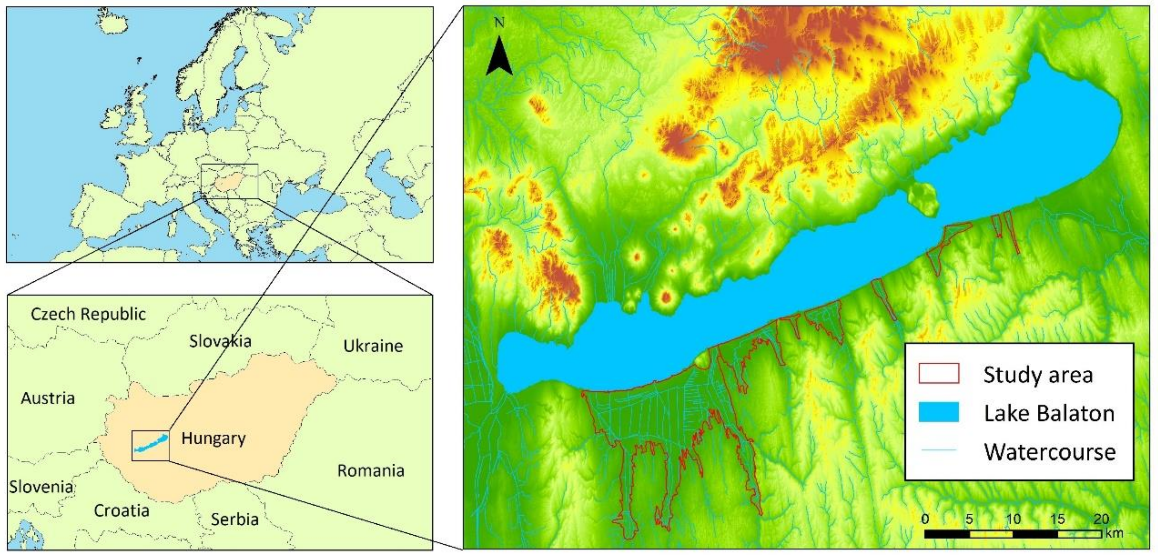
2.1. Study Area

Our study area is located along the southern shore of Lake Balaton, the largest lake in Central Europe. It forms a strip narrowing from west to east with an area of 194.8 km2. The marshes studied (Nagyberek, Ordacsehi-berek, Úszói-berek, Lellei-berek, Őszödi-berek, Földvári-berek, Szántódi-berek, Tóközi-berek and Töreki-berek) belong to the “Nagyberek” and “Somogy lakeshore plain” microregions [8,11] (Figure 1). The areas were selected from the map of the Second Military Survey [12], which still shows them in close-to-natural conditions and the geometrical accuracy allows comparisons with maps from later dates. The borders of marshes were identified on the basis of the representation of topography by striping and the location of the legend category ‘wet grassland’.
In the geology of the region, Middle to Late Miocene (‘Pannonian’) marine and lacustrine sediments with thicknesses of several hundreds of metres are dominant. As a consequence of tectonic processes leading to the formation of the Lake Balaton basin, a depression took shape in the late Middle Pleistocene. However, at first no contiguous water surface existed but ridges separated the partial lake basins which only merged 15–16 ka ago [13]. The lagoons were cut off from the main water body by sandy barrier bars accumulated by the prevailing northern and northwestern winds. An anoxyc environment of stagnant water was created where peat bog formation began [14].
The surface of the Balaton marshes is mostly flat. Marked landforms are the low ridges of former barrier bars [11]. In the topography of the study area, ridges which border the Nagyberek and the Ordacsehi-berek are still distinct.
In terms of climate, the western marshes are of the moderately warm and moderately wet climate type and at the eastern end, they are of moderately warm and moderately dry type. Annual mean temperature was 10.4 °C for the period 1961–1990. Long-term annual average precipitation reduces from west (670 mm) to east 620 mm [11].
The Lake Balaton and Sió River catchment is the largest independent hydrological unit in the western half of Hungary (Transdanubia) [15]. Drainage density is high, a number of small watercourses cross the marsh zone. The former swamps and bogs were drained and the water level of the lake was lowered but a considerable part of the marshes is still under the mean lakewater level. Continuous pumping and the maintenance of canals are indispensable to ensure agricultural cultivation. In the Nagyberek, a ca. 160 km-long network of canals serves the drainage of excess water [16]. The checkerboard pattern of canal network is clearly observable. The abundant standing waters are almost exclusively artificial structures, reservoirs and anglers’ lakes. A larger water surface of natural origin is only found in the Fehérvíz bog.
The local biota has only been preserved in patches. Most of the marshes are under cultivation but in the abandoned lands, moist grasslands and high forb vegetation are widespread [17], with many invasive species. Land drainage made forestry possible but it focused on species alien to the landscape (e.g., hybrid poplars). The most typical plant associations of wetland habitats are reed-beds, tussocks, swamp saw-grass and moist meadows. Fluctuations in groundwater level induced soil alkalization locally [11]. Native arboreous habitats include willow and alder bogs as well as oak-ash-elm groves, although the latter have been reduced to minimum extension. The marshes are valuable habitats for amphibians, reptiles and fishes, including the Common Toad (Bufo bufo), the European Pond Turtle (Emys orbicularis), the Corn Crake (Crex crex) [17], and in the Pogányvölgy meadows, an ice-age relict subspecies, the Central European Tundra Vole (Microtus oeconomus mehelyi) [18]. Remnants of the native fish fauna are represented by the European Bitterling (Rhodeus amarus), the Weatherfish (Misgurnus fossilis) and the European Mudminnow (Umbra krameri) [19]. The Balkanic subspecies of a venomous snake, specially protected in Hungary, the Bosnian Adder (Vipera berus bosniensis) is also found in the marshes [20]. The rich avifauna includes the White-tailed Eagle (Haliaeetus albicilla), the pretected bird with the highest nature conservation value [21], the Ferruginous Duck (Aythya nyroca) and the Black Stork (Ciconia nigra) is [22]. After land drainage, the plantation of small forest patches and the expansion of agricultural fields led to the appearance of the hunted game of the neighbouring hills, like the Red Deer (Cervus elaphus) and the Roe Deer (Capreolus capreolus) [23].

2.2. Methods to Study Land Use/Land Cover Change

Changes in land use were analyzed on maps prepared on seven dates. Past conditions were reconstructed from the maps of the First Military Survey (1783–1784, scale: 1:28,800) [24], Second Military Survey (1852–1857, 1:28,800) [12], Third Military Survey (1880–1882, 1:25,000) [25], the Military Survey of 1941 (1:25,000) [26], that of 1950–1952 (1:25,000) [27] and the topographic map from 1980 to 1989 (1:10,000) [28]. Present land use derives from the CORINE vector data base (2018) [29]. The original legend of CORINE was used in a modified form in order to adjust to the classes identified during research design (Table 1; columns 1 and 2).
For the processing of raster data, georeferencing was needed in some cases (e.g., for the maps of the 1941 [26] and 1950–1952 military surveys [27]). This operation was carried out by QGIS v3.4 software, the GDAL georeferencing module. Helmert transformation and linear resampling were employed. As a target projection the Uniform National Projection System (EPSG: 23,700) was set. Raster maps were digitized in ArcGIS environment using visual interpretation and ArcMap v10.8 and ArcGIS Pro 2.5 softwares. Altogether, nine land cover classes were identified for the study: wetland; grassland; arable land; water surface; vineyard, garden, orchard; built-up area; forest; mine; scrub. Map generalization was required to solve problems arising from the use of maps with different scales. The lowest-scale maps (poorest in information, 1:28,800) were those of the First and Second Military Surveys, to which the vectorized patches from more detailed maps were adjusted. For generalization, the guidelines of the European Environment Agency (EEA) prepared for the vecorization and generalization of CORINE Land Cover (CLC) classes [30] were used. When necessary, the following operations were made on large-scale maps: aggregation, amalgamation, classification, merging, selection, simplification [31,32]. Our experience was that on maps with a 1:28,800 scale, the size of the smallest vectorizable patches is c. 0.25 hectare. Therefore, the threshold suggested in the EEA guidelines was modified accordingly (spatial requirements: CLC/100, distance requirements: CLC/10). On 1:25,000-scale maps, minimal alterations were necessary. The smaller patches on large-scale (1:10,000) maps were merged to ensure similar richness of detail (Table 1; column 3).
Table 1. Correlation of the CORINE nomenclature [33] with our land use types and the generalization methods employed.
CORINE NomenclatureOur Land Use TypesMap Generalization Method to Ensure Similar Richness of Detail
4.1.1. Inland marshesWetlandamalgamation, merging, selection
Sample and description: [30] pp. 105–107. Modification of CLC nomenclature guidelines: minimum area is 0.25 hectare
2.3.1. Pastures
2.4.3. Land principally occupied by agriculture, with
significant areas of natural vegetation
3.2.1. Natural grasslands
Grasslandamalgamation, merging, selection
Sample and description: [30] pp. 52–64, and 75–81. Modification of CLC nomenclature guidelines: minimum area is 0.25 hectare
2.1.1. Non-irrigated arable landArable landamalgamation, merging
Sample and description: [30] pp. 39–42. Modification of CLC nomenclature guidelines: minimum area is 0.25 hectare
5.1.2. Water bodiesWater surfaceamalgamation, merging, selection
Sample and description: [30] pp. 116–119. Modification of CLC nomenclature guidelines: minimum area is 0.25 hectare
2.2.1. Vineyards
2.2.2. Fruit trees and berry plantations
2.4.2. Complex cultivation patterns
Vineyard, garden, orchardamalgamation, classification, merging, selection, simplification
Sample and description: [30] pp. 45–50. and 59–61. Modification of CLC nomenclature guidelines: minimum area is 0.25 hectare; distance for merging: 30 m.
1.1.2. Discontinuous urban fabric
1.2.1. Industrial or commercial units
1.2.2. Road and rail networks and associated land
1.4.2. Sport and leisure facilities
Built-up areaaggregation, amalgamation, merging, selection
Sample and description: [30] pp. 10–23. and 35–37. Modification of CLC nomenclature guidelines: minimum area is 0.25 hectare
3.1.1. Broad-leaved forest
3.1.3. Mixed forest
Forestaggregation, amalgamation, classification, merging, selection, simplification
Sample and description: [30] pp. 69–75. Modification of CLC nomenclature guidelines: minimum area is 0.25 hectare; distance for merging: 30 m
3.2.4. Transitional woodland-shrubScrubaggregation, amalgamation, classification, merging, selection, simplification
Sample and description: [30] pp. 87–92. Modification of CLC nomenclature guidelines: minimum area is 0.25 hectare; distance for merging: 30 m
The resolution of CORINE (smallest area represented: 25 ha) was not appropriate for the analysis of landscape units of small size. To remedy this deficiency, the original dataset was modified with satellite image (Sentinel–2 imageries for 9 September 2020, resolution: 10 m) [34,35]. Our primary goal was to represent on the map minor patches of wood, tree stripes, which are common landscape elements in the study area. Satellite images are widely applied tools for automatic forest classification [36]. For the classification bands 3 (green), 4 (red), 8 (near infrared) were used in 843 RGB band combination. Thus, vegetation appeared in red hues which allowed the sepration of patches. Learning areas were identifed to separate forests from other land cover classes. Classification was based on the maximum likelihood tool.
The confusion matrix (Table 2) created from the pixel statistics of the training areas shows that the accuracy of classification for forests was 94.1%, while 5.7% of the forests were classified as arable land and grassland. This inaccuracy, however, is not considerable. With the exception of built-up areas (not relevant for our research) all classes could be identified with a high accuracy.
The achieved raster dataset shows minor wooded patches too, but the picture is so rich in detail that generalization through an ArcMap Majority filter was needed. Boundaries between units were smoothed by the Boundary clean tool. The generalized dataset was then converted into a vector map and further refined through identifying patches smaller than 1000 m2. For the forest patches smaller than 0.25 hectare, the above described approaches of generalization were employed. The thus received polygons were intersected with a CLC 2018 map using the Intersect function to create a new field and to fill it with data using the Field calculator. If a patch did not appear as forest on the CORINE map but was identified as one in our dataset, the latter was accepted as reality. In all other classes, the original identification was retained. The resulting vector dataset seemed to be suitable for geometrical calculations (landscape metrics). The attribute table of the coverage was exported into xls fomat and using the Microsoft Excel table management program, the percentages of classes were computed for the study area and represented in diagrams.

2.3. Methods to Study Landscape Pattern Change

The analyses of functional landscape pattern are based on the patch-corridor-matrix model [37]. Areal units distinct from their environs by biophysical properties (geology, topography, hydrography, microclimate, soil and vegetation) are identified as patches. The dominant patch with the largest extension into which smaller patches are embedded is called the matrix [38]. Corridors are linear objects which ensure connectivity between patches. Their land use is variable, usually forest strips, wetlands or grassed strips [39]. Since all the three landscape components appear in vector databases as polygons (i.e., patches), they cannot be separated automatically by GIS tools. The geometrical properties (area, perimeter, shape etc.) and relative positions (proximity, connectivity etc.) of patches have to be computed to identify their character [40,41].
For landscape metrics, the ArcGIS vLATE module [42], a freely accessible tool of vector-based processing, is used. The details of the methodology applied is described and the table of indices is shown in [43], relying on [44,45,46,47,48,49]. Areal, perimeter, neighbourhood and diversity indices were involved into the analyses.
The following landscape-level indices were used:
  • TE (Total Edge): the total length of edges in a given patch type or landscape; suitable for landscape history analyses: for patches of similar sizes heterogeneity increases with growing TE.
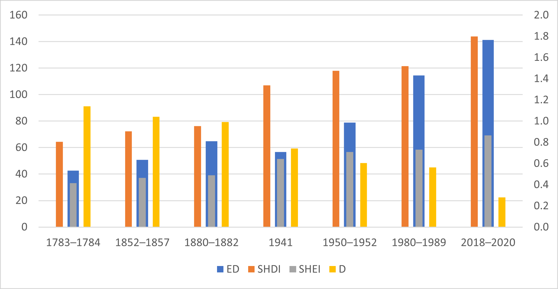
  • ED (Edge Density): length of edges per unit area; allows the comparison of landscapes of different sizes or the degree of fragmentation of patches.
  • NP (Number of Patches): total number of patches of the same type or within a landscape; a component of more complex indicators for landscapes of similar sizes or for historical evolution but no information of area, density or distribution.
  • SHDI (Shannon’s Diversity Index): richness of patches; high SHDI means the proportional distribution of patches, if there is only one patch, SHDI is 0.
  • SHEI (Shannon’s Evenness Index): shows the uniformity of patch type distribution; if one patch dominates, SHEI is close to 0, if there is only one patch, SHDI is 0.
  • D (Dominance): one or more patch type dominates in an area; complements SHEI as values close to 0 mean maximum evenness.
Patch-class-level indices:
  • TE (Total Edge) and NP (Number of Patches): see above.
  • MPE (Mean Patch Edge): medium size of a given patch class (what is the average edge length of patches); more complex than TE as considers NP too.
  • CA (Class Area): total area of the patch class; informs about landscape pattern, how prominent a patch type is in the landscape.
  • MPS (Mean Patch Size): average size for patches in one class; indicates landscape heterogeneity and allows comparisons among landscapes.
  • PSSD (Patch Size Standard Deviation): changes with MPS and patch size; indicates the variability of patch size.
  • DIVISION: based on cumulative distribution, shows the probability that two randomly selected points lie within different patches; it is 0 if there is only one patch; correlates negatively with MESH.
  • SPLIT (Splitting Index): also based on cumulative distribution, correlated with DIVISION; if there is only one patch, it is 1; the more the patches, the higher the value;
  • MESH (Effective Mesh Size): based on cumulative distribution, the higher its value, the more probable it is that two randomly selected points are within one patch; depends on the distribution of patch sizes and the proportion of the patch class within the landscape unit.
The different scales of the maps used and the intersection of the CORINE map with a raster coverage distorts the results to some extent. The grid of previous pixels is striking locally and, therefore, indices like the length of edges are not accurate. Such errors were corrected by generalization and inaccuracy was reduced to the minimum.

3. Results and Discussion

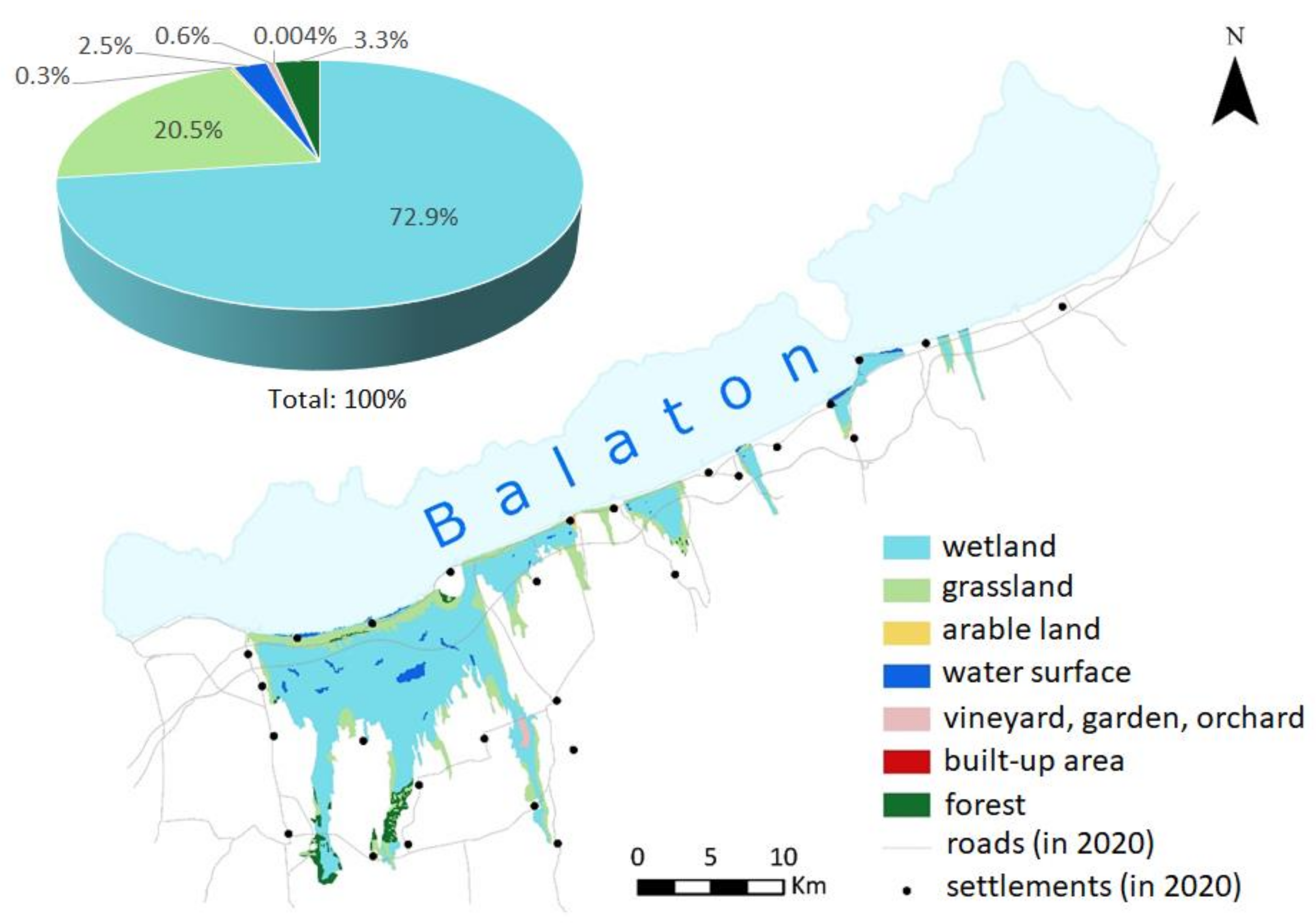
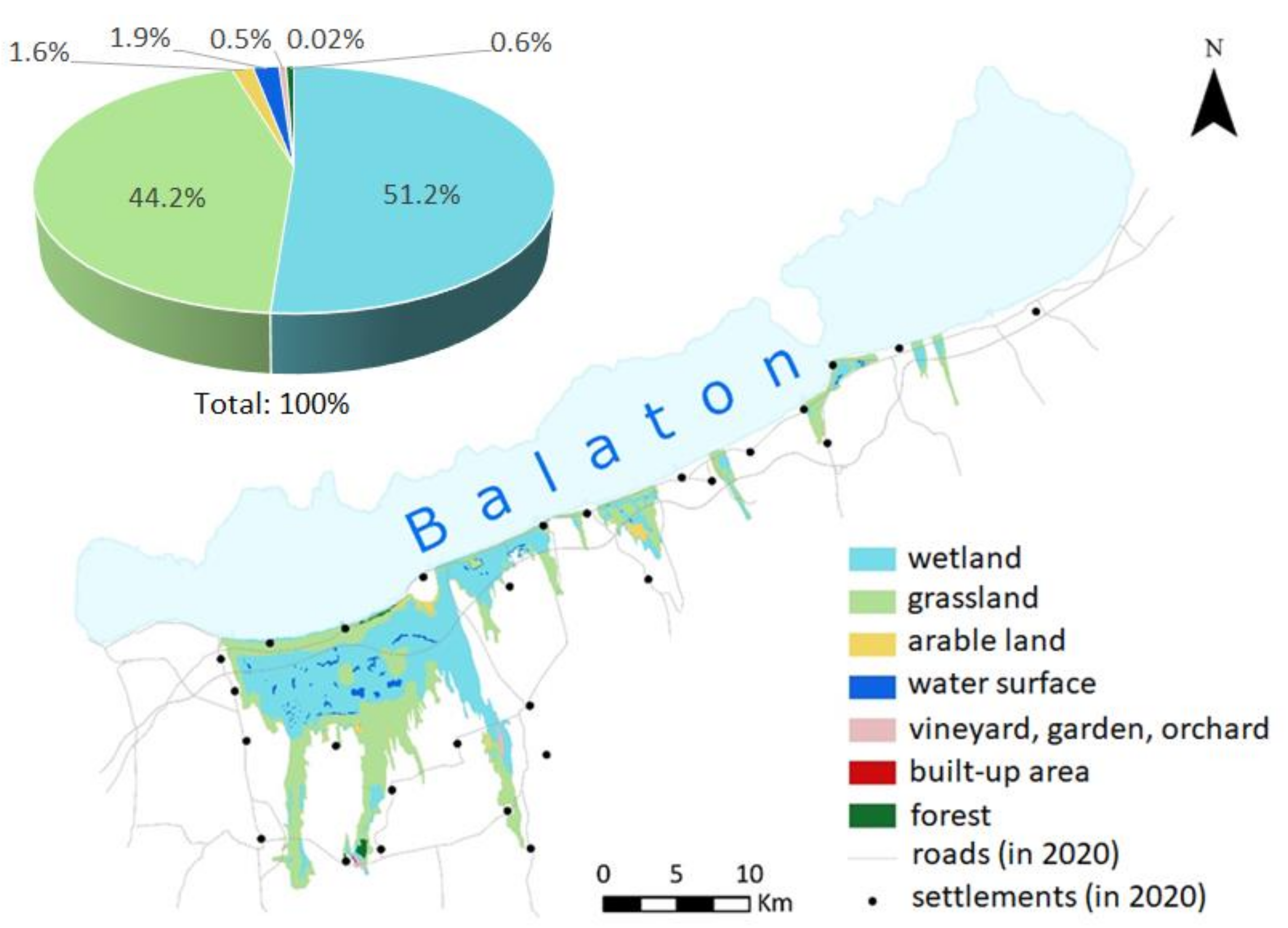
3.1. Land Use at the Time of the First Military Survey (1783–1784)

On the land use map of the First Military Survey [24] (Figure 2) wetlands (72.9%) clearly dominate. Open water surfaces covered 2.5% of the area. After the Battle of Mohács (1526) lost against the Ottomans, local population blocked the Sió Valley for strategic reasons, resulting in a considerable rise in the water level of Lake Balaton and inundating the marshes nearby [15]. Built-up areas were insignificant (0.003%) as population density was low. Farming only affected the higher-lying margins of marshes. Arable land only occupied 0.3% of the surface, while grasslands amounted to one-fifth (20.3%) of the area. Forested areas were present at 3.3%. The hydromorphic soils of lower areas were not suitable for vineyards, gardens or orchards; therefore, this class (0.6%) was restricted to the higher-lying grounds.

3.2. Landscape Pattern at the Time of the First Military Survey (1783–1784)

The predominance of wetlands in the 18th century defines this category as matrix. The value of total edge length (TE) is 831,730 m and edge density (ED) was only 42.7 m ha−1, which indicates a minimally fragmented landscape. Medium patch size was 5264 m2 and the total number of patches (NP) was 158. Shannon’s Diversity Index (SHDI) amounted to 0.806, while Shannon’s Evenness Index (SHEI) was 0.414. A low differentiation of the landscape pattern is observable. Dominance (D) had a value of 1.140, which means that a single patch type (wetlands) dominated landscape character.
In the interpretation of metric indices of patch classification, built-up areas were disregarded. (Only a single patch represented that class on the map.) The largest total edge length was represented by grasslands, while wetlands had a medium edge length (Table 3). This means that the latter had units low in number but, on average, higher in perimeter. Wetlands showed extremely high medium patch size (MPS) and patch size standard deviation (PSSD) values. Thus, wetland patches were usually quite large but, along with the large units, smaller ones also occurred. As far as neighbour indices are concerned, values of DIVISION and SPLIT indicate that grassland areas were the most dissected. Results of the MESH index again confirm the large size of wetlands. In this period, physico-geographical conditions, favourable over most of the study area, fully controlled the distribution of wetlands.

3.3. Land Use at the Time of the Second Military Survey (1852–1857)

Land use in the marshes had changed fundamentally by the time of the Second Survey (Figure 3). Most conspicuous on the map is the shrinkage of wetlands (to 51.2%). There are several explanations for this. In 1821, the watermill of Siófok burnt down and was not rebuilt. It ceased to impound water and led to a lower lakewater level [15]. At that time, an extensive network of canals conducted water from the marshland to Lake Balaton. In the 1850s, a drier spell started and also for railway construction lake level was lowered to reach its plummet in 1862 [50]. In 1863, the Sió sluice was inaugurated to allow water release from the lake [15]. The proportion of open water surfaces in the marsh was reduced to 1.9%. Grasslands expanded to 44.2% at the expense of wetlands, while arable land slightly grew to 1.9%. Vineyards, gardens and orchards stagnated (0.5%). Built-up areas did not surpass 0.02% and forests 0.6%. Woodlands used to be protected from commercial forestry by their inaccessibility due to the encircling wetlands. However, 19th-century drainage works exposed the latter as dry lands where, although with some delay compared to the neighbouring hills, intensive deforestation could begin.

3.4. Landscape Pattern at the Time of the Second Military Survey (1852–1857)

At the time of the Second Survey, human impact on the landscape pattern became clearly visible. The TE index increased to 986,732 m, ED to 50.66 m ha−1, NP to 187, while the average edge length remained stagnant (5276.64 m). Both SHDI (0.903) and SHEI (0.464) showed increases. Dominance dropped to 1.042. From all these, it can be concluded that landscape pattern diversified without a decisive class in land use.
In class-level analyses the low number and proportion of patches prevented us from considering built-up areas. Perimeter indices showed that in addition to the total length of edges, for medium length of edges, grasslands were in a leading position (Table 4). If both values are high, there are larger contiguous, less fragmented patches in this class. For areal indices, wetlands still showed the highest values but a decrease from the previous date was observed. On the other hand, grasslands had expanded and the structure of both classes had gotten closer to each other. The values of the neighbourhood indices DIVISON and SPLIT are closely correlated. Wetlands were the most uniform category and based on the efficient mesh size (MESH), they were organized into the largest contiguous areas.

3.5. Land Use at the Time of the Third Military Survey (1880–1882)

By the time of the Third Survey [25] the direction of changes had turned to its opposite (Figure 4). The area of wetlands was almost the same as in the 19th century (66.9%). In parallel, the proportion of open water surfaces increased to 2.7% in the 1871–1883 wet period [15]. Grassland areas shrank considerably (22.4%), while arable land expanded to occupy 6.6% of total area. No change occurred in the vineyard, garden, orchard class (0.4%). Built-up areas had slightly grown (0.2%). Forest area had expanded to 0.8% of the total area.

3.6. Landscape Pattern at the Time of the Third Military Survey (1880–1882)

Moreover, in landscape, pattern changes had been profound by the 1870s (Table 5). NP grew to 306 units and, consequently, TE increased to 1,261,357 m and ED to 64.75 m ha−1, while MPE was reduced (4123 m), probably due to the presence of more small patches with more complicated planform shapes. Slight rises can be observed for SHDI (0.954) and SHEI (0.490) and dominance (0.992) kept on decreasing.
Both total and medium edge length were found to be highest for wetlands. Medium edge length showed a moderate and TE a remarkable increase, i.e., patches became less compact as on the maps of the First Military Survey [24]. Although there is high similarity for the proportions of land use, landscape pattern were altered to a large extent over a century. Areal indices point to the preserved leading role of wetlands in MPS and PSSD. The growth of proportion of classes was bound to the increase of average patch size and its standard deviation. For grasslands, however, there was a drop in both metrics. Studying fragmentation, wetlands seemed to be the most uniform. The MESH index proves that they were arranged in the largest contiguous units, confirmed by DIVISION and SPLIT index values.

3.7. Land Use in 1941

The changes on the map of the 1941 military survey [26] are striking. Instead of wetlands, grasslands were predominant in the landscape and occupied one half of the study area (Figure 5). The share of arable land had reached 19.1% by 1941. A new water management concept was introduced: water bodies within the marshes were separated from those outside the marshes. The watercourses draining the Somogy Hills were collected by the newly built 17-km-long Western Canal in the Nagyberek [15]. Water surfaces showed no change in area (2.4%). Vineyards were planted in the zone between Fonyód and Balatonkeresztúr and their proportion (together with gardens and orchards) expanded to reach 3.4%. Vineyards on the northern shore had been destroyed by the phylloxery (root louse) epidemic but plantations on the sandy soils of the southern shore survived. Previous farmlands close to the lakeshore were developed and built-up areas amounted to 3.7% of total area. As water levels were dropping, peat extraction became possible for local use as fuel [16]. Peat pits covered 0.3% of the area in 1941. A negative development was the almost complete disappearance of forests (0.04%).

3.8. Landscape Pattern in 1941

The number of patches (229) and edge density (56.6 m ha−1) showed a slight decline compared to the previous date (Table 6). This can be explained by the expansion of grasslands and the formation of compact patches of arable fields with low specific edge length in the centre of the Nagyberek. Total edge length had been reduced to 1,103,061 m, while medium edge length had grown to 4,816.86 m. Among diversity indices, SHDI (1.338) and SHEI (0.643) continued the former increasing trend. Dominance (0.742) was reduced in comparison with the 19th century conditions.
Similarly to the Second Military Survey [12], perimeter indices were highest for grasslands. Along with a minor reduction of total edge length, medium edge length showed a considerable rise, patches were rearranged into larger units than before. The reason behind this is the conversion of reed-beds in the drained areas into grazing lands and meadows. This transformation had a great impact on landscape pattern. Class-level perimeter indices are controlled by grasslands with the same trend of change. Areal indices clearly confirm that landscape structure was dominated by grasslands, with outstanding values of CA, MPS and PSSD.
The analysis of the neighbourhood indices of DIVISION and SPLIT the class vineyards, gardens and orchards was the most uniform. In MESH, however, the areas of the individual classes are more influential and show that grasslands were merged into the largest contiguous units.

3.9. Land Use at the Time of the 1950–1952 Military Survey

In the early 1950s, the expansion of arable land continued and amounted to one-fourth of the marshes (25.6%), mostly in the central and western parts of the Nagyberek (Figure 6). The share of wetlands had slightly increased or remained unchanged. The extension of open water surfaces dropped to 1.5%. In 1949, the Balaton-Nagyberek State Farm was organized to develop arable farming. Drainage works continued and soil erosion problems arose since the desiccated muck is powdery and exposed to deflation by the northern winds which blow from the direction of Lake Balaton. To mitigate this situation the soils were rolled but this proved to be an only temporary solution. Finally, through planting forest strips, the problem could be eliminated [51]. Vineyards, gardens and orchards, replaced by housing developments, decreased to 2.3% and built-up areas occupied 4.7%. With more intensive peat extraction, mining areas (1%) showed an increase from the previous date. The reappearance of forests in the area was environmentally favourable. Their proportion grew to 2.7% over a single decade. The land use map represents numerous plots recently afforested probably with poplar varieties.

3.10. Landscape Pattern at the Time of the 1950–1952 Military Survey

By the early 1950s, the number of patches reached 503 and edge density 78.88 m ha−1 (Table 7). Both total and medium edge length values became higher, 1,536,546.7 m and 3054.76 m, respectively. The landscape turned more fragmented and more diverse (SHDI: 1.475, SHEI: 0.709 and dominance: 0.604.
Among perimeter indices, grasslands stood out with their total and medium edge length values. In the mid-20th century, this land use class remained prevalent but it lost in significance as a result of the expansion of arable land. The number of patches indicates that it was wetlands which became the most fragmented. Their area was about the same as at the previous date but they were divided into 122 more patches. The values of DIVISION and SPLIT were closely correlated. The most fragmented patches in this period were forests, while, as opposed to the previous date, arable fields and grasslands were the most uniform classes. As before, MESH was inversely proportional to the mentioned indices, grasslands having the highest and forests the lowest effective mesh size.

3.11. Land Use in the 1980s

In the land use of the 1980s, favourable and unfavourable tendencies can be equally discerned (Figure 7). A minor retreat of arable land (22.8%), and some expansion of grasslands (45.2%), open water surfaces (5.9%) and forests (9.2%) were observed. The proportion of wetlands fell below 10%, which adversely affected natural habitats. Further growth of built-up areas (5.9%) was characteristic due to touristic development and to the establishment animal ranches. In the state farm, arable farming had been gradually pushed to the back and was replaced by animal husbandry. The expansion of wooded areas was due to the planting of poplar varieties and forest strips. These processes led to a mosaical pattern which favoured the spreading of small and big game and created ideal conditions for game management [23]. The importance of fishery also increased and each marshland section had a fish pond. Vineyards, gardens and orchards declined to only 0.3% in the course of housing developments. Peat pits virtually disappeared (0.1%).

3.12. Landscape Pattern in the 1980s

No new trend was observed in landscape-level indices in the 1980s. The number of patches and edge density increased further, total and medium edge length maintained their inverse relationship, the former grew and the latter diminished (Table 8). Slight increases in Shannon diversity and evenness continued with dropping dominance.
In areal indices, grasslands had preserved their leading role. It is important to point out the inverse relationship between the dynamics of total and medium edge length. With the increasing share of grasslands, TE had also grown but MPE had been reduced. This means that another class (in this case, forests) fragmented the previously contiguous areas. In areal indices, patch number, total area of patches, average patch size and its standard deviation, the decisive role of grasslands was unambiguous. There were 318 forest patches which included agricultural shelter belts and sporadic wooded spots too. Their extension roughly equalled with that of built-up areas but their distribution was much more sporadic. In the 1980s, the DIVISION and SPLIT indices showed that built-up areas were the most uniform patches. For MESH, grasslands remained the leading class; they were arranged into the largest contiguous units but, in comparison with previous dates, with a considerably smaller mesh size.

3.13. Land Use Today (2018–2020)

The present land use is extremely heterogeneous but, all in all, the observed processes are favourable for the biota. The proportion of arable land has been reduced to 16.5% and wetlands show a major expansion (17.8%) (Figure 8). Open water surfaces have reached a share of 6.6%. Forested area occupies 15.8%, which is a highly positive development. For its evaluation, however, it has to be considered that to a large part forests include introduced or spontaneously spread invasive species. Bushes and scrubs make up 1.7%, habitats typically resulting from the mixing of alien and domestic species. The general trend of land use change is towards extensification. The numbers of grazed animals have substantially dropped and natural vegetation could not regenerate. Arable fields and grazed lands were partly abandoned and pioneer and invasive plants took ground. Artificial patches, mostly due to housing development, have extended to 11% of the marshes by now. Development focuses on the lakeshore and in the zone of national motorway M7.

3.14. Landscape Pattern Today (2018–2020)

By today, landscape-level indices have reached extreme values: the metrics with a decreasing trend over the previous centuries show extreme lows, while those with an increasing trend present maxima. The number of patches is 2083, edge density is 141.21 m ha−1, TE is 2,748,754 m, MPE is 1320 m, SHDI is 1.8 and SHEI 0.866 (Table 9). Dominance diminished to 0.279.
The indices for forests are particularly extreme and have the largest total edge length and the lowest medium edge length values. This situation results from the spontaneously developed sporadic wooded patches of irregular shape and from the introduction of agricultural shelter belts, which have long edges related to their size. This pattern, however, is partly due to the deficiency of our methodology which intersects classified high-resolution satellite data with the CORINE land cover map much poorer in detail. Among areal indices, grasslands still show high values, their extension is the largest and the standard deviation of patch size is 139.02 ha. On the other hand, MPS for open water surfaces is higher, which means larger units on the average with number of patches (127) lowest among all classes. Forest patches appear in the largest number (1383). DIVISION and SPLIT values indicate that forests are the most fragmented and built-up areas are the most uniform, which is due to their concentration on the lakeshore zone and along the motorway in homogeneous blocks. The highest MESH value is found for grasslands; they are dominant in the landscape and form the matrix.

3.15. Changes in Land Use Classes

The environment of the South-Balaton marshes has been fundamentally transformed over the past centuries, primarily through the shrinkage of wetlands, which was, however, not a continuous process (Figure 9). The map of the Third Military Survey shows that wetlands grew as a result of a more humid spell and in the last three decades, land use extensification generated their areal expansion again. In the first decades of the 20th century, they became classes of secondary importance compared to grasslands, which took over the leading role in land use in the 1940s.

3.16. Opportunities for Landscape Rehabilitation

Based on the quantitatively described and evaluated land use and landscape pattern as well as the ecological system of the study area proposals were formulated for the rehabilitation of the landscape (Figure 10). Naturally, the complete restoration of natural conditions is not possible but, adjusted to nature conservation efforts (such as the Natura 2000 network, Ramsar Convention), a close-to-nature vegetation can be a target of rehabilitation.
In transformed landscapes, traces of the original vegetation are often preserved on field margins or in small wooded patches [52]. In the case of the South-Balaton marshes it is typical along canals, in shelterbelts and in abandoned quarries–areas without disturbance for decades. Good examples for the preservation of native vegetation are the presence of the Marsh Helleborine (Epipactis palustris), the Sea Rush (Juncus maritimus), the Loose-flowered Orchid (Orchis laxiflora ssp. palustris), a Black Bog-Rush (Schoenus nigricans), the One-glumed Spikesedge (Eleocharis uniglumis) and the White Waterlily (Nymphaea alba), which are abundant in the area [53]. In the restoration it is crucial to focus on areas which are the last refuges of the above listed species. To this end, we propose that buffer zones, gallery forests, should be created along canals to ensure undisturbed habitats.
The main goal is to raise the level of ecosystem services. Provisioning ecosystem services in wetlands include the supply of water, food, timber, medicinal plants and genetic resources for plant breeding. Regulating services affect air, water and climate and cover erosion control, the prevention of natural disasters and diseases, water purification and pollination. Cultural services are related to landscape aesthetics, spiritual and religious values, resources for recreation and tourism, traditional farming (pastoral crafts, fishery, gathering wetland products etc.) as well as the inspiration for arts and architecture provided by the landscape. Supporting services refer to soil formation, photosynthesis, water and nutrient circulation and biodiversity. It is widely believed and even proven that to substitute all those services which are ensured by nature free of charge and on the long term by technological solutions would be extremely expensive. Quantifying the services, it is evident that the investment into ecosystem services bring return which is much higher than the necessary investment [54].
In our opinion, there is no need to change the already established regional groundwater table but to preserve wetlands water retention is required in selected areas through blocking some canals and providing them with locks. This way runoff can be slowed down and part of the sudden rainwater surge can be stored temporarily. To this end, further reservoirs are also proposed on the lower sections of the canals conducting water to Lake Balaton. Buffering and filtering functions are to be equally utilized. Sediment load and fertilizer and pesticide residues washed down from agricultural fields could settle in reservoirs of some hectare area, reducing pressure on the lake and improving water quality. Such a reservoir could be constructed for each marsh. In the densely built-up shore zone water fowl are exposed to heavy disturbance but water surfaces would ensure feeding ground and shelter for them and also enhance biodiversity. Along the canals, buffer zones also promote ecosystem services. In the shore belt, close-to-natural vegetation should spread under regulated conditions repressing alien species and thus encouraging numerous favourable processes. For aquatic associations, particularly for fish stocks, disturbance along the shore is of utmost importance. Soil erosion could also be mitigated and water surges would cause less removal of the loose sediments. More atmospheric carbon-dioxide could be bound in vegetation which is in line with climate protection goals [54].
In the changes of land use proportions, the shrinkage of arable land parallel with the spreading of wetlands, grasslands and forests is the most favourable development. The retreat of arable land has been going on for decades. Rational land use is the objective but the total elimination of this class is not desirable from an economic viewpoint. When preparing a habitat rehabilitation plan, we identified arable fields lying below the mean water level of Lake Balaton and in or near Natura 2000 areas. Land use can be optimized in such areas endangered by excess water through their conversion to grasslands employing grass mixtures. Thus, a transitional zone could be created between intensively used agricultural fields and protected areas, grassed patches could be made more compact, the edge effect would become minimal and the disturbance of habitats would be reduced. Grassland management is indispensable since unmanaged grasslands are prone to be infected by weeds and to degradation. Invasive arboreous and herb species have to be repressed through mowing and grazing carefully adjusted to the phenology of protected plant species. Information from farmers about preferred land management is necessary. The direction of mowing has to be planned and tractors should be supplied with shocking chains to alarm game. A kind of extensive use would be grazing by native domestic animals in optimal density, which could effectively prevent adventive species from spreading and increase soil organic matter content. Here, profitability is lower than in large-scale stock breeding but more sustainable and would allow the exploitation of the potential for ecotourism in the vicinity of Lake Balaton.
In the arable fields which remained environmentally acceptable, cultivation with reduced tillage and more effective preservation of soil organic matter would be optimal. Cutting up stalk residues and mixing them evenly with the topsoil would improve soil structure at a 15–25 m depth and absorb carbon in the form of humus [55].
We also propose the planting of gallery forests in the eastern part of the Nagyberek in a ca. 50–100 m wide, almost continuous strip along watercourses of south to north alignment. In addition to binding CO2 the effect on microclimate would also be favourable, increasing humidity and protecting the soil from desiccation through shading. They provide good habitats for amphibians, which could move unhindered between the Fehérvíz bog and the northern wetlands. Emphasis is laid on the application of native and resistent trees like willows, poplars, pedunculate oak and black alder. Afforestation and forest maintenance are financed from governmental sources.
Biodiversity as a supporting service requires regular management. In the southern Balaton marshes, there is only one legally protected area, the Fehérvíz Nature Reserve of the Nagyberek. However, 74% of the study area is part of the Natura 2000 network. The Ramsar Convention area “Fishponds and Marshlands South of Lake Balaton” includes the eastern and southern sections of the Nagyberek as well as the Ordacsehi, Úszó, Lelle, Őszöd, Földvár, Tóköz and Töreki marshes [56].
The management plans for Natura, 2000 areas focus on the repression of invasive plants, aim at the preservation of valuable plant associations and encourage sustainable farming, but mostly neglect the management of reed-beds, which are central for the conservation of wetland habitats. Considering physical geographical and ecological endowments, a detailed plan of reed economy should be prepared. In the 1940s, reed harvesting in winter was widespread and provided the local population with subsidiary income [57]. As the demand for reed as a raw material declined and wetlands shrank, this practice was abandoned and the quality of reed-beds deteriorated. Today modern agricultural technology could allow sustainable reed economy. Harvesting should be reduced to limited areas since for birds nesting in spring and early summer older, decayed and heterogeneous reed stands are indispensable [58].
The newly emerged plant species found in the study area in recent decades include Adonis vernalis, Crocus reticulatus, Orchis laxiflora ssp. palustris, Ranunculus lingua, Schoenus nigricans and Thelypteris palustris [53]. These species should receive special attention in planning marsh management to increase biodiversity.

4. Conclusions

In industrial countries, wetlands are retreating. Close-to-natural ecosystems are being replaced by agricultural fields, built-up areas or they survived in a more and more fragmented form. In Hungary, the southern Balaton marshes show transformation trends closest to those observed in the Fertő-Hanság National Park. In both regions, most intensive transformation occurred in the period from the Third Military Survey [25] to the present. Drainage reduced water levels in both Lake Balaton and Lake Fertő (Neusiedlersee), open water surface shrank and arable land expanded at the expense of wetlands and grasslands. In the Hanság, poplar varieties were extensively planted too [59]. In recent decades, however, favourable trends in land use are detected for both areas. Arable land of low fertility is increasingly abandoned and more natural vegetation is allowed to regenerate. In many cases, however, the spreading of invasive species hinders this process [60,61].
In addition to being valuable habitats, the marshes in the southern neighbourhood of Lake Balaton are also suitable to temporarily store surges of rainwater both on the surface and in the soil and, thus, fulfilling a buffering function. To intensify this function, large-scale rehabilitation would be necessary but complete landscape restoration would be cost-intensive and contradict the interests of farmers and local population. Partial rehabilitation, however, is feasible in areas of high nature conservation value. In this paper, proposals are made for the allocation of water retention structures and for modifications in land use. The final goal is the improvement of the provision level of ecosystem services which truly reflect the value of the landscape [50,51].
Investigating landscape changes in international comparison, it becomes clear that the same processes which affect wetlands operate at different rates. In the Doñana marshland of southern Spain, in 1918, over 99.8% of the area natural and close-to-natural ecosystems were found, while by 2006, their share dropped to 29.6%. In the Doñana intensive landscape change started later but was more rapid than in the wetlands of Hungary. In parallel with but belated by Hungarian developments, after the 1998 plummet, however, a modest growth of more natural habitats is observable [3].

Author Contributions

Conceptualization: P.G., D.L. and G.N.; methodology: G.N., P.G. and D.L.; software: G.N.; validation: P.G., D.L. and G.N.; writing (original draft preparation): G.N.; writing (review and editing): G.N., P.G. and D.L.; visualization: G.N.; supervision: D.L. and P.G. All authors have read and agreed to the published version of the manuscript.

Funding

This research received no external funding.

Institutional Review Board Statement

Not applicable.

Informed Consent Statement

Not applicable.

Data Availability Statement

Acknowledgments

The authors would like to acknowledge the Institute of Geography and Earth Sciences, Faculty of Sciences, University of Pécs for providing software and maps. Gergő Németh would like to thank the New National Excellence Programme of the Ministry for Innovation and Technology (code number: ÚNKP-21-3-I) for the professional support.

Conflicts of Interest

The authors declare no conflict of interest.

References

  1. Berényi, I. Kultúrtájváltozás a 18. században (Changes in cultural landscape in the 18th century). In A Kárpát-Medence Földrajza (Geography of the Carpathian Basin); Dövényi, Z., Ed.; Akadémiai Kiadó: Budapest, Hungary, 2012; pp. 386–389. [Google Scholar]
  2. Burton, T.M.; Uzarski, D.G. Marshes-Non-wooded Wetlands. In Encyclopedia of Inland Waters; Elsevier: Amsterdam, The Netherlands; Boston, MA, USA, 2009; pp. 531–540. ISBN 978-0-12-370626-3. [Google Scholar]
  3. Zorrilla-Miras, P.; Palomo, I.; Gómez-Baggethun, E.; Martín-López, B.; Lomas, P.L.; Montes, C. Effects of Land-Use Change on Wetland Ecosystem Services: A Case Study in the Doñana Marshes (SW Spain). Landsc. Urban Plan. 2014, 122, 160–174. [Google Scholar] [CrossRef]
  4. Turner, M.G.; Gardner, R.H. Landscape Ecology in Theory and Practice; Springer: New York, NY, USA, 2015; ISBN 978-1-4939-2793-7. [Google Scholar]
  5. McGarigal, K. Landscape pattern metrics. In Encyclopedia of Environmetrics; Abdel, H.E.-S., Walter, W.P., Eds.; John Wiley & Sons: Chichester, UK, 2002; pp. 1135–1142. [Google Scholar]
  6. Riitters, K. Pattern Metrics for a Transdisciplinary Landscape Ecology. Landsc. Ecol. 2019, 34, 2057–2063. [Google Scholar] [CrossRef] [Green Version]
  7. Túri, Z. A Tájmintázat Vizsgálata a Tiszazugban (Landscape Pattern in the Tiszazug). Tájökológiai Lapok 2011, 9, 43–51. [Google Scholar]
  8. Csorba, P. Magyarország Kistájai (Microregions of Hungary); Meridián Táj- és Környezetföldrajzi Alapítvány: Debrecen, Hungary, 2021; ISBN 978-963-89712-4-1. [Google Scholar]
  9. Tarnawa, Á.; Pósa, B.; Kassai, K.; Nyárai, F.H.; Farkas, A.; Birkás, M.; Jolánkai, M. Climate Change Research Review–10th Anniversary of the VAHAVA Report. Columella 2017, 4, 55–62. [Google Scholar] [CrossRef]
  10. Nagy, G.; Lóczy, D.; Czigány, S.; Pirkhoffer, E.; Fábián, S.Á.; Ciglič, R.; Ferk, M. Soil Moisture Retention on Slopes under Different Agricultural Land Uses in Hilly Regions of Southern Transdanubia. HunGeoBull 2020, 69, 263–280. [Google Scholar] [CrossRef]
  11. Magyarország Kistájainak Katasztere (Inventory of the Microregions of Hungary), 2nd ed.; Dövényi, Z. (Ed.) MTA Földrajztudományi Kutatóintézet: Budapest, Hungary, 2010; ISBN 978-963-9545-29-8. [Google Scholar]
  12. Második Katonai Felmérés (Second Military Survey). Königreich Ungarn. Digitized Maps of the Habsburg Empire 1806–1869 (1:28800); DVD; Arcanum Adatbázis Kft: Budapest, Hungary, 2005. [Google Scholar]
  13. Mezősi, G. A Dunántúli-dombság nagyobb tájföldrajzi egységeinek genetikai vázlata és természetföldrajzának néhány kérdése (The origin and physical geography of major landscape units of the Transdanubian Hills). In Magyarország Természetföldrajza (Physical Geography of Hungary); Akadémiai Kiadó: Budapest, Hungary, 2011; pp. 299–304. [Google Scholar]
  14. Hahn, G. Magyarország Tőzeg- És Lápföldvagyona (Peat and Muck Reserves in Hungary). Földtani Kut. 1984, 27, 85–94. [Google Scholar]
  15. Károlyi, Z.; Vázsonyi, Á. A Balaton és vízrendszere (Lake Balaton and its drainage system). In A magyar Vízszabályozás Története (History of Water Regulation in Hungary); Ihrig, D., Ed.; Országos Vízügyi Hivatal: Budapest, Hungary, 1973; pp. 249–271. [Google Scholar]
  16. Dömsödi, J. Adatok a Nagyberek És Környéke Lápterületeinek Hasznosításához (Data on the Utilization of the Bogs in the Nagyberek and Its Environs). Agrokémia Talajt. 1976, 25, 115–130. [Google Scholar]
  17. Nagy, G.G. Nagyberek Természetföldrajza (Physical Geography of the Nagyberek), Budapesti Corvinus Egyetem, Tájépítészeti Kar; Tájtervezési és Területfejlesztési Tanszék: Budapest, Hungary, 2011. [Google Scholar]
  18. József, L.; György, R.; Gabriella, S.L. A Pogány-Völgyi Rétek Natura 2000 Terület Kisemlős Közösségeinek Vizsgálata, Különös Tekintettel Az Északi Pocok (Microtus Oeconomus) Előfordulására. Nat. Som. 2015, 27, 107–114. [Google Scholar] [CrossRef]
  19. Ferincz, Á.; Ádám, S.; András, W.; Sütő, S.; Soczó, G.; Ács, A.; Kováts, N.; Paulovits, G. Adatok a Dél-Balatoni Berekterületek Halfaunájához. Nat. Som. 2014, 24, 279–286. [Google Scholar]
  20. Magyarország Kételtűi És Hüllői: Keresztes Vipera. Available online: https://www.mme.hu/keteltuek-es-hullok/keresztes-vipera (accessed on 6 November 2021).
  21. Natura 2000-Standard Data form Balatoni Berkek. Available online: https://natura2000.eea.europa.eu/Natura2000/SDF.aspx?site=HUDD10012 (accessed on 6 November 2021).
  22. Kovács, G.; Jakus, L. A Tóközi-Berek (Zamárdi) Madártani Felmérése [The Ornithological Survey of the Tóközi-Berek (Marsh) at Zamárdi]. Nat. Som. 2015, 26, 117–122. [Google Scholar]
  23. Ancsin, G. Egy Elfeledett Ősmocsár–A Balatoni Nagy-Berek (A Forgotten Ancient Swamp, the Nagy-Berek of Lake Balaton). Available online: https://afoldgomb.hu/magazin/a-foldgomb-2019-tavaszi-kulonszam/egy-elfeledett-osmocsar-a-balatoni-nagy-berek (accessed on 15 September 2021).
  24. Első Katonai Felmérés (First Military Survey). Königreich Ungarn. Digitized Maps of the Habsburg Empire 1763–1785 (1:28,800), DVD.; Arcanum Adatbázis Kft: Budapest, Hungary, 2004. [Google Scholar]
  25. Harmadik Katonai Felmérés (Third Military Survey). Königreich Ungarn. Digitized Maps of the Habsburg Empire 1869–1887 (1:25000), DVD.; Arcanum Adatbázis Kft: Budapest, Hungary, 2007. [Google Scholar]
  26. Magyarország Katonai Felmérése 1941 (Military Survey of Hungary in 1941), (1:25,000); HM Hadtörténeti Intézet És Múzeum Térképtára: Budapest, Hungary, 1941.
  27. A Magyar Néphadsereg 1951-Ben Helyesbített, 1952-Ben Kiadott Térképszelvényei (Map Sections Created by Hungarian People’s Army, Corrected in 1951, Published in 1952), (1:25,000); (Hungarian People’s Army): Budapest, Hungary.
  28. Magyarország EOTR Topográfiai Felmérése 1980–1989 (EOTR Topographic Survey of Hungary 1980–1989) (1:10000); Mezőgazdasági És Élelmezésügyi Minisztérium: Budapest, Hungary, 1989.
  29. European Environment Agency Corine Land Cover (CLC). 2018. Available online: https://land.copernicus.eu/pan-european/corine-land-cover/clc2018 (accessed on 16 August 2021).
  30. Kosztra, B.; Büttner, G.; Hazeu, G.; Arnold, S. Updated CLC Illustrated Nomenclature Guidelines 2019; European Environment Agency: Wien, Austria, 2017; pp. 1–24. [Google Scholar]
  31. Shea, K.S.; Master, R.B.M. Cartographic Generalization in a Digital Environment: When and How to Generalize; American Society for Photogrammetry and Remote Sensing and American Congress on Surveying and Mapping: Falls Church, VA, USA, 1989; pp. 56–67. [Google Scholar]
  32. Susetyo, D.B.; Hidayat, F. Specification of Map Generalization from Large Scale to Small Scale Based on Existing Data. IOP Conf. Ser. Earth Environ. Sci. 2019, 280. [Google Scholar] [CrossRef]
  33. CLC Nomenclature Guidelines. Available online: https://land.copernicus.eu/user-corner/technical-library/corine-land-cover-nomenclature-guidelines/html (accessed on 20 September 2021).
  34. Copernicus Open Access Hub-Sentinel-2 Image. Available online: https://scihub.copernicus.eu/dhus/odata/v1/Products(’0d47cb1c-a1b1-4e5b-bc79-2f4fcd91115f’)/$value (accessed on 16 August 2021).
  35. Copernicus Open Access Hub-Sentinel-2 Image. Available online: https://scihub.copernicus.eu/dhus/odata/v1/Products(’91c6b176-412a-4581-af4f-c76ff64133aa’)/$value (accessed on 17 August 2021).
  36. Szabó, L.; Deák, M.; Szabó, S. Comparative Analysis of Landsat TM, ETM+, OLI and EO-1 ALI Satellite Images at the Tisza-Tó Area, Hungary. Landsc. Environ. 2016, 10, 53–62. [Google Scholar] [CrossRef]
  37. Forman, R.T.T.; Godron, M. Landscape Ecology; John Wiley and Sons: New York, NY, USA, 1986; ISBN 978-0-471-87037-1. [Google Scholar]
  38. Kerényi, A. Tájvédelem (Landscape Protection); Pedellus Tankönyvkiadó: Debrecen, Hungary, 2007; ISBN 978-963-9612-54-9. [Google Scholar]
  39. Csorba, P.; Horváth, G.; Mezősi, G.; Lóczy, D.; Mucsi, L.; Szabó, M. Geoökológiai Alapú Tájtervezés Elméleti És Gyakorlati Kérdései (Theory and Practice of Geoecological Landscape Planning); Szegedi Tudományegyetem: Szeged, Hungary, 2013. [Google Scholar]
  40. Szabó, S. Tájmetriai Mérőszámok Alkalmazási Lehetőségeinek Vizsgálata a Tájanalízisben (Opportunities for the Application of Landscape Indices in Landscape Analysis). Ph.D. Thesis, Debreceni Egyetem Természettudományi és Technológiai Kar, Debrecen, Hungary, 2009. [Google Scholar]
  41. Csorba, P.; Szabó, S. The Application of Landscape Indices in Landscape Ecology. In Perspectives on Nature Conservation-Patterns, Pressures and Prospects; Tiefenbacher, J., Ed.; InTech: London, UK, 2012. [Google Scholar]
  42. Vector-Based Landscape Analysis Tools (Extension for ArcGIS 10.8): V-LATE 2.0 (Programming: Dirk Tiede). Available online: https://hub.arcgis.com/content/69963ab422d04e649b64ac11cbadafed/about (accessed on 16 August 2021).
  43. Túri, Z. A Tájszerkezet Geoinformatikai Módszereinek Elemzése Alföldi Mintaterületen (Landscape Pattern Analysis by GIS in a Lowland Area); Debreceni Egyetem Természettudományi Doktori Tanács Földtudományok Doktori Iskola: Debrecen, Hungary, 2015. [Google Scholar]
  44. O’Neill, R.V.; Krummel, J.R.; Gardner, R.H.; Sugihara, G.; Jackson, B.; DeAngelis, D.L.; Milne, B.T.; Turner, M.G.; Zygmunt, B.; Christensen, S.W.; et al. Indices of Landscape Pattern. Landsc. Ecol. 1988, 1, 153–162. [Google Scholar] [CrossRef]
  45. McGarigal, K.; Marks, B.J. FRAGSTATS: Spatial Pattern Analysis Program for Quantifying Landscape Structure; U.S. Department of Agriculture, Forest Service, Pacific Northwest Research Station: Portland, OR, USA, 1995; p. PNW-GTR-351. [Google Scholar]
  46. Jaeger, J.A.G. Landscape Division, Splitting Index, and Effective Mesh Size: New Measures of Landscape Fragmentation. Landsc. Ecol. 2000, 15, 115–130. [Google Scholar] [CrossRef]
  47. IDEFIX—Integration Einer Indikatorendatenbank für Landscape Metrics in ArcGIS 8.x. Available online: http://www.agit.at/s_c/papers/2003/1645.pdf (accessed on 1 August 2021).
  48. Lang, S.; Tiede, D. vLATE Extension für ArcGIS–Vektorbasiertes Tool zur Quantitativen Landschaftsstrukturanalyse. Available online: https://uni-salzburg.elsevierpure.com/en/publications/vlate-extension-f%C3%BCr-arcgis-vektorbasiertes-tool-zur-quantitativen (accessed on 13 August 2021).
  49. McGarigal, K.; Marks, B.J. Fragstats. Available online: https://www.umass.edu/landeco/pubs/mcgarigal.marks.1995.pdf (accessed on 11 October 2021).
  50. Bendefy, L. A Balaton Vízszintjének Változásai a Neolitikumtól Napjainkig (Water Level Changes of Lake Balaton from the Neolithic to the Present Day). Hidrológiai Közlöny 1968, 48, 257–262. [Google Scholar]
  51. NAGY-BEREK Fehér-Vízi Láp (Nagy-Berek, Fehér-Víz Bog); Temesi, I. (Ed.) Tájak–Korok–Múzeumok Szervező Bizottsága és az Országos Környezet-és Természetvédelmi Hivatal: Budapest, Hungary, 1983; ISBN 963-555-186-X. [Google Scholar]
  52. Milberg, P.; Bergman, K.; Jonason, D.; Karlsson, J.; Westerberg, L. Forest Ecology and Management Land-Use History in Fl Uence the Vegetation in Coniferous Production Forests in Southern Sweden. For. Ecol. Manag. 2019, 440, 23–30. [Google Scholar] [CrossRef]
  53. Rozner, G.; Miókovics, E.; Vidéki, R. Védett Növényfajok Előfordulási Adatai Észak-Somogyban. Nat. Som. 2011, 19, 5–16. [Google Scholar]
  54. Everard, M.; Jevons, S. Ecosystem Services Assessment of Buffer Zone Installation on the Upper Bristol Avon, Wiltshire; Environment Agency: Bristol, UK, 2010; ISBN 978-1-84911-176-8. [Google Scholar]
  55. Szabó, I.; Balázsy, S.; Végső, Z.; Jens, M.; Vajda, P. A Forgatás Nélküli Mulcsos Talajművelés Mint a Tarlómaradványok Mikrobiális Lebontásának Leghatékonyabb Technológiája (Mulching without Ploughing as the Most Effective Technology for the Microbiological Decomposition of Stubble Residues). Környezetkímélő Talajművelési Rendszerek Magyarországon. Available online: http://www.mtafki.hu/konyvtar/kiadv/ktrm/pdf/010_Szabo.pdf (accessed on 7 May 2021).
  56. Ramsar Sites Information Service—Fishponds and Marshlands South of Lake Balaton. Available online: https://rsis.ramsar.org/ris/1963 (accessed on 16 September 2021).
  57. Friesz, K. Zamárdi a XX. században (Zamárdi in the 20th century). In ZAMÁRDI Községtörténeti Tanulmányok; Zamárdi nagyközség képviselő-testülete: Zamárdi, Hungary, 1997; ISBN 963-03-4296-0. [Google Scholar]
  58. Kozák, L. Élőhely-Kezelés (Habitat Management); Debreceni Egyetem. Agrár—és Gazdálkodástudományok Centruma: Debrecen, Hungary, 2011. [Google Scholar]
  59. Konkoly-Gyuró, É.; Tirászi, Á.; Balázs, P.; Nagy, D.; Király, G. A vízrendszer, a felszínborítás és a tájkarakter változása a Fertő-Hanság medencében (Changes of the watercourse system, land cover and landscape character in the Fertő-Hanság basin). In A táj Változásai a Kárpát-Medencében (Landscape Changes in the Carpathian Basin); Sopron, Hungary, 2014; pp. 42–48. Available online: http://www.emk.nyme.hu/fileadmin/dokumentumok/emk/evgi/TajTanszek/Publik%C3%A1ci%C3%B3k/Konkoly-Gyur%C3%B3_etal_V%C3%ADzrendszer_felsz%C3%ADnbor%C3%ADt%C3%A1s_Fert%C5%91_f.pdf (accessed on 8 August 2021).
  60. Molnár, Z.; Gergely, A. A Körtvélyes-Sziget Élőhely-Változásai (Habitat Changes of the Körtvélyes-Island). Tájokológiai Lapok 2008, 6, 333–341. [Google Scholar]
  61. Ujházy, N.; Bíró, M. A Vizes Élőhelyek Változásai Szabadszállás Határában (Changes of Wetlands on the Border of Szabadszállás). Tájökológiai Lapok 2013, 11, 291–310. [Google Scholar]
Figure 1. Location of study area.
Sustainability 13 12664 g001
Figure 2. Land use map at the time of the First Military Survey (1783–1784).
Sustainability 13 12664 g002
Figure 3. Land use map at the time of the Second Military Survey (1852–1857).
Sustainability 13 12664 g003
Figure 4. Land use map at the time of the Third Military Survey (1880–1882).
Sustainability 13 12664 g004
Figure 5. Land use map in 1941.
Sustainability 13 12664 g005
Figure 6. Land use map at the time of the 1950–1952 military survey.
Sustainability 13 12664 g006
Figure 7. Land use map in the 1980s.
Sustainability 13 12664 g007
Figure 8. Land use map today (2018–2020).
Sustainability 13 12664 g008
Figure 9. Changes in land use classes.
Sustainability 13 12664 g009
Figure 10. Opportunities for landscape rehabilitation.
Sustainability 13 12664 g010
Table 2. The confusion matrix of the classification of satellite images.
ForestArable Land and GrasslandWater SurfaceBuilt-up Area
Forest94.1%0.0%0%0%
Arable land and grassland5.7%99.8%0%50.3%
Water surface0.0%0.0%99.8%0%
Built-up area0.2%0.2%0.1%49.7%
Total100%100%100%100%
Bold numbers: Accuracy of the classified land use categories.
Table 3. Landscape metrics at the time of the First Military Survey (1783–1784).
ClassTE
(m)
MPE
(m)
NP
(pc)
CA
(ha)
MPS
(ha)
PSSD
(ha)
DIVISION
(%)
SPLIT
(-)
MESH
(ha)
Wetland323,446.7723,103.341414,196.591014.042817.3737.721.618841.68
Grassland343,631.314772.66723985.3155.35132.3590.6710.72371.80
Arable land8896.671112.08852.976.6210.0958.472.4122.00
Water surface71,194.182157.4033485.9314.7324.4088.658.8155.16
Vineyard, garden, orchard6826.772275.593111.4337.1448.779.211.1101.17
Bulit-up area454.47 *454.47 *1 *0.71 *0.71 *0.00 *0 *1 *0.71 *
Forest77279.592862.2127646.2123.9359.1873.653.79170.29
Bold: highest values; italic: lowest values; * disregarded values.
Table 4. Landscape metrics at the time of the Second Military Survey (1852–1857).
ClassTE
(m)
MPE
(m)
NP
(pc)
CA
(ha)
MPS
(ha)
PSSD
(ha)
DIVISION
(%)
SPLIT
(-)
MESH
(ha)
Wetland385,407.3910,416.42379972.08269.521197.5143.941.785590.27
Grassland454,046.8811,351.17408610.69215.27469.3785.616.951238.67
Arable land39,354.751639.7824312.1013.0021.2484.726.5547.68
Water surface81,802.501076.3576367.474.848.2994.8219.3119.03
Vineyard, garden, orchard12,050.322410.065101.7220.3421.7757.102.3343.64
Bulit-up area1518.40 *759.20 *2 *4.54 *2.27 *1.76 *19.93 *1.25 *3.64 *
Forest12,551.754183.923110.5136.8421.5555.262.2349.45
Bold: highest values; italic: lowest values; * disregarded values.
Table 5. Landscape metrics at the time of the Third Military Survey (1880–1882).
ClassTE
(m)
MPE
(m)
NP
(pc)
CA
(ha)
MPS
(ha)
PSSD
(ha)
DIVISION
(%)
SPLIT
(-)
MESH
(ha)
Wetland465,272.3810,574.374413,022.82295.971440.8643.861.787310.41
Grassland392,611.985948.67664368.3266.19101.2994.9419.75221.21
Arable land235,535.942403.43981285.9113.1216.6497.3437.5934.21
Water surface130,787.291816.4972533.357.4124.5283.46.0288.54
Vineyard, garden, orchard11,680.281668.61778.7211.2518.1448.541.9440.51
Bulit-up area8113.881014.24831.113.896.7649.731.9915.64
Forest17,355.241577.7511159.6514.5125.5962.662.6859.62
Bold: highest values; italic: lowest values.
Table 6. Landscape metrics in 1941.
ClassTE
(m)
MPE
(m)
NP
(pc)
CA
(ha)
MPS
(ha)
PSSD
(ha)
DIVISION
(%)
SPLIT
(-)
MESH
(ha)
Wetland191,552.804353.47444042.1691.87236.5482.665.77700.89
Grassland413,967.4014,274.74299775.80337.10785.5077.834.512167.48
Arable land337,861.303796.19893730.2441.9179.4894.8419.36192.64
Water surface33,110.712365.0514471.5233.6864.1466.953.03155.84
Vineyard, garden, orchard50,524.743886.5213671.4651.65111.1956.662.31291.02
Bulit-up area62,093.452822.4322722.8132.8652.4183.896.21116.47
Forest2223.07 *1111.54 *2 *7.63 *3.82 *0.83 *47.63 *1.91 *4.00 *
Mine11,727.35732.961657.543.604.3184.776.578.76
Bold: highest values; italic: lowest values; * disregarded values.
Table 7. Landscape metrics at the time of the 1950–1952 military survey.
ClassTE
(m)
MPE
(m)
NP
(pc)
CA
(ha)
MPS
(ha)
PSSD
(ha)
DIVISION
(%)
SPLIT
(-)
MESH
(ha)
Wetland329,670.601985.971664140.0624.94123.5184.626.50636.62
Grassland613,076.7410,391.13598006.30135.70563.4769.083.232475.42
Arable land294,053.073341.51884985.9056.66296.7067.703.101610.37
Water surface37,063.381323.6928296.6910.6015.7388.568.7433.95
Vineyard, garden, orchard62,964.572623.5224448.5918.6926.2387.638.0855.51
Bulit-up area98,933.382198.5245914.7320.3345.3686.717.53121.53
Forest81,770.831075.9376517.856.8112.9893.9116.4331.53
Mine19,014.121118.4817169.069.9418.3974.003.8543.96
Bold: highest values; italic: lowest values.
Table 8. Landscape metrics in the 1980s.
ClassTE
(m)
MPE
(m)
NP
(pc)
CA
(ha)
MPS
(ha)
PSSD
(ha)
DIVISION
(%)
SPLIT
(-)
MESH
(ha)
Wetland193,122.811874.981031479.1714.3631.7394.2917.5184.45
Grassland806,394.273199.982528798.2934.91214.6684.606.491354.72
Arable land491,248.252506.371964450.0022.7045.1097.4839.63112.28
Water surface86,233.151064.61811146.3414.1555.5379.764.94232.04
Vineyard, garden, orchard44,594.98327.9013663.660.470.6198.0150.151.27
Bulit-up area188,153.521679.941121731.9715.4678.3876.174.20412.77
Forest419,514.601319.233181794.185.6424.0893.9616.55108.41
Mine2327.46 *2327.46 *1 *14.48 *14.48 *0 *0 *1 *14.48 *
Bold: highest values; italic: lowest values; * disregarded values.
Table 9. Landscape metrics today (2018–2020).
ClassTE
(m)
MPE
(m)
NP
(pc)
CA
(ha)
MPS
(ha)
PSSD
(ha)
DIVISION
(%)
SPLIT
(-)
MESH
(ha)
Wetland399,930.113149.061273465.6227.29108.3286.817.58457.28
Grassland589,972.783277.631805721.4831.79139.0288.828.94639.85
Arable land352,807.902416.491463216.8422.03110.2882.165.60573.96
Water surface69,585.092577.23271277.6447.3290.6482.715.78220.94
Vineyard, garden, orchard62,235.381296.5748231.144.828.8190.9411.0320.95
Bulit-up area180,956.653290.12552144.2038.99125.7279.274.82444.41
Forest961,701.45695.3713833076.962.2215.4996.4227.96110.06
Scrub131,564.941124.49117331.152.839.4989.549.5634.63
Bold: highest values; italic: lowest values.
Publisher’s Note: MDPI stays neutral with regard to jurisdictional claims in published maps and institutional affiliations.

