
Towards Electric Price and Load Forecasting Using CNN-Based Ensembler in Smart Grid


 ,
,  , and
, and
Abstract
:1. Introduction
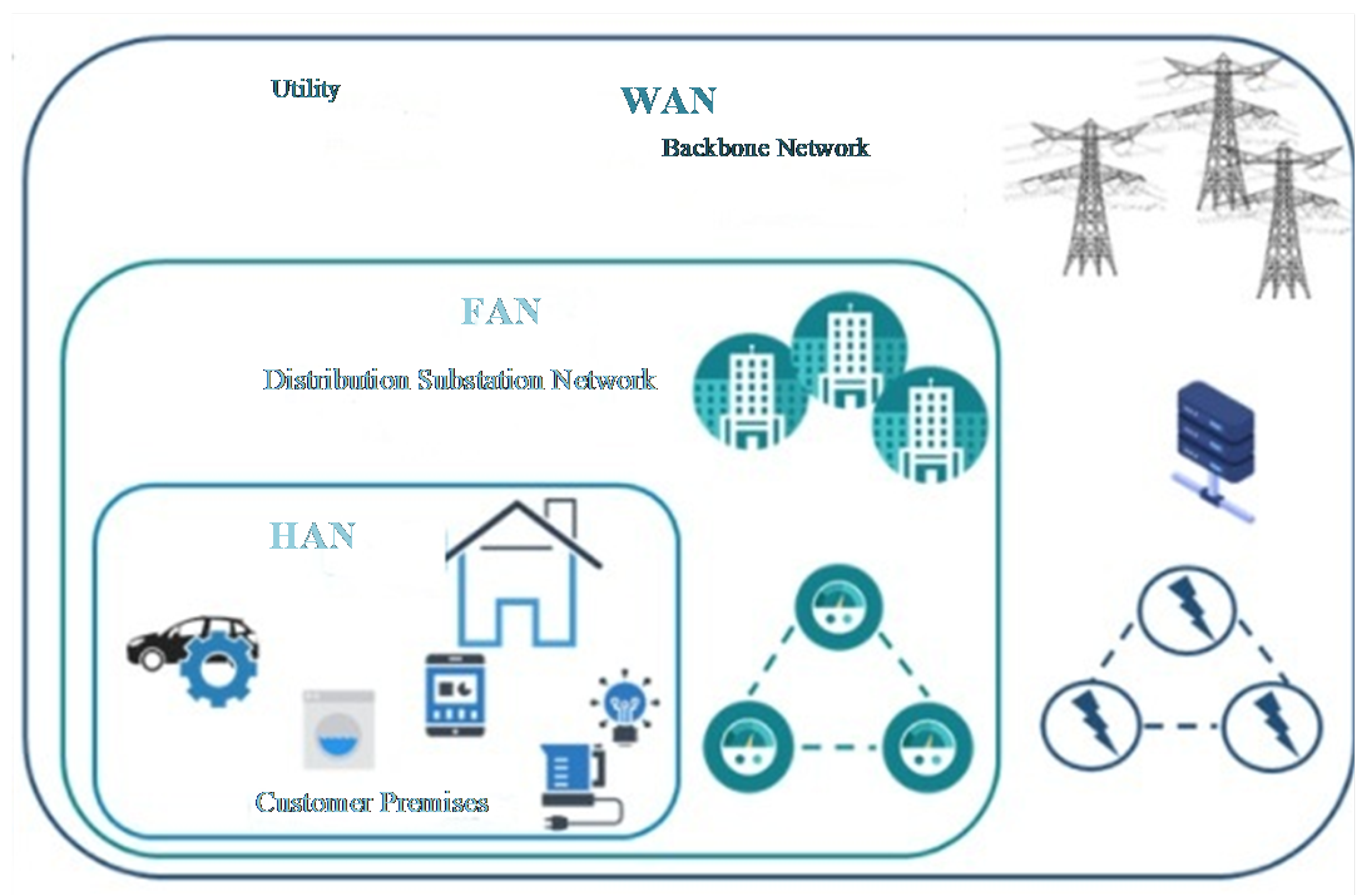
1.1. Smart Grid
1.2. Problem Statement and Motivation
2. Background and Related Work
2.1. Forecasting Electricity Load
2.2. Forecasting Electricity Price
3. System Models
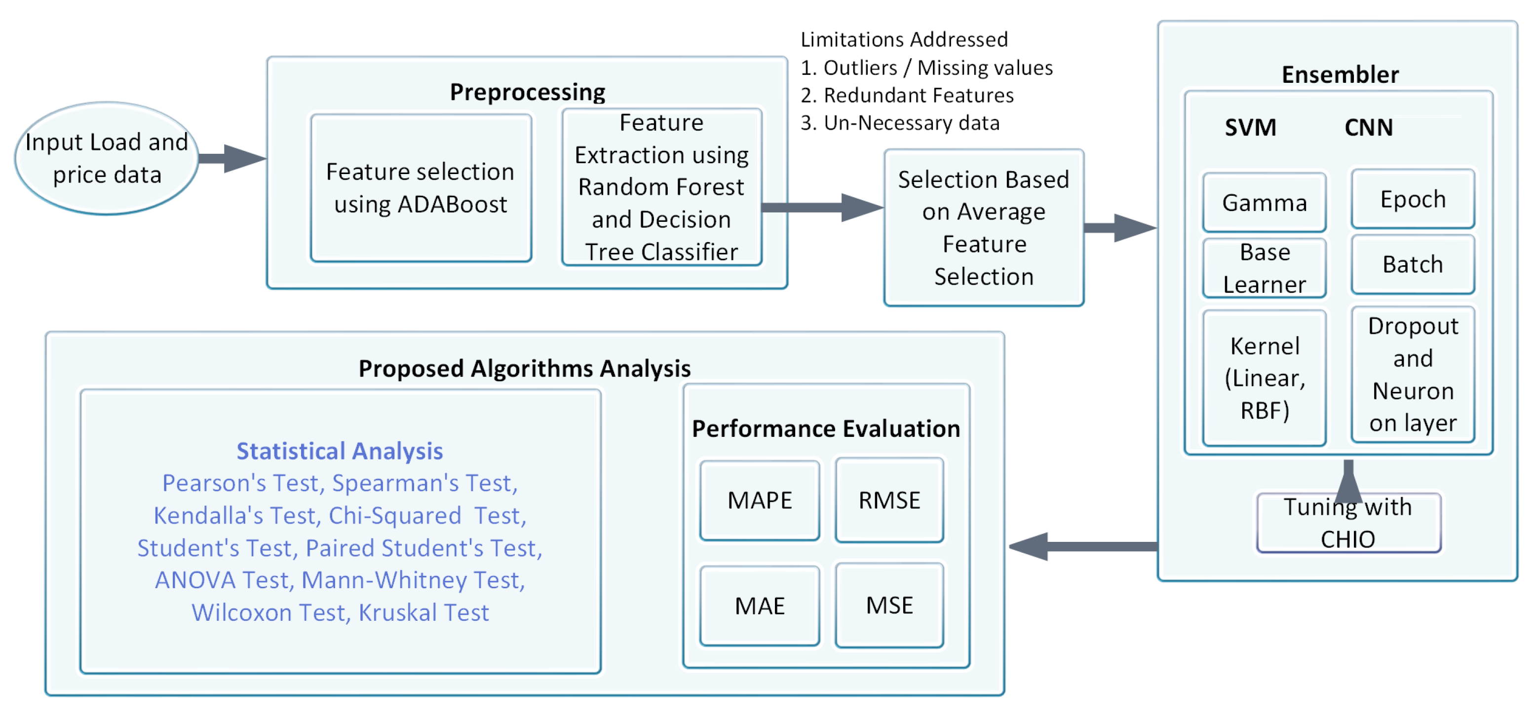
3.1. Model for Predicting Electricity Load and Price
- Data input (i.e., dataset).
- Feature extraction using RFE.
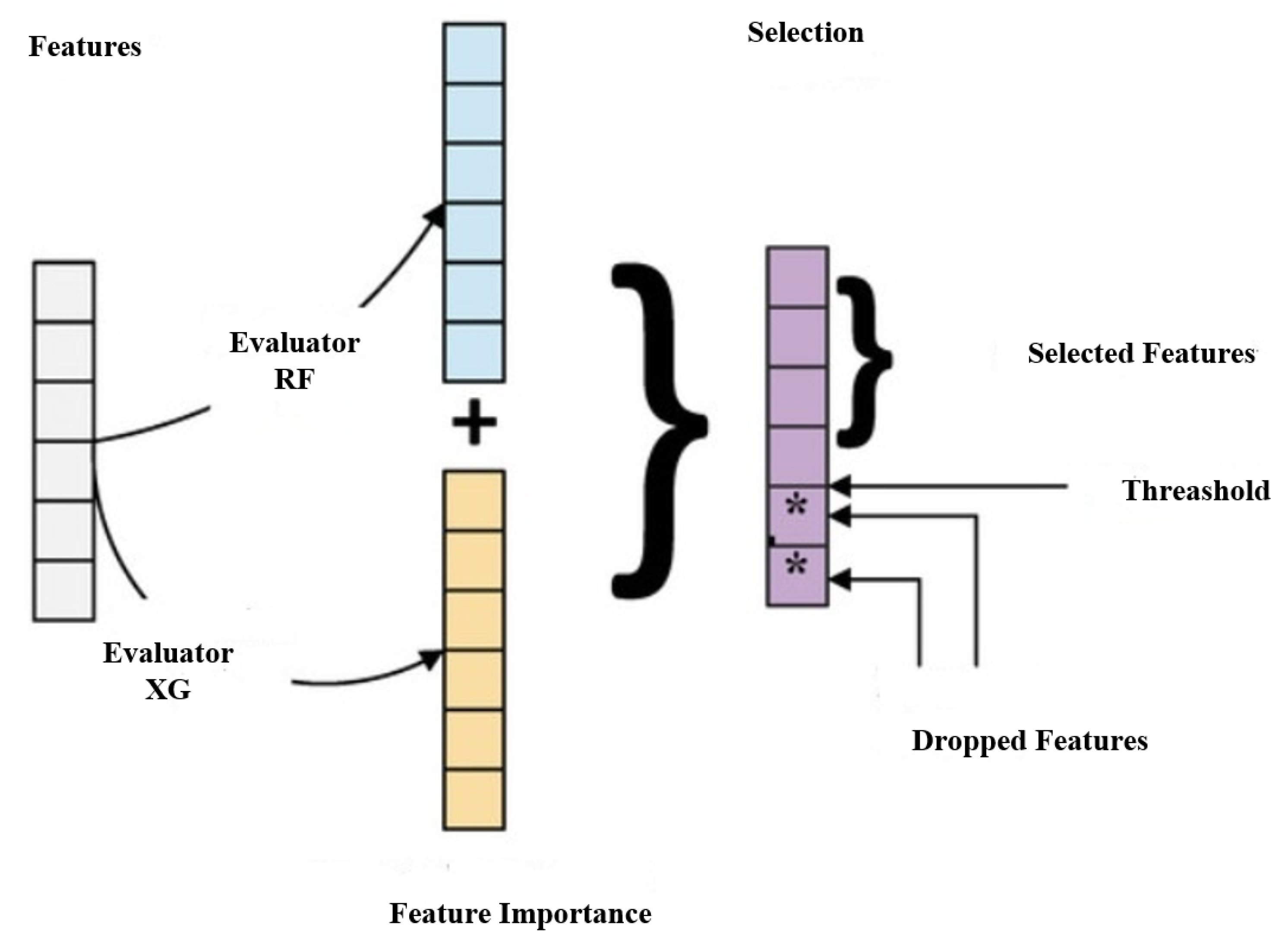
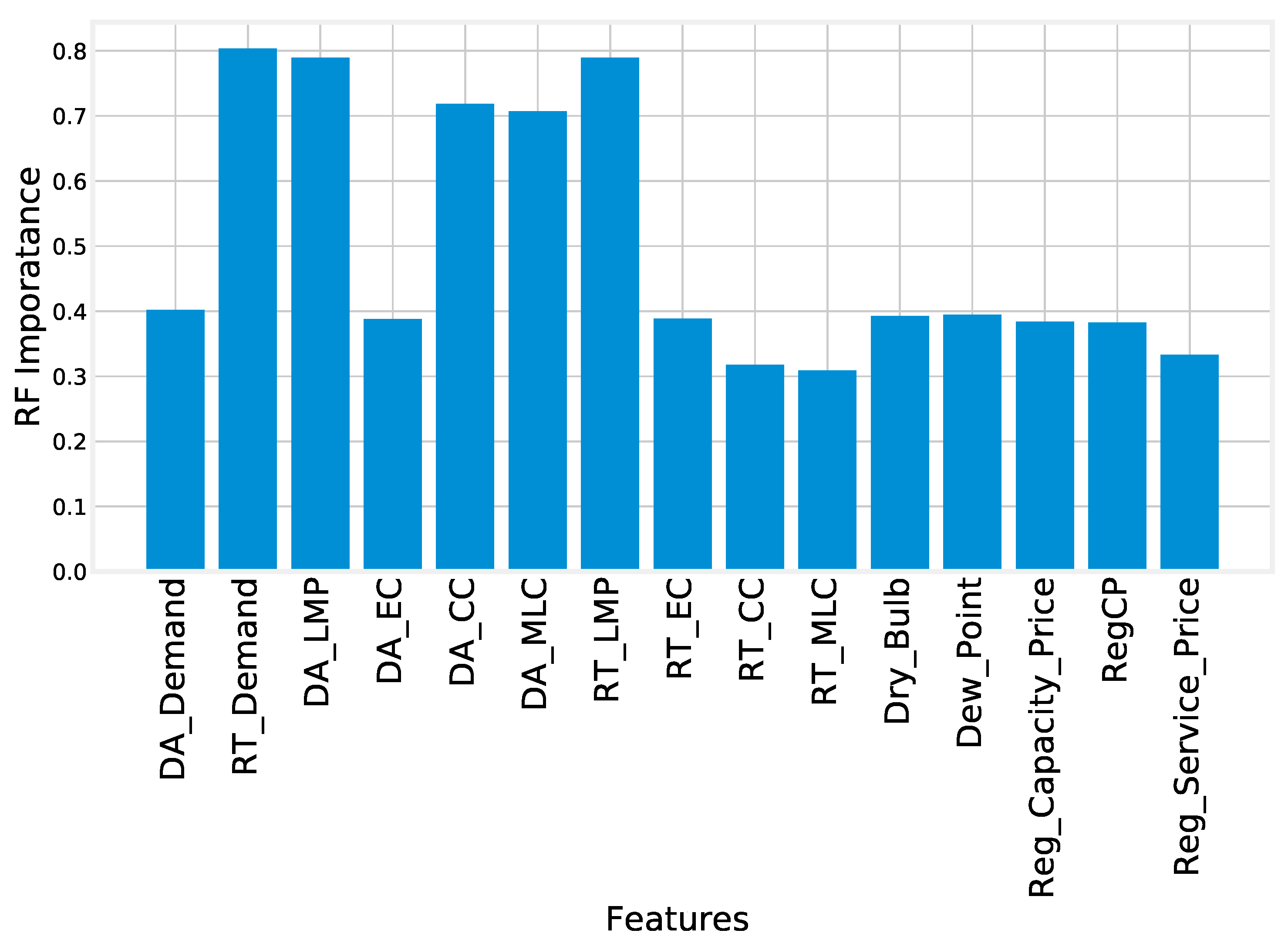
- Feature selection using RF and XG-Boost.
- Splitting of data into training and testing.
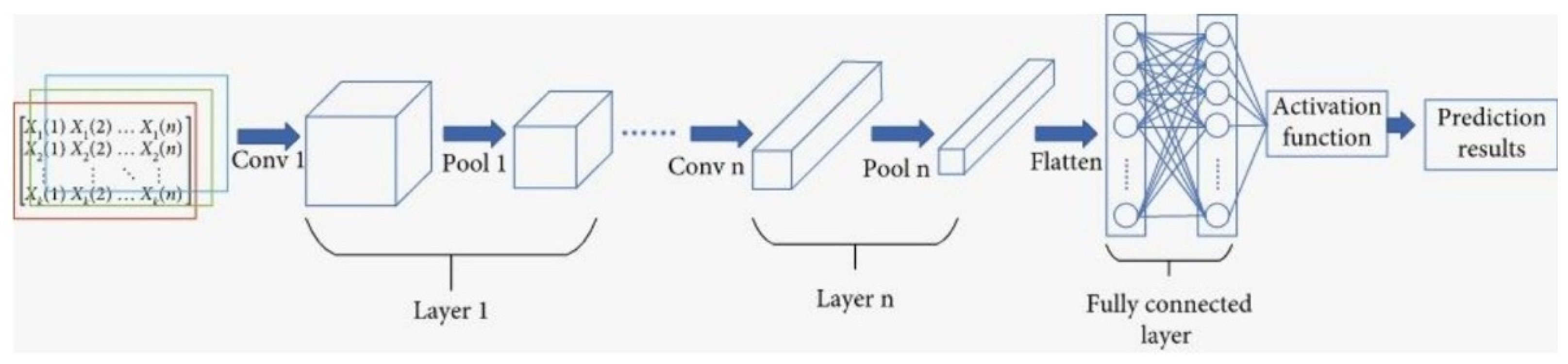
- Load the CNN layers and parameters.
- Tuning the CNN parameters using CHIO and then model compiling.
- Predicted price and load.
- Performance evaluation.
- Statistical analysis.
3.2. Data Collection
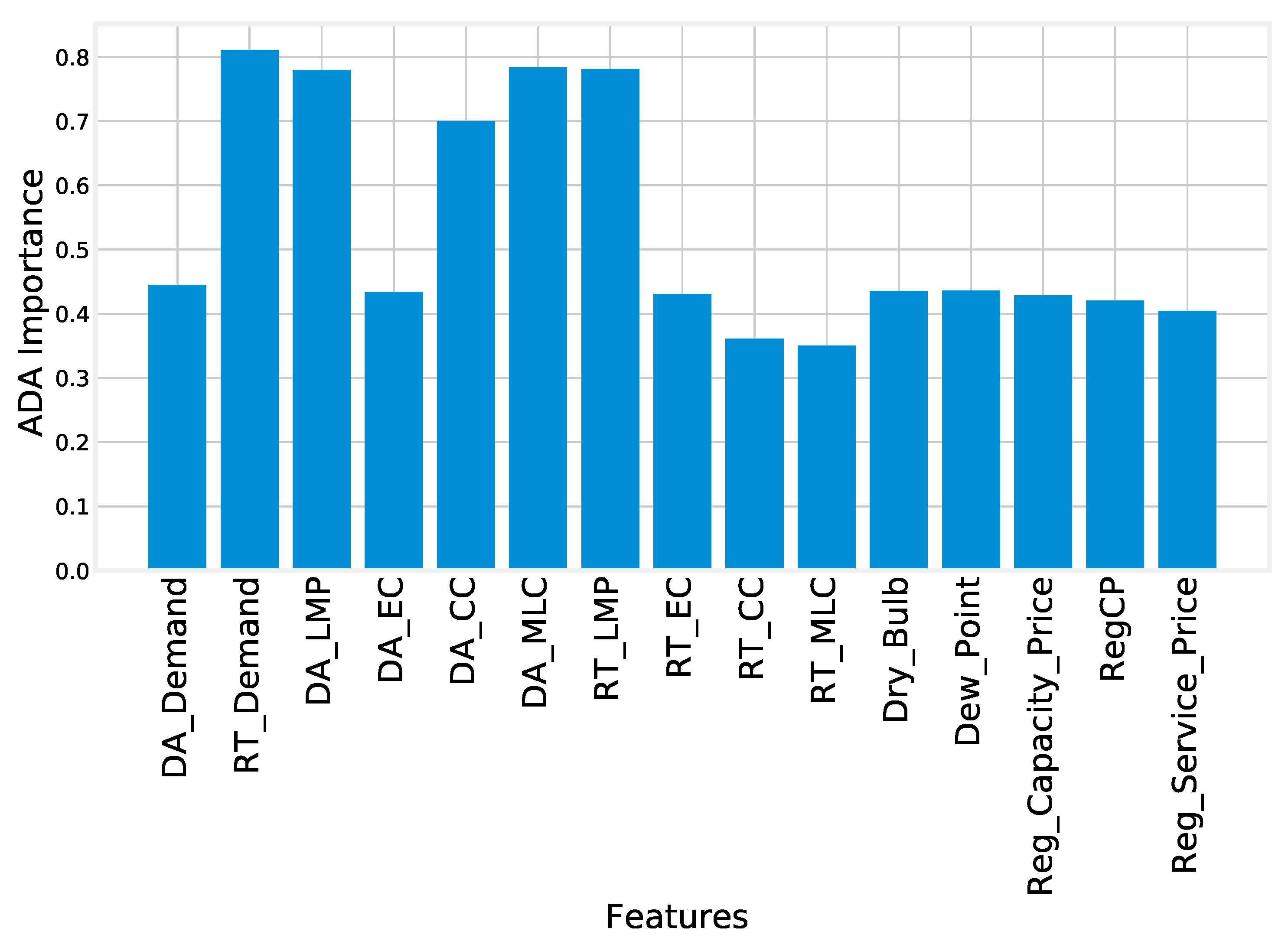
3.3. Feature Extraction Using (RFE)
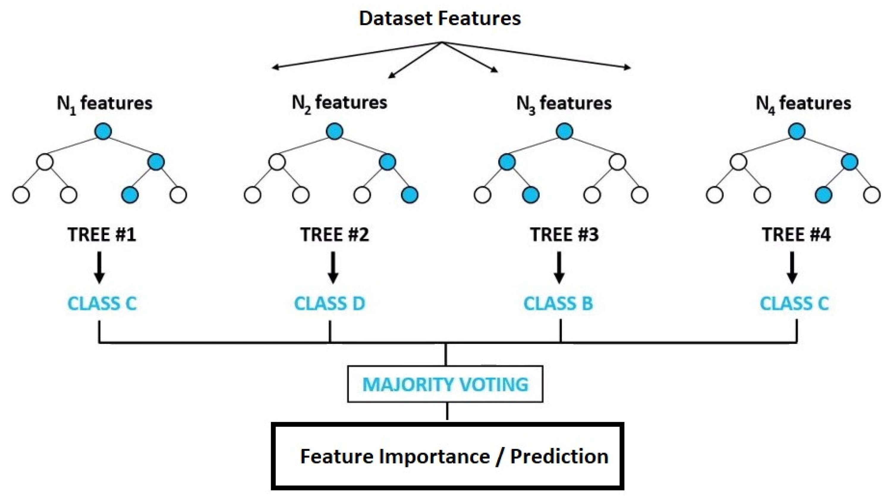
3.4. Feature Selection
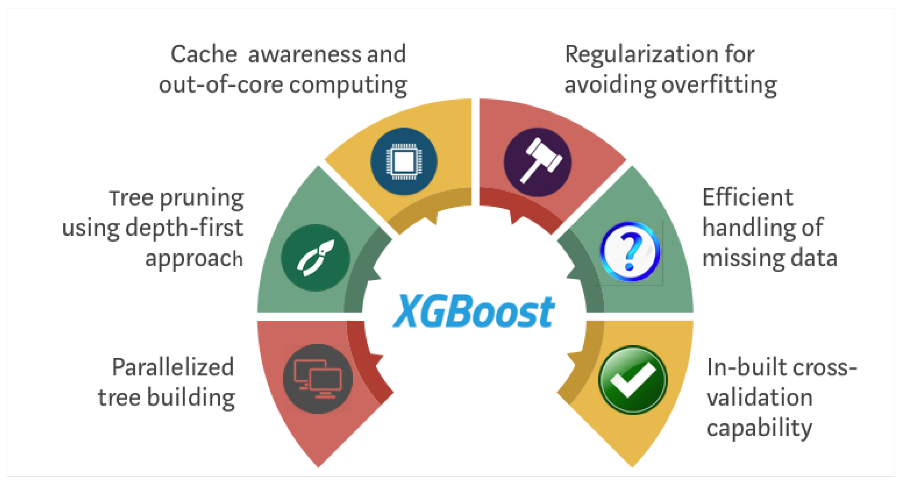
XG-Boost
3.5. Convolutional Neural Network
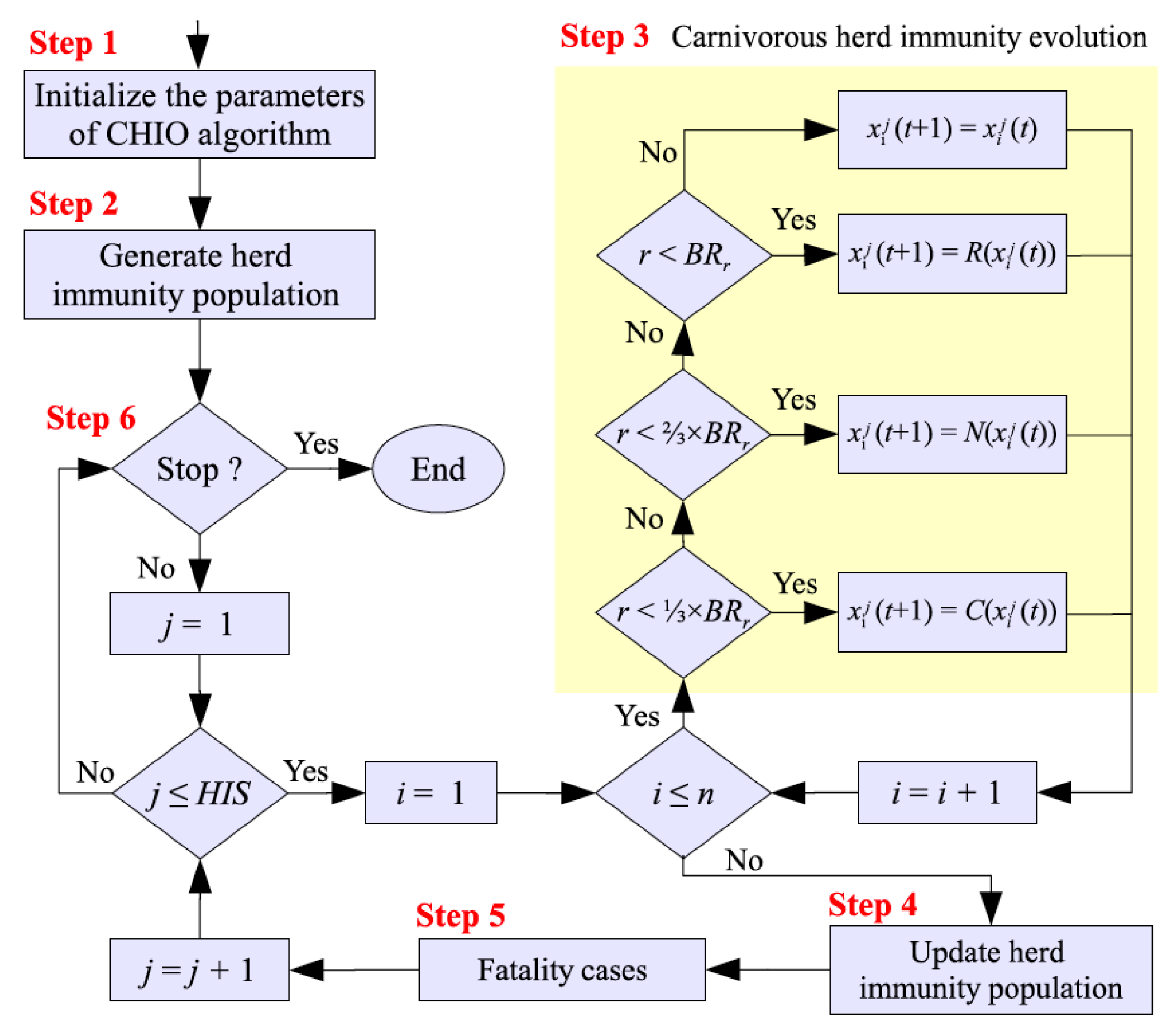
3.6. Coronavirus Herd Immunity Optimization
| Algorithm 1: Proposed Work Algorithm |
| Result: Electricity price and load forecasting X: data features; Y: data with a purpose; /* Separate the data into two categories: preparation and testing. */ ; split (x, y) = x train, x test, y train, y test; RFE (5, x train, y train); Selected_ function; /* Selection of hybrid features */ ; Incorporateimp = RFimp + XGimp; /* Using RF and XG-boost, measure value */ ; RF imp = RF calculates importance; /* RFE is a technique for extracting features. */ ; 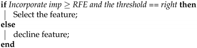 CNN-CHIO predicting the future with fine-tuned; Performance evaluation test, compare predictions; |
3.7. Performance Evaluation
4. Simulation Results and Discussions
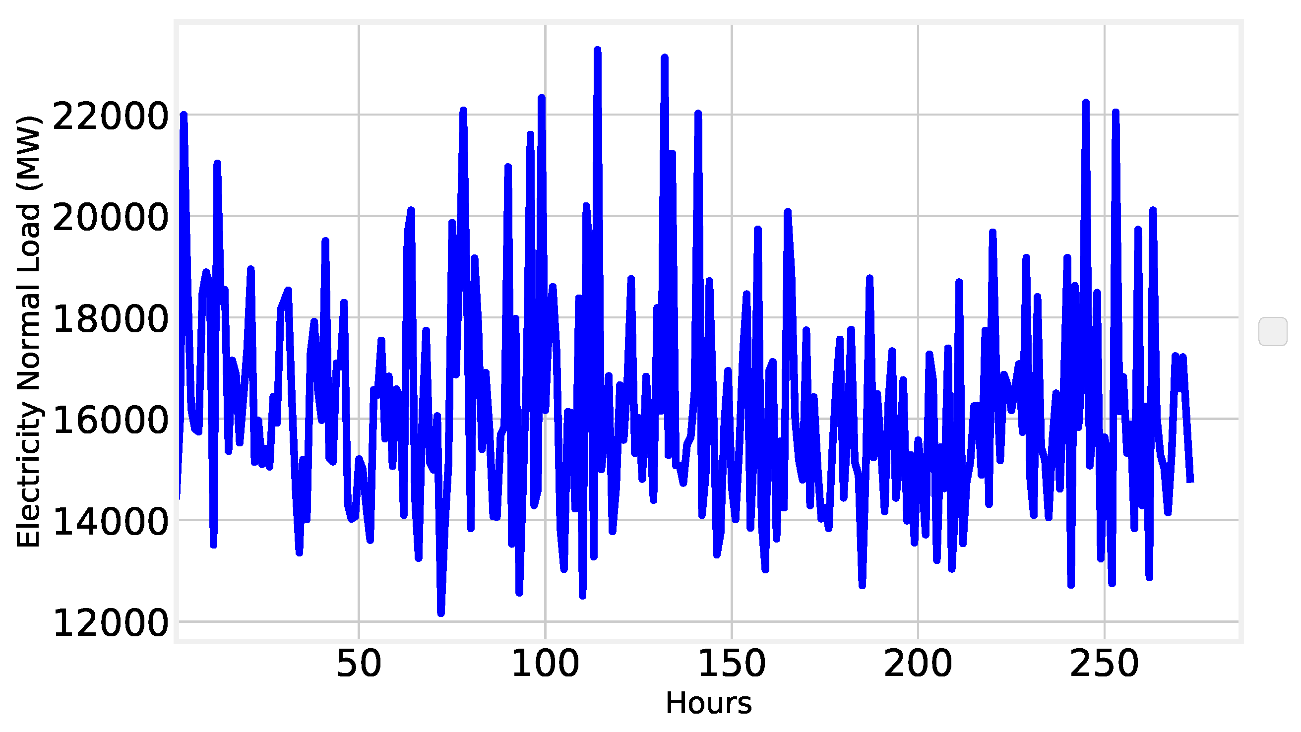
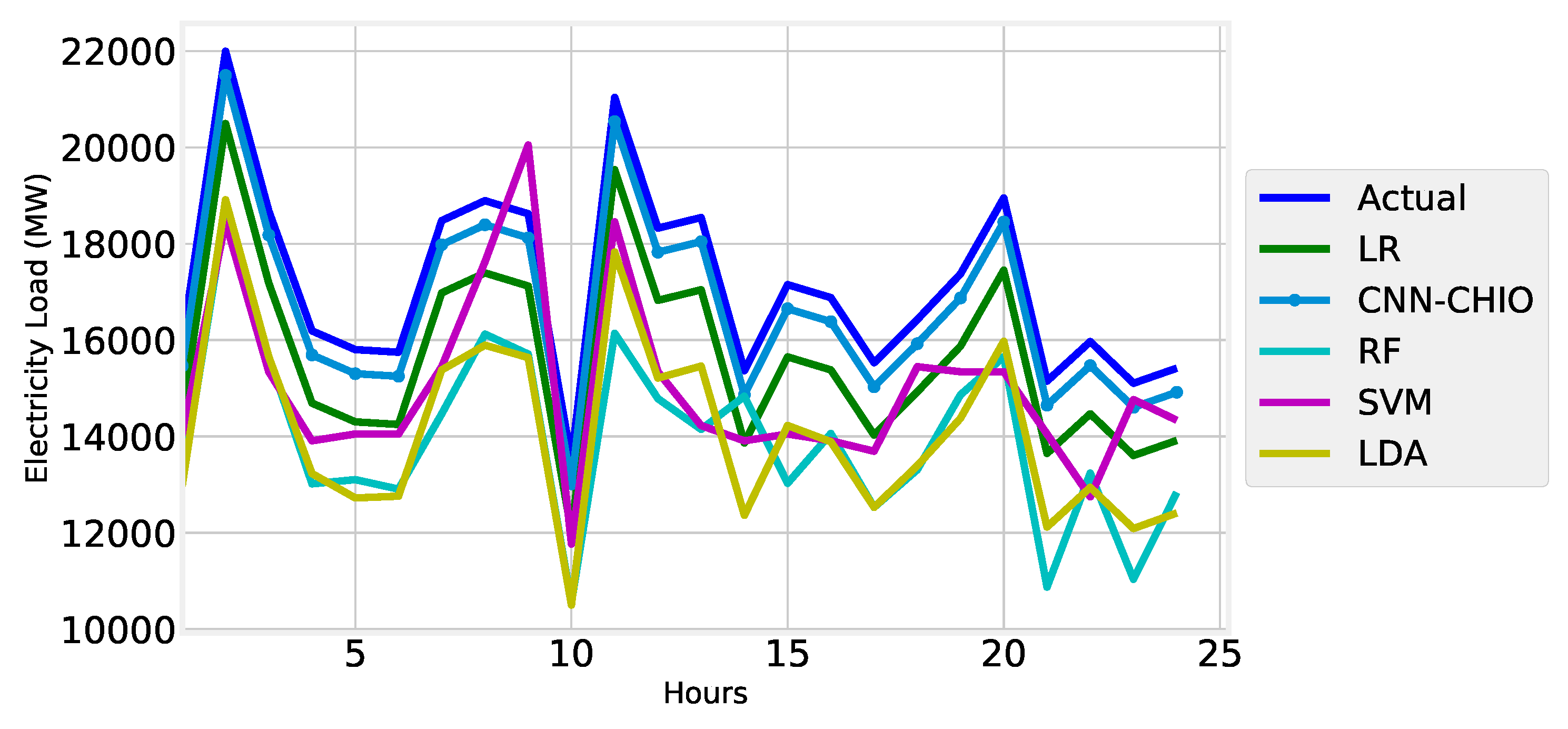
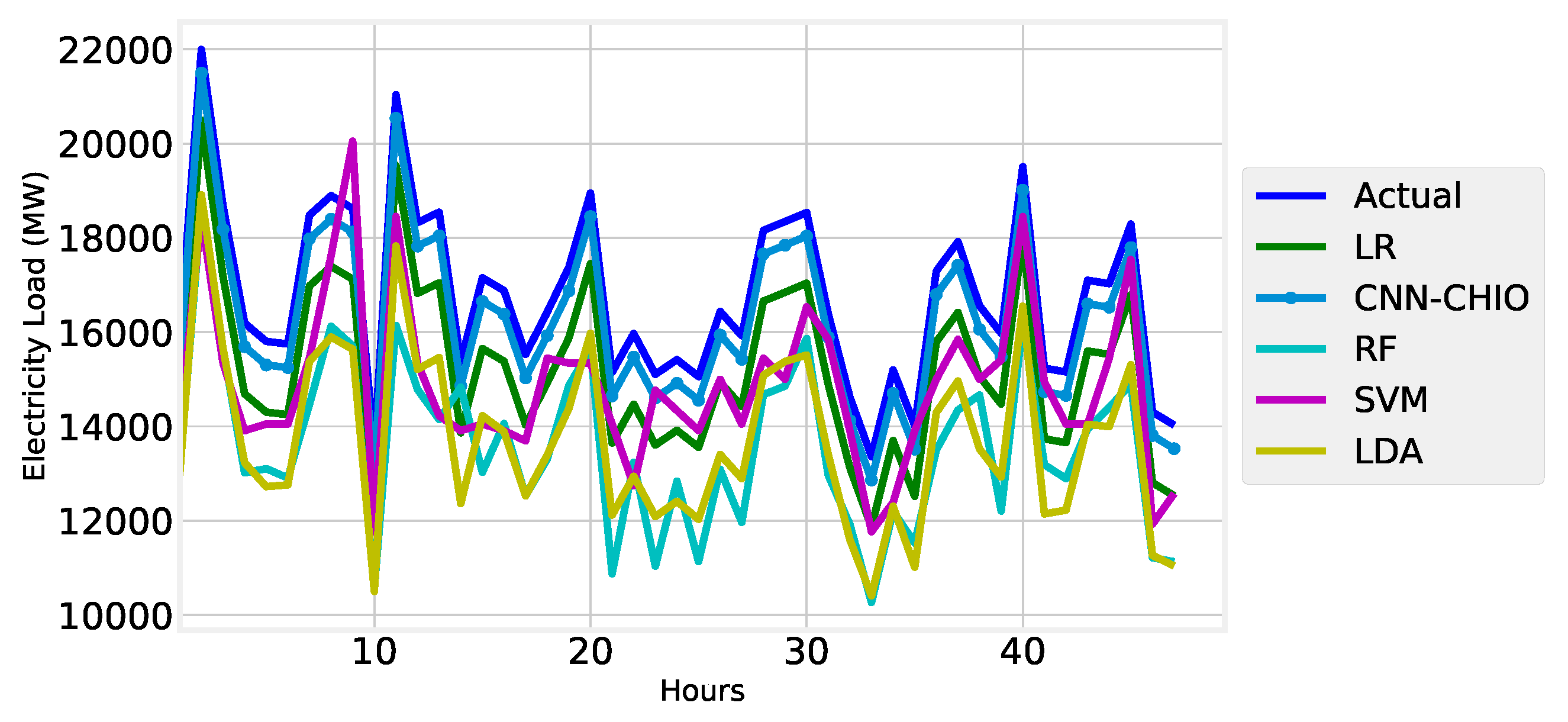
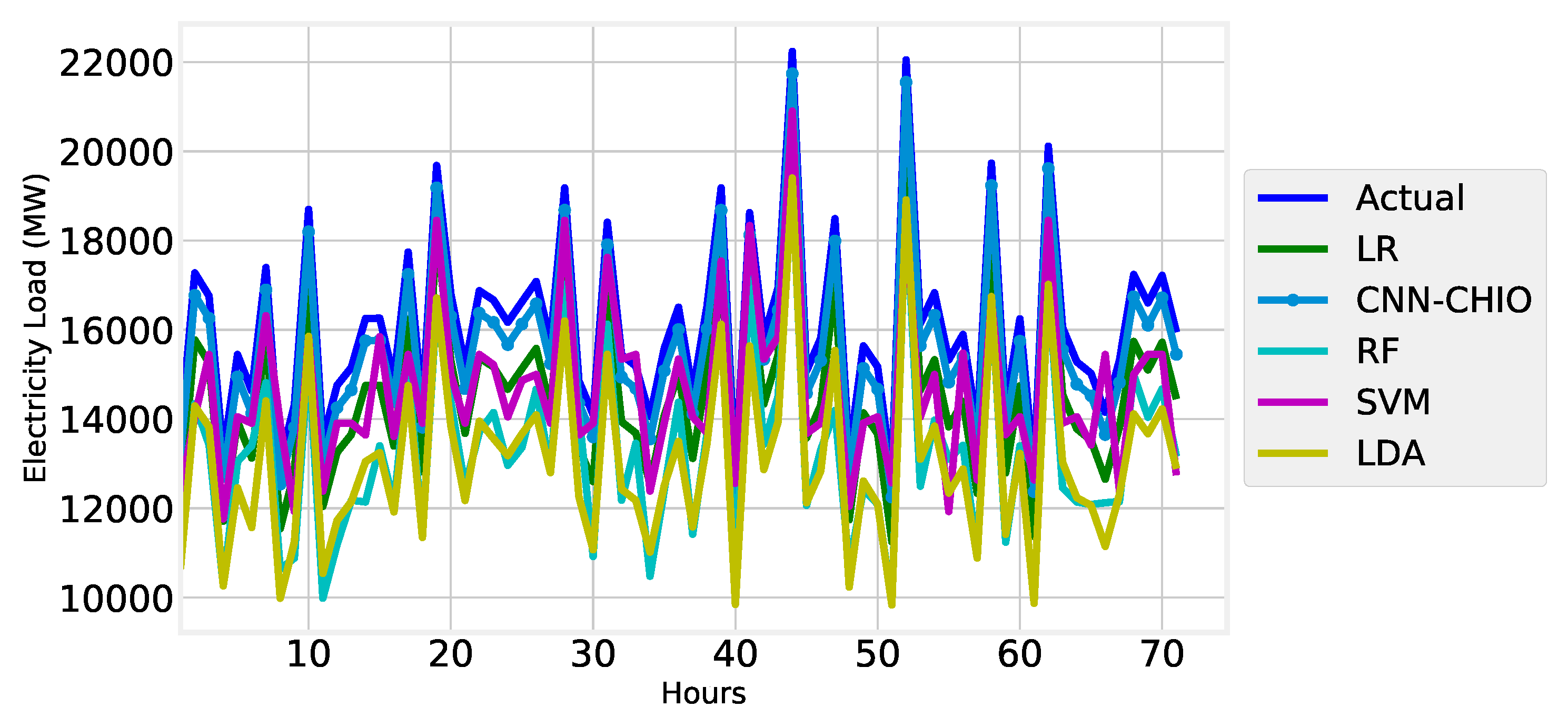
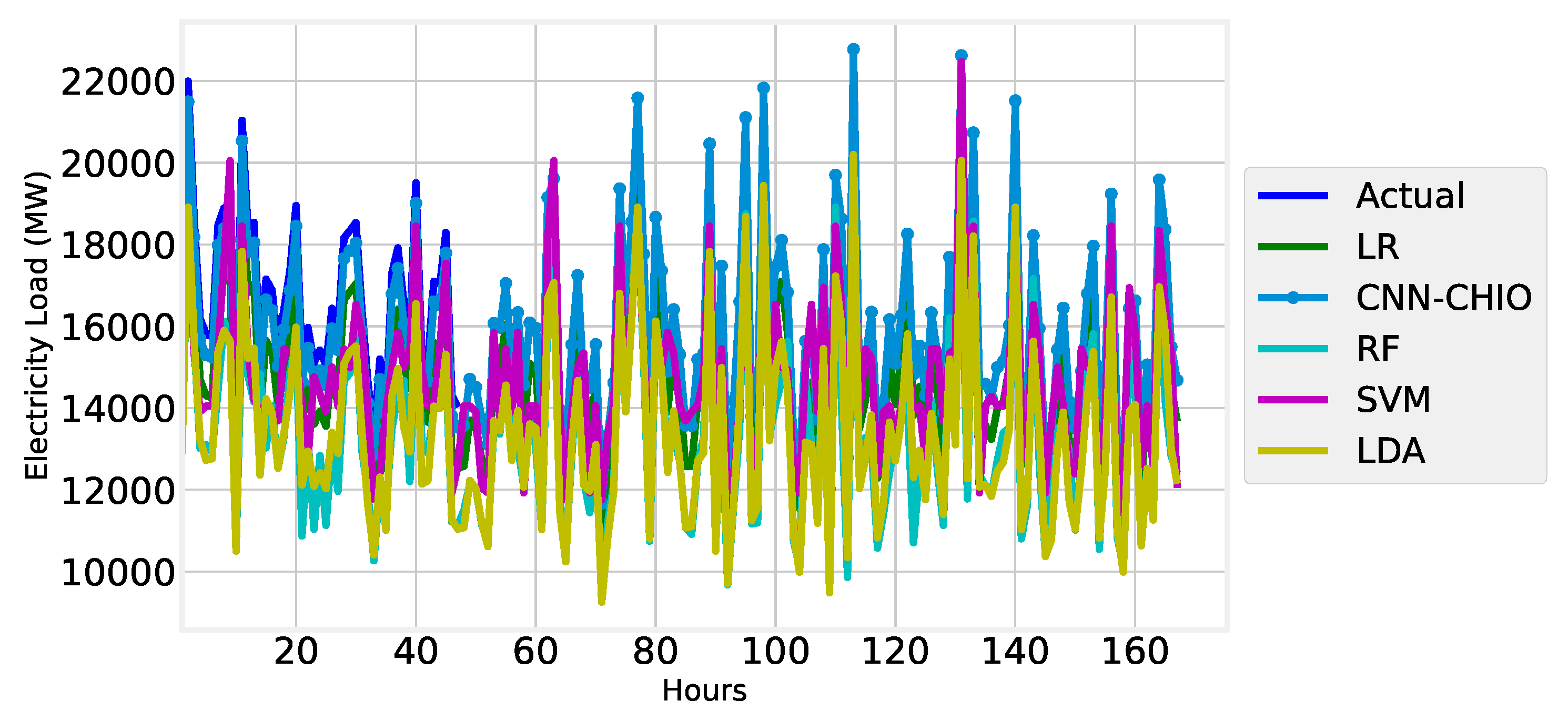
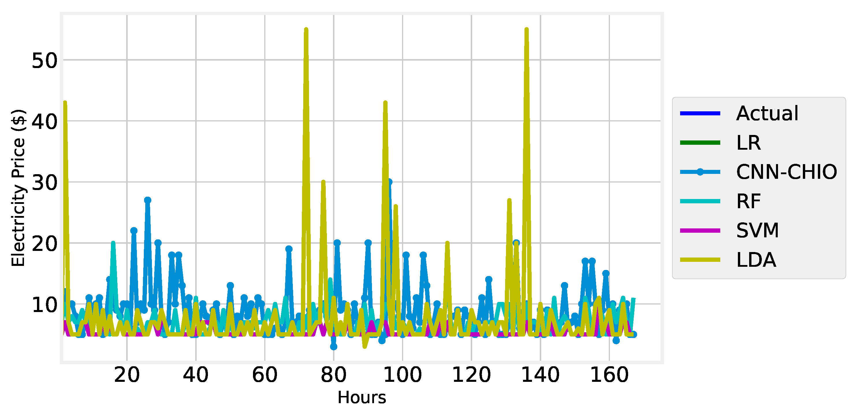
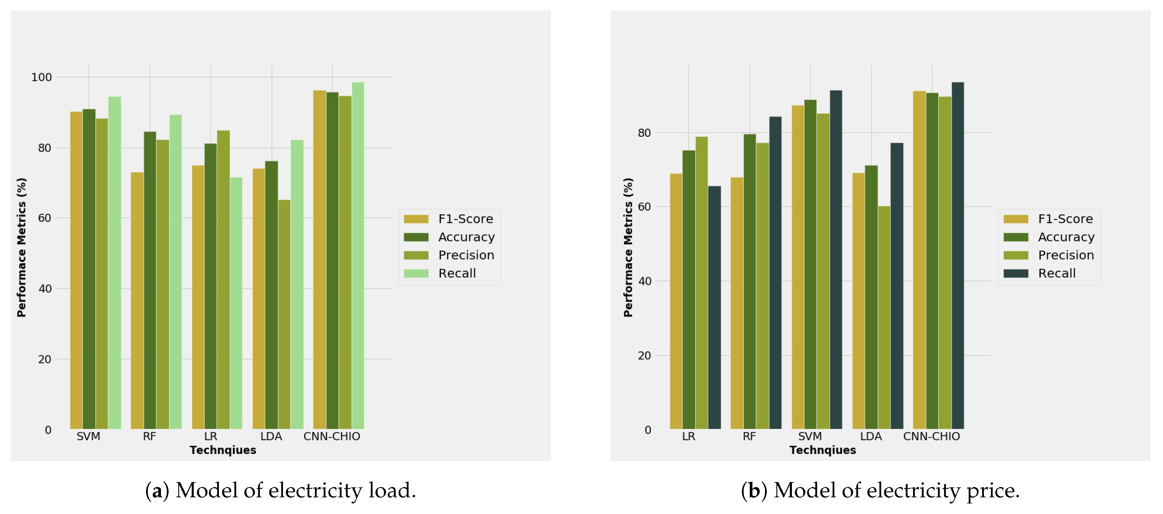
4.1. Electricity Load Forecasting
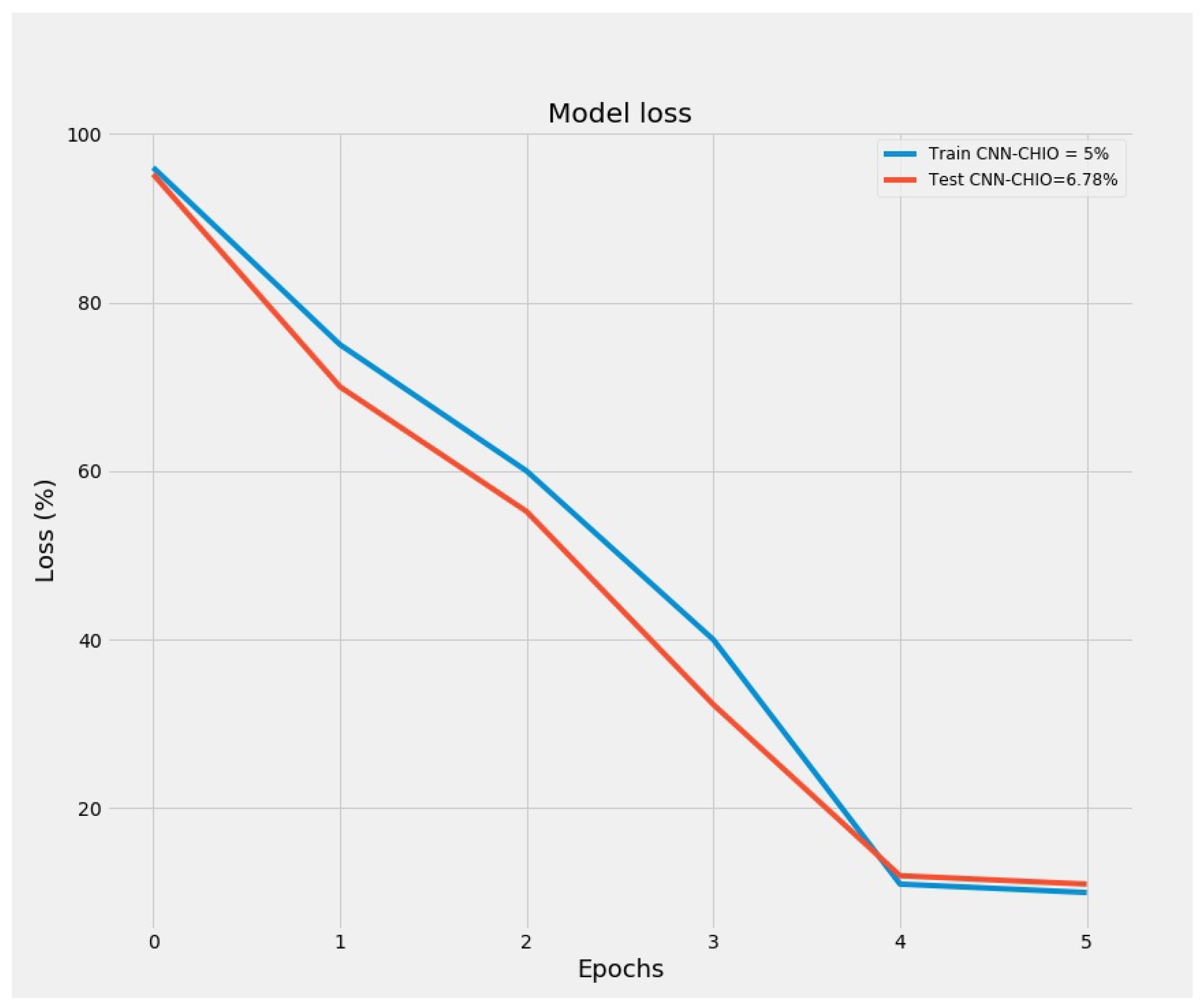
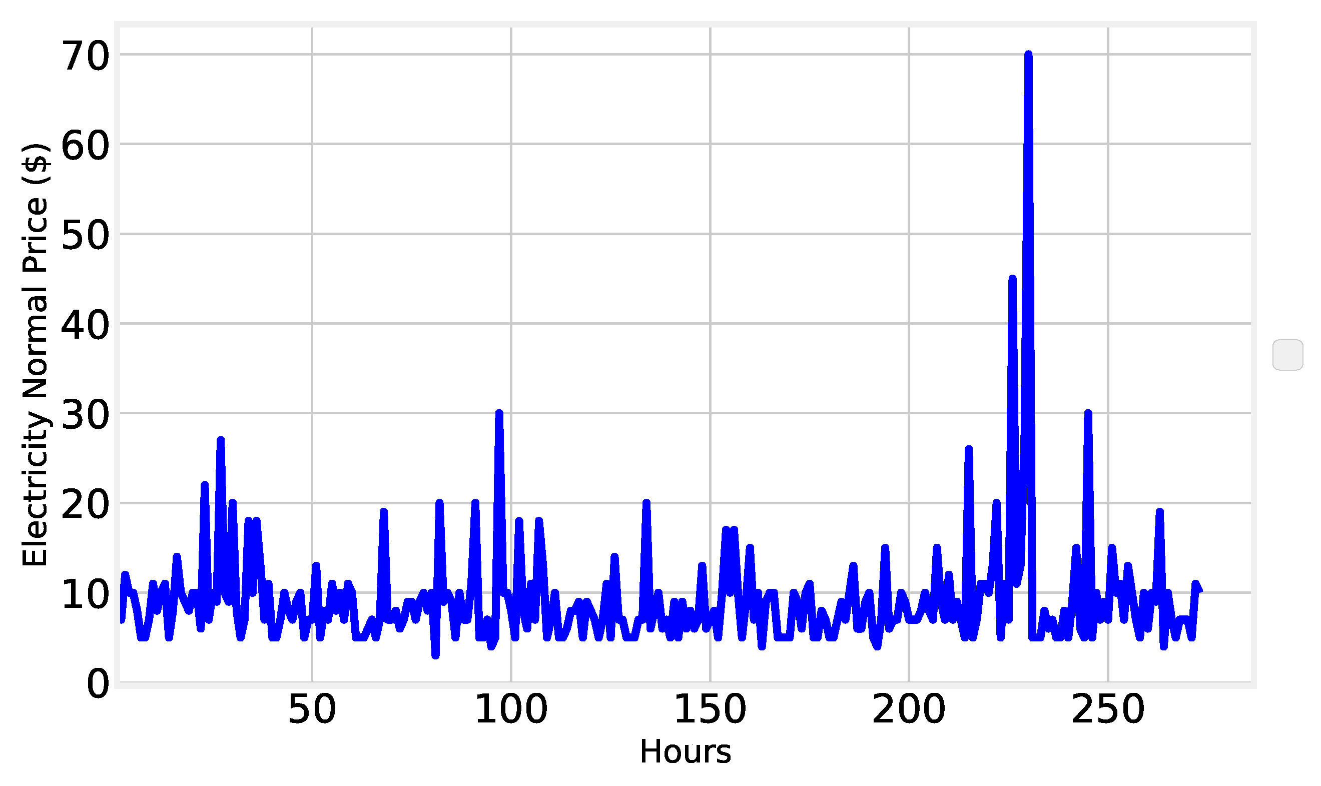
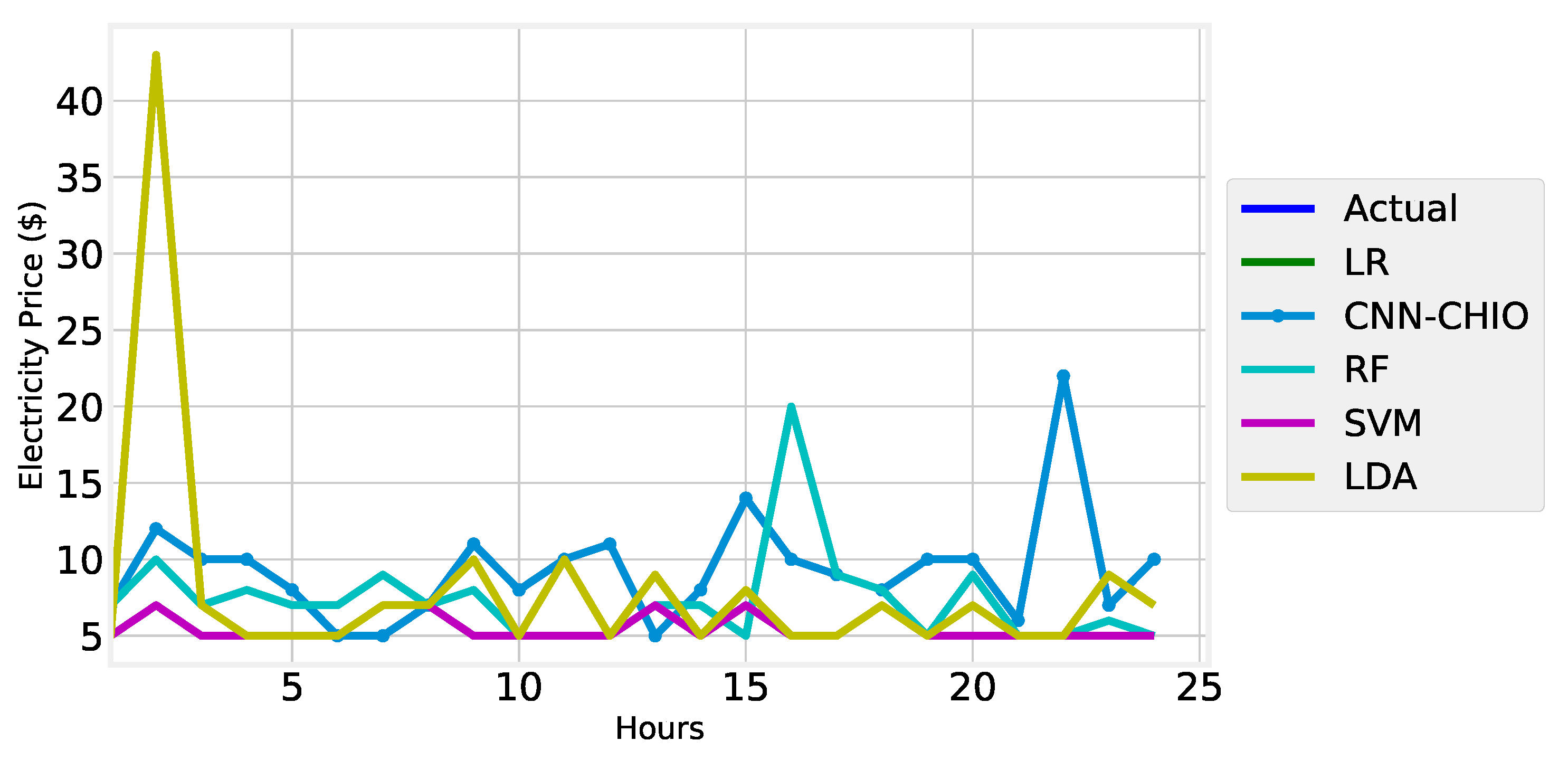
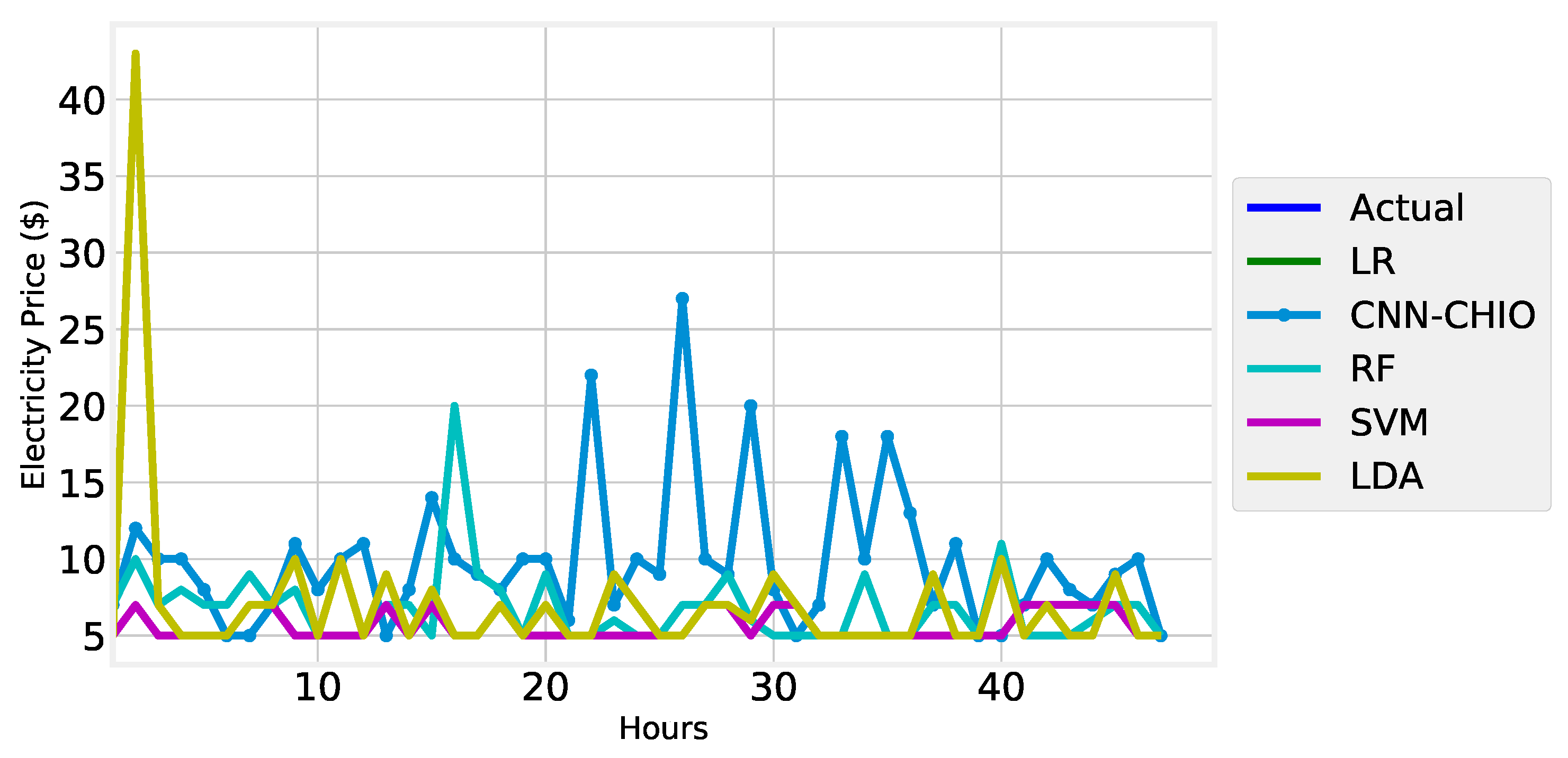
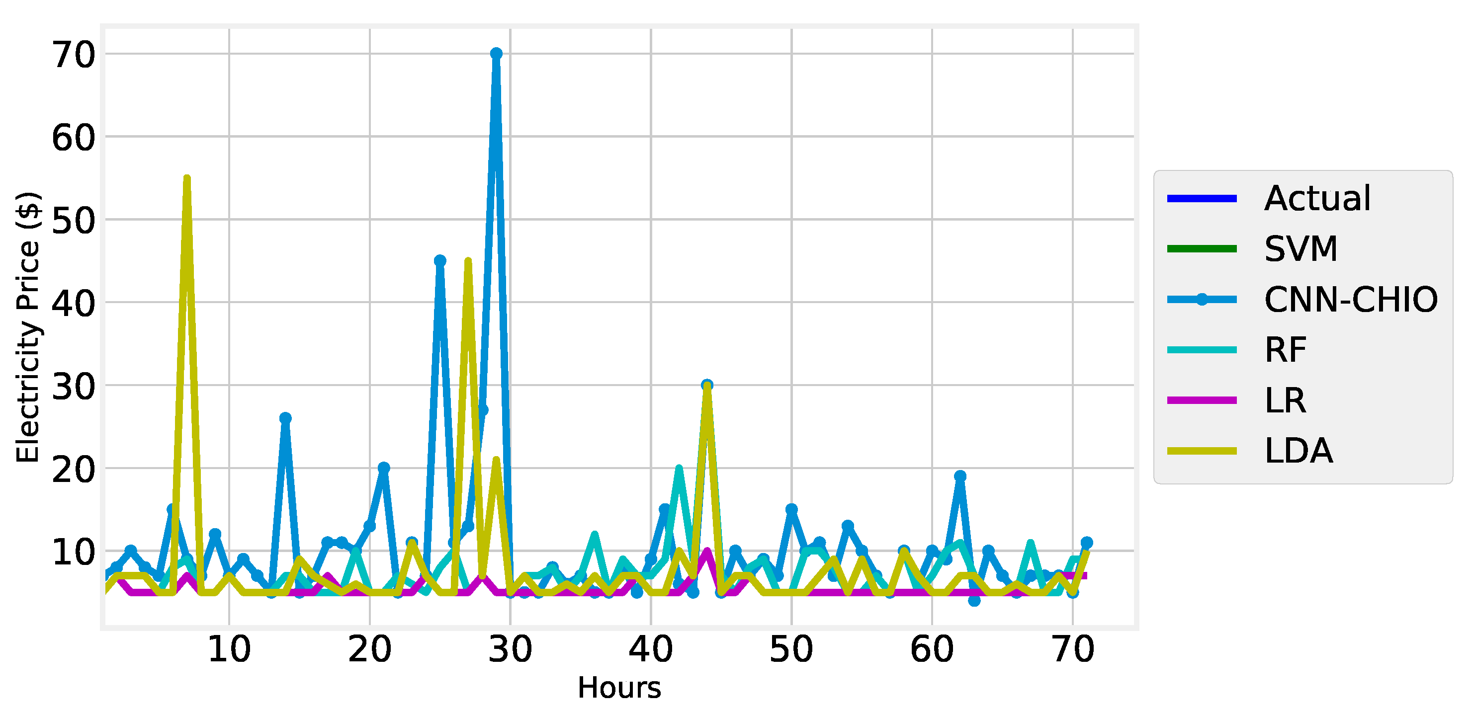
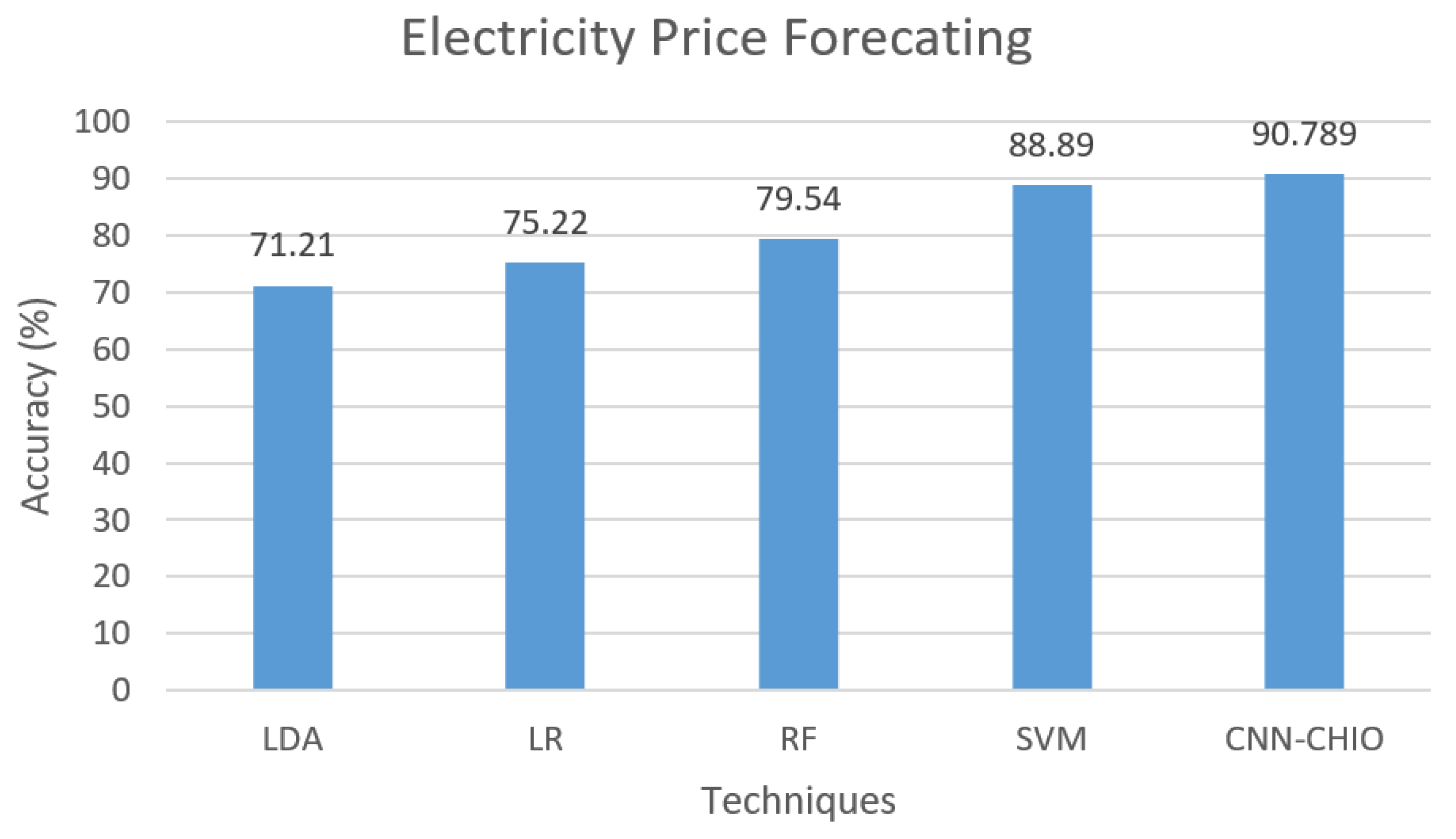
4.2. Electricity Price Forecasting
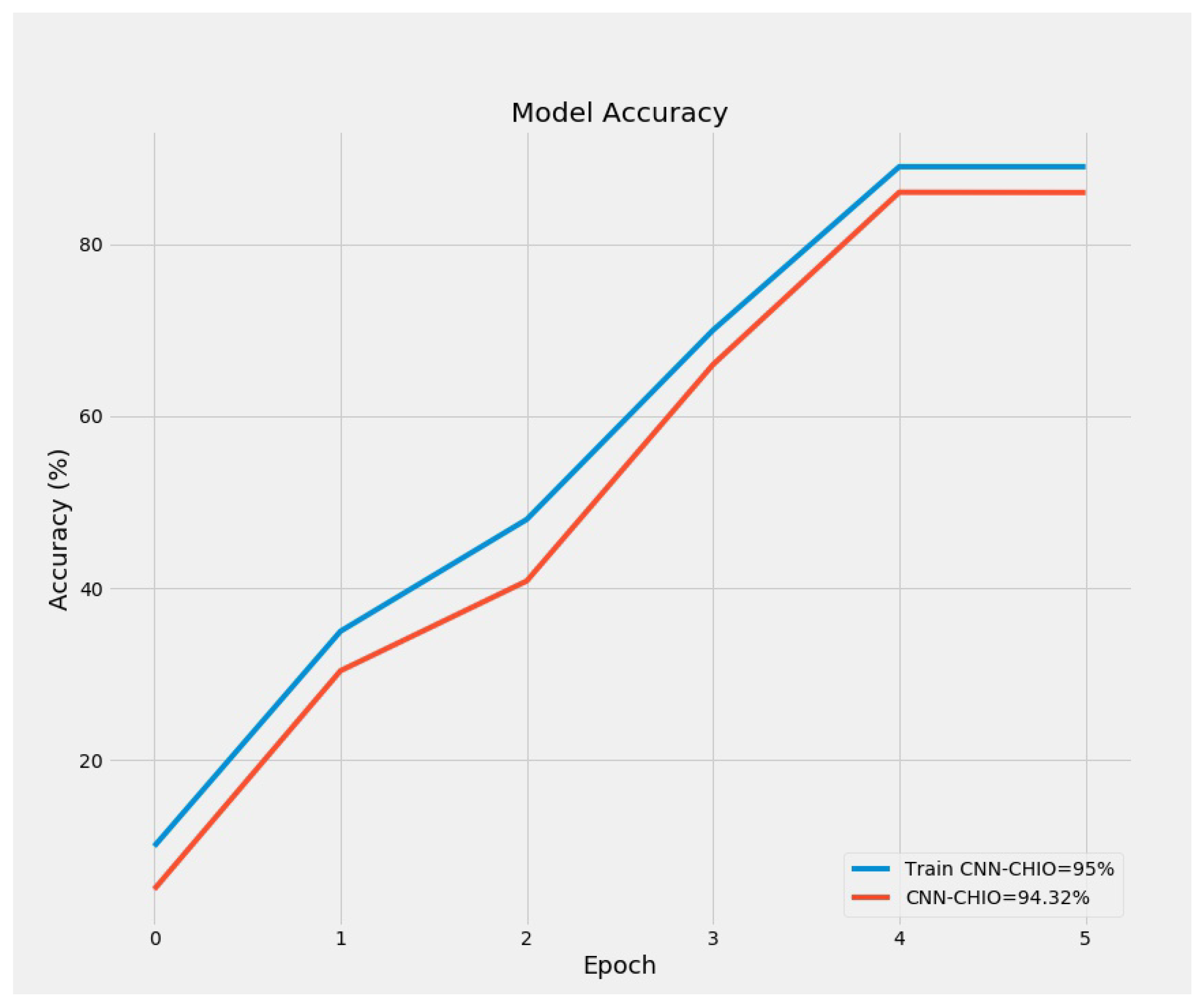
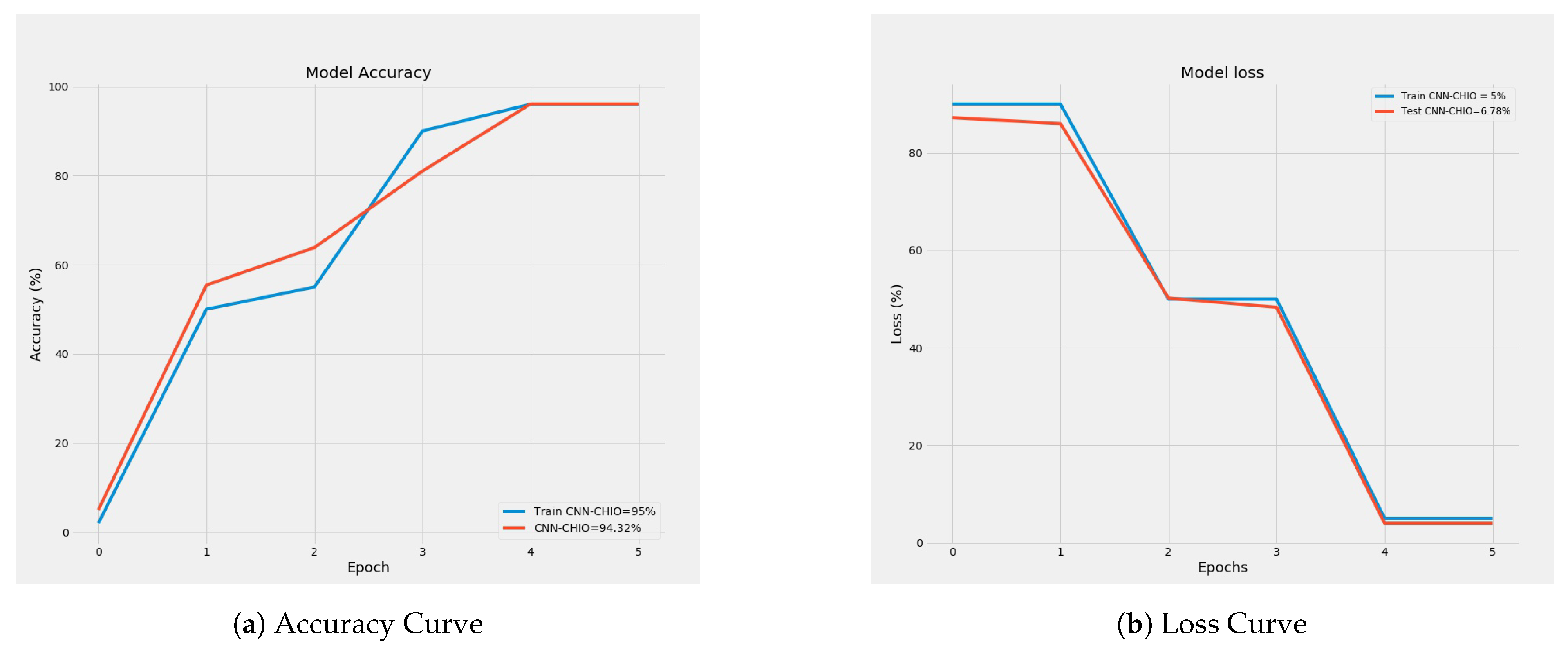
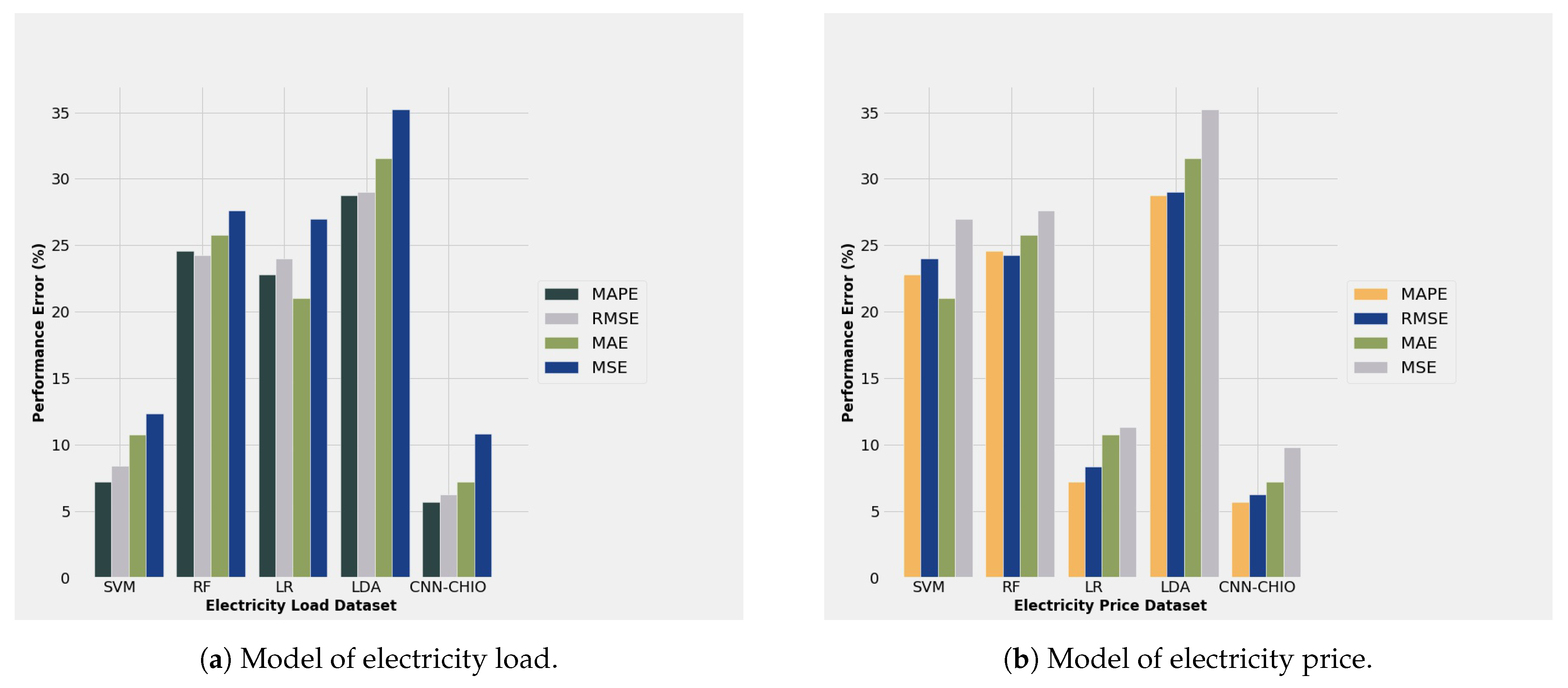
4.3. Performance Evaluation of Electricity Price and Load Forecasting
5. Conclusions
Author Contributions
Funding
Institutional Review Board Statement
Informed Consent Statement
Data Availability Statement
Acknowledgments
Conflicts of Interest
References
- Aslam, S.; Herodotou, H.; Mohsin, S.M.; Javaid, N.; Ashraf, N.; Aslam, S. A survey on deep learning methods for power load and renewable energy forecasting in smart microgrids. Renew. Sustain. Energy Rev. 2021, 144, 110992. [Google Scholar] [CrossRef]
- Liu, Y.; Yuen, C.; Huang, S.; Hassan, N.; Wang, X.; Xie, S. Peak-to-average ratio constrained demand-side management with consumer’s preference in residential smart grid. IEEE J. Sel. Top. Signal Process. 2014, 8, 1084–1097. [Google Scholar] [CrossRef]
- Aurangzeb, K.; Aslam, S.; Mohsin, S.M.; Alhussein, M. A fair pricing mechanism in smart grids for low energy consumption users. IEEE Access 2021, 9, 22035–22044. [Google Scholar] [CrossRef]
- Hor, C.L.; Watson, S.; Majithia, S. Analyzing the impact of weather variables on monthly electricity demand. IEEE Trans. Power Syst. 2005, 20, 2078–2085. [Google Scholar] [CrossRef]
- Siano, P. Demand response and smart grids—A survey. Renew. Sustain. Energy Rev. 2014, 30, 461–478. [Google Scholar] [CrossRef]
- Aslam, S.; Iqbal, Z.; Javaid, N.; Khan, Z.A.; Aurangzeb, K.; Haider, S.I. Towards efficient energy management of smart buildings exploiting heuristic optimization with real time and critical peak pricing schemes. Energies 2017, 10, 2065. [Google Scholar] [CrossRef] [Green Version]
- Liu, Y.; Wang, W.; Ghadimi, N. Electricity load forecasting by an improved forecast engine for building level consumers. Energy 2017, 139, 18–30. [Google Scholar] [CrossRef]
- Jin, X.B.; Zheng, W.Z.; Kong, J.L.; Wang, X.Y.; Bai, Y.T.; Su, T.L.; Lin, S. Deep-Learning Forecasting Method for Electric Power Load via Attention-Based Encoder-Decoder with Bayesian Optimization. Energies 2021, 14, 1596. [Google Scholar] [CrossRef]
- Li, Y.; Kubicki, S.; Guerriero, A.; Rezgui, Y. Review of building energy performance certification schemes towards future improvement. Renew. Sustain. Energy Rev. 2019, 113, 109244. [Google Scholar] [CrossRef]
- Carmichael, R.; Gross, R.; Hanna, R.; Rhodes, A.; Green, T. The Demand Response Technology Cluster: Accelerating UK residential consumer engagement with time-of-use tariffs, electric vehicles and smart meters via digital comparison tools. Renew. Sustain. Energy Rev. 2021, 139, 110701. [Google Scholar] [CrossRef]
- Ghosal, A.; Conti, M. Key management systems for smart grid advanced metering infrastructure: A survey. IEEE Commun. Surv. Tutor. 2019, 21, 2831–2848. [Google Scholar] [CrossRef] [Green Version]
- Dileep, G. A survey on smart grid technologies and applications. Renew. Energy 2020, 146, 2589–2625. [Google Scholar] [CrossRef]
- Kuo, P.H.; Huang, C.J. An electricity price forecasting model by hybrid structured deep neural networks. Sustainability 2018, 10, 1280. [Google Scholar] [CrossRef] [Green Version]
- Ugurlu, U.; Oksuz, I.; Tas, O. Electricity price forecasting using recurrent neural networks. Energies 2018, 11, 1255. [Google Scholar] [CrossRef] [Green Version]
- Eapen, R.; Simon, S. Performance analysis of combined similar day and day ahead short term electrical load forecasting using sequential hybrid neural networks. IETE J. Res. 2019, 65, 216–226. [Google Scholar] [CrossRef]
- Zhang, X.; Wang, J.; Zhang, K. Short-term electric load forecasting based on singular spectrum analysis and support vector machine optimized by Cuckoo search algorithm. Electr. Power Syst. Res. 2017, 146, 270–285. [Google Scholar] [CrossRef]
- Patil, M.; Deshmukh, S.; Agrawal, R. Electric power price forecasting using data mining techniques. In Proceedings of the 2017 International Conference on Data Management, Analytics and Innovation (ICDMAI), Pune, India, 24–26 February 2017; pp. 217–223. [Google Scholar]
- Bouktif, S.; Fiaz, A.; Ouni, A.; Serhani, M. Optimal deep learning lstm model for electric load forecasting using feature selection and genetic algorithm: Comparison with machine learning approaches. Energies 2018, 11, 1636. [Google Scholar] [CrossRef] [Green Version]
- Keles, D.; Scelle, J.; Paraschiv, F.; Fichtner, W. Extended forecast methods for day-ahead electricity spot prices applying artificial neural networks. Appl. Energy 2016, 162, 218–230. [Google Scholar] [CrossRef]
- Ma, Z.; Zhong, H.; Xie, L.; Xia, Q.; Kang, C. Month ahead average daily electricity price profile forecasting based on a hybrid nonlinear regression and SVM model: An ERCOT case study. J. Mod. Power Syst. Clean Energy 2018, 6, 281–291. [Google Scholar] [CrossRef]
- Lago, J.; De Ridder, F.; De Schutter, B. Forecasting spot electricity prices: Deep learning approaches and empirical comparison of traditional algorithms. Appl. Energy 2018, 221, 386–405. [Google Scholar] [CrossRef]
- Ghadimi, N.; Akbarimajd, A.; Shayeghi, H.; Abedinia, O. Two stage forecast engine with feature selection technique and improved meta-heuristic algorithm for electricity load forecasting. Energy 2018, 161, 130–142. [Google Scholar] [CrossRef]
- Jindal, A.; Singh, M.; Kumar, N.; Response, C.A. Scheme for Peak Load Reduction in Smart Grid. IEEE Trans. Ind. Electron. 2018, 65, 8993–9004. [Google Scholar] [CrossRef]
- Chitsaz, H.; Zamani-Dehkordi, P.; Zareipour, H.; Parikh, P. Electricity price forecasting for operational scheduling of behind-the-meter storage systems. IEEE Trans. Smart Grid 2017, 9, 6612–6622. [Google Scholar] [CrossRef]
- Pérez-Chacón, R.; Luna-Romera, J.M.; Troncoso, A.; Martínez-Álvarez, F.; Riquelme, J.C. Big data analytics for discovering electricity consumption patterns in smart cities. Energies 2018, 11, 683. [Google Scholar] [CrossRef] [Green Version]
- Wang, Z.; Wang, Y.; Zeng, R.; Srinivasan, R.; Ahrentzen, S. Random Forest based hourly building energy prediction. Energy Build. 2018, 171, 11–25. [Google Scholar] [CrossRef]
- Lahouar, A.; Slama, J. Day-ahead load forecast using random forest and expert input selection. Energy Convers. Manag. 2015, 103, 1040–1051. [Google Scholar] [CrossRef]
- Wang, K.; Xu, C.; Zhang, Y.; Guo, S.; Zomaya, A. Robust big data analytics for electricity price forecasting in the smart grid. IEEE Trans. Big Data 2017, 5, 34–45. [Google Scholar] [CrossRef]
- Wang, L.; Zhang, Z.; Chen, J. Short-term electricity price forecasting with stacked denoising autoencoders. IEEE Trans. Power Syst. 2016, 32, 2673–2681. [Google Scholar] [CrossRef]
- Lago, J.; De Ridder, F.; Vrancx, P.; De Schutter, B. Forecasting day-ahead electricity prices in Europe: The importance of considering market integration. Appl. Energy 2018, 211, 890–903. [Google Scholar] [CrossRef]
- Raviv, E.; Bouwman, K.; Van Dijk, D. Forecasting day-ahead electricity prices: Utilizing hourly prices. Energy Econ. 2015, 50, 227–239. [Google Scholar] [CrossRef] [Green Version]
- Mujeeb, S.; Javaid, N.; Akbar, M.; Khalid, R.; Nazeer, O.; Khan, M. Big data analytics for price and load forecasting in smart grids. In Proceedings of the International Conference on Broadband and Wireless Computing, Communication and Applications, Taichung, Taiwan, 27–29 October 2018; pp. 77–87. [Google Scholar]
- Rafiei, M.; Niknam, T.; Khooban, M.H. Probabilistic forecasting of hourly electricity price by generalization of ELM for usage in improved wavelet neural network. IEEE Trans. Ind. Inform. 2016, 13, 71–79. [Google Scholar] [CrossRef]
- Abedinia, O.; Amjady, N.; Zareipour, H. A new feature selection technique for load and price forecast of electrical power systems. IEEE Trans. Power Syst. 2016, 32, 62–74. [Google Scholar] [CrossRef]
- Ghasemi, A.; Shayeghi, H.; Moradzadeh, M.; Nooshyar, M. A novel hybrid algorithm for electricity price and load forecasting in smart grids with demand-side management. Appl. Energy 2016, 177, 40–59. [Google Scholar] [CrossRef]
- Liang, Y.; Niu, D.; Hong, W.C. Short term load forecasting based on feature extraction and improved general regression neural network model. Energy 2019, 166, 653–663. [Google Scholar] [CrossRef]
- Chen, K.; Chen, K.; Wang, Q.; He, Z.; Hu, J.; He, J. Short-term load forecasting with deep residual networks. IEEE Trans. Smart Grid 2018, 10, 3943–3952. [Google Scholar] [CrossRef] [Green Version]
- Deng, Z.; Wang, B.; Xu, Y.; Xu, T.; Liu, C.; Zhu, Z. Multi-scale convolutional neural network with time-cognition for multi-step short-term load forecasting. IEEE Access 2019, 7, 88058–88071. [Google Scholar] [CrossRef]
- Shayeghi, H.; Ghasemi, A.; Moradzadeh, M.; Nooshyar, M. Simultaneous day-ahead forecasting of electricity price and load in smart grids. Energy Convers. Manag. 2015, 95, 371–384. [Google Scholar] [CrossRef]
- Wang, J.; Liu, F.; Song, Y.; Zhao, J. A novel model: Dynamic choice artificial neural network (DCANN) for an electricity price forecasting system. Appl. Soft Comput. 2016, 48, 281–297. [Google Scholar] [CrossRef]
- Varshney, H.; Sharma, A.; Kumar, R. A hybrid approach to price forecasting incorporating exogenous variables for a day ahead electricity market. In Proceedings of the 2016 IEEE 1st International Conference on Power Electronics, Intelligent Control and Energy Systems (ICPEICES), Delhi, India, 4–6 July 2016; pp. 1–6. [Google Scholar]
- Fan, G.F.; Peng, L.L.; Hong, W.C. Short term load forecasting based on phase space reconstruction algorithm and bi-square kernel regression model. Appl. Energy 2018, 224, 13–33. [Google Scholar] [CrossRef]
- Dong, Y.; Zhang, Z.; Hong, W.C. A hybrid seasonal mechanism with a chaotic cuckoo search algorithm with a support vector regression model for electric load forecasting. Energies 2018, 11, 1009. [Google Scholar] [CrossRef] [Green Version]
- Kai, C.; Li, H.; Xu, L.; Li, Y.; Jiang, T. Energy-efficient device-to-device communications for green smart cities. IEEE Trans. Ind. Inform. 2018, 14, 1542–1551. [Google Scholar] [CrossRef]
- Kabalci, Y. A survey on smart metering and smart grid communication. Renew. Sustain. Energy Rev. 2016, 57, 302–318. [Google Scholar] [CrossRef]
- Mahmood, A.; Javaid, N.; Razzaq, S. A review of wireless communications for smart grid. Renew. Sustain. Energy Rev. 2015, 41, 248–260. [Google Scholar] [CrossRef]
- Zhou, L.; Wu, D.; Chen, J.; Dong, Z. Greening the smart cities: Energy-efficient massive content delivery via D2D communications. IEEE Trans. Ind. Inform. 2017, 14, 1626–1634. [Google Scholar] [CrossRef]
- Abdullah, A.; Sopian, W.; Arasid, W.; Nandiyanto, A.; Danuwijaya, A.; Abdullah, C. Short-term peak load forecasting using PSO-ANN methods: The case of Indonesia. J. Eng. Sci. Technol. 2018, 13, 2395–2404. [Google Scholar]
- Fallah, S.; Deo, R.; Shojafar, M.; Conti, M.; Shamshirband, S. Computational intelligence approaches for energy load forecasting in smart energy management grids: State of the art, future challenges, and research directions. Energies 2018, 11, 596. [Google Scholar] [CrossRef] [Green Version]
- Huang, G.B.; Zhu, Q.Y.; Siew, C.K. Extreme learning machine: Theory and applications. Neurocomputing 2006, 70, 489–501. [Google Scholar] [CrossRef]
- Rojas-Domínguez, A.; Padierna, L.C.; Valadez, J.M.C.; Puga-Soberanes, H.J.; Fraire, H.J. Optimal hyper-parameter tuning of SVM classifiers with application to medical diagnosis. IEEE Access 2017, 6, 7164–7176. [Google Scholar] [CrossRef]
- Li, Z.L.; Xia, J.; Liu, A.; Li, P. States prediction for solar power and wind speed using BBA-SVM. IET Renew. Power Gener. 2019, 13, 1115–1122. [Google Scholar] [CrossRef]
- Morley, S.; Brito, T.; Welling, D. Measures of model performance based on the log accuracy ratio. Space Weather 2018, 16, 69–88. [Google Scholar] [CrossRef]
- Koohi-Fayegh, S.; Rosen, M. A review of energy storage types, applications and recent developments. J. Energy Storage 2020, 27, 101047. [Google Scholar] [CrossRef]
- Rahimi, F.; Ipakchi, A. Demand response as a market resource under the smart grid paradigm. IEEE Trans. Smart Grid 2010, 1, 82–88. [Google Scholar] [CrossRef]
- Vadari, S. Electric System Operations: Evolving to the Modern Grid; Artech House: Braga, Portugal, 2020. [Google Scholar]
- Ayub, N.; Irfan, M.; Awais, M.; Ali, U.; Ali, T.; Hamdi, M.; Alghamdi, A.; Muhammad, F. Big Data Analytics for Short and Medium-Term Electricity Load Forecasting Using an AI Techniques Ensembler. Energies 2020, 13, 5193. [Google Scholar] [CrossRef]
- Yang, W.; Wang, J.; Niu, T.; Du, P. A novel system for multi-step electricity price forecasting for electricity market management. Appl. Soft Comput. 2020, 88, 106029. [Google Scholar] [CrossRef]
- Yang, W.; Wang, J.; Niu, T.; Du, P. A hybrid forecasting system based on a dual decomposition strategy and multi-objective optimization for electricity price forecasting. Appl. Energy 2019, 235, 1205–1225. [Google Scholar] [CrossRef]
- Ahmad, W.; Ayub, N.; Ali, T.; Irfan, M.; Awais, M.; Shiraz, M.; Glowacz, A. Towards short term electricity load forecasting using improved support vector machine and extreme learning machine. Energies 2020, 13, 2907. [Google Scholar] [CrossRef]
- Amin, S.; Wollenberg, B. Toward a smart grid: Power delivery for the 21st century. IEEE Power Energy Mag. 2005, 3, 34–41. [Google Scholar] [CrossRef]
- Vaccaro, A.; Villacci, D. Performance analysis of low earth orbit satellites for power system communication. Electric Power Syst. Res. 2005, 73, 287–294. [Google Scholar] [CrossRef]
- Albahli, S.; Shiraz, M.; Ayub, N. Electricity Price Forecasting for Cloud Computing Using an Enhanced Machine Learning Model. IEEE Access 2020, 8, 200971–200981. [Google Scholar] [CrossRef]
- Cupp, J.; Beehler, M. Implementing smart grid communications. TECHBriefs 2008, 4, 5–8. [Google Scholar]
- Ghassemi, A.; Bavarian, S.; Lampe, L. Cognitive radio for smart grid communications. In Proceedings of the 2010 First IEEE International Conference on Smart Grid Communications, Gaithersburg, MD, USA, 4–6 October 2010; pp. 297–302. [Google Scholar]
- Ko, J.; Terzis, A.; Dawson-Haggerty, S.; Culler, D.; Hui, J.; Levis, P. Connecting low-power and lossy networks to the internet. IEEE Commun. Mag. 2011, 49, 96–101. [Google Scholar]
- Aimal, S.; Javaid, N.; Rehman, A.; Ayub, N.; Sultana, T.; Tahir, A. Data analytics for electricity load and price forecasting in the smart grid. In Proceedings of the Workshops of the International Conference on Advanced Information Networking and Applications, Matsue, Japan, 27–29 March 2019; pp. 582–591. [Google Scholar]
- Al-Betar, M.A.; Alyasseri, Z.A.A.; Awadallah, M.A.; Doush, I.A. Coronavirus herd immunity optimizer (CHIO). Neural Comput. Appl. 2021, 33, 5011–5042. [Google Scholar] [CrossRef] [PubMed]


| Methodology (s) | Aims and Objectives | Source(s) of Information/Achievement(s) | Drawback(s) |
|---|---|---|---|
| [10] NN with several layers. | Forecasting prices | Price forecasting with reasonable accuracy. | The loss rate is high, as is the computational time. |
| [13] HSDNN (LSTM and CNN combined). | Forecasting electricity costs | PJM (half-hour). | The amount of time required for computation is considerable. |
| [14] Recurrent units with gates (GRU). | Estimating prices | Turkish power sector forecast for the day. | The problem of over-fitting has gotten worse. |
| [15] Neural networks with back propagation (BPNN). | Load forecasting for the short term | Texas Electric Reliability Council, USA, a day ahead. | The level of complexity has risen. |
| [16] CS-SSA-SVM is a combination of CS-SSA and SVM. | Forecasting Loads | New South Wales: half-hourly, hourly, regular day, and non-working day results (ten weeks). | The calculation takes a very long time. |
| [18] LSTM and RNN. | Predictions Loads | Hourly and monthly payments are accepted. France Metropolitan. | Over-fitting is a risk that cannot be avoided. |
| [20] DNN, CNN, and LSTM are all examples of deep neural networks. | Forecasting the price of electricity | Estimated price. | The effect of dataset size is not measured, and redundancy is not eliminated. |
| [22] The UC-DADR and CC-DADR algorithms. | Decrease high growth and increase consumer benefits by reducing generation capacity. | Interconnection of the states of New Jersey, Maryland (PJM), and Pennsylvania, | The degree of defect detection is smaller. |
| [23] Storage device with batteries. | Estimating prices | Ontario’s power market data is updated hourly. | The model isn’t stable or accurate. |
| [24] Clustering validity indices (CVIs) are a form of validity index that is used to group together similar items. | The use of electricity | The upcoming day. The University of Seoul has eight buildings. | The amount of time it takes to compute something is enormous. |
| [26] SVM and ANN (are two different types of artificial neural networks). | Forecasting loads | The day ahead. PJM and Tunisian electricity industry. | The calculation takes a very long time. |
| [27] DCA, KPCA, SVM (are all types of simulation models). | Forecasting prices | Estimated cost and hybrid feature range. | Irrelevant features in the dataset add to the processing time. |
| [28] SVM/DNN | Forecasting short-term power costs | Different models are compared, and short-term price predictions are made. | Only for a particular situation. |
| [29] DNN | Forecasting prices | By using Bayesian optimization, you can improve accuracy and finish feature selection. | There was no thought given to redundancy or dimensionality reduction. |
| [30] Multivariate model | Price forecast on an hourly basis | Reduced the probability of overfitting by using a multivariate model instead of a univariate model. | Except for the unit-variate approach, the model’s output is not comparable to that of other techniques. |
| [31] LSTM, DNN | Predictions of cost and load | Predict both the price and the volume of a product. | Price forecasting is unreliable. |
| [32] GELM | Price prediction on an hourly basis | Using bootstrapping techniques, predict hourly price and increase model speed. | For large datasets, this method does not function well. |
| [33] IG/MI | Hybrid algorithm for feature selection | Accuracy has improved as a result of a better choice of features. | The classifier’s optimization was not taken into consideration. |
| [34,35] LSSVM, QOABC | Forecasting prices with loads | Artificial bee colony forecasting of price and load, as well as conditional feature selection and modification. | Their established scenario was the only one that works for them. |
| [36] ANN | ANN parameters: finding the best | Parameters for ANN and price estimation have been optimized. | Problems of overfitting were not taken into account. |
| [37] DCANN | Price prediction for the next day | Price prediction and development architecture that uses a neural network to automate scenarios. | The computational time is extremely long. |
| Techniques | Accuracy (%) | F1-Score (%) | Recall (%) | Precision (%) | RMSE (%) | MAPE (%) | MSE (%) | MAE (%) |
|---|---|---|---|---|---|---|---|---|
| SVM | 90.89 | 90.32 | 94.456 | 88.21 | 8.43 | 7.23 | 12.34 | 10.77 |
| RF | 84.54 | 72.98 | 89.33 | 82.22 | 24.27 | 24.56 | 27.65 | 25.78 |
| LR | 81.22 | 75 | 71.555 | 84.94 | 24 | 22.78 | 27 | 21 |
| LDA | 76.21 | 74.12 | 82.22 | 65.22 | 29 | 28.78 | 35.22 | 31.56 |
| CNN-CHIO | 95.789 | 96.22 | 98.55 | 94.639 | 6.23 | 5.67 | 10.82 | 7.22 |
| Techniques | Accuracy (%) | Precision (%) | F1-Score (%) | Recall (%) | RMSE (%) | MSE (%) | MAPE (%) | MAE (%) |
|---|---|---|---|---|---|---|---|---|
| LR | 75.22 | 78.94 | 69 | 65.545 | 24 | 27 | 22.78 | 21 |
| RF | 79.54 | 77.22 | 67.98 | 84.33 | 24.27 | 27.65 | 24.56 | 25.78 |
| SVM | 88.89 | 85.21 | 87.32 | 91.466 | 8.34 | 11.34 | 7.23 | 10.77 |
| LDA | 71.21 | 60.22 | 69.12 | 77.22 | 29 | 35.22 | 28.78 | 31.56 |
| CNN-CHIO | 90.789 | 89.639 | 91.22 | 93.55 | 6.23 | 9.82 | 5.67 | 7.22 |
| Techniques | Kendallas | Spearmans | ANOVA | Mann-Whitney | Kruskal | Chi-Squared |
|---|---|---|---|---|---|---|
| SVM F-statistic | −0.128 | −0.149 | 99.775 | 13,344.500 | 194.502 | 168.491 |
| SVM p-Value | 0.014 | 0.014 | 0.000 | 0.000 | 0.000 | 0.000 |
| RF F-statistic | 0.785 | 0.856 | 28.779 | 39,227.000 | 35.686 | 107.540 |
| RF p-Value | 0.911 | 0.995 | 0.000 | 0.785 | 0.000 | 0.042 |
| CNN-CHIO F-stat | 1.000 | 1.000 | 0.000 | 37,538.000 | 0.000 | 6028.000 |
| CNN-CHIO p-Val | 1.000 | 0.000 | 1.000 | 0.500 | 1.000 | 0.000 |
| LDA F-statistic | 0.801 | 0.867 | 3.100 | 41,232.000 | 70.847 | 109.440 |
| LDA p-Value | 0.849 | 0.839 | 0.079 | 0.811 | 0.000 | 0.053 |
| LG F-statistic | 1.000 | 1.000 | 0.000 | 37,538.000 | 0.000 | 6028.000 |
| LG p-Value | 0.000 | 0.000 | 1.000 | 0.500 | 1.000 | 0.000 |
Publisher’s Note: MDPI stays neutral with regard to jurisdictional claims in published maps and institutional affiliations. |
© 2021 by the authors. Licensee MDPI, Basel, Switzerland. This article is an open access article distributed under the terms and conditions of the Creative Commons Attribution (CC BY) license (https://creativecommons.org/licenses/by/4.0/).
Share and Cite
Aslam, S.; Ayub, N.; Farooq, U.; Alvi, M.J.; Albogamy, F.R.; Rukh, G.; Haider, S.I.; Azar, A.T.; Bukhsh, R. Towards Electric Price and Load Forecasting Using CNN-Based Ensembler in Smart Grid. Sustainability 2021, 13, 12653. https://doi.org/10.3390/su132212653
Aslam S, Ayub N, Farooq U, Alvi MJ, Albogamy FR, Rukh G, Haider SI, Azar AT, Bukhsh R. Towards Electric Price and Load Forecasting Using CNN-Based Ensembler in Smart Grid. Sustainability. 2021; 13(22):12653. https://doi.org/10.3390/su132212653
Chicago/Turabian StyleAslam, Shahzad, Nasir Ayub, Umer Farooq, Muhammad Junaid Alvi, Fahad R. Albogamy, Gul Rukh, Syed Irtaza Haider, Ahmad Taher Azar, and Rasool Bukhsh. 2021. "Towards Electric Price and Load Forecasting Using CNN-Based Ensembler in Smart Grid" Sustainability 13, no. 22: 12653. https://doi.org/10.3390/su132212653
APA StyleAslam, S., Ayub, N., Farooq, U., Alvi, M. J., Albogamy, F. R., Rukh, G., Haider, S. I., Azar, A. T., & Bukhsh, R. (2021). Towards Electric Price and Load Forecasting Using CNN-Based Ensembler in Smart Grid. Sustainability, 13(22), 12653. https://doi.org/10.3390/su132212653