
Insights for Landfill Site Selection Using GIS: A Case Study in the Tanjero River Basin, Kurdistan Region, Iraq

 , , ,
, , ,  ,
,  ,
,
Abstract
:1. Introduction
2. Methodology
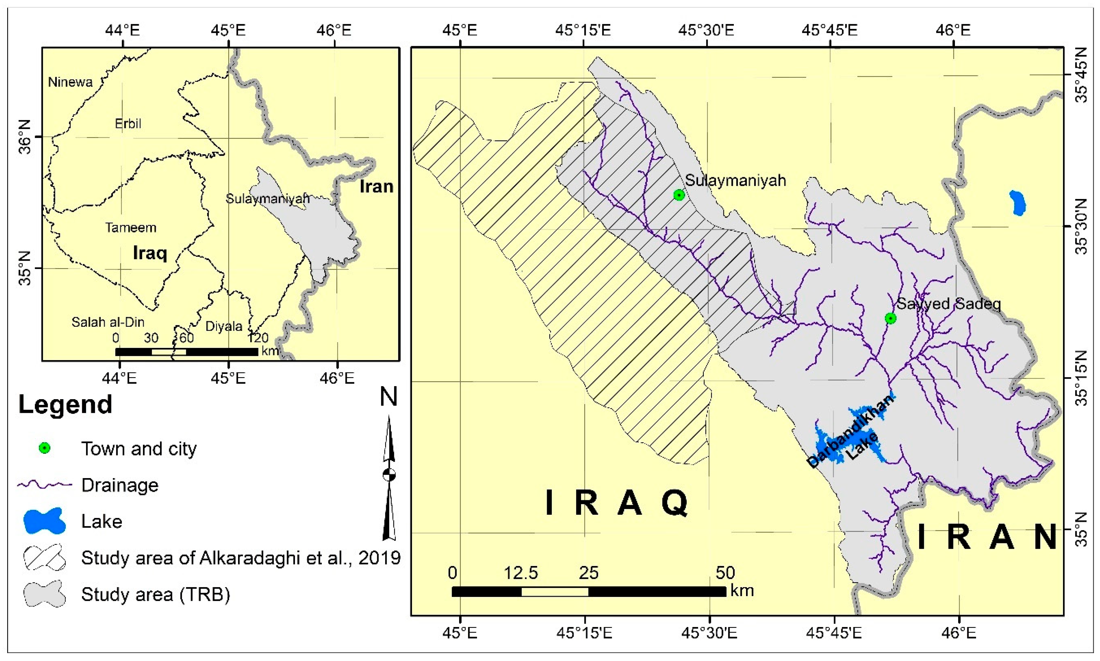
2.1. Study Area
2.2. Material
3. Predictive Factors
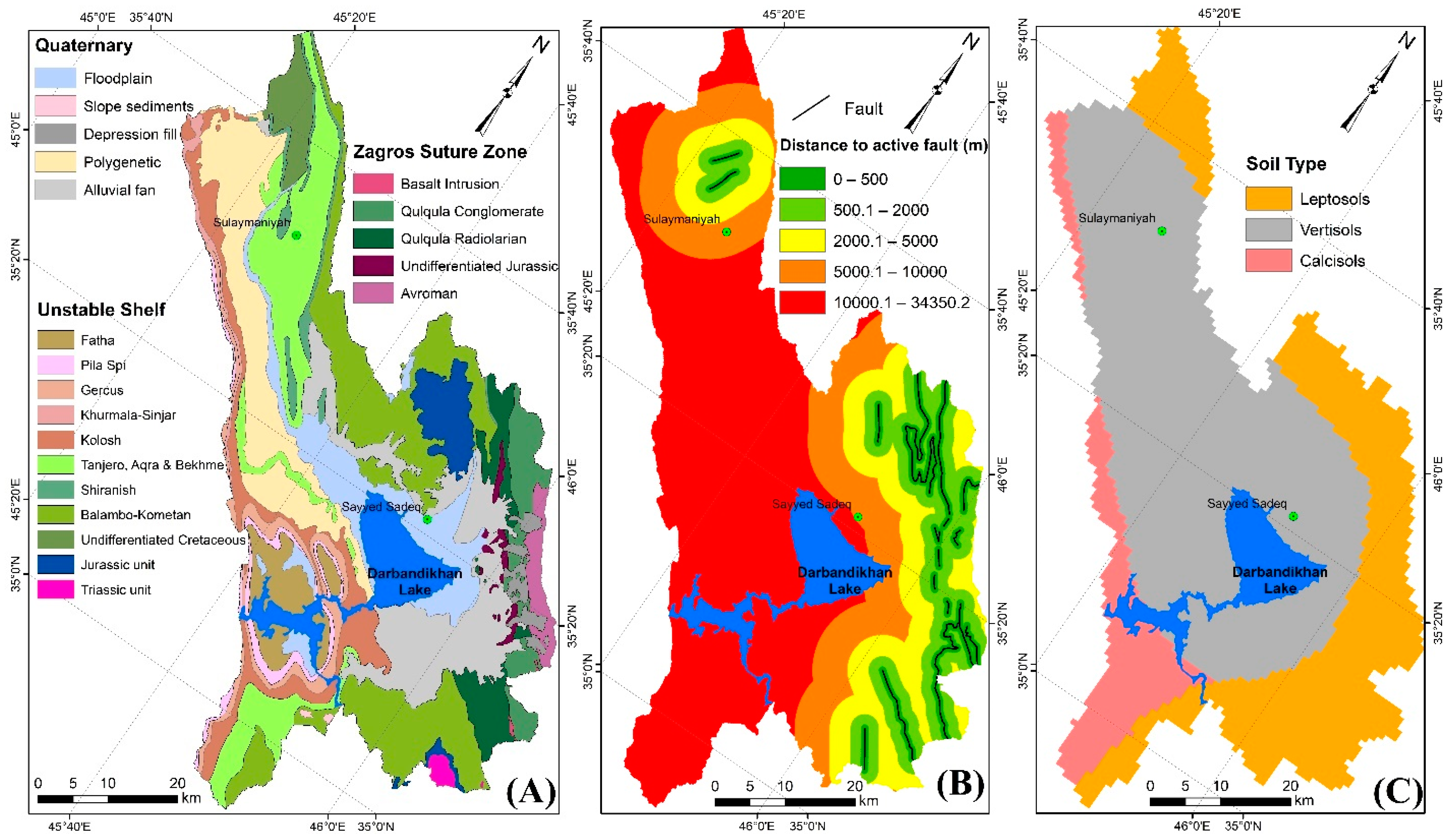
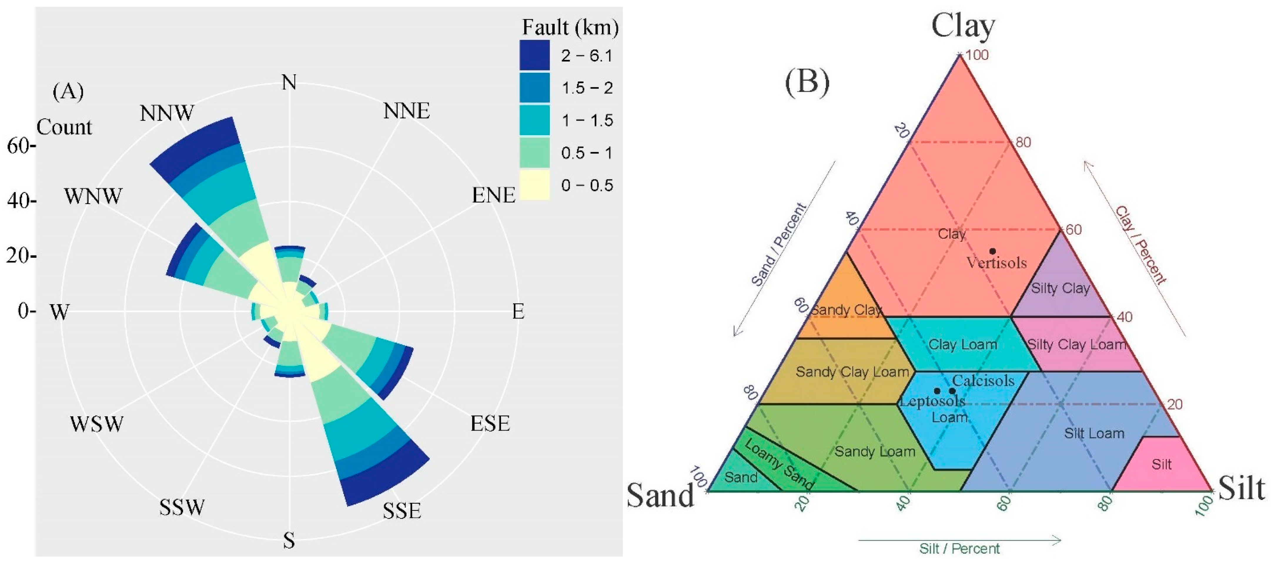
3.1. Geological Factors
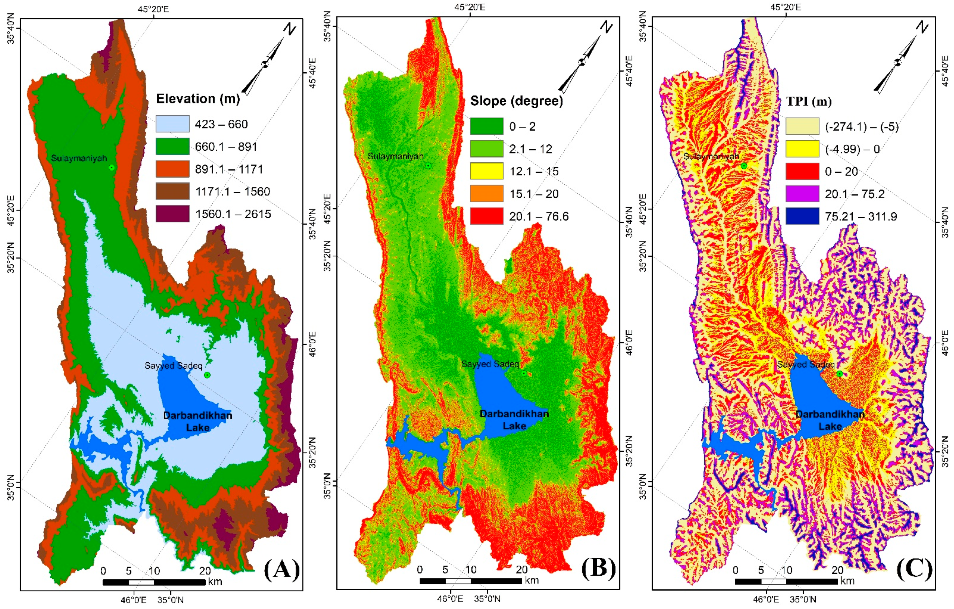
3.2. Topographic (Morphological) Factors
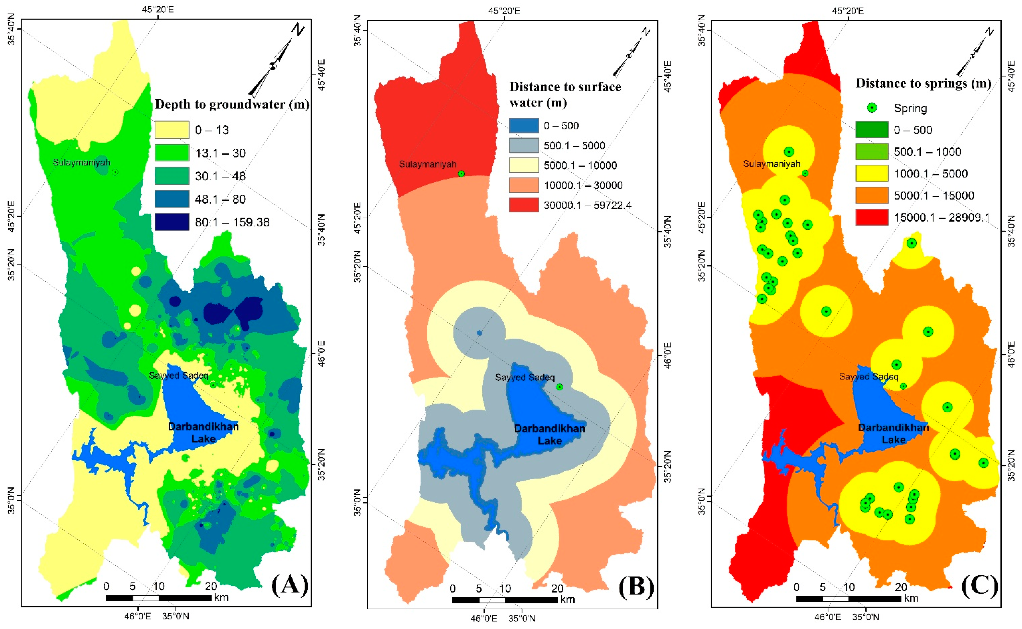
3.3. Hydrogeological and Hydrological Factors
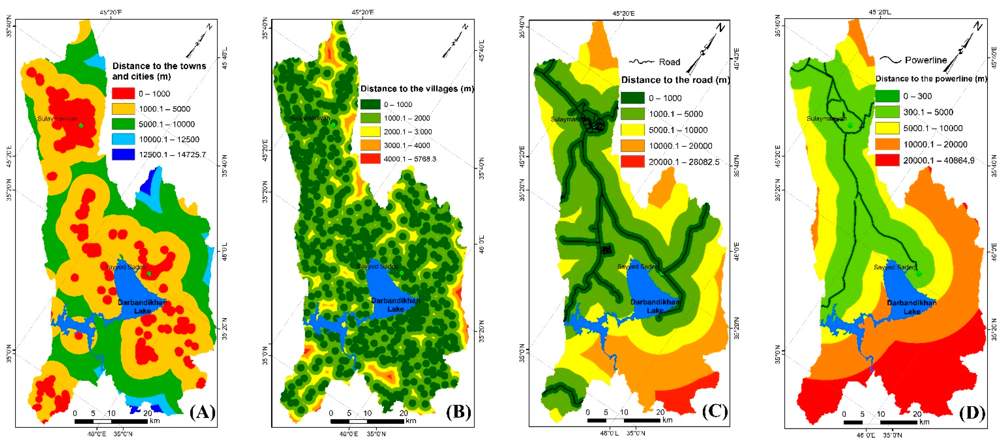
3.4. Socio-Economic Factors
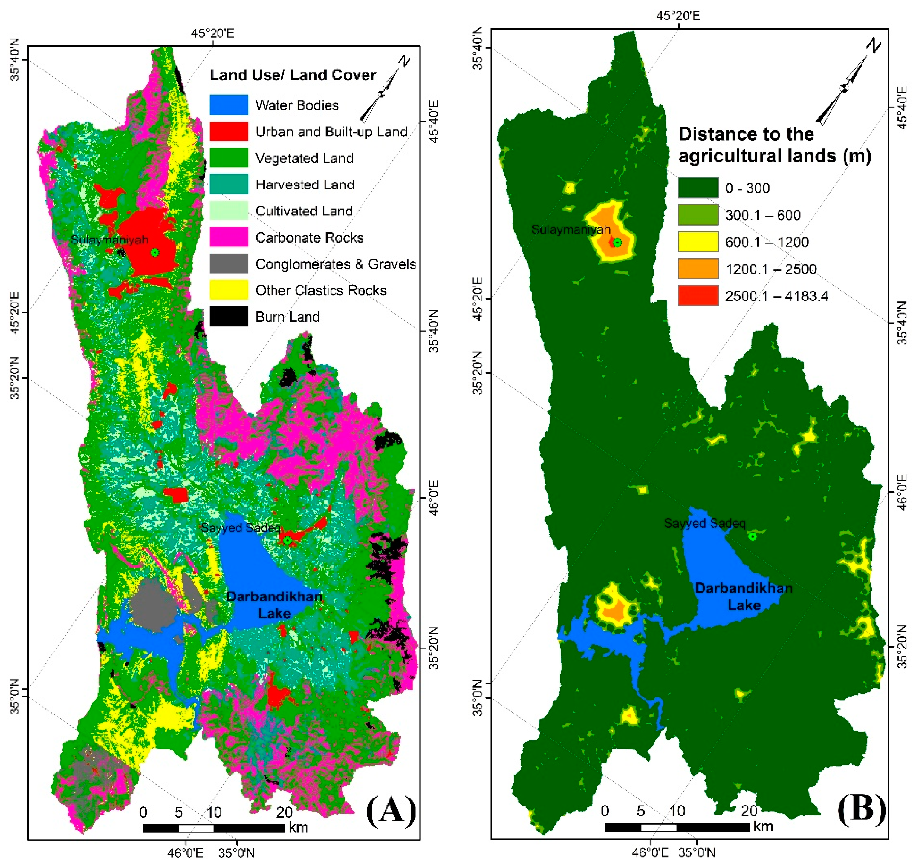
3.5. Land Use Factors
4. Suitable Landfill Site Selection Model
4.1. Boolean Overlay (BO)
4.2. Weighted Sum Method (WSM)
4.3. Weighted Product Model (WPM)
4.4. Technique for Order Performance by Similarity to an Ideal Solution (TOPSIS)
4.5. Analytic Hierarchy Process (AHP)
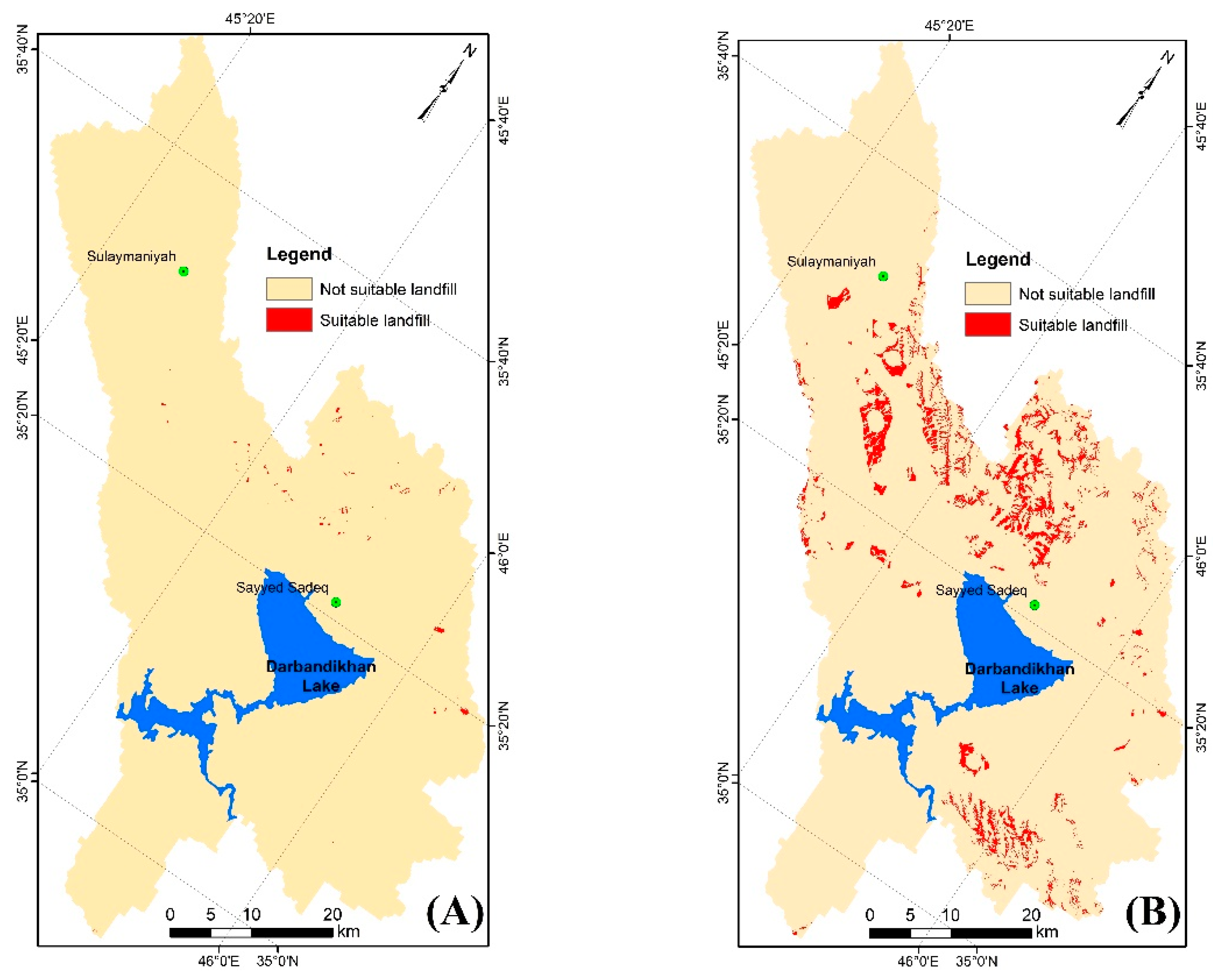
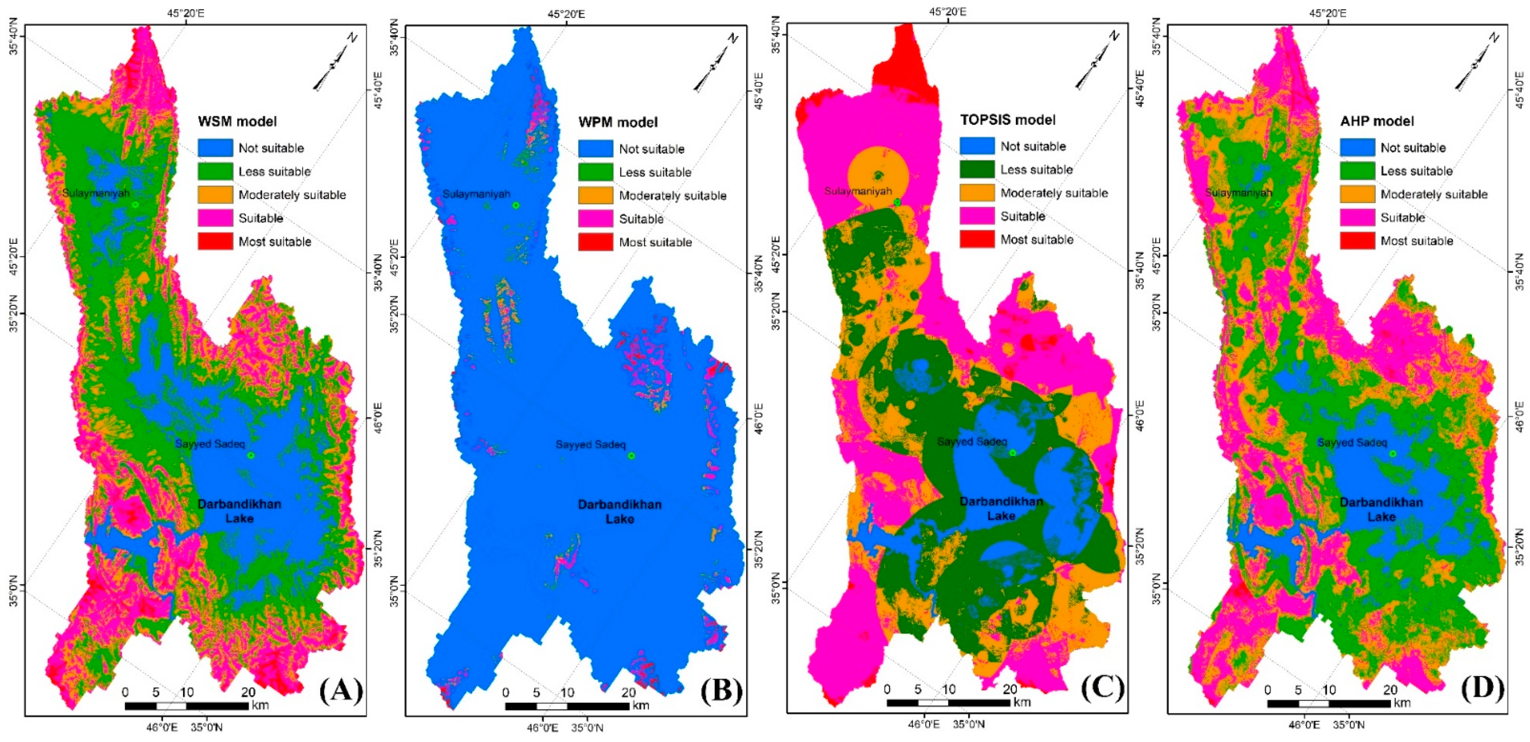
5. Results
6. Discussion
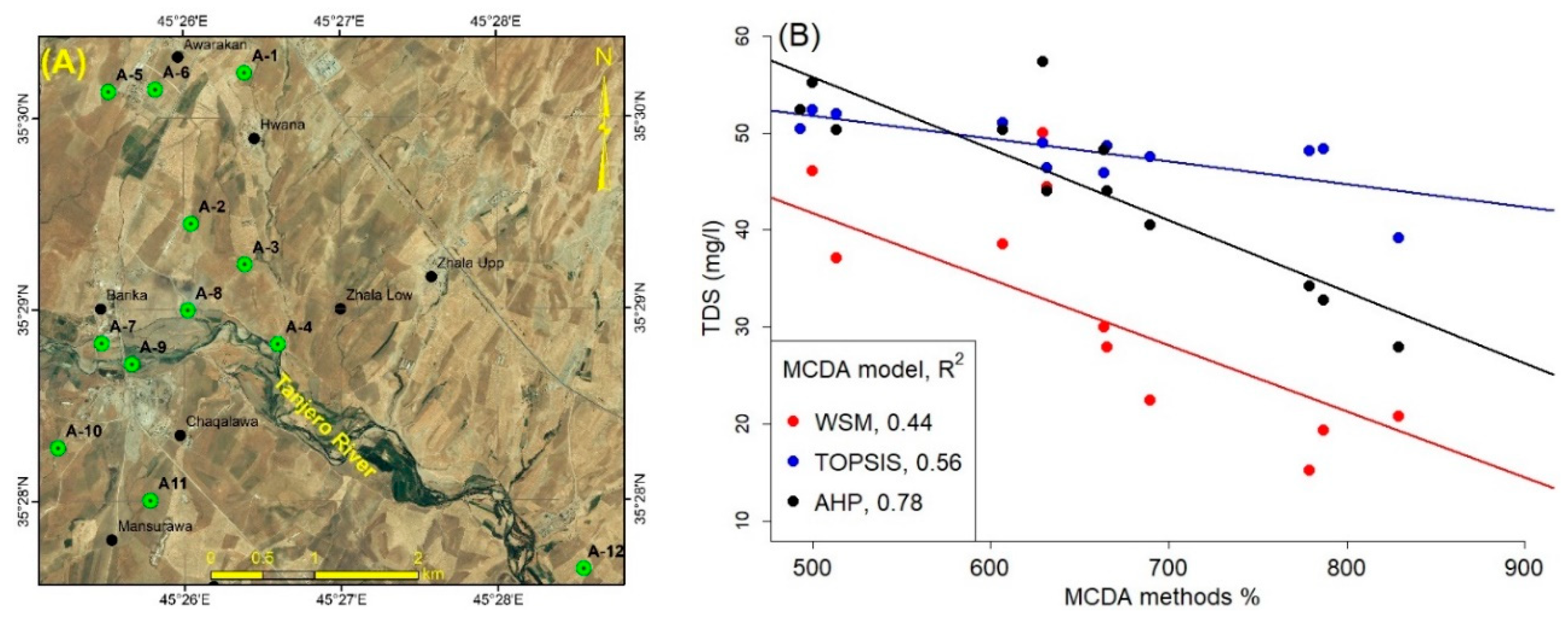
6.1. Evaluation Tanjero Landfill
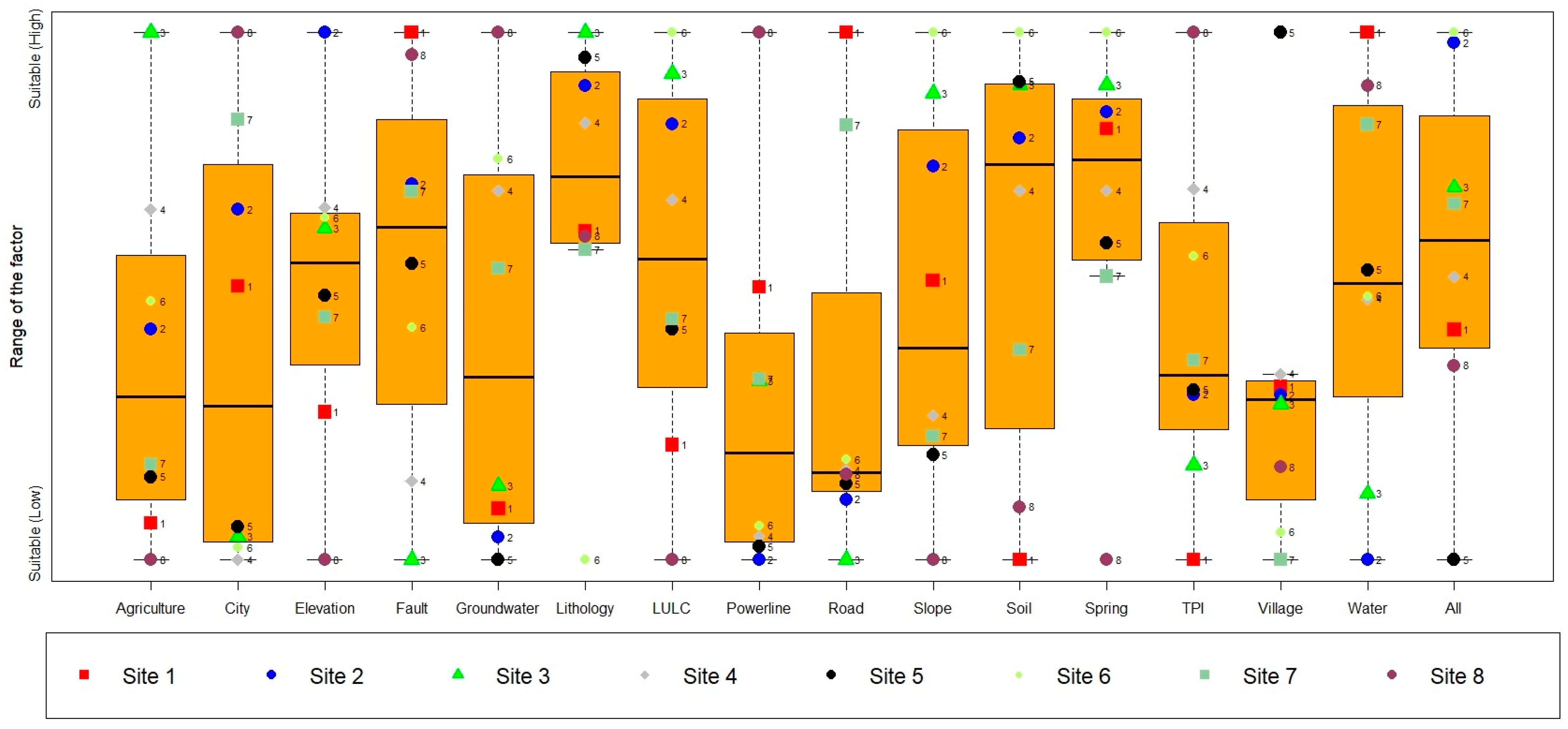
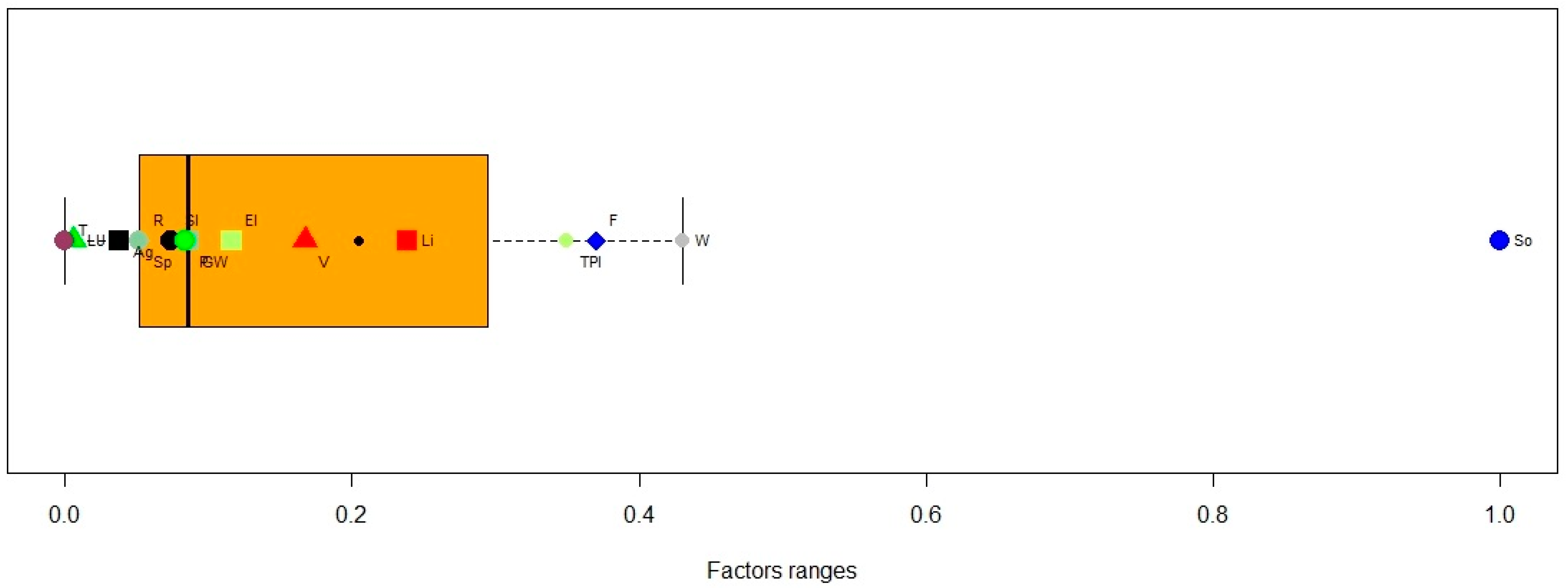
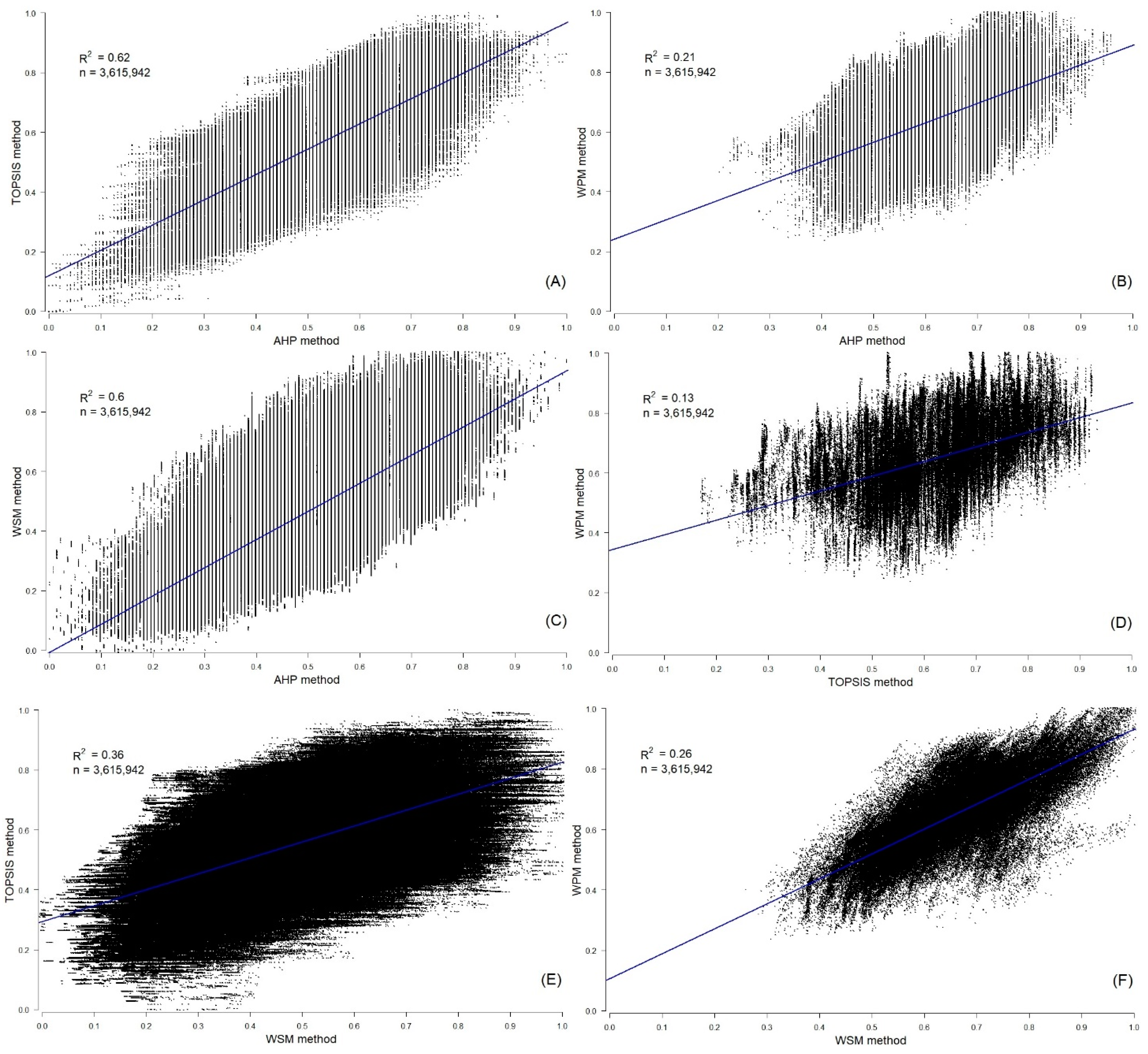
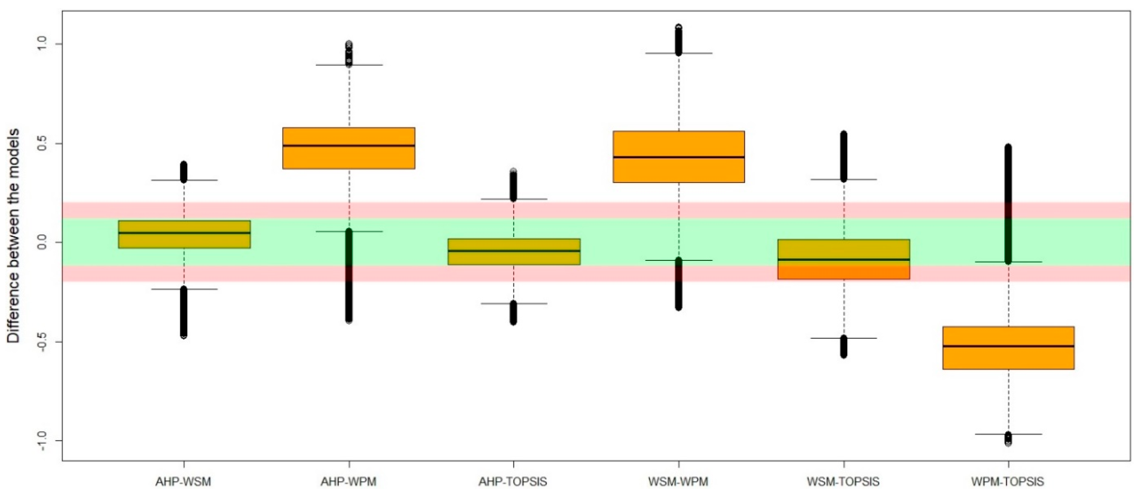
6.2. Statistical Evaluation of the MCDA Used in TRB
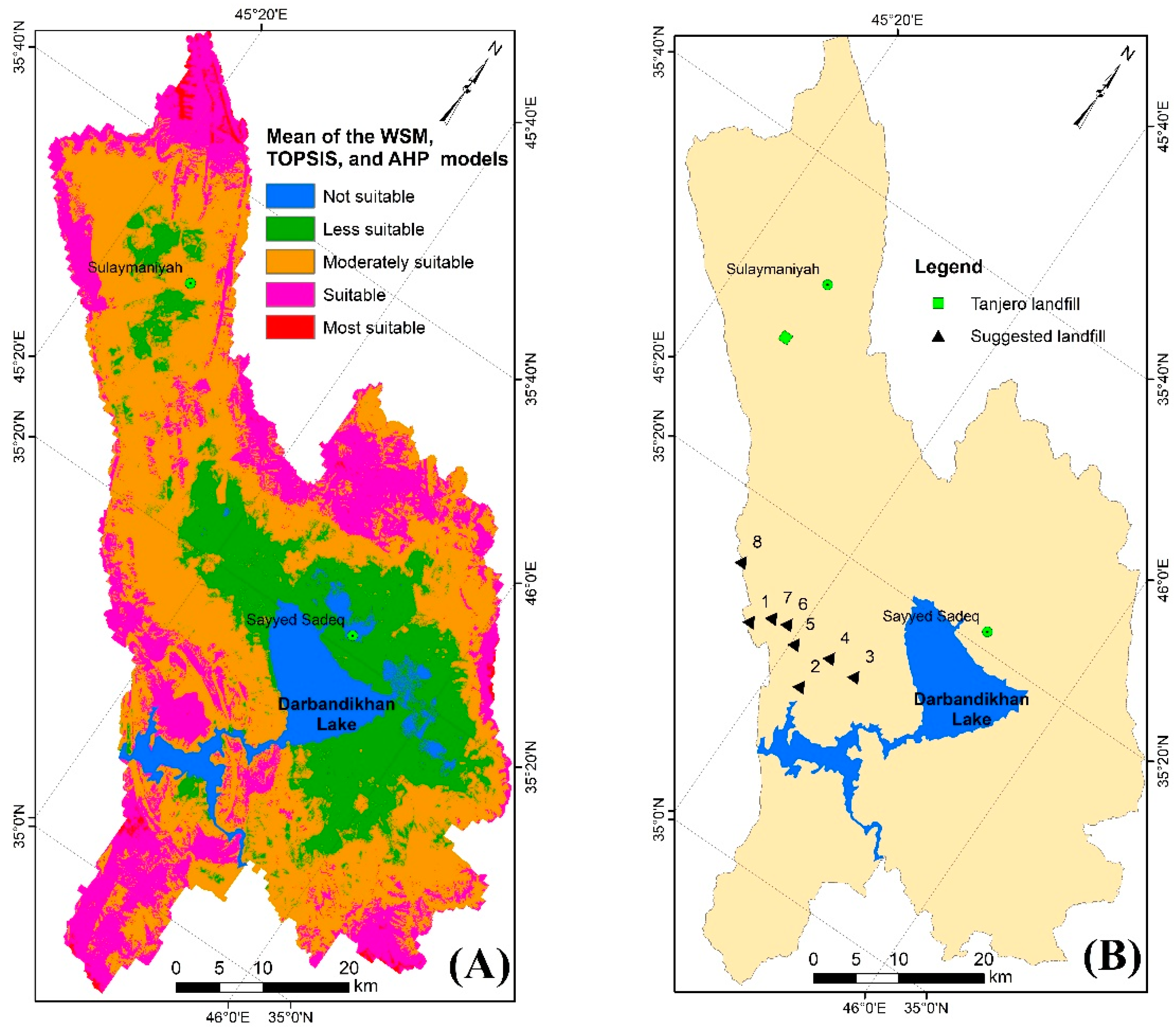
6.3. Landfill Sites Suitability
6.4. Models Validation
7. Conclusions
Author Contributions
Funding
Institutional Review Board Statement
Informed Consent Statement
Data Availability Statement
Acknowledgments
Conflicts of Interest
References
- Akintorinwa, O.J.; Okoro, O.V. Combine electrical resistivity method and multi-criteria GIS-based modeling for landfill site selection in the Southwestern Nigeria. Environ. Earth Sci. 2019, 78, 162. [Google Scholar] [CrossRef]
- Eskandari, M.; Homaee, M.; Falamaki, A. Landfill site selection for municipal solid wastes in mountainous areas with landslide susceptibility. Environ. Sci. Pollut. Res. 2016, 23, 12423–12434. [Google Scholar] [CrossRef]
- Khoshand, A.; Bafrani, A.H.; Zahedipour, M.; Mirbagheri, S.A.; Ehtehsami, M. Prevention of landfill pollution by multicriteria spatial decision support systems (MC-SDSS): Development, implementation, and case study. Environ. Sci. Pollut. Res. 2018, 25, 8415–8431. [Google Scholar] [CrossRef]
- Motlagh, Z.K.; Sayadi, M.H. Siting MSW landfills using MCE methodology in GIS environment (Case study: Birjand plain, Iran). Waste Manag. 2015, 46, 322–337. [Google Scholar] [CrossRef]
- Karimi, H.; Amiri, S.; Huang, J.; Karimi, A. Integrating GIS and multi-criteria decision analysis for landfill site selection, case study: Javanrood County in Iran. Int. J. Environ. Sci. Technol. 2018, 16, 7305–7318. [Google Scholar] [CrossRef]
- World Bank. Urban Development Overview: Development News, Research, Data; FCT Book: Washington, DC, USA, 2021. [Google Scholar]
- Zhang, R.; Yang, S.; An, Y.; Wang, Y.; Lei, Y.; Song, L. Antibiotics and antibiotic resistance genes in landfills: A review. Sci. Total Environ. 2021, 806, 150647. [Google Scholar] [CrossRef]
- Hamzeh, M.; Ali Abbaspour, R.; Davalou, R. Raster-based outranking method: A new approach for municipal solid waste landfill (MSW) siting. Environ. Sci. Pollut. Res. 2015, 22, 12511–12524. [Google Scholar] [CrossRef]
- Saaty, T.L.; Vargas, L.G. Hierarchical analysis of behavior in competition: Prediction in chess. Behav. Sci. 1980, 25, 180–191. [Google Scholar] [CrossRef]
- Hwang, C.; Yoon, K. Multiple Attribute Decision Making; Springer: Berlin, Germany, 1981. [Google Scholar]
- Fishburn, P.C. Additive Utilities with Incomplete Product Set: Applications to Priorities and Assignments. Oper. Res. 1967, 15. [Google Scholar] [CrossRef]
- Miller, D.W.; Starr, M.K. Executive Decisions and Operations Research; Prentice-Hall international Series in Management; Prentice-Hall: Hoboken, NJ, USA, 1969. [Google Scholar]
- Damasceno Pavani, I.; Ennes Cicerelli, R.; de Almeida, T.; Zandonadi Moura, L.; Contreras, F. Allocation of sanitary landfill in consortium: Strategy for the Brazilian municipalities in the State of Amazonas. Environ. Monit. Assess. 2019, 191, 39. [Google Scholar] [CrossRef]
- Ekmekçioĝlu, M.; Kaya, T.; Kahraman, C. Fuzzy multicriteria disposal method and site selection for municipal solid waste. Waste Manag. 2010, 30, 1729–1736. [Google Scholar] [CrossRef]
- Coban, A.; Ertis, I.F.; Cavdaroglu, N.A. Municipal solid waste management via multi-criteria decision making methods: A case study in Istanbul, Turkey. J. Clean. Prod. 2018, 180, 159–167. [Google Scholar] [CrossRef]
- Bah, Y.; Tsiko, R.G. Landfill site selection by integrating geographical information systems and multi-criteria decision analysis: A case study of Freetown, Sierra Leone. Afr. Geogr. Rev. 2011, 30, 67–99. [Google Scholar] [CrossRef]
- Shahabi, H.; Keihanfard, S.; Ahmad, B.B.; Amiri, M.J.T. Evaluating Boolean, AHP and WLC methods for the selection of waste landfill sites using GIS and satellite images. Environ. Earth Sci. 2014, 71, 4221–4233. [Google Scholar] [CrossRef]
- Cheng, S.; Chan, C.W.; Huang, G.H. Using multiple criteria decision analysis for supporting decisions of solid waste management. J. Environ. Sci. Health Part A Toxic/Hazard. Subst. Environ. Eng. 2002, 37, 975–990. [Google Scholar] [CrossRef]
- Alkaradaghi, K.; Ali, S.S.; Al-Ansari, N.; Laue, J.; Chabuk, A. Landfill site selection using MCDM methods and GIS in the Sulaimaniyah Governorate, Iraq. Sustainability 2019, 11, 4530. [Google Scholar] [CrossRef] [Green Version]
- Saatsaz, M.; Monsef, I.; Rahmani, M.; Ghods, A. Site suitability evaluation of an old operating landfill using AHP and GIS techniques and integrated hydrogeological and geophysical surveys. Environ. Monit. Assess. 2018, 190, 144. [Google Scholar] [CrossRef]
- Jamshidi, A.; Jahandizi, E.K.; Moshtaghie, M.; Monavari, S.M.; Tajziehchi, S.; Hashemi, A.; Jamshidi, M.; Allahgholi, L. Landfill site selection: A basis toward achieving sustainable waste management. Pol. J. Environ. Stud. 2014, 24, 1021–1029. [Google Scholar] [CrossRef]
- Bahrani, S.; Ebadi, T.; Ehsani, H.; Yousefi, H.; Maknoon, R. Modeling landfill site selection by multi-criteria decision making and fuzzy functions in GIS, case study: Shabestar, Iran. Environ. Earth Sci. 2016, 75, 337. [Google Scholar] [CrossRef]
- Bosompem, C.; Stemn, E.; Fei-Baffoe, B. Multi-criteria GIS-based siting of transfer station for municipal solid waste: The case of Kumasi Metropolitan Area, Ghana. Waste Manag. Res. 2016, 34, 1054–1063. [Google Scholar] [CrossRef]
- Chabuk, A.; Al-Ansari, N.; Hussain, H.M.; Knutsson, S.; Pusch, R. Landfill site selection using geographic information system and analytical hierarchy process: A case study Al-Hillah Qadhaa, Babylon, Iraq. Waste Manag. Res. 2016, 34, 427–437. [Google Scholar] [CrossRef] [PubMed]
- Djokanović, S.; Abolmasov, B.; Jevremović, D. GIS application for landfill site selection: A case study in Pančevo, Serbia. Bull. Eng. Geol. Environ. 2016, 75, 1273–1299. [Google Scholar] [CrossRef]
- El Maguiri, A.; Kissi, B.; Idrissi, L.; Souabi, S. Landfill site selection using GIS, remote sensing and multicriteria decision analysis: Case of the city of Mohammedia, Morocco. Bull. Eng. Geol. Environ. 2016, 75, 1301–1309. [Google Scholar] [CrossRef]
- Torabi-Kaveh, M.; Babazadeh, R.; Mohammadi, S.D.; Zaresefat, M. Landfill site selection using combination of GIS and fuzzy AHP, a case study: Iranshahr, Iran. Waste Manag. Res. 2016, 34, 438–448. [Google Scholar] [CrossRef]
- Sureshkumar, M.; Sivakumar, R.; Nagarajan, M. Selection of alternative landfill site in Kanchipuram, India by using gis and multicriteria decision analysis. Appl. Ecol. Environ. Res. 2017, 15, 627–636. [Google Scholar] [CrossRef]
- Güler, D.; Yomralıoğlu, T. Alternative suitable landfill site selection using analytic hierarchy process and geographic information systems: A case study in Istanbul. Environ. Earth Sci. 2017, 76, 678. [Google Scholar] [CrossRef]
- Rahmat, Z.G.; Niri, M.V.; Alavi, N.; Goudarzi, G.; Babaei, A.A.; Baboli, Z.; Hosseinzadeh, M. Landfill site selection using GIS and AHP: A case study: Behbahan, Iran. KSCE J. Civ. Eng. 2017, 21, 111–118. [Google Scholar] [CrossRef]
- Jamshidi-Zanjani, A.; Rezaei, M. Landfill site selection using combination of fuzzy logic and multi-attribute decision-making approach. Environ. Earth Sci. 2017, 76, 448. [Google Scholar] [CrossRef]
- Khademalhoseiny, M.S.; Ahmadi Nadoushan, M.; Radnezhad, H. Site selection for landfill gas extraction plant by fuzzy analytic hierarchy process and fuzzy analytic network process in the city of Najafabad, Iran. Energy Environ. 2017, 28, 763–774. [Google Scholar] [CrossRef]
- Kursah, M.B. Resolving the landfill siting impasse: Modelling technocratic and indigenous perspectives using GIS multicriteria approach. GeoJournal 2018, 83, 707–724. [Google Scholar] [CrossRef]
- Yildirim, V.; Memisoglu, T.; Bediroglu, S.; Colak, H.E. Municipal solid waste landfill site selection using multi-criteria decision making and gis: Case study of Bursa province. J. Environ. Eng. Landsc. Manag. 2018, 26, 107–119. [Google Scholar] [CrossRef]
- Al-Ruzouq, R.; Shanableh, A.; Omar, M.; Al-Khayyat, G. Macro and micro geo-spatial environment consideration for landfill site selection in Sharjah, United Arab Emirates. Environ. Monit. Assess. 2018, 190, 147. [Google Scholar] [CrossRef]
- Al-Anbari, M.A.; Thameer, M.Y.; Al-Ansari, N. Landfill site selection by weighted overlay technique: Case study of Al-Kufa, Iraq. Sustainability 2018, 10, 999. [Google Scholar] [CrossRef] [Green Version]
- Soroudi, M.; Omrani, G.; Moataar, F.; Jozi, S.A. Modelling an integrated fuzzy logic and multi-criteria approach for land capability assessment for optimized municipal solid waste landfill siting yeast. Pol. J. Environ. Stud. 2018, 27, 313–323. [Google Scholar] [CrossRef]
- Barakat, A.; Hilali, A.; Baghdadi, M.E.; Touhami, F. Landfill site selection with GIS-based multi-criteria evaluation technique. A case study in Béni Mellal-Khouribga Region, Morocco. Environ. Earth Sci. 2017, 76, 413. [Google Scholar] [CrossRef]
- Kapilan, S.; Elangovan, K. Potential landfill site selection for solid waste disposal using GIS and multi-criteria decision analysis (MCDA). J. Cent. South Univ. 2018, 25, 570–585. [Google Scholar] [CrossRef]
- Khodaparast, M.; Rajabi, A.M.; Edalat, A. Municipal solid waste landfill siting by using GIS and analytical hierarchy process (AHP): A case study in Qom city, Iran. Environ. Earth Sci. 2018, 77, 52. [Google Scholar] [CrossRef]
- Vosoogh, A.; Baghvand, A.; Karbassi, A.; Nasrabadi, T. Landfill site selection using pollution potential zoning of aquifers by modified DRASTIC Method: Case study in Northeast Iran. Iran. J. Sci. Technol. Trans. Civ. Eng. 2017, 41, 229–239. [Google Scholar] [CrossRef]
- Yousefi, H.; Javadzadeh, Z.; Noorollahi, Y.; Yousefi-Sahzabi, A. Landfill site selection using a multi-criteria decision-making method: A case study of the salafcheghan special economic zone, Iran. Sustainability 2018, 10, 1107. [Google Scholar] [CrossRef] [Green Version]
- Chabuk, A.J.; Al-Ansari, N.; Hussain, H.M.; Knutsson, S.; Pusch, R. GIS-based assessment of combined AHP and SAW methods for selecting suitable sites for landfill in Al-Musayiab Qadhaa, Babylon, Iraq. Environ. Earth Sci. 2017, 76, 209. [Google Scholar] [CrossRef] [Green Version]
- Directorate_of_Darbandikhan_Dam. Water-Level of Darbandikhan Reservoir; General Authority for Dams and Reservoirs: Sulaymaniyah, Iraq, 2018.
- CityPopulation Iraq: Governorates, Major Cities & Urban Centers—Population Statistics, Maps, Charts, Weather and Web Information. Available online: http://www.citypopulation.de/Iraq-Cities.html (accessed on 20 March 2021).
- Knowles, J.A. National solid waste management plan for Iraq. Waste Manag. Res. 2009, 27, 322–327. [Google Scholar] [CrossRef]
- The World Bank. The Kurdistan Region of Iraq Assessing the Economic and Social Impact of the Syrian Conflict and ISIS; United Nations: Washington, DC, USA, 2015. [Google Scholar]
- Economides, D.; Expert, W.M.; Sector, W. Local Area Development Programme in Iraq Report on Improvement Recommendations for the Waste Management Sector; UNDP: Erbil, Iraq, 2017. [Google Scholar]
- ICSSI Tanjero: The Struggle to Clean Up a Neglected River. Available online: https://www.iraqicivilsociety.org/archives/8184 (accessed on 25 November 2017).
- ESA SNAP. 2018. Available online: https://step.esa.int/main/ (accessed on 20 March 2021).
- ESRI ArcGIS. 2011. Available online: https://desktop.arcgis.com/en/ (accessed on 20 March 2021).
- Othman, A.A.; Gloaguen, R.; Andreani, L.; Rahnama, M. Improving landslide susceptibility mapping using morphometric features in the Mawat area, Kurdistan Region, NE Iraq: Comparison of different statistical models. Geomorphology 2018, 319, 147–160. [Google Scholar] [CrossRef]
- Foad, S. Tectonic Iraq Geological Survey Map of Iraq, Scale 1:1,000,000; Iraq Geological Survey: Baghdad, Iraq, 2012. [Google Scholar]
- Hamasur, G.A.; Mohammad, F.O.; Ahmed, A.J. Assessment of rock slope stability along sulaimaniyah -qaradagh main road, near Dararash Village, Sulaimaniyah, NE-Iraq. Iraqi J. Sci. 2020, 61, 3266–3286. [Google Scholar] [CrossRef]
- Othman, A.A.; Gloaguen, R. Integration of spectral, spatial and morphometric data into lithological mapping: A comparison of different Machine Learning Algorithms in the Kurdistan Region, NE Iraq. J. Asian Earth Sci. 2017, 146, 90–102. [Google Scholar] [CrossRef]
- Othman, A.A.; Gloaguen, R. Improving lithological mapping by SVM classification of spectral and morphological features: The discovery of a new chromite body in the Mawat ophiolite complex (Kurdistan, NE Iraq). Remote Sens. 2014, 6, 6867–6896. [Google Scholar] [CrossRef] [Green Version]
- Othman, A.A.; Al-Maamar, A.F.; Al-Manmi, D.A.M.; Liesenberg, V.; Hasan, S.E.; Al-Saady, Y.I.; Khwedim, K. Application of DInSAR-PSI Technology for Deformation Monitoring of the Mosul Dam, Iraq. Remote Sens. 2019, 11, 2632. [Google Scholar] [CrossRef] [Green Version]
- Othman, A.A.; Gloaguen, R. Automatic extraction and size distribution of landslides in kurdistan region, NE Iraq. Remote Sens. 2013, 5, 2389–2410. [Google Scholar] [CrossRef] [Green Version]
- Obaid, A.K.; Allen, M.B. Landscape expressions of tectonics in the Zagros fold-and-thrust belt. Tectonophysics 2019, 766, 20–30. [Google Scholar] [CrossRef]
- Ma’ala, K.A. The Geology of Sulaimaniya Quadrangle Sheet No. NI-38-3, Scale 1:250000; GEOSURV: Baghdad, Iraq, 2008. [Google Scholar]
- Barwary, A.M.; Salih, F. The Geology of Khanaqin Quadrangle, Sheet ni-38-37 (GM15), Scale 1:250000; Iraq Geological Survey: Baghdad, Iraq, 1992. [Google Scholar]
- Koc-San, D.; San, B.T.; Bakis, V.; Helvaci, M.; Eker, Z. Multi-Criteria Decision Analysis integrated with GIS and remote sensing for astronomical observatory site selection in Antalya province, Turkey. Adv. Sp. Res. 2013, 52, 39–51. [Google Scholar] [CrossRef]
- Ghobadi, M.H.; Babazadeh, R.; Bagheri, V. Siting MSW landfills by combining AHP with GIS in Hamedan province, western Iran. Environ. Earth Sci. 2013, 70, 1823–1840. [Google Scholar] [CrossRef]
- Abd-El Monsef, H. Optimization of municipal landfill siting in the Red Sea coastal desert using geographic information system, remote sensing and an analytical hierarchy process. Environ. Earth Sci. 2015, 74, 2283–2296. [Google Scholar] [CrossRef]
- Nachtergaele, F.; van Velthuizen, H.; van Engelen, V.; Fischer, G.; Jones, A.; Montanarella, L.; Petri, M.; Prieler, S.; Teixeira, E.; Shi, X. Harmonized World Soil Database, version 1.2; FAO: Rome, Italy; IIASA: Laxenburg; Austria, 2012; pp. 1–50. [Google Scholar]
- Kara, C.; Doratli, N. Application of GIS/AHP in siting sanitary landfill: A case study in Northern Cyprus. Waste Manag. Res. 2012, 30, 966–980. [Google Scholar] [CrossRef]
- Kumar, A.; Pinto, M.C.; Candeias, C.; Dinis, P.A. Baseline maps of potentially toxic elements in the soils of Garhwal Himalayas, India: Assessment of their eco-environmental and human health risks. Land Degrad. Dev. 2021, 32, 3856–3869. [Google Scholar] [CrossRef]
- Kumar, A.; Kumar, M.; Pandey, R.; ZhiGuo, Y.; Cabral-Pinto, M. Forest soil nutrient stocks along altitudinal range of Uttarakhand Himalayas: An aid to Nature Based Climate Solutions. CATENA 2021, 207, 105667. [Google Scholar] [CrossRef]
- USDA. Soil Mechanics Level 1, Module 3. USDA Textural Classification Study Guide; United States Department of Agriculture: Washington, DC, USA, 1987.
- Demesouka, O.E.; Vavatsikos, A.P.; Anagnostopoulos, K.P. GIS-based multicriteria municipal solid waste landfill suitability analysis: A review of the methodologies performed and criteria implemented. Waste Manag. Res. 2014, 32, 270–296. [Google Scholar] [CrossRef]
- Demesouka, O.E.; Vavatsikos, A.P.; Anagnostopoulos, K.P. Suitability analysis for siting MSW landfills and its multicriteria spatial decision support system: Method, implementation and case study. Waste Manag. 2013, 33, 1190–1206. [Google Scholar] [CrossRef] [PubMed]
- Charnpratheep, K.; Zhou, Q.; Garner, B. Preliminary landfill site screening using fuzzy geographical information systems. Waste Manag. Res. 1997, 15, 197–215. [Google Scholar] [CrossRef]
- Ersoy, H.; Bulut, F. Spatial and multi-criteria decision analysis-based methodology for landfill site selection in growing urban regions. Waste Manag. Res. 2009, 27, 489–500. [Google Scholar] [CrossRef]
- Weiss, A.D. Topographic position and landforms analysis. In Proceedings of the ESRI Users Conference, San Diego, CA, USA, 9–13 July 2001. [Google Scholar]
- ESRI. ArcGIS Help Library; ESRI: West Redlands, CA, USA, 2012. [Google Scholar]
- Abd-El Monsef, H.; Smith, S.E. Integrating remote sensing, geographic information system, and analytical hierarchy process for hazardous waste landfill site selection. Arab. J. Geosci. 2019, 12, 155. [Google Scholar] [CrossRef]
- Sulaymaniyah Groundwater Directorate (SGD). Borehole Data and Water Level Information; SGD: Sulaymaniyah, Iraq, 2018. [Google Scholar]
- Mustafa, O.M. Impact of Sewage Waste Water on the Environment of Tanjero River and its Basin within Sulaimani City/NE-Iraq; University of Baghdad: Baghdad, Iraq, 2006. [Google Scholar]
- Al-hasnawi, S.S. Water Quality Index Of Tanjero River Basin Near Sulaymania City. Al-Mustansiriyah J. Sci. Res. 2012, 23, 193–200. [Google Scholar]
- Aziz, N.A. Pollution of Tanjero River by Some Heavy Metals Generated from Sewage Wastwater and Industrial Wastewater in Sulaimani District. J. Kirkuk Univ.-Sci. Stud. 2012, 7, 67–84. [Google Scholar] [CrossRef]
- Kareem, A.; Mustafa, O.; Merkel, B. Geochemical and environmental investigation of the water resources of the Tanjero area, Kurdistan region, Iraq. Arab. J. Geosci. 2018, 11, 461. [Google Scholar] [CrossRef]
- Khwakaram, A.I. On water quality of qalyasan stream, tanjero river and impact of fat, oil and grease on darbandikhan reservoir in Sulaimani City-Kurdistan Region of Iraq-Iraq. Int. J. Environ. Ecol. Fam. Urban Stud. 2016, 6, 1–12. [Google Scholar]
- Hamamin, D.F.; Qadir, R.A.; Ali, S.S. Groundwater vulnerability map of Sulaymaniyah sub-basin using SINTACS model, Sulaymaniyah Governorate, Kurdistan Region, Iraq. J. Zankoy Sulaimani Part-A Pure Appl. Sci. 2016, 277–292. [Google Scholar] [CrossRef]
- Othman, N.; Kane, T.; Hawrami, K.M.; Alkaradaghi, K.; Salih, F.A.; Khwa, K.; Hamafaraj, R.; Ali, T. Assessing health risks to local population from contamination sources in and around Sulaimani province; a qualitative study. J. Zankoy Sulaimani Part-A Pure Appl. Sci. 2018, 20, 45–62. [Google Scholar] [CrossRef]
- Şener, Ş.; Sener, E.; Karagüzel, R. Solid waste disposal site selection with GIS and AHP methodology: A case study in Senirkent–Uluborlu (Isparta) Basin, Turkey. Environ. Monit. Assess. 2011, 173, 533–554. [Google Scholar] [CrossRef]
- Rasul, A.K. Hydrochemistry and quality assessment of Derbendikhan Reservoir, Kurdistan Region, Northeastern Iraq. Arab. J. Geosci. 2019, 12, 312. [Google Scholar] [CrossRef]
- SSWD. Sulaymaniyah Surface Water Directorate; Spring Data; SSWD: Sulaymaniyah, Iraq, 2018. [Google Scholar]
- Isalou, A.A.; Zamani, V.; Shahmoradi, B.; Alizadeh, H. Landfill site selection using integrated fuzzy logic and analytic network process (F-ANP). Environ. Earth Sci. 2013, 68, 1745–1755. [Google Scholar] [CrossRef]
- Kontos, T.D.; Komilis, D.P.; Halvadakis, C.P. Siting MSW landfills on Lesvos island with a GIS-based methodology. Waste Manag. Res. 2003, 21, 262–277. [Google Scholar] [CrossRef]
- Kao, J.-J.; Lin, H.-Y. Multifactor spatial analysis for landfill siting. J. Environ. Eng. 1996, 122, 902–908. [Google Scholar] [CrossRef] [Green Version]
- OCHA-IRAQ Iraq—Datasets 2018. Available online: www.unocha.org/iraq/about-ocha-iraq (accessed on 27 February 2021).
- Al-Rubaiay, A.T.; Al-Dulaimi, T.Y. Series of Land Use Land Cover Maps of Iraq Scale 1:250 000, Sulaimaniya Quadrangle Sheet NI–38–3 (LULCM 10); GEOSURV: Baghdad, Iraq, 2012. [Google Scholar]
- Sai Krishna, V.V.; Pandey, K.; Karnatak, H. Geospatial multicriteria approach for solid waste disposal site selection in Dehradun city, India. Curr. Sci. 2017, 112, 549–559. [Google Scholar] [CrossRef]
- Rouse, J.W.; Haas, R.H.; Schelle, J.A.; Deering, D.W.; NASA/GSFC. Monitoring the Vernal Advancement or Retrogradation of Natural Vegetation; NASA: Greenbelt, MD, USA, 1974.
- Mulliner, E.; Malys, N.; Maliene, V. Comparative analysis of MCDM methods for the assessment of sustainable housing affordability. Omega 2016, 59, 146–156. [Google Scholar] [CrossRef]
- Guitouni, A.; Martel, J.-M. Tentative guidelines to help choosing an appropriate MCDA method. Eur. J. Oper. Res. 1998, 109, 501–521. [Google Scholar] [CrossRef]
- Roy, B.; Słowiński, R. Questions guiding the choice of a multicriteria decision aiding method. EURO J. Decis. Process. 2013, 1, 69–97. [Google Scholar] [CrossRef] [Green Version]
- Triantaphyllou, E. Multi-Criteria Decision Making Methods: A Comparative Study; Applied Optimization; Springer: Berlin/Heidelberg, Germany, 2000; ISBN 9780792366072. [Google Scholar]
- Hwang, C.L.; Yoon, K. Multiple Attribute Decision Making: Methods and Applications A State-of-the-Art Survey; Lecture Notes in Economics and Mathematical Systems; Springer: Berlin/Heidelberg, Germany, 2012; ISBN 9783642483189. [Google Scholar]
- Milillo, P.; Perissin, D.; Salzer, J.T.; Lundgren, P.; Lacava, G.; Milillo, G.; Serio, C. Monitoring dam structural health from space: Insights from novel InSAR techniques and multi-parametric modeling applied to the Pertusillo dam Basilicata, Italy. Int. J. Appl. Earth Obs. Geoinf. 2016, 52, 221–229. [Google Scholar] [CrossRef]
- Afzali, A.; Sabri, S.; Rashid, M.; Mohammad Vali Samani, J.; Ludin, A.N.M. Inter-Municipal Landfill Site Selection Using Analytic Network Process. Water Resour. Manag. 2014, 28, 2179–2194. [Google Scholar] [CrossRef]
- Baiocchi, V.; Lelo, K.; Polettini, A.; Pomi, R. Land suitability for waste disposal in metropolitan areas. Waste Manag. Res. 2014, 32, 707–716. [Google Scholar] [CrossRef]
- Delgado, O.B.; Mendoza, M.; Granados, E.L.; Geneletti, D. Analysis of land suitability for the siting of inter-municipal landfills in the Cuitzeo Lake Basin, Mexico. Waste Manag. 2008, 28, 1137–1146. [Google Scholar] [CrossRef]
- Lin, H.-Y.; Kao, J.-J. Grid-based heuristic method for multifactor landfill siting. J. Comput. Civ. Eng. 2005, 19, 369–376. [Google Scholar] [CrossRef]
- Islam, A.; Ali, S.M.; Afzaal, M.; Iqbal, S.; Zaidi, S.N.F. Landfill sites selection through analytical hierarchy process for twin cities of Islamabad and Rawalpindi, Pakistan. Environ. Earth Sci. 2018, 77, 72. [Google Scholar] [CrossRef]
- Sizirici, B.; Tansel, B.; Kumar, V. Knowledge based ranking algorithm for comparative assessment of post-closure care needs of closed landfills. Waste Manag. 2011, 31, 1232–1238. [Google Scholar] [CrossRef] [PubMed]
- Othman, A.A.; Al-Maamar, A.F.; Al-Manmi, D.A.M.; Veraldo, L.; Hasan, S.E.; Obaid, A.K.; Al-Quraishi, A.M.F. GIS-based modeling for selection of dam sites in the Kurdistan Region, Iraq. ISPRS Int. J. Geo-Inf. 2020, 9, 244. [Google Scholar] [CrossRef] [Green Version]
- Bellehumeur, C.; Vasseur, L.; Ansseau, C.; Marcos, B. Implementation of a multicriteria sewage sludge management model in the southern Quebec municipality of Lac-Megantic, Canada. J. Environ. Manag. 1997, 50, 51–66. [Google Scholar] [CrossRef]
- Daghouri, A.; Mansouri, K.; Qbadou, M. Multi criteria decision making methods for information system selection: A comparative study. In Proceedings of the 2018 International Conference on Electronics, Control, Optimization and Computer Science, ICECOCS 2018, Kenitra, Morocco, 5–6 December 2018. [Google Scholar]
- Chakraborty, S.; Zavadskas, E.K.; Antucheviciene, J. Applications of WASPAS method as a multi-criteria decision-making tool. Econ. Comput. Econ. Cybern. Stud. Res. 2015, 49, 5–22. [Google Scholar]
- Yal, G.P.; Akgün, H. Landfill site selection and landfill liner design for Ankara, Turkey. Environ. Earth Sci. 2013, 70, 2729–2752. [Google Scholar] [CrossRef]
- Mokhtarian, M.N.; Sadi-Nezhad, S.; Makui, A. A new flexible and reliable IVF-TOPSIS method based on uncertainty risk reduction in decision making process. Appl. Soft Comput. J. 2014, 23, 509–520. [Google Scholar] [CrossRef]
- Aghajani Mir, M.; Taherei Ghazvinei, P.; Sulaiman, N.M.N.; Basri, N.E.A.; Saheri, S.; Mahmood, N.Z.; Jahan, A.; Begum, R.A.; Aghamohammadi, N. Application of TOPSIS and VIKOR improved versions in a multi criteria decision analysis to develop an optimized municipal solid waste management model. J. Environ. Manag. 2016, 166, 109–115. [Google Scholar] [CrossRef]
- Akbaş, H.; Bilgen, B. An integrated fuzzy QFD and TOPSIS methodology for choosing the ideal gas fuel at WWTPs. Energy 2017, 125, 484–497. [Google Scholar] [CrossRef]
- Sabaghi, M.; Mascle, C.; Baptiste, P. Evaluation of products at design phase for an efficient disassembly at end-of-life. J. Clean. Prod. 2016, 116, 177–186. [Google Scholar] [CrossRef]
- Maimoun, M.; Madani, K.; Reinhart, D. Multi-level multi-criteria analysis of alternative fuels for waste collection vehicles in the United States. Sci. Total Environ. 2016, 550, 349–361. [Google Scholar] [CrossRef] [Green Version]
- Avikal, S.; Jain, R.; Mishra, P.K. A Kano model, AHP and M-TOPSIS method-based technique for disassembly line balancing under fuzzy environment. Appl. Soft Comput. J. 2014, 25, 519–529. [Google Scholar] [CrossRef]
- Asefi, H.; Lim, S. A novel multi-dimensional modeling approach to integrated municipal solid waste management. J. Clean. Prod. 2017, 166, 1131–1143. [Google Scholar] [CrossRef]
- Li, J.; Yang, Y.; Huan, H.; Li, M.; Xi, B.; Lv, N.; Wu, Y.; Xie, Y.; Li, X.; Yang, J. Method for screening prevention and control measures and technologies based on groundwater pollution intensity assessment. Sci. Total Environ. 2016, 551–552, 143–154. [Google Scholar] [CrossRef] [PubMed]
- Yıldırım, Ü.; Güler, C. Identification of suitable future municipal solid waste disposal sites for the Metropolitan Mersin (SE Turkey) using AHP and GIS techniques. Environ. Earth Sci. 2016, 75, 101. [Google Scholar] [CrossRef]
- De Felicori, T.C.; Marques, E.A.G. Multicriteria decision analysis applied in the selection of suitable areas for disposal of solid waste in Zona da Mata, Minas Gerais, Brazil. J. Solid Waste Technol. Manag. 2017, 43, 47–64. [Google Scholar] [CrossRef]
- Aksoy, E.; San, B.T. Geographical information systems (GIS) and Multi-Criteria Decision Analysis (MCDA) integration for sustainable landfill site selection considering dynamic data source. Bull. Eng. Geol. Environ. 2019, 78, 779–791. [Google Scholar] [CrossRef]
- Saaty, T.L. The Analytic Hierarchy Process in Conflict Management. Int. J. Confl. Manag. 1990, 1, 47–68. [Google Scholar] [CrossRef]
- Zhang, L.; Lavagnolo, M.C.; Bai, H.; Pivato, A.; Raga, R.; Yue, D. Environmental and economic assessment of leachate concentrate treatment technologies using analytic hierarchy process. Resour. Conserv. Recycl. 2019, 141, 474–480. [Google Scholar] [CrossRef]
- Salar, S.G.; Othman, A.A.; Hasan, S.E. Identification of suitable sites for groundwater recharge in Awaspi watershed using GIS and remote sensing techniques. Environ. Earth Sci. 2018, 77, 701. [Google Scholar] [CrossRef]
- Liang, H.; He, S.; Lei, X.; Bi, Y.; Liu, W.; Ouyang, C. Dynamic process simulation of construction solid waste (CSW) landfill landslide based on SPH considering dilatancy effects. Bull. Eng. Geol. Environ. 2019, 78, 763–777. [Google Scholar] [CrossRef]
- Xiu, W.; Wang, S.; Qi, W.; Li, X.; Wang, C. Disaster Chain Analysis of Landfill Landslide: Scenario Simulation and Chain-Cutting Modeling. Sustainability 2021, 13, 5032. [Google Scholar] [CrossRef]
- Lei, W.; Xiaoguang, C.; Ping, L.; Yuna, Q. Numerical analysis of dynamic characteristics of sludge-type slag landfill landslide. In Proceedings of the IOP Conference Series: Earth and Environmental Science, Virtual, China, 23–29 November 2021; Volume 676. [Google Scholar] [CrossRef]
- Bera, A.; Mukhopadhyay, B.P.; Chowdhury, P.; Ghosh, A.; Biswas, S. Groundwater vulnerability assessment using GIS-based DRASTIC model in Nangasai River Basin, India with special emphasis on agricultural contamination. Ecotoxicol. Environ. Saf. 2021, 214, 112085. [Google Scholar] [CrossRef] [PubMed]
- Le, T.N.; Tran, D.X.; Tran, T.V.; Gyeltshen, S.; Lam, T.V.; Luu, T.H.; Nguyen, D.Q.; Dao, T. V Estimating soil water susceptibility to salinization in the mekong river delta using a modified drastic model. Water 2021, 13, 1636. [Google Scholar] [CrossRef]

| Reference | Slope (%) | Residential Areas (m) | Roads (m) | Surface Waters (m) | Lithology | LULC | Groundwater Depth (m) | Village | Airport and Religious (Protected Area) | Soil | Topography | Fault (m) | Powerlines (m) | Spring | Historical sites | Orchards and Agricultural Lands (m) | Aspect | Railways | Oil and Gas Pipelines | Industries (m) | Floodway (m) | Rainfall | Mine | Erosion | Sensitive Ecosystems | Population/km–2 | Wind | Temperature | Drainage Density | Geomorphology |
|---|---|---|---|---|---|---|---|---|---|---|---|---|---|---|---|---|---|---|---|---|---|---|---|---|---|---|---|---|---|---|
| [2] | * | * | * | * | * | * | * | * | * | * | * | * | * | * | * | |||||||||||||||
| [3] | * | * | * | * | * | * | * | * | * | * | * | * | * | |||||||||||||||||
| [19] | * | * | * | * | * | * | * | * | * | * | * | * | * | |||||||||||||||||
| [20] | * | * | * | * | * | * | * | * | * | * | * | |||||||||||||||||||
| [21] | * | * | * | * | * | * | * | * | * | * | * | * | * | |||||||||||||||||
| [22] | * | * | * | * | * | * | * | * | * | * | * | * | * | * | * | |||||||||||||||
| [23] | * | * | * | * | * | * | * | |||||||||||||||||||||||
| [24] | * | * | * | * | * | * | * | * | * | * | * | * | * | |||||||||||||||||
| [25] | * | * | * | * | * | * | * | * | * | * | * | * | * | |||||||||||||||||
| [26] | * | * | * | * | * | |||||||||||||||||||||||||
| [27] | * | * | * | * | * | * | * | * | * | |||||||||||||||||||||
| [28] | * | * | * | * | * | * | ||||||||||||||||||||||||
| [29] | * | * | * | * | * | * | * | * | ||||||||||||||||||||||
| [30] | * | * | * | * | * | * | * | * | * | |||||||||||||||||||||
| [31] | * | * | * | * | * | * | * | * | * | * | * | * | ||||||||||||||||||
| [32] | * | * | * | * | * | * | * | * | * | |||||||||||||||||||||
| [33] | * | * | * | * | * | * | * | * | * | * | ||||||||||||||||||||
| [34] | * | * | * | * | * | * | * | * | * | * | * | |||||||||||||||||||
| [35] | * | * | * | * | * | * | * | * | ||||||||||||||||||||||
| [36] | * | * | * | * | * | * | * | * | * | |||||||||||||||||||||
| [37] | * | * | * | * | * | * | * | * | * | * | * | * | * | * | * | * | ||||||||||||||
| [38] | * | * | * | * | * | * | * | * | * | * | ||||||||||||||||||||
| [39] | * | * | * | * | * | * | * | * | * | |||||||||||||||||||||
| [40] | * | * | * | * | * | * | * | * | * | * | * | |||||||||||||||||||
| [41] | * | * | * | * | * | * | ||||||||||||||||||||||||
| [42] | * | * | * | * | * | * | * | * | * | * | ||||||||||||||||||||
| [43] | * | * | * | * | * | * | * | * | * | * | * | * | * | * | ||||||||||||||||
| Average rate | 85.2 | 85.2 | 81.5 | 74.1 | 66.7 | 66.7 | 63 | 63 | 51.9 | 51.9 | 48.2 | 40.7 | 33.3 | 29.6 | 25.9 | 25.9 | 22.2 | 22.2 | 14.8 | 11.1 | 7.4 | 7.4 | 7.4 | 7.4 | 7.4 | 7.4 | 7.4 | 3.7 | 3.7 | 3.7 |
| No | Factor | Relationship Type | Type of Data | Relation Intensity |
|---|---|---|---|---|
| 1 | Lithology | No relation | Discrete | Strong |
| 2 | Soil | No relation | Discrete | Weak |
| 3 | LULC | No relation | Discrete | Weak |
| 4 | Distance to road | No relation | Discrete | Weak |
| 5 | Slope (°) | No relation | Continuous | Weak |
| 6 | TPI | No relation | Discrete | Very weak |
| 7 | Groundwater depth (m) | Direct | Continuous | Strong |
| 8 | Distance to towns and cities (m) | Direct | Continuous | Strong |
| 9 | Distance to village (m) | Direct | Continuous | Strong |
| 10 | Distance to active fault (m) | Direct | Continuous | Moderate |
| 11 | Distance to Powerline (m) | Direct | Continuous | Weak |
| 12 | Distance to surface water bodies (m) | Direct | Continuous | Very strong |
| 13 | Distance to agricultural lands (m) | Direct | Continuous | Weak |
| 14 | Elevation | No relation | Continuous | Weak |
| 15 | Distance to springs | Direct | Continuous | Very weak |
| Lithology | Suitability | Rank | Normalized Weight | Groundwater Depth (m) | Suitability | Rank | Normalized Weight |
|---|---|---|---|---|---|---|---|
| Lake | Not suitable | 1 | 0.00317 | 0–13 | Not suitable | 1 | 0.003623 |
| Floodplain | Not suitable | 1 | 0.00317 | 13.1–30 | Less suitable | 3 | 0.01087 |
| Slope sediments | Not suitable | 1 | 0.00317 | 30.1–48 | Moderately suitable | 5 | 0.018116 |
| Depression fill | Not suitable | 1 | 0.00317 | 48.1–80 | Suitable | 7 | 0.025362 |
| Polygenetic sediments | Not suitable | 1 | 0.00317 | 80.1–159.38 | Most suitable | 9 | 0.032609 |
| Alluvial fan | Not suitable | 1 | 0.00317 | Distance to Towns and Cities (m) | Suitability | Rank | Normalized Weight |
| Avroman limestone | Less suitable | 3 | 0.009511 | 0–1000 | Not suitable | 1 | 0.00317 |
| Undifferentiated Jurassic | Moderately suitable | 5 | 0.015851 | 1000.1–5000 | Less suitable | 3 | 0.009511 |
| Qulqula radiolarian | Not suitable | 1 | 0.00317 | 5000.1–10,000 | Moderately suitable | 5 | 0.015851 |
| Qulqula conglomerate | Less suitable | 3 | 0.009511 | 10,000.1–20,000 | Suitable | 7 | 0.022192 |
| Basalt intrusion | Most suitable | 9 | 0.028533 | 20,000.1–14,725.7 | Most suitable | 9 | 0.028533 |
| Fatha | Most suitable | 9 | 0.028533 | Distance to Village (m) | Suitability | Rank | Normalized Weight |
| Pila Spi | Less suitable | 3 | 0.009511 | 0–1000 | Not suitable | 1 | 0.00317 |
| Gercus | Most suitable | 9 | 0.028533 | 1000.1–2000 | Less suitable | 3 | 0.009511 |
| Khurmala-Sinjar | Less suitable | 3 | 0.009511 | 2000.1–3000 | Moderately suitable | 5 | 0.015851 |
| Kolosh | Suitable | 7 | 0.022192 | 3000.1–4000 | Suitable | 7 | 0.022192 |
| Tanjero, Aqra and Bekhme | Less suitable | 3 | 0.009511 | 4000.1–5768.3 | Most suitable | 9 | 0.028533 |
| Shiranish | Suitable | 7 | 0.022192 | Distance to Active Fault (m) | Suitability | Rank | Normalized Weight |
| Balambo-Kometan | Less suitable | 3 | 0.009511 | 0–500 | Not suitable | 1 | 0.002264 |
| Undifferentiated Cretaceous | Less suitable | 3 | 0.009511 | 50.1–2000 | Less suitable | 3 | 0.006793 |
| Jurassic | Less Suitable | 3 | 0.009511 | 2000.1–5000 | Moderately suitable | 5 | 0.011322 |
| Triassic | Less suitable | 3 | 0.009511 | 5000.1–10,000 | Suitable | 7 | 0.015851 |
| Soil | Suitability | Rank | Normalized Weight | 10,000.1–34,350.2 | Most suitable | 9 | 0.02038 |
| Leptosols | Less suitable | 3 | 0.004076 | Distance to Powerline (m) | Suitability | Rank | Normalized Weight |
| Vertisols | Suitable | 7 | 0.009511 | 0–300 | Not suitable | 1 | 0.001359 |
| Calcisols | Moderately suitable | 5 | 0.006793 | 300.1–5000 | Less suitable | 3 | 0.004076 |
| LULC | Suitability | Rank | Normalized Weight | 5000.1–10,000 | Moderately suitable | 5 | 0.006793 |
| Water bodies | Not suitable | 1 | 0.001812 | 10,000.1–20,000 | Suitable | 7 | 0.009511 |
| Urban and built-up land | Not suitable | 1 | 0.001812 | 20000.1–40,864.9 | Most suitable | 9 | 0.012228 |
| Vegetated land | Less suitable | 3 | 0.005435 | Distance to Surface Water Bodies (m) | Suitability | Rank | Normalized Weight |
| Harvested land | Less suitable | 3 | 0.005435 | 0–500 | Not suitable | 1 | 0.004076 |
| Cultivated land | Less suitable | 3 | 0.005435 | 500.1–5000 | Less suitable | 3 | 0.012228 |
| Carbonate rocks | Suitable | 7 | 0.012681 | 5000.1–10,000 | Moderately suitable | 5 | 0.02038 |
| Clastics rocks | Most suitable | 9 | 0.016304 | 10,000.1–30,000 | Suitable | 7 | 0.028533 |
| Burn land | Moderately suitable | 5 | 0.009058 | 30,000.1–59,722.4 | Most suitable | 9 | 0.036685 |
| Distance to Road (m) | Suitability | Rank | Normalized Weight | Distance to Agricultural Lands (m) | Suitability | Rank | Normalized Weight |
| 0–1000 | Not suitable | 1 | 0.001359 | 0–300 | Not suitable | 1 | 0.000906 |
| 1000.1 –5000 | Most suitable | 9 | 0.012228 | 300.1–600 | Less suitable | 3 | 0.002717 |
| 5000.1–10000 | Suitable | 7 | 0.009511 | 600.1–1200 | Moderately suitable | 5 | 0.004529 |
| 10000.1–20000 | Moderately suitable | 5 | 0.006793 | 1200.1–2500 | Suitable | 7 | 0.006341 |
| >10000 | Less suitable | 3 | 0.004076 | 2500.1–4183.4 | Most suitable | 9 | 0.008152 |
| Slope (°) | Suitability | Rank | Normalized Weight | Elevation (m) | Suitability | Rank | Normalized Weight |
| >20 | Not suitable | 1 | 0.001359 | 1560.1–2615 | Not suitable | 1 | 0.000906 |
| 15.1–20 | Less suitable | 3 | 0.004076 | 1171.1–1560 | Moderately suitable | 5 | 0.004529 |
| 12.1–15 | Suitable | 7 | 0.009511 | 891.1–1171 | Suitable | 7 | 0.006341 |
| 2–12 | Most suitable | 9 | 0.012228 | 660.1–891 | Most Suitable | 9 | 0.008152 |
| 0–2 | Moderately suitable | 5 | 0.006793 | 423–660 | Less suitable | 3 | 0.002717 |
| TPI (m) | Suitability | Rank | Normalized Weight | Distance to Springs | Suitability | Rank | Normalized Weight |
| (−274.1)–(−5) | Not suitable | 1 | 0.000453 | 0–500 | Not suitable | 1 | 0.004076 |
| (−4.99)–0 | Less suitable | 3 | 0.001359 | 500.1–1000 | Less suitable | 3 | 0.012228 |
| 0–20 | Moderately suitable | 5 | 0.002264 | 1000.1–5000 | Moderately suitable | 5 | 0.02038 |
| 20.1–75.2 | Most suitable | 9 | 0.004076 | 5000.1–15,000 | Suitable | 7 | 0.028533 |
| 75.21–311.9 | Suitable | 7 | 0.00317 | 15,000.1–28,909.1 | Most suitable | 9 | 0.036685 |
| Factor | Threshold | Reference |
|---|---|---|
| Lithology | * | / |
| Soil | ** | / |
| LULC | *** | / |
| Distance to main roads (m) | 1000 | [66,90] |
| Slope (°) | >20 | [8] |
| TPI (m) | <−5 | / |
| Groundwater depth (m) | 13 | [76] # |
| Distance to villages, city and towns (m) | 1000 | [3,88] |
| Distance to active faults (m) | 500 | [3,38,63,64] |
| Distance to Powerline (m) | 300 | [36] |
| Distance to surface water bodies (m) | 500 | [3,38,85] |
| Distance to agricultural lands (m) | 300 | [38] |
| Elevation | >1560 | / |
| Distance to spring | 500 | [70,89] |
| References | Factors | ||||||||||||||
|---|---|---|---|---|---|---|---|---|---|---|---|---|---|---|---|
| Lithology | Soil | LULC | Distance to Road (m) | Slope (°) | TPI (m) | Groundwater Depth (m) | Distance to towns and Cities (m) | Distance to Village (m) | Distance to Active Fault (m) | Distance to Powerline (m) | Distance to Surface Water Bodies (m) | Distance to Agricultural Lands (m) | Elevation (m) | Distance to Springs | |
| [66] | 3 | 3 | 1 | 9 | 7 | 7 | 9 | 1 | |||||||
| [85] | 7 | 3 | 1 | 1 | 7 | 5 | 9 | 1 | 9 | ||||||
| [120] | 5 | 3 | 3 | 3 | 9 | 9 | 5 | 9 | 1 | 9 | |||||
| [38] | 1 | 9 | 7 | 1 | 7 | 9 | 9 | 3 | 7 | 3 | |||||
| [8] | 7 | 5 | 3 | 4 | 7 | 9 | 7 | 7 | 4 | ||||||
| [40] | 3 | 1 | 2 | 2 | 9 | 7 | 5 | 7 | 2 | 3 | |||||
| [39] | 1 | 3 | 5 | 4 | 7 | 9 | 9 | 2 | 1 | ||||||
| [43] | 3 | 1 | 2 | 2 | 9 | 7 | 5 | 7 | 2 | 3 | |||||
| [121] | 3 | 3 | 2 | 9 | 9 | 9 | |||||||||
| [122] | 9 | 1 | 4 | 1 | 1 | 7 | 2 | ||||||||
| [5] | 9 | 7 | 6 | 6 | 9 | 8 | 7 | 9 | 9 | ||||||
| WMean | 5.6 | 3 | 4.3 | 3.1 | 2.8 | 8 | 6.8 | 6.8 | 4.4 | 8.1 | 1.7 | 2.3 | 9 | ||
| Weight | 7 | 3 | 4 | 3 | 3 | 1 | 8 | 7 | 7 | 5 | 3 | 9 | 2 | 2 | 9 |
| No. | Easting | Northing | Area (km2) |
|---|---|---|---|
| 1 | 555381 | 3897517 | 1.63 |
| 2 | 564557 | 3894646 | 2.23 |
| 3 | 569143 | 3899259 | 1.69 |
| 4 | 565540 | 3899390 | 2.68 |
| 5 | 561218 | 3898361 | 4.65 |
| 6 | 559192 | 3899796 | 1.03 |
| 7 | 557291 | 3899372 | 3.04 |
| 8 | 550614 | 3902710 | 1.4 |
Publisher’s Note: MDPI stays neutral with regard to jurisdictional claims in published maps and institutional affiliations. |
© 2021 by the authors. Licensee MDPI, Basel, Switzerland. This article is an open access article distributed under the terms and conditions of the Creative Commons Attribution (CC BY) license (https://creativecommons.org/licenses/by/4.0/).
Share and Cite
Othman, A.A.; Obaid, A.K.; Al-Manmi, D.A.M.; Pirouei, M.; Salar, S.G.; Liesenberg, V.; Al-Maamar, A.F.; Shihab, A.T.; Al-Saady, Y.I.; Al-Attar, Z.T. Insights for Landfill Site Selection Using GIS: A Case Study in the Tanjero River Basin, Kurdistan Region, Iraq. Sustainability 2021, 13, 12602. https://doi.org/10.3390/su132212602
Othman AA, Obaid AK, Al-Manmi DAM, Pirouei M, Salar SG, Liesenberg V, Al-Maamar AF, Shihab AT, Al-Saady YI, Al-Attar ZT. Insights for Landfill Site Selection Using GIS: A Case Study in the Tanjero River Basin, Kurdistan Region, Iraq. Sustainability. 2021; 13(22):12602. https://doi.org/10.3390/su132212602
Chicago/Turabian StyleOthman, Arsalan Ahmed, Ahmed K. Obaid, Diary Ali Mohammed Al-Manmi, Mohammad Pirouei, Sarkawt Ghazi Salar, Veraldo Liesenberg, Ahmed F. Al-Maamar, Ahmed T. Shihab, Younus I. Al-Saady, and Zaid T. Al-Attar. 2021. "Insights for Landfill Site Selection Using GIS: A Case Study in the Tanjero River Basin, Kurdistan Region, Iraq" Sustainability 13, no. 22: 12602. https://doi.org/10.3390/su132212602
APA StyleOthman, A. A., Obaid, A. K., Al-Manmi, D. A. M., Pirouei, M., Salar, S. G., Liesenberg, V., Al-Maamar, A. F., Shihab, A. T., Al-Saady, Y. I., & Al-Attar, Z. T. (2021). Insights for Landfill Site Selection Using GIS: A Case Study in the Tanjero River Basin, Kurdistan Region, Iraq. Sustainability, 13(22), 12602. https://doi.org/10.3390/su132212602