Article

A Spatiotemporal Study and Location-Specific Trip Pattern Categorization of Shared E-Scooter Usage

Information Systems Institute, Leibniz University Hannover, 30167 Hannover, Germany
*
Author to whom correspondence should be addressed.
Sustainability 2021, 13(22), 12527; https://doi.org/10.3390/su132212527
Submission received: 15 October 2021 / Revised: 8 November 2021 / Accepted: 9 November 2021 / Published: 12 November 2021

Abstract

:
This study analyzes the temporally resolved location and trip data of shared e-scooters over nine months in Berlin from one of Europe’s most widespread operators. We apply time, distance, and energy consumption filters on approximately 1.25 million trips for outlier detection and trip categorization. Using temporally and spatially resolved trip pattern analyses, we investigate how the built environment and land use affect e-scooter trips. Further, we apply a density-based clustering algorithm to examine point of interest-specific patterns in trip generation. Our results suggest that e-scooter usage has point of interest related characteristics. Temporal peaks in e-scooter usage differ by point of interest category and indicate work-related trips at public transport stations. We prove these characteristic patterns with the statistical metric of cosine similarity. Considering average cluster velocities, we observe limited time-saving potential of e-scooter trips in congested areas near the city center.

1. Introduction

The National Association of City Transportation Officials recorded 96 million dockless micro-mobility related trips in the United States (US) in 2019. Almost 90 % of these trips were made with shared electric scooters (e-scooters) in 109 US cities. The concept of shared micro-mobility refers to shared-use fleets of fully or partially human-powered, low-speed vehicles such as bikes and scooters [1,2]. In the fall of 2017, shared e-scooters represented a new mode of micro-mobility that emerged on the streets of multiple US cities. Since then, the number of micro-mobility users has multiplied in the American market. Beyond that, e-scooters are now also widely spread in European cities. These developments are reflected in Schellong et al. [3]’s predictions which assume rapid growth to as much as $ 50 billion in global market volume in 2025.
This publicly available, on-demand, and easy-to-use concept combined with electronic payment is the foundation for the rapidly increasing dissemination of e-scooters. As Bai and Jiao [4] outlined, short distance trips cannot be covered due to an insufficient number of short-distance travel alternatives. Besides bike-sharing and electric motorbike services, shared e-scooters present a promising solution to address the first- and last-mile problem. These services can contribute to improved mobility, reduction of congestion and fuel use, and reduced emissions [1].
Regarding the European market, Madrid, Paris, and Berlin are the top three cities, considering fleet size and usage frequency. Tier Mobility is the overall leading provider in Europe in terms of regional coverage, with e-scooters in 54 cities [5]. Because of intoxicated drivers, vandalism, and badly parked e-scooters (e.g., [6]) in large cities, the influx of e-scooters polarizes the opinions of residents, users, planners, and other groups involved [7]. Despite these negative aspects, the rapid growth of e-scooter providers cannot be ignored.
Due to the recent history of e-scooters and their rapid dissemination, few detailed research studies on usage behavior have been conducted so far. Especially from the perspective of urban research, the emergence of a transport technology raises numerous questions and creates effects and problems that challenge our cities. Established researchers in this field call for more in-depth analytical and comprehensive studies to underpin the current micro-mobility research body and substantially evaluate the temporal and spatial effects of shared e-scooters on urban transportation [4,8]. Through granular spatial clustering of the e-scooter trips, dense traffic and thus accident-prone routes can be identified (e.g., [9]). Besides, the purposes of these trips can be deduced from the traveled land use types. In combination with temporal trip patterns, location-specific conclusions that consider the built environment can be derived. In particular, urban and infrastructure planning requires reliable information about the temporal and spatial use of e-scooters to regulate and optimize inner-city traffic and redesign the infrastructure. We transfer these focal points into our research questions and define Berlin, Germany, as our study location to shed light on one of the most relevant e-scooter cities in Europe:
RQ1: How are shared e-scooters used in space and time in Berlin?
RQ2: How can cluster and land use type analyses contribute to an improved understanding of shared e-scooter usage?
The primary objectives are aggregating and characterizing the temporal and spatial trip distribution from a large data set using transparently presented filters. From this, temporal travel patterns and fleet usage rates are generated and discussed. Based on a cluster analysis, we identify spatially resolved hotspots and establish relationships between e-scooter usage and land use types. In addition to the spatiotemporal analyses, we investigate the average velocities in the clusters to gain insights of how local conditions affect them. Thereby, we aim to improve the understanding of city planners, policymakers, and transport and infrastructure managers about e-scooter use in space and time, so they can incorporate it into their decisions. Addressing our objectives, we make the following contributions. Beyond multiple spatiotemporal studies from US cities, our work provides a comprehensive analysis of one Europrean metropolis. This creates room for cross-cultural and geographic comparisons. We systematically refine filters from related literature and first enable round trip detection by using energy consumption filter. Applying density-based clustering with noise, our study reveals point-of-interest (POI) specific and characteristic usage patterns that enable policymakers to deploy site-specific policies and regulations for e-scooter usage. Current literature focuses on the use of e-scooters on a city scale and lacks site-specific patterns. Findings from our study allow for POI-specific measures to reflect the temporal and spatial e-scooter usage at different POIs. In contrast to clustering e-scooter trips with static geometric spaces such as hexagons or quadrants, we use HDBSCAN as an effective method to better account for the built environment and noise.
First, we conduct a literature search and elaborate on findings from related spatiotemporal studies in Section 2. Subsequently, we provide a concise description of the performed data acquisition and data processing in Section 3. In Section 4, we carry out spatiotemporal analyses of e-scooter usage in Berlin. Thereby, we discuss the results of the analyses, address the posed research questions, and mention the limitations of our research in Section 5. Finally, conclusions are presented in Section 6.

2. Literature Review

We conducted a comprehensive literature search in the meta-databases Scopus, ScienceDirect, Web of Science, and Google Scholar. To find related spatiotemporal studies, we determined “e-scooter”, “shared”, “dockless”, “spatial analysis”, and “temporal analysis” to be the underlying keywords. To narrow the search space, we used the mentioned keywords with the term “e-scooter” as an exact phrase, resulting in very different numbers of hits in the databases. From this, we evaluated the research similarity of the initial results based on title and abstract analysis, and whether an article has been peer-reviewed. This preliminary filter significantly reduced the original number of articles found and led to the following article selection. In Web of Science, we only found one related article. Considering Scopus, we chose 8 relevant ones from 10 articles, and from ScienceDirect, we drew 10 related articles from 23. We also extracted 37 of 184 initial articles from Google Scholar. As the hits of included databases overlap, we collected 40 distinctive articles overall. To enable an overview of the preliminary filtered literature, we have clustered these articles in the subject areas, as presented in Table 1. Due to interdisciplinary approaches and different granularity levels, articles can be assigned to multiple subject areas and focal points. Some review articles (e.g., [10,11]) touch on and discuss many focal topics but at a different level of detail.
Following our research questions, we extract the most important findings of related literature. Recent spatiotemporal studies were predominantly published on US cities. Austin (Texas) (e.g., [4,6,12,13,14]) and Washington D.C. (e.g., [8,9,15,16]), Louisville (e.g., [17]), Minneapolis (Minnesota) (e.g., [4]), and Indianapolis (e.g., [18,19]) were the reference cities for many spatiotemporal studies. Apart from US cities, Zhu et al. [20] conducted a study on two city districts in Singapore. The mentioned studies encompass findings on temporal and spatial ridership patterns, trip distances, and the weather’s impact on trip volume.
Regarding temporal usage patterns in Austin, ridership peaks on Saturdays throughout the afternoon. Weekdays are characterized by a slight morning peak at 9 a.m. Afterwards, high usage rates occur at 12 p.m. and between 5 p.m. and 6 p.m. Between midnight and 6 a.m., Bai and Jiao [4] observed the lowest ridership. Considering weekdays, passengers rode e-scooters for significantly longer distances and durations than on weekends. Considering temporal ridership patterns in Washington D.C., Younes et al. [16] outline a global peak of e-scooter use on Saturdays at 12 p.m. compared to all other days. On weekdays, a slight commuting peak around 8 a.m. and peak plateau between 3 p.m. and 6 p.m. can be observed [9,15,16]. Noland [17] analyzed a data set of 79,532 trips and determined that e-scooter rides peak on Saturdays in Louisville, Kentucky. In general, daily usage has a high plateau between 12 p.m. and 3 p.m., suggesting that e-scooters may be used recreationally or for short inner-city trips. The results of an ordinary least square regression underpin this suggestion.
According to results of Bai and Jiao [4], trips between 6 p.m. and midnight amount for the largest share in Minneapolis. In contrast to many cities, the lowest ridership occurs from 6 a.m. to 12 p.m. Regarding temporal ridership patterns, Mathew et al. [18] identified weekday peak hours between 4 p.m. and 9 p.m. Furthermore, their results show a slight peak at 9 a.m. Because of this marginal morning peak, Mathew et al. [18] conclude that there are no commuter trips. Underpinning the temporal findings of previous studies, Mathew et al. [18] determined more e-scooter activity at weekends than weekdays. On weekends, the peak hours shift to between 2 p.m. and 7 p.m. in Indianapolis. Moreover, Zhu et al. [20] present temporal patterns of South West and Marina Bay in Singapore. Based on e-scooter travel data collected over one month, South West’s and Marina Bay’s weekly temporal ridership patterns display a low homogeneity. The number of rides peaks on Saturday evening in Marina Bay. In contrast to that, ridership reaches a maximum on Friday afternoon in South West, which is predominantly a university campus. It is remarkable that besides Tuesday, also the weekend shows the lowest trip occurrence in South West. Regardless of the day of the week and city district, it is evident that longer trips were made in the afternoon and evening.
Spatially, all Austin-specific studies identified downtown and the University of Texas campus as hotspots. Thereby, a higher population, more males, and more higher education residents were positively correlated with e-scooter usage. Moreover, a high land use diversity (number of land use types per hexagon) is positively correlated to high ridership [4]. They conclude that an increased number of land use types within an area leads to more possible points of interest (POIs) for riders. While many studies suggest that most trips are recreational (e.g., [4,15,19]), Caspi et al. [13] found that it is more likely that e-scooter rides start and end in residential, commercial, and industrial land use types in Austin. Moreover, Caspi et al. [13] highlight that trip origins and destinations are linked to bus stop locations. Regarding spatial patterns, McKenzie [15] found that 40.6 % of total trips started in public and recreational land use types, leading to the conclusion that e-scooters are mainly used for recreational purposes in Washington D.C. This hypothesis is underpinned by the fact that ridership peaks on Saturdays. Trips originated in commercial areas account for 36.3% and in residential areas for 23.1%. Geographically, Minneapolis indicates hotspots in the downtown area while cold spots are located around it. Bai and Jiao [4] suggest that e-scooters are deployed close to the city center, which makes trips outside of it less likely. Based on the results of the negative binomial model of Bai and Jiao [4], they found that proximity to the city center and transit accessibility are both positively associated with higher ridership. Comparing Austin and Minneapolis, office and institutional land use areas were significantly positively correlated to higher ridership, while all other variables were city-specific.
Besides temporal and spatial findings, Younes et al. [16] investigated the impact of weather on e-scooter use based on negative binomial regression models. They determined that warmer temperatures and better visibility are associated with higher instances of trips per hour. In contrast, humidity, wind speed, and precipitation have negative impacts on trip frequency. In line with the results of Younes et al. [16], Noland [17] measured that rain and snowfall reduce the hourly number of trips significantly. Moreover, he determined that the use of e-scooters is less sensitive to temperature than shared bikes. Similar to Noland [17] and Younes et al. [16], analyses of Mathew et al. [19] indicate that rainfall, snowfall, wind speed, and low mean temperature had a significant negative impact on hourly trips in Indianapolis. According to their results, the utilization rate dropped between 30% to 80% during winter months.
The review of still-emerging spatiotemporal studies reveals commonalities across cities in the temporal and spatial use of e-scooters. The majority of the studies measure an increased trip activity on the weekend from midday to afternoon. Proximity to the city center is a significant variable that positively influences e-scooter use. Precipitation, cold temperatures, and poor visibility reduce the number of e-scooter trips in any city. Despite some similarities, the heterogeneity of the results is also visible. City-specific hotspots like universities or city malls, and connection points to public transport, attract e-scooter riders.
The diversity of the studies’ data sets weakens the comparability of results. The parameters time horizon, number of recorded trips, fleet size, and number of city inhabitants show considerable differences among the studies. Data cleaning processes are explained at different levels of detail. Our study presents the data pipeline transparently and relates the applied filters to the published spatiotemporal studies.
Previous spatial analyses are primarily based on polygon approaches that divide the city area into a grid of polygons of equal or different sizes (e.g., [4,6,8,13,15]). This method bears the disadvantage that polygons do not represent the real built environment. High-traffic clusters can be sliced through the polygon boundaries so that the cluster’s density is distributed across multiple polygons. This leads to an average density value being spread over a larger area, neglecting the built environment and the real cluster shape, which could create a misleading representation of the density. Also, hotspots in a polygon are merged with areas that have low traffic volume (noise). In the context of the modifiable area unit problem, the mentioned bias caused by a different division of the same area is pointed out by Wong [21]. We address these shortcomings from previous spatial analyses and apply a machine learning-based clustering algorithm that forms spatially sharper clusters while considering the built environment. This cluster algorithm detects noise and can therefore distinguish it from hotspots. Thereby, spatially granular clusters ensure a more precise assignment to land use types. Previous studies have aggregated temporal patterns over the time horizon of the data set. All of these distinguish between weekdays and weekends. This distinction increases the city-specific understanding of temporal-resolved e-scooter demand, but it cannot be used to draw conclusions about individual locations in the city. For city planners to decide on appropriate infrastructure enhancements, knowledge of location-specific temporal patterns is required. Therefore, we present both aggregated and location-specific temporal patterns.

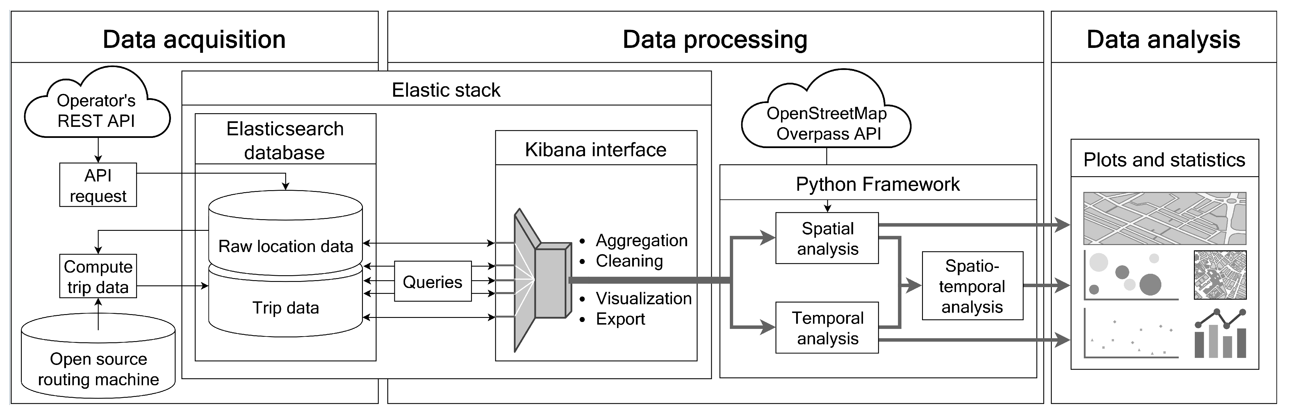
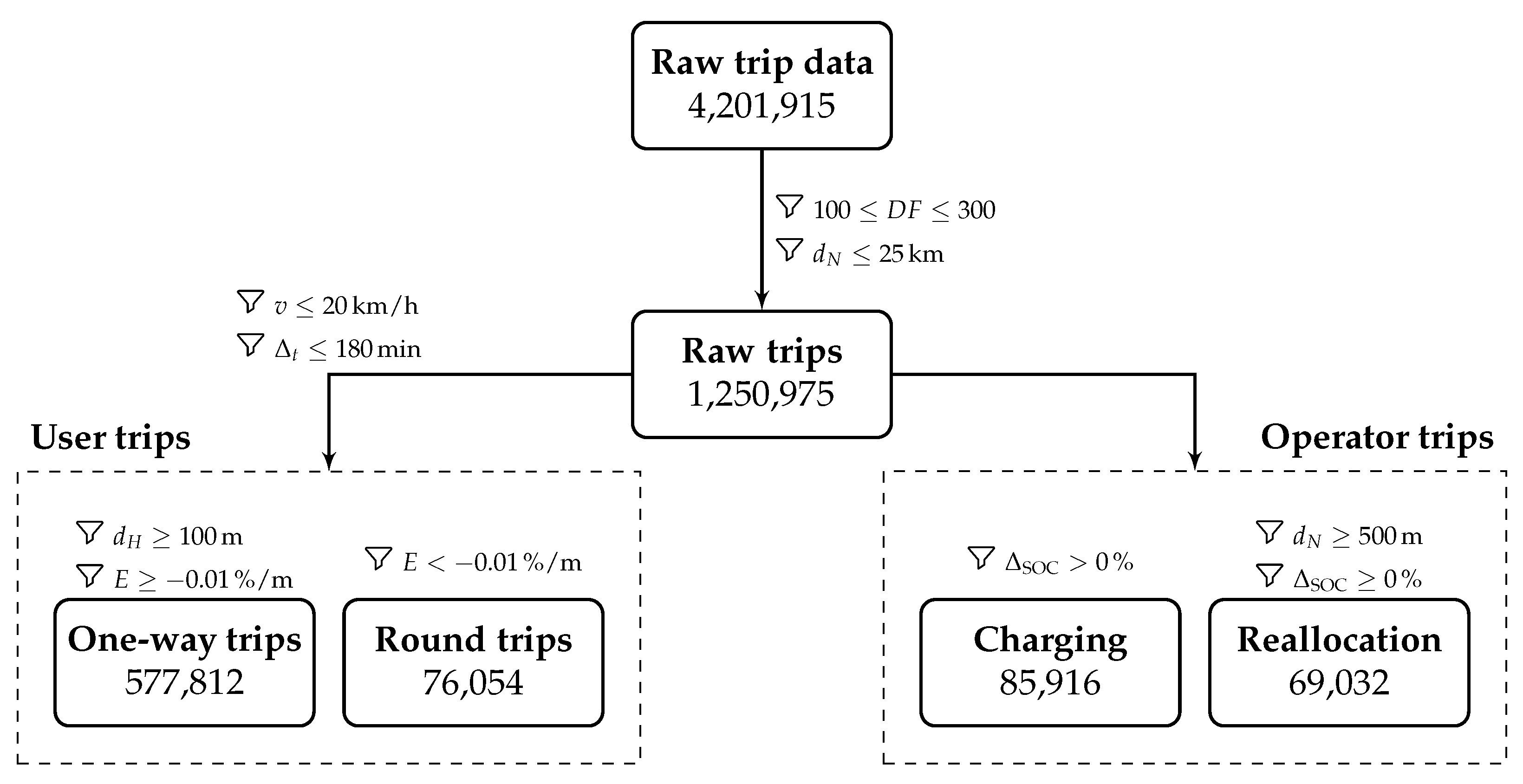
3. Data Set and Data Cleaning

In this section, all required steps related to data acquisition and processing are explained in detail to provide a transparent foundation for the spatiotemporal analyses. Our data pipeline in Figure 1 represents the concatenation of these steps towards the analyses. For the acquisition of our raw data set, the locations of the operator’s e-scooters are requested via an application programming interface (API) connection. It represents all available e-scooters at the time of the API query within a given zone. In our study, Berlin is the zone that is defined in the query by entering the respective zone ID. The returned data is structured as follows: each response contains information about the location of the e-scooters in world geodetic system (WGS84) coordinate latitude and longitude, with units in degrees expressed as decimal numbers and a 12-digit geohash format. Additionally, each e-scooter has a unique ID, the name of the operating zone, the e-scooter manufacturer, maximum velocity, battery state of charge (SOC) in percent, and the license plate number. These data are enriched by a timestamp with each query.
When an e-scooter is in use, it is not available in the record at that time. The last known location is linked to the location when the e-scooter reappears in the data set to create trip data. This origin and destination pair creates a trip, regardless of the trip duration ( Δ t ). The trip duration is derived from the last timestamp before and the first timestamp after a trip. The raw trip data is extended by the great-circle distance ( d H ), the network distance ( d N ), a detour factor ( D F ), the change in battery SOC ( Δ SOC ), and the energy consumption rate (E). We calculated d H using the haversine distance equation following Sinnott [61] implemented with the Python package haversine. We chose haversine estimation because of the more realistic assumption of a sphere, versus the assumption of a flat surface in the case of euclidean estimation. The resulting distance is given in meters. To determine d N , we used a local implementation of the Open Source Routing Machine (OSRM) [62]. The OSRM generates the trip distance for each trip based on the shortest bicycle route between origin and destination (see Figure 1). The underlying network is OpenStreetMap data. The OSRM routing is based on a further developed variant of Dijkstra’s shortest path first algorithm, using contraction hierarchies ([63,64]). From haversine and network distance, we derive D F = d N d H · 100 [65]. The e-scooters’ energy consumption rate E is the ratio of the change in SOC and the network distance, resulting in E = Δ SOC d N .
We queried the operator’s API from May 2019 to January 2020 and chose a temporal resolution of five minutes. The resolution is sufficient for our spatiotemporal analyses but not for precise trip velocity calculation. To enrich our data set with accurate velocities, we queried the API with a one-minute frequency over a four-week period and use this in our analysis to determine users’ trip velocities. Therefore, we merged the trips from the five-minute data set with the corresponding trips from the one-minute data set using the trip ID and enriched them with the velocities of the respective trips. However, due to the high data volume, the one-minute queries were not conducted over the entire period.
The data processing is embedded in an Elastic Stack architecture consisting of an Elasticsearch database, Logstash data processing and a Kibana web interface, which enables database queries. This framework has been used in previous research on big data processing (e.g., [66]). It provides multifaceted functionalities for data aggregation, cleaning, visualization, and export [67]. The processed data forms the basis for advanced investigations and can be extended by additional inputs like GIS-data for spatial analyses.
To present our filtering transparent and comprehensible, we first summarized the data cleaning parameters used in related spatiotemporal studies in Table 2. The temporal resolution of raw data in these related studies differs between 0.5 min and 30 min ; the most extended acquisition period amounts to 11 months [6]. Overall, traveled distance, duration, and average speed filters are the most common parameters for identifying user trips and separating them from outliers, reallocating, and charging trips. Nevertheless, there is no consistent pattern through the broad filters’ parameter range. In several studies, the filters’ parameterization is justified with reallocation or charging without explicitly labeling and clearly distinguishing them from outliers. Solely McKenzie [8], McKenzie [15] identifies charging and reallocation trips by average speed and trip duration and includes them in the analysis, but without differentiating between these two.
Based on the aggregated overview in Table 2, we verified our filter with a more comprehensive set of parameters (e.g., E, Δ SOC , d N , d H ). None of the presented studies uses the SOC change and the resulting energy consumption E per trip for classification. However, this approach offers advantages by enabling a more precise distinction between charging, reallocation, and round trips. Furthermore, it allows for identifying round trips using each trip’s energy consumption and comparing it with the average energy consumption of the one-way user trips. By filtering trips solely by distance, corresponding round trips could be excluded.
Subsequently, we elaborate on the selected parameters for data cleaning to present our data processing transparently. First, we filter outliers, e.g., false starts, traveled distance and trip duration anomalies, unauthorized location adjustment, and GPS tracking errors. Second, we label one-way trips, charging trips, reallocation trips, and round trips. Following Figure 2, we filtered out all trips with a network distance greater than 25 km and a detour factor outside the common range between 100 and 300 as outliers. By labeling our trips, we distinguish between operator and user trips. A user trip is defined by an average velocity of v 20   k m / h and a total trip duration of Δ t 180   min . We chose the velocity threshold of 20   k m / h assured by law for e-scooters in Germany. For the identification of one-way trips, we also excluded trips with a haversine distance below 100   m and an atypically high energy consumption rate of E 0.01 % / m . A haversine distance filter accounts for GPS errors and inaccuracies as the network distance is insufficient for filtering these. Obtained short distances in the haversine distance can result in significantly higher network distances, which could be missed by the defined threshold. We use the energy consumption rate threshold to distinguish one-way trips from round trips. In general, we assume that effects on the energy consumption rate roughly balance out on average for all trips. Possible factors that could affect the rate include topographic effects such as an uphill or downhill trip, increasing or decreasing the rate accordingly. It is also likely that the rate depends on the load of the e-scooter and thus the weight of the rider(s). In addition, increased energy consumption can be caused by uncommon detours between the start and endpoints. The resulting average of the energy consumption rate is E avg = 0.004 % / m , or a relative range of 250 m/%, respectively. This is the mean of the stated ranges in the operator’s app (20 km) and the one stated for end-user sales of the e-scooters (30 km). Therefore, we use E avg as a reference. In our case, a significant above-average energy consumption rate means that it is unlikely to be caused by one of the factors above. Since we could not find a reference value in the literature, we apply a factor of 2.5 times the average energy consumption E to identify round trips. Therefore, round trips are characterized by an average energy consumption rate of E < 0.01 % / m . Due to spatial proximity between origin and destination, the round trips’ average distance is short. However, in reality, longer distances (derived from Δ SOC and E avg ) were covered on these trips than the observed network distance suggests. Unlike one-way trips, we did not apply a minimum distance filter to round trips because the energy consumption rate precludes distances being caused by a GPS error. Rather, the energy consumption rate guarantees that the e-scooter covered a distance. We decided to consider the round trips as a phenomenon of user behavior and separate them from the one-way trips, since they distort the network distances of the trips, and thus the speeds and energy consumption rates.
Since both one-way trips and round trips are conducted by users, we summarize them as user trips. Of all trips recorded, user trips account for a share of 85 % , while charging and reallocation trips account for the remaining 15 % . Of all user trips, round trips account for 6.24 % . According to our data analysis, the average Δ SOC is about 7 % for one-way user trips and 12 % for round trips. The average trip duration matches these SOC changes. The duration of one-way trips is on average 7 min and 17 min for round trips. The average trip distance of one-way trips is about 1800 m . In contrast, round trips have an average network distance of only 500 m . Lastly, we obtain an average detour factor for user trips of 132. The authors Cubukcu and Taha [65] determined a slightly higher mean detour factor of 143 for Berlin. This deviation can be explained by the considered distances in their study, which are significantly longer and therefore cause a higher average detour factor for Berlin.
We separate charging and reallocation trips from user trips. These trips are performed by the operator and distort the analysis of user trips in terms of trip number, distance, change in SOC, and speed. If the SOC has increased during the trip, we label these as charging trips. A time limit for identifying charging trips is unsuitable because the operator can replace the discharged battery on the spot. Since e-scooters, based on our data, have an average relative range of 250 m /%, all trips with a trip distance d N of more than 500 m but without a decrease in the SOC are labeled as reallocation trips. For some reallocations, a charging process is performed at the same time.

4. Spatiotemporal E-Scooter Usage Patterns in Berlin

The recurring collection of e-scooter data by our system architecture gives an area-wide picture of trips in the considered business area of Berlin. On this basis, we conduct spatiotemporal analyses to provide a more detailed understanding of users’ mobility behavior. Figure 3 presents the spatial density of e-scooter trip destinations in Berlin over the nine-month observation period.
Besides e-scooter trip destinations, the operator’s business area boundaries (red line) and the operator’s warehouse locations (black triangles) are highlighted. It shows widely distributed trip destinations throughout the city with multiple hotspots indicating highly frequented locations. Sample hotspots are around Berlin Mitte, Tiergarten, Prenzlauer Berg, Friedrichshain, Kreuzberg and Moabit. Comparing the distribution of hotspots in Berlin to Austin or Minneapolis (e.g., [4,13]), Berlin shows a poly-centric pattern rather than a mono-centric one. This is consistent with previous studies that attribute Berlin’s poly-centric character to the diversity of land uses in urban neighborhoods and to the number of major transportation hubs with multi-modal services (e.g., [68,69]). Despite prohibited zones, the map indicates a significant proportion of rides that end in these areas. The density of ended e-scooter trips in the observation period is 1354 trips per km2 within the prohibited areas. In the permitted business area, the density is 4648 trips per km2. The volume of trips ending within the prohibited zones is only about 30% of the volume of trips that end inside of the remaining permitted business area. Therefore, it can be assumed that geofences have a significant impact on the trips at these areas.

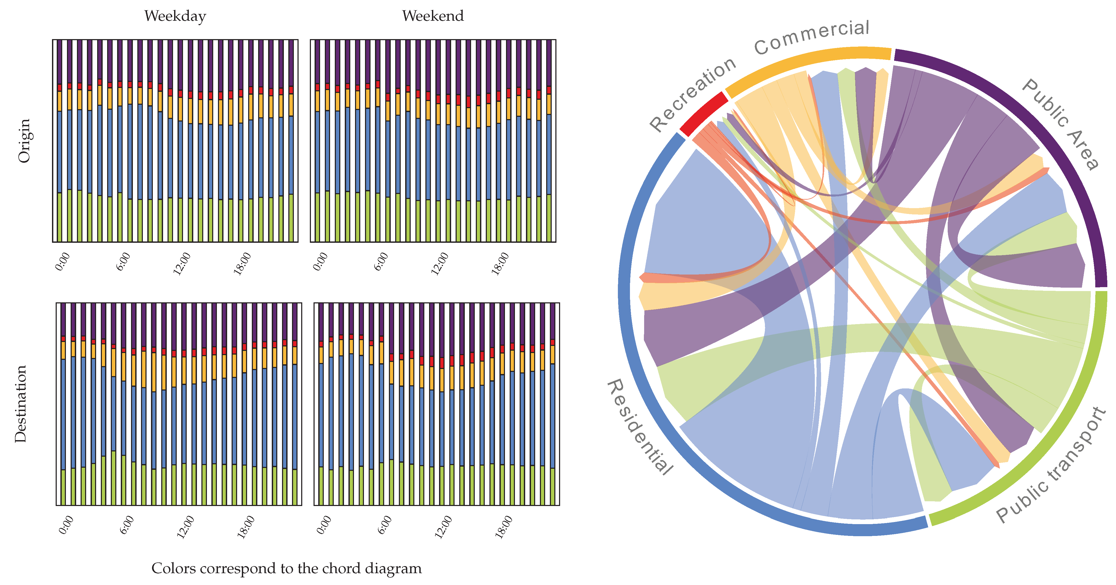
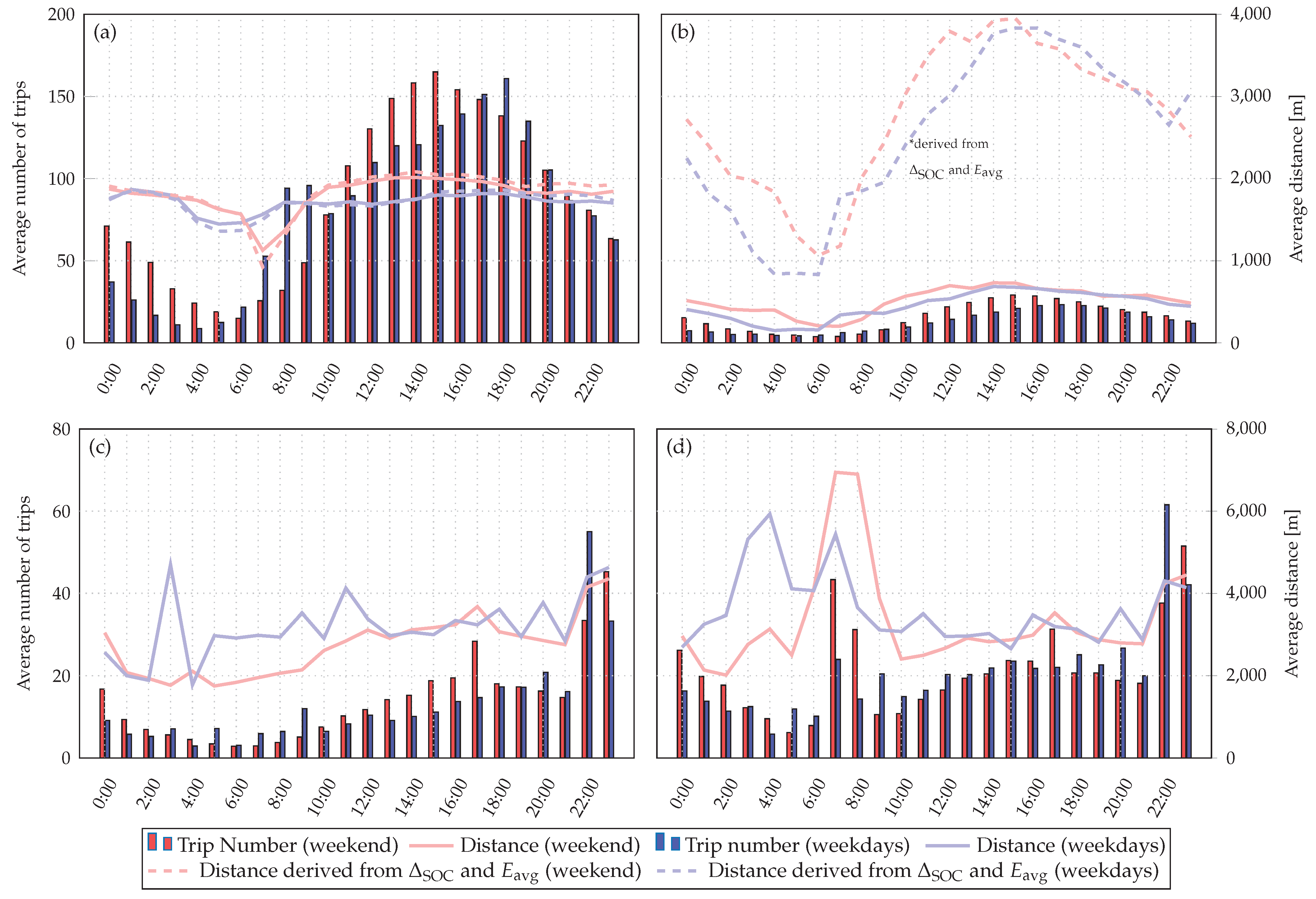
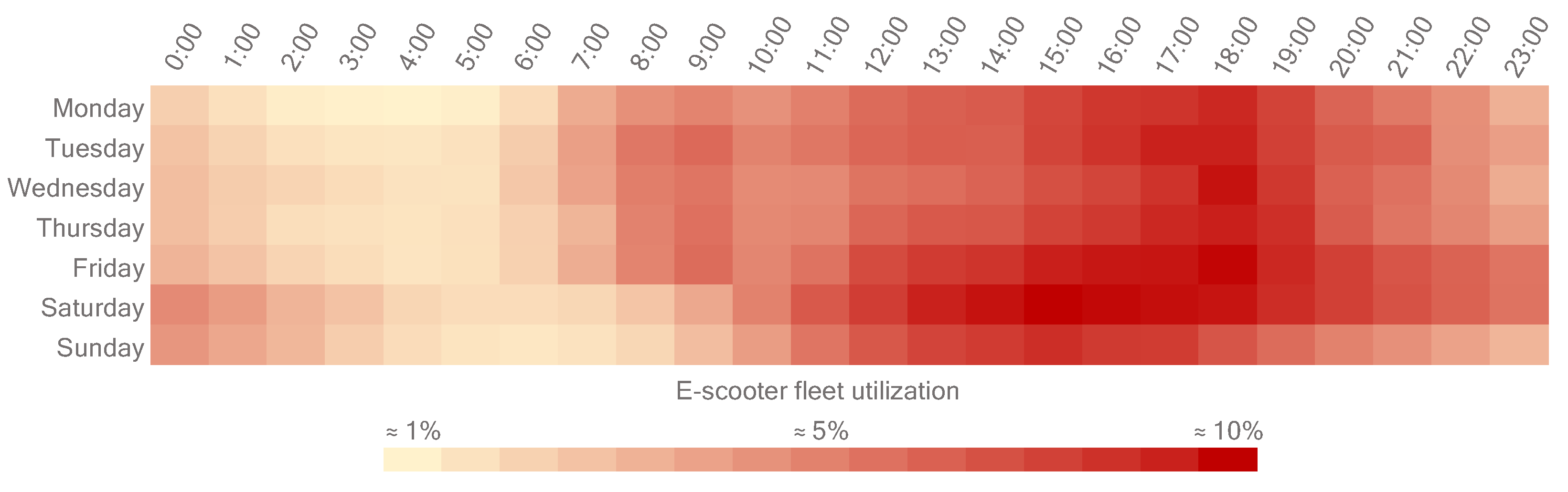
4.1. Temporal Analyses

The next step of our analyses encompasses the investigation of temporal usage patterns. Applying our criteria from Section 3, we labeled non-user trips as charging and reallocation by the operator. User trips were assigned to either one-way or round trips. Figure 4a–d summarizes the temporal patterns of one-way, round, charging, and reallocation trips divided into weekdays and weekends. In addition to the network distance, we have plotted a distance derived from Δ SOC and E avg (cf. Section 3). While our network distance for one-way trips in Figure 4a is strongly related to the calculated distance, it shows significant disproportion for the round trips in Figure 4b. In general, the four trip types show different daily characteristics depending on weekdays and weekends in terms of the average number of trips and distance. Most of the one-way and round trips occur on weekend afternoons, and at about 6 p.m. on weekdays. During the weekend peak, the trips with the longest average distance of about 2000 m were completed. Apart from this, the average distance of one-way trips remains at a relatively constant level of about 1800 m . The most significant deviation occurs on weekends between 6 a.m. and 8 a.m., with average distances around 1200 m . In contrast, the distances at this time on weekdays have a local maximum, with average distances of about 1700 m . It is noteworthy that the round trips, apart from overall significantly higher distances derived from Δ SOC and E avg , also have a considerably larger peak-to-peak amplitude in the course of the distances of about 800 m to 4000 m .
The numbers of one-way trips on weekends from midnight to 5 a.m. are significantly higher than during that time on weekdays. These trips might be related to the city’s nightlife and indicate an entertainment purpose. There is also a local peak in the average trip distances between 1 a.m. and 3 a.m. on weekdays. The reduced public transport operation in Berlin from Monday to Friday between 1 a.m. and 4 a.m. might explain this course. Additionally, Figure 4a shows a significant increase in one-way trips on weekdays at commuting times from 7 a.m. to 9 a.m and 5 p.m. to 7 p.m. These local peaks might indicate proportionate commuting traffic. In addition, one-way trips on weekends do not show the typical pattern of two local peaks at commuting times.
While presented divergence of one-way and round trips in Figure 4a,b points to the problem of recording round trips together with one-way trips, the plot thus also confirms the rationality of labeling these. Due to the mentioned aspects in Section 3, the observed round trips’ average network distance is short. According to the trips’ energy consumption, significantly longer distances were covered on these trips than on one-way trips. Examples of round trip intentions can be pick-up trips, sightseeing, or testing the new mobility concept, whereas commuting is not reasonable for round trips. Further, the peaks at commuting times for one-way trips do not occur for round trips, which supports our assumption that the peaks in Figure 4a are due to commuting, since the remaining pattern is similar to one-way trips.
Compared to other studies, the temporal pattern of daily e-scooter trips in Indianapolis by Mathew et al. [18] shows a similar course as Figure 4a. Temporal patterns for all days of the week by McKenzie [15] also display a similar trend, but the demand peaks are closer to midday. The global peak of e-scooter rides in Washington D.C occurs in the early afternoon on the weekend. This result is in line with our analysis for Berlin. Noland [17] measured the most trips on weekends for Louisville. However, no differentiation was made between weekdays and weekends, which reduces the comparability. The temporal patterns of Younes et al. [16] and Zou et al. [9] are consistent with data analyses of the previous studies.
Figure 4c,d visualize the characteristics of charging and reallocation trips by the e-scooter operator. Due to high e-scooter utilization during the day, charging trips peak at 10 p.m. This trend occurs on both weekdays and weekends. The reallocation trips also peak in the early morning from 7 a.m. to 9 a.m. The e-scooters’ range (roughly 25   k m ) with average trip distances of about 1800   m allows for numerous trips before the e-scooters need to be recharged. This daily recharging routine is carried out mainly in bundles of e-scooters in the late evening combined with their reallocation. E-scooter traffic leaves high demand locations underrepresented after the morning and afternoon peak hours, requiring two time slots per day to reallocate scooters. The magnitude of average charging and reallocation trip distances is volatile as the users’ behavior and e-scooter drop-off locations are difficult for the operator to predict. Within the study of Agora Verkehrswende [70] which was conducted in cooperation with the German association of cities and the German association of towns and municipalities, the authors call on operators to shift to emission-free electric vehicles for the maintenance and redistribution of e-scooters in the future. To reduce the need for e-scooter redistribution, an alternative solution might be dynamic pricing models. These create monetary incentives for riders to take scooters in areas of lower demand and thereby enable a more efficient response to trip demand and a higher fleet utilization rate.
To further examine the fleet utilization of the e-scooter operator, we illustrate temporal hotspots of the fleet usage in Figure 5. However, the temporal course follows a similar pattern to the user trips in Figure 4. During weekdays, there are fewer night-time trips and two local peaks throughout the day. From 6 a.m. to 9 a.m., there is a local peak from Monday to Friday. The second peak occurs between 4 p.m. and 7 p.m. On weekends, especially on Friday evenings and Saturdays with an upcoming free day (most businesses are closed on Saturday and Sunday in Germany; most retail stores are also closed on Sunday in Germany), the number of trips slightly increases throughout the day until around 3 p.m. It then slightly decreases hourly until 2 a.m., to a minimum of about 1 % . Remarkably, the maximum share of e-scooter fleet utilization per hour accounts only for 10 % .
A maximum fleet usage rate of 10% by Berlin’s largest provider means that approximately 300 e-scooters are on the road at peak times. The daily average of e-scooter trips is approximately 2300 for the respective operator. Even if the daily trips of all five Berlin providers are aggregated at the same usage rate, the generated trip volume is small compared to pedestrian, bicycle, and car traffic in Berlin. A representative survey about residents’ mobility behavior shows that a Berlin resident takes an average of 3.5 trips per day. With a population of about 3.6 million, this corresponds to a daily average of about 12.6 million trips in total excluding tourists [71]. In 2017, 30% of trips in Berlin were made on foot, 27% by public transport, 25% by motorized private transport, and 18% by bicycle [72].

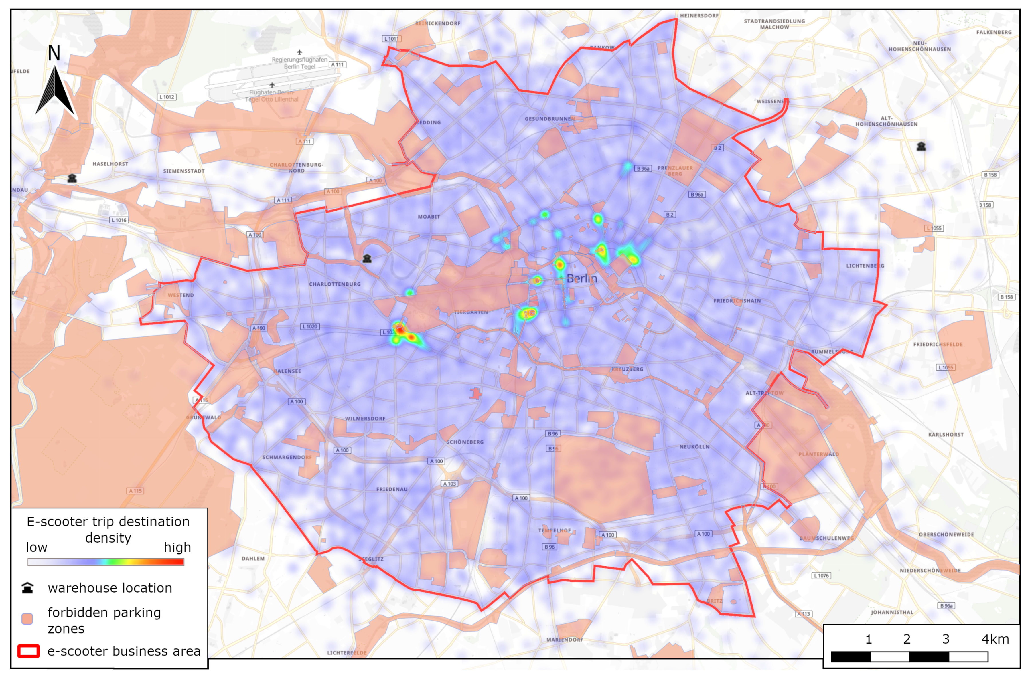
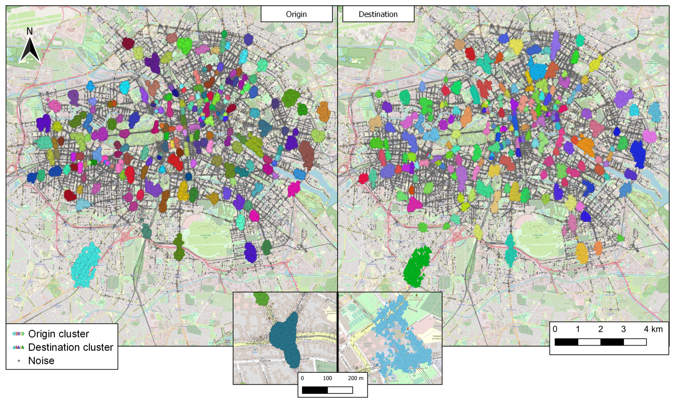
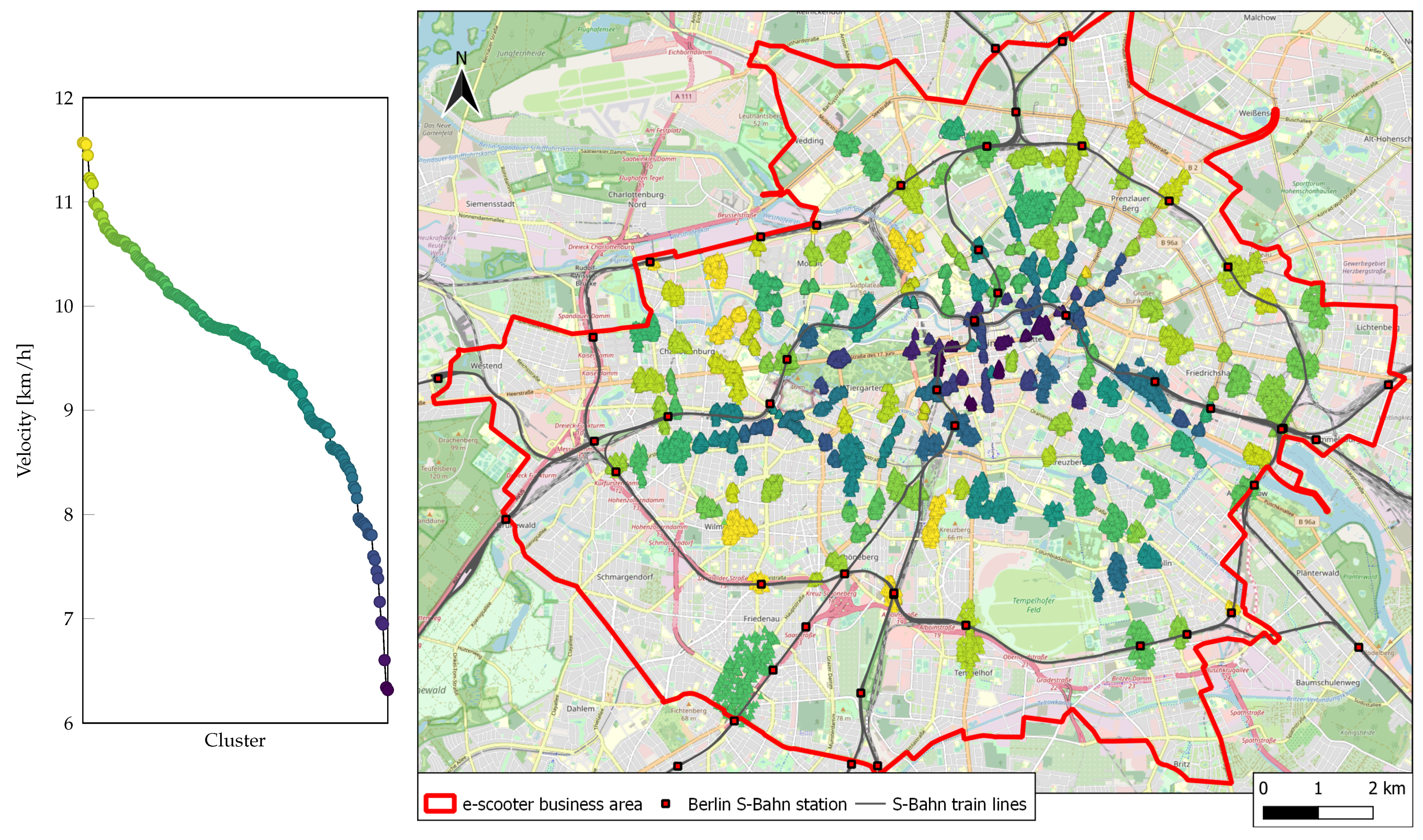
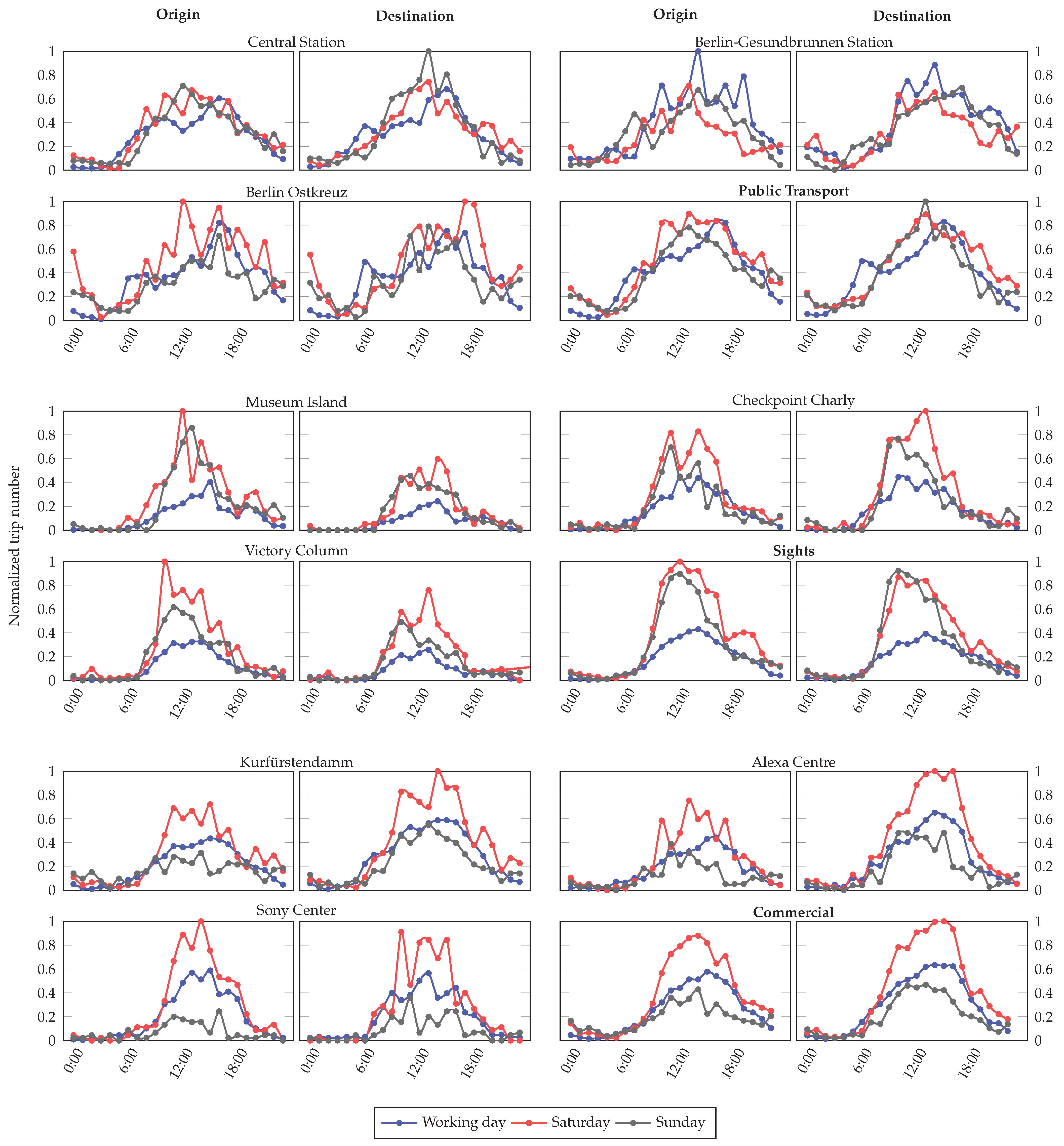
4.2. Spatiotemporal Analyses

To conduct spatiotemporal analyses, we split the trip data based on land use of origin and destination. Thereby, we can spatially aggregate information about possible activities and users’ trip intentions. First, we gathered available OpenStreetMap (OSM) land use data of five different area types using OSM Overpass API: Residential, Commercial, Recreation, Public, and Public transport. More specifically, we query the OSM database for data tagged with the attributes landuse = { residential , commercial , recreation } , and public transport = platform . All remaining areas were considered as public areas. Typical building types, spaces, the corresponding areas’ spatial sizes, and trip shares are listed in Table 3. Then, we checked the trips’ origins and destinations for intersections with the defined area types. Trips starting or ending in mixed area types have been omitted from the analysis, as they account for only about 2% of all trip data. We subdivided the trip distribution by land use into an aggregated hourly bar plot for weekdays and weekends regarding origin and destination on the left in Figure 6. In our land use analysis, shared e-scooter trip origins and destinations can be assigned to areas that are dominated by a certain usage. Departures or arrivals in these areas are not necessarily associated with this use. Nevertheless, causality can be assumed due to the large data point number in our analysis (e.g., [8,13,15,18]).
It is remarkable that around 8 a.m. on weekdays, there is an increase in destinations in public transport areas. Simultaneously, the share of residential origins rises slightly. This relationship could suggest that e-scooters function as part of commuter trips and improve public transport connectivity. In contrast, public transport origins remain at a constant level during weekdays and weekends. Furthermore, destinations in residential areas increase steadily on weekdays starting in the afternoon. This development could result, among other activities, from the return trips of commuters. In general, destinations in commercial sites grow during the morning and peak at noon on weekdays. This could indicate for occasional purchases and work paths made with e-scooters. Regarding destinations in public areas on weekends, there is a considerable increase during the morning, and this trend builds to a high plateau during the afternoon. Additionally, the origins in public areas take a similar pattern to the destinations. According to our spatial categories classification, recreational areas take up only a small share of all trips on both weekdays and weekends. Nevertheless, a higher proportion of trips to and from these areas is observed on weekends.
However, the bar plot does not represent the trip number between the considered land use types. To visualize the relationship between these land use types, we created a chord diagram, shown on the right side of Figure 6. The arrows represent the trips between different land use types. The width of the arrows indicates how many trips have occurred. Each arrow’s color corresponds to the origins’ land use type. The partitioning of the outer ring represents the number of trips that start and end in the respective area. Compared to Table 3, the partitions of the outer circle do not correspond to the actual area sizes. With only a share of 2.2 % of total area, the proportion of about 20 % of all trips directed to the public transport network and 22 % that start there is relatively large. The largest share of trips with 39 % starts in residential areas. Also, 43 % of the trips end in residential areas, accounting for the largest share of trip destinations. Despite its largest share in terms of space ( 38 % ), public areas account for only 24 % of trip origins and 21 % of trip destinations. Moreover, it is remarkable that the highest difference between incoming and outgoing trips occurs with 4 % in residential areas.
After using the temporal bar plot and the chord diagram to couple temporal patterns with spatial trip patterns, we want to extend the spatial analysis to a more granular level. As mentioned in Section 2, spatially fine-resolved clusters of origin and destination can be used to identify highly frequented routes between hotspots. It can also facilitate identifying bottlenecks and underrepresented areas in the public transport network or determine the need to expand transport routes. Highly frequented clusters can indicate the necessity of connections to be improved to the public transport network. Furthermore, abnormally low average speeds between clusters can serve as an indicator of congested traffic routes. It can also facilitate an understanding of location-specific or POI-related temporal usage patterns.
As presented in Section 2, a typical procedure for clustering is the segmentation of a considered area into uniform quadrants. However, this approach neglects the actual arrangement and density of the objects, and the built environment. Spatially asymmetrical arrangements in the urban built environment are common in most European cities. Due to its basic suitability for non-linearly separable clusters, density-based algorithms such as DBSCAN, or OPTICS are appropriate for these urban contexts and also generally intended for geodata (e.g., [73,74]). Since we assume an unknown number of origin and destination clusters and an uncertain degree of distribution of trips due to arbitrary ones, DBSCAN can be superior to commonly used algorithms, e.g., the K-Means algorithm, for our extended spatial analysis (e.g., [73,75]). DBSCAN can filter out insignificant noise and thereby enables focusing on core areas. Moreover, it is not necessary to predefine the cluster number. However, when using DBSCAN, the optimal combination of minimum points inside a cluster and maximum distance parameters is not an intuitive task to reach optimal cluster stability.
An advanced method to DBSCAN is the utilization of HDBSCAN as a hierarchical cluster algorithm. It addresses the problem of detecting meaningful clusters in varying density data [76]. Therefore, a hierarchical cluster algorithm aims to achieve the finest possible resolution of the clusters without having too many of them break down into smaller clusters. This difficulty arises locally, especially in very heterogeneous arrangements due to the built environment and individual user behavior. For example, it is necessary to identify clusters in wider built environments, as well as in the case of narrow and very dense arrangements. On the one hand, a large junction can cause high distances between the e-scooters on the sidewalks, which can nevertheless be assigned to a specific location. On the other hand, very dense arrangements in more frequented urban areas can occur because of multiple POIs. To tackle this, we use HDBSCAN to maximize the overall stability of the composed clusters by optimizing all possible DBSCAN solutions given a value of minimum points inside a cluster. This results in hierarchical clustering, instead of a ’flat’ one as in the case of DBSCAN. HDBSCAN thereby enables us to identify clusters in different types of urban structures by individual density levels. Since HDBSCAN optimizes the density level of the clusters globally to achieve a stable cluster arrangement, only one parameter is necessary for the cluster analysis. As an input parameter for HDBSCAN, we need to define a necessary daily average of trips over the observation period to form a cluster. We defined a threshold of an average of two trips that need to start or end at a location per day and assume an average below this threshold to be noise. Therefore, the minimum number of points necessary to form a cluster is 546, which corresponds to our observation period of 273 days. This means that at least a number of 546 scooter departures, or arrivals (or 2 per day for the 273 day observation period) must be concentrated at a location to form a cluster. The density within which the 546 e-scooters must be located is optimized by HDBSCAN [76]. This assumption can be interpreted in such a way that we suppose that on average one departure, or arrival per day may be coincidental. From an average number of two arrivals or departures per day, we assume a pattern.
Figure 7 visualizes the computed clusters and surrounding noise (gray dots). The analysis of 577,812 one-way user trips resulted in 206 trip origin clusters (circles) and 194 trip destination clusters (triangles). Varying colors are used to distinguish the clusters. 46.4 % of all trips start within the origin clusters, and the rest are considered as noise. Regarding destinations, 44.6 % of all trips end within a cluster, the rest are classified as noise. 22.2 % of all trips are inter-cluster routes, starting and ending within clusters. Using HDBSCAN results in a dispersed arrangement of clusters throughout Berlin. Most clusters are sufficiently granular to assign them directly to a POI as the clusters match the city’s built environment, and in several cases, take on the asymmetric shape of the corresponding built environment (see zoomed clusters in Figure 7). Due to the sharing systems’ free-floating character, many trips start at locations where others previously ended. As a consequence, departure and arrival clusters largely coincide. Apart from this, origin- or destination-only clusters also exist. Since the corresponding e-scooter trips are insufficient to disperse these accumulations, the operator has to reallocate the e-scooters at these locations.
Figure 8 visualizes the average trip speeds per destination cluster. The left side shows the average trip velocities to the clusters and serves as a legend for the cluster visualization on the right. 55 % of all clusters indicate average trip velocities between 8 and 10   k m / h . About 10 % of the clusters have rather low average velocities of 6 to 8   k m / h , and 35 % have rather high average velocities of 10 to 11.5   k m / h . Similar to our analysis, the results of Almannaa et al. [12] indicate average e-scooter trip speeds between 8 to 10   k m / h for two temporal clusters of weekends and weekdays. However, as more location specific clusters are identified within our spatial analysis, we have found a wider range of average velocities from 6 to 11.6   k m / h . The average trip speed to a cluster can serve as an indicator for the clusters’ integration to the transport network or how frequented the corresponding routes to these clusters are.
In our analysis, velocity deviations cannot be caused by round trips, according to our definition. Since we included only one-way trips in the cluster analysis, significant detours are excluded from trip data. However, average trip velocities are calculated based on the shortest path between trip origin and destination and in reality, drivers do not necessarily take this optimal route. Drivers might stop temporarily within a trip or vary from the shortest path, causing our analysis to be biased towards lower average speeds. Still, the calculated velocities are significantly lower at central highly-frequented clusters than at clusters off these areas. In central areas of high (pedestrian) traffic, such as Alexanderplatz, Brandenburg Gate, or Unter den Linden, the calculated average speeds are at about 6   k m / h . Compared to the e-scooters’ potential in clusters with average speeds of about 11   k m / h , the use in congested areas can be questioned. Here, urban planning should conduct measures to weigh-up benefits of e-scooter usage against its associated problems, such as parking violations, congested bike lanes, and potential accidents with pedestrians (e.g., [47,48]). The introduction of geofences for no-parking and low-speed zones is a short-term way to regulate e-scooter use [40]. Our results show that geofences could significantly reduce e-scooter usage in these areas. Nevertheless, we see noticeable trip volume in corresponding prohibited zones (see Figure 3). Lusk et al. [77] and Marqués and Hernández-Herrador [78] show that a segregated bicycle network increases the trip number and further reduces the number of bicycle-related accidents on these routes. By adapting these findings to e-scooter usage, separating bicycle and e-scooter network from motorized traffic could reduce detours, increase average speeds, and mitigate conflict situations with other traffic participants. Overall, this separation could lead to increased attractiveness and e-scooter user numbers. The spatial allocation of traffic and parking space is currently being discussed in the course of emerging micro-mobility concepts. Some studies criticize that the spatial allocation deviates considerably from the modal split (e.g., [37,70,79]). Although bicycle trips accounted for 15 % of total trips, cyclists were only allocated a 3 % share of traffic space in Berlin in 2014. In contrast, motor vehicles were allocated a share of 39 % [80]. Following Gössling [41], Laa and Leth [37], and Nello-Deakin [79], we endorse that urban planning should address this disproportion. These authors suggest providing more space for micro-mobility infrastructure. This should include developing both designated parking areas and a street network for micro-mobility. In areas of shared use with motorized traffic, consideration should be given to limiting speed levels towards bicyclists’ and e-scooters’ maximum speeds. Our cluster analysis identifies areas with high e-scooter trip frequency and allowed for differentiation based on temporal patterns and average velocities. It could guide the implementation of appropriate location-specific measures and can be utilized for their prioritization.
Regarding public transport, the algorithm forms clusters at almost all stations of the Berlin S-Bahn line Ringbahn, a ring-shaped local train line on the city’s outskirts (see Figure 8). Clusters located at these stations suggest a direct connection between the trips and the public transport connections, as some stations are isolated from other activities and areas (e.g., S Jungfernheide, S Beusselstraße, S Westhafen, Berlin Südkreuz). Most clusters at stations of the Ringbahn have an above-average speed. Additionally, some clusters at more central transportation nodes have high above-average speeds, such as the north exit of Berlin Hauptbahnhof with about 11   k m / h . This observation suggests that these locations are well-connected to the road and bicycle network or that corresponding routes have a comparatively low traffic load. Deepening the understanding of clusters and their characteristics, we depicted several clusters and categorized them based on the type of nearest POI into sight-, public transport-, and commercial-related clusters. Sights are popular landmarks and tourist attractions, while public transport nodes are main train stations and Berlin S-Bahn stations. Commercial-related places are shopping malls or shopping miles. Thereby, we can foster our statements about e-scooter usage at these locations and make reasonable suggestions about users’ travel behavior. We visually examined the individual cluster categories for similarity in temporal usage patterns in Figure 9. With this, we found similar temporal patterns within the categories. We depicted the day’s temporal course of an average weekday, Saturday, and Sunday. In addition to three specific examples per category, we have supplemented a cumulative plot that includes five POIs per category. For this plot, the three shown examples and two additional clusters from the corresponding category were summarized to smooth out individual outliers and distinctly highlight each category’s characteristics.
Overall, there are differences in the temporal pattern within the categories depending on the week’s day. Weekdays show clear peaks of trips that start or end at public transport stations at typical commuting times. These peaks are not observed on weekends. It further supports the hypothesis that e-scooters are used for intermodal commuting trips at these times. In addition, these peaks are not seen in the Sights and Commercial POI categories. Further, trip frequency to and from the public transport stations considered is quite evenly distributed across all days of the week. At sights, trip frequency takes a bell curve on all days of the week with the maximum during midday. In contrast to an average weekday, significantly more trips are registered on Saturdays and Sundays. For the commercial areas, the overall trend is similar to the sights. However, the peak shifts slightly to the afternoon. Additionally, there is a significant difference on weekends. Due to the usual day of rest on Sundays in Germany, the frequency of trips is significantly lower than on weekdays and is exceptionally lower than on Saturdays, when most trips occur.
We performed a cosine similarity analysis for all combinations of our selected clusters to test our cluster categories’ similarity using a statistical measure that reflects two non-zero vectors’ similarity. The metric measures the cosine angle of two inner product vectors, generating a similarity measure for each pair of temporal activity signatures. The resulting measure yields numerical values between 0 (most dissimilar) and 1 (most similar) for each of our cluster pairs, given only positive time series values. To create a vector for each cluster, we concatenated the time series values of origins and destinations for all average weekday, Saturday, and Sunday (see Figure 9). The cosine similarity values are shown in Table 4.
All clusters, apart from Checkpoint Charly and Kurfürstendamm, have the highest cosine similarity values with clusters of their corresponding category. Thereby, they reach almost consistently a similarity value above 0.90 within the categories. This result indicates that the categories can be sufficiently distinguished from each other, with the public transport category achieving the highest similarity values. However, the cluster Checkpoint Charly has a slightly higher correspondence with Kurfürstendamm than with Museum Island, measured by cosine similarity values. In addition, Kurfürstendamm has a higher similarity with the Gesundbrunnen cluster than with the Potsdammer Platz cluster from its assigned category. The slight deviations from the assigned category may be explained by assigning our clusters to the nearest POI. Nevertheless, a distinct assignment is not feasible for all POIs because of mixed-use at specific locations. Besides many retail stores at the Kurfürstendamm, it is a place where many people go to their workplaces and use one of the subway stations to commute to work. The mixed-use could explain the tendency to the higher similarity of Kurfürstendamm to the public transport category. Furthermore, Checkpoint Charly is located in the middle of a shopping mile, which could explain the high similarity to Kurfürstendamm. In summary, cosine similarity analysis could complement visual classifications to distinguish POIs more precisely.

5. Limitations

Related to biases mentioned by McKenzie [15], our study does not provide information about the e-scooter ridership demographics in Berlin. Although Figure 3 indicates widespread coverage in Berlin, it is challenging to draw clear conclusions about which strata of the population primarily uses e-scooters. Thus, transport equity questions were not addressed in this study.
The investigated data set is largely based on a five-minute temporal resolution, which reveals weaknesses, especially for trips of short distances that have a duration of less than five minutes. First, the duration of such trips cannot be clearly determined. Second, no reliable conclusions can be made about the average speed. To mitigate this shortcoming, we analyzed a one-minute data set over one month for the average velocities (cf. Section 3).
Regarding spatial analysis of land use types, we selected five different land use types from OSM. In certain areas, these types overlap which results in an assignment of areas to multiple land uses. As mentioned in Section 4.2, we omitted trips that originated or arrived in areas of multiple land use types. Although these non-analyzed trips account for only 2 % of all trips, they still represent a limitation of our land use analysis.
Through our investigations, we infer travel intentions from temporal, spatial, and mixed patterns in mobility data, and while some conclusions may seem intuitive, none of these should be taken as evident. Further studies are indispensable in examining and substantiating extensive data analyses with qualitative methods such as user surveys.
Despite the advantages of spatial clustering, some clusters could not be assigned to a single POI. In these cases, the results can be biased by multiple activities, impeding the identification of distinct patterns, as the activities can not sufficiently be segregated from each other. A resulting implication for future research to address this issue is to incorporate the temporal dimension in the process of clustering. This should include a three-dimensional input for the clustering algorithm with the trips’ start or end times. For instance, at a large public transport station with shopping facilities, spatiotemporal clusters could foster the distinction between the shopping and transportation activities of e-scooter riders.
The results of the HDBSCAN are sensitive to the input parameters for the cluster formation. We argue that the definition of these parameters is application-specific and that we selected an appropriate threshold for our investigations. Nevertheless, we cannot guarantee that it is the most efficient selection. The focus of the clustering was to generate POI-specific results that required the exclusion of noise. In this way, the proportion of trips that we could not directly assign to a specific POI is substantial at about 55 % . As these excluded trips also describe the e-scooter user behavior, a prioritization shift in the clustering in further research might need to be reconsidered.

6. Conclusions

Shared e-scooters have become widespread in US and European cities over the past three and a half years. E-scooter use has been investigated to date in mostly American cities based on provider data. In this study, we examined how e-scooters are used in space and time in Berlin (RQ1) and how cluster and land use type analyses can contribute to an improved understanding of e-scooter usage (RQ2).
In addition to removing outliers, the applied filters allow precise segregation between user, reallocation, and charging trips. This enabled a differentiated view of the temporal trip patterns. We identified round trips by filtering the energy consumption rate and approximated their distance. The fleet utilization rate is at a maximum of 10 % and is reached on Saturday afternoons. Our results indicate a wide coverage of the urban area of Berlin. In contrast to often mono-centric patterns, Berlin shows a poly-centric arrangement. E-scooters are also parked or activated for a ride in zones restricted by geofences. Still, considering our data from the largest operator in Berlin, we can highlight the efficacy of geofences. They reduce the e-scooter parking in prohibited zones by almost 70 % .
Using spatiotemporal analysis to address RQ2, we examined the trip numbers between five different land use types. With this, we identified commuter trips to public transport in the morning and afternoon on weekdays and increased ridership activity in public areas on weekends. By applying HDBSCAN, we discovered spatially more fine-resolved clusters compared to grid-based approaches. Based on 577,812 one-way trips, 206 origin and 194 destination clusters were identified. We analyzed the destination clusters for average velocities and used them to identify congested clusters and clusters that can be accessed more quickly. According to our results, average velocities in areas close to the city center are significantly lower than in the outskirts. We enhanced the analysis by categorizing specific POIs, highlight the temporal user patterns of public transport, commercial areas, and sights, and further underpin the derived statements by a cosine similarity analysis to complement and evaluate our classification. This demonstrates POI-specific e-scooter travel behavior and allows more specific conclusions about the use intention. These analyses of shared e-scooters in Berlin offer several indicators to improve the understanding of spatiotemporal usage. It could guide the implementation of appropriate location-specific measures and can be utilized for their prioritization. Based on our findings, we recommend location-specific analysis of usage patterns in practice and research, enabling more effective design of regulatory measures by authorities, as usage patterns at different POIs differ significantly. Further, a better understanding of POI-specific usage would allow operators to adapt fleet management more adequately to the demand. By directly categorizing usage patterns at specific POIs, operators can reduce the mass of unused e-scooters. A suitable method for POI assignment can be density-based clustering algorithms with noise. For filtering or labeling of e-scooter trips, we recommend the use of energy consumption filters if applicable. This leads to a more precise trip classification and allows the identification of round trips in the data. To support future research directions, we propose the following enhancements. Especially evidence from our study on the combined use of e-scooters in combination with public transport justifies the analysis of incentive effects of e-scooters on public transport. Research should emphasize the complementary function of e-scooters and the question of whether commuters are more likely to abstain from using a car as e-scooters cover the first or last mile in public transport. The observed differences in calculated average velocities across urban area suggest future research investigating related infrastructural conditions in the built environment. Thereby, structural dependencies that cause correlated congestion patterns of e-scooter usage in urban road networks can be revealed. Our results show a significant effect of geo-fenced restricted zones on e-scooter usage behavior. In addition, our results suggest a shared use of pedestrian and bicycle paths with e-scooters. In this context, we concur with the recommendations of some authors and encourage a reconsideration of traffic space allocation in light of the disproportionate spatial share relative to the modal split. Regarding the identified temporal patterns of e-scooter usage for different POI categories, a representative user survey can substantiate these data-driven inferences. Further, growing availability of data sources like traffic accident data (e.g., [81]) enables the integration of more extensive indicators to sharpen practical implications that can enhance safety in urban traffic.

Author Contributions

M.H.: conceptualization, writing—original draft, formal analysis, investigation, methodology, visualization, project administration. T.K.: visualization, investigation, writing—review & editing, methodology. T.B.: investigation, formal analysis, writing—original draft, writing—review & editing, methodology. L.T.: software, data curation, methodology. M.H.B.: writing—review & editing, supervision, conceptualization. All authors have read and agreed to the published version of the manuscript.

Funding

The publication of this article was funded by the Open Access Fund of Leibniz Universität Hannover.

Institutional Review Board Statement

Not applicable.

Informed Consent Statement

Not applicable.

Data Availability Statement

The data presented in this study are available on request from the corresponding author. The data are not publicly available due to privacy concerns.

Conflicts of Interest

The authors declare no conflict of interest.

References

  1. Lazarus, J.; Pourquier, J.C.; Feng, F.; Hammel, H.; Shaheen, S. Micromobility evolution and expansion: Understanding how docked and dockless bikesharing models complement and compete—A case study of San Francisco. J. Transp. Geogr. 2020, 84, 102620. [Google Scholar] [CrossRef]
  2. National Association of City Transportation Officials. Shared Micromobility in the U.S.: 2019. 2020. Available online: https://nacto.org/wp-content/uploads/2020/08/2020bikesharesnapshot.pdf (accessed on 14 September 2021).
  3. Schellong, D.; Sadek, P.; Schaetzberger, C.; Barrack, T. The Promise and Pitfalls of E-Scooter Sharing; Boston Consulting Group Publications: Europe, 2019; Available online: https://image-src.bcg.com/Images/BCG-The-Promise-and-Pitfalls-of-E-Scooter%20Sharing-May-2019_tcm96-220107.pdf (accessed on 14 September 2021).
  4. Bai, S.; Jiao, J. Dockless E-scooter usage patterns and urban built Environments: A comparison study of Austin, TX, and Minneapolis, MN. Travel Behav. Soc. 2020, 20, 264–272. [Google Scholar] [CrossRef]
  5. Mobility Foresights Transportation. Electric Scooter Sharing Market in US and Europe 2019–2025. 2020. Available online: https://mobilityforesights.com/product/global-micromobility-market/ (accessed on 14 September 2021).
  6. Jiao, J.; Bai, S. Understanding the Shared E-scooter Travels in Austin, TX. Int. J. Geo-Inf. 2020, 9, 1–12. [Google Scholar] [CrossRef] [Green Version]
  7. Noack, R. Electric scooters have arrived in Europe and a lot of people there hate them too. The Washington Post, 9 July 2019. [Google Scholar]
  8. McKenzie, G. Urban mobility in the sharing economy: A spatiotemporal comparison of shared mobility services. Comput. Environ. Urban Syst. 2020, 79, 101418. [Google Scholar] [CrossRef]
  9. Zou, Z.; Younes, H.; Erdoğan, S.; Wu, J. Exploratory Analysis of Real-Time E-Scooter Trip Data in Washington, D.C. Transp. Res. Rec. J. Transp. Res. Board 2020, 2674, 285–299. [Google Scholar] [CrossRef]
  10. Boglietti, S.; Barabino, B.; Maternini, G. Survey on e-Powered Micro Personal Mobility Vehicles: Exploring Current Issues towards Future Developments. Sustainability 2021, 13, 3692. [Google Scholar] [CrossRef]
  11. O’Hern, S.; Estgfaeller, N. A Scientometric Review of Powered Micromobility. Sustainability 2020, 12, 9505. [Google Scholar] [CrossRef]
  12. Almannaa, M.H.; Ashqar, H.I.; Elhenawy, M.; Masoud, M.; Rakotonirainy, A.; Rakha, H. A comparative analysis of e-scooter and e-bike usage patterns: Findings from the City of Austin, TX. Int. J. Sustain. Transp. 2020. [Google Scholar] [CrossRef]
  13. Caspi, O.; Smart, M.J.; Noland, R.B. Spatial associations of dockless shared e-scooter usage. Transp. Res. Part D Transp. Environ. 2020, 86, 102396. [Google Scholar] [CrossRef]
  14. Feng, C.; Jiao, J.; Wang, H. Estimating E-Scooter Traffic Flow Using Big Data to Support Planning for Micromobility. J. Urban Technol. 2020. [Google Scholar] [CrossRef]
  15. McKenzie, G. Spatiotemporal comparative analysis of scooter-share and bike-share usage patterns in Washington, D.C. J. Transp. Geogr. 2019, 78, 19–28. [Google Scholar] [CrossRef]
  16. Younes, H.; Zou, Z.; Wu, J.; Baiocchi, G. Comparing the Temporal Determinants of Dockless Scooter-share and Station-based Bike-share in Washington, D.C. Transp. Res. Part A Policy Pract. 2020, 134, 308–320. [Google Scholar] [CrossRef]
  17. Noland, R.B. Trip Patterns and Revenue of Shared E-Scooters in Louisville, Kentucky. Findings 2019, 7747. [Google Scholar] [CrossRef]
  18. Mathew, J.K.; Liu, M.; Bullock, D.M. Impact of Weather on Shared Electric Scooter Utilization. In Proceedings of the 2019 IEEE Intelligent Transportation Systems Conference (ITSC), Auckland, NZ, USA, 27–30 October 2019; pp. 4512–4516. [Google Scholar] [CrossRef]
  19. Mathew, J.K.; Mingmin, L.; Seeder, S.; Howell, L.; Bullock, D.M. Analysis of E-Scooter Trips and Their Temporal Usage Patterns. ITE J. 2019, 89, 44–49. [Google Scholar]
  20. Zhu, R.; Zhang, X.; Kondor, D.; Santi, P.; Ratti, C. Understanding spatio-temporal heterogeneity of bike-sharing and scooter-sharing mobility. Comput. Environ. Urban Syst. 2020, 81, 101483. [Google Scholar] [CrossRef]
  21. Wong, D.W. The modifiable areal unit problem (MAUP). In WorldMinds: Geographical Perspectives on 100 Problems; Springer: Berlin/Heidelberg, Germany, 2004; pp. 571–575. [Google Scholar]
  22. Bai, S.; Jiao, J.; Chen, Y.; Guo, J. The relationship between E-scooter travels and daily leisure activities in Austin, Texas. Transp. Res. Part D Transp. Environ. 2021, 95, 102844. [Google Scholar] [CrossRef]
  23. Hosseinzadeh, A.; Algomaiah, M.; Kluger, R.; Li, Z. E-scooters and sustainability: Investigating the relationship between the density of E-scooter trips and characteristics of sustainable urban development. Sustain. Cities Soc. 2021, 66, 102624. [Google Scholar] [CrossRef]
  24. Hosseinzadeh, A.; Algomaiah, M.; Kluger, R.; Li, Z. Spatial analysis of shared e-scooter trips. J. Transp. Geogr. 2021, 92, 103016. [Google Scholar] [CrossRef]
  25. Huo, J.; Yang, H.; Li, C.; Zheng, R.; Yang, L.; Wen, Y. Influence of the built environment on E-scooter sharing ridership: A tale of five cities. J. Transp. Geogr. 2021, 93, 103084. [Google Scholar] [CrossRef]
  26. McKenzie, G. Shared micro-mobility patterns as measures of city similarity. In Proceedings of the 1st ACM SIGSPATIAL International Workshop on Computing with Multifaceted Movement Data (MOVE’19), Chicago, IL, USA, 5 November 2019. [Google Scholar] [CrossRef]
  27. Yan, X.; Yang, W.; Zhang, X.; Xu, Y.; Bejleri, I.; Zhao, X. Do e-scooters fill mobility gaps and promote equity before and during COVID-19? A spatiotemporal analysis using open big data. arXiv 2021, arXiv:2103.09060. [Google Scholar]
  28. Cao, Z.; Zhang, X.; Chua, K.; Yu, H.; Zhao, J. E-scooter sharing to serve short-distance transit trips: A Singapore case. Transp. Res. Part A Policy Pract. 2021, 147, 177–196. [Google Scholar] [CrossRef]
  29. Yang, H.; Huo, J.; Bao, Y.; Li, X.; Yang, L.; Cherry, C.R. Impact of e-scooter sharing on bike sharing in Chicago. Transp. Res. Part A Policy Pract. 2021, 154, 23–36. [Google Scholar] [CrossRef]
  30. Ziedan, A.; Darling, W.; Brakewood, C.; Erhardt, G.; Watkins, K. The impacts of shared e-scooters on bus ridership. Transp. Res. Part A Policy Pract. 2021, 153, 20–34. [Google Scholar] [CrossRef]
  31. Eccarius, T.; Lu, C.C. Adoption intentions for micro-mobility—Insights from electric scooter sharing in Taiwan. Transp. Res. Part D Transp. Environ. 2020, 84, 102327. [Google Scholar] [CrossRef]
  32. Sanders, R.L.; Branion-Calles, M.; Nelson, T.A. To scoot or not to scoot: Findings from a recent survey about the benefits and barriers of using E-scooters for riders and non-riders. Transp. Res. Part A Policy Pract. 2020, 139, 217–227. [Google Scholar] [CrossRef]
  33. Zagorskas, J.; Burinskienė, M. Challenges Caused by Increased Use of E-Powered Personal Mobility Vehicles in European Cities. Sustainability 2020, 12, 273. [Google Scholar] [CrossRef] [Green Version]
  34. Aman, J.J.; Smith-Colin, J.; Zhang, W. Listen to E-scooter riders: Mining rider satisfaction factors from app store reviews. Transp. Res. Part D Transp. Environ. 2021, 95, 102856. [Google Scholar] [CrossRef]
  35. Curl, A.; Fitt, H. Same same, but different? Cycling and e-scootering in a rapidly changing urban transport landscape. N. Z. Geogr. 2020. [Google Scholar] [CrossRef]
  36. Nikiforiadis, A.; Paschalidis, E.; Stamatiadis, N.; Raptopoulou, A.; Kostareli, A.; Basbas, S. Analysis of attitudes and engagement of shared e-scooter users. Transp. Res. Part D Transp. Environ. 2021, 94, 102790. [Google Scholar] [CrossRef]
  37. Laa, B.; Leth, U. Survey of E-scooter users in Vienna: Who they are and how they ride. J. Transp. Geogr. 2020, 89, 102874. [Google Scholar] [CrossRef]
  38. Shaheen, S.; Cohen, A. Micromobility Policy Toolkit: Docked and Dockless Bike and Scooter Sharing. UC Berkeley: Transportation Sustainability Research Center. 2019. Available online: https://escholarship.org/uc/item/00k897b5 (accessed on 14 September 2021). [CrossRef]
  39. Fearnley, N. Micromobility—Regulatory Challenges and Opportunities. In Shaping Smart Mobility Futures: Governance and Policy Instruments in Times of Sustainability Transitions; Emerald Publishing Ltd.: Bingley, UK, 2020; pp. 169–186. [Google Scholar] [CrossRef]
  40. Moran, M.E.; Laa, B.; Emberger, G. Six scooter operators, six maps: Spatial coverage and regulation of micromobility in Vienna, Austria. Case Stud. Transp. Policy 2020, 8, 658–671. [Google Scholar] [CrossRef]
  41. Gössling, S. Integrating e-scooters in urban transportation: Problems, policies, and the prospect of system change. Transp. Res. Part D Transp. Environ. 2020, 79, 102230. [Google Scholar] [CrossRef]
  42. Latinopoulos, C.; Patrier, A.; Sivakumar, A. Planning for e-scooter use in metropolitan cities: A case study for Paris. Transp. Res. Part D Transp. Environ. 2021, 100, 103037. [Google Scholar] [CrossRef]
  43. Zakhem, M.; Smith-Colin, J. Micromobility implementation challenges and opportunities: Analysis of e-scooter parking and high-use corridors. Transp. Res. Part D Transp. Environ. 2021, 101, 103082. [Google Scholar] [CrossRef]
  44. Guo, Y.; Chen, Z.; Stuart, A.; Li, X.; Zhang, Y. A systematic overview of transportation equity in terms of accessibility, traffic emissions, and safety outcomes: From conventional to emerging technologies. Transp. Res. Interdiscip. Perspect. 2020, 4, 100091. [Google Scholar] [CrossRef]
  45. Palm, M.; Farber, S.; Shalaby, A.; Young, M. Equity Analysis and New Mobility Technologies: Toward Meaningful Interventions. J. Plan. Lit. 2021, 36, 31–45. [Google Scholar] [CrossRef]
  46. Glenn, J.; Bluth, M.; Christianson, M.; Pressley, J.; Taylor, A.; Macfarlane, G.S.; Chaney, R.A. Considering the Potential Health Impacts of Electric Scooters: An Analysis of User Reported Behaviors in Provo, Utah. Int. J. Environ. Res. Public Health 2020, 17, 6344. [Google Scholar] [CrossRef] [PubMed]
  47. Sikka, N.; Vila, C.; Stratton, M.; Ghassemi, M.; Pourmand, A. Sharing the sidewalk: A case of E-scooter related pedestrian injury. Am. J. Emerg. Med. 2019, 37, 1807.e5–1807.e7. [Google Scholar] [CrossRef]
  48. Yang, H.; Ma, Q.; Wang, Z.; Cai, Q.; Xie, K.; Yang, D. Safety of micro-mobility: Analysis of E-Scooter crashes by mining news reports. Accid. Anal. Prev. 2020, 143, 105608. [Google Scholar] [CrossRef]
  49. James, O.; Swiderski, J.; Hicks, J.; Teoman, D.; Buehler, R. Pedestrians and E-Scooters: An Initial Look at E-Scooter Parking and Perceptions by Riders and Non-Riders. Sustainability 2019, 11, 5591. [Google Scholar] [CrossRef] [Green Version]
  50. Pojani, D.; Kimpton, A.; Sipe, N.; Corcoran, J.; Mateo-Babiano, I.; Stead, D. Setting the agenda for parking research in other cities. In Parking: An International Perspective; Elsevier: Amsterdam, The Netherlands, 2020; pp. 245–260. [Google Scholar] [CrossRef]
  51. Tuncer, S.; Laurier, E.; Brown, B.; Licoppe, C. Notes on the practices and appearances of e-scooter users in public space. J. Transp. Geogr. 2020, 85, 102702. [Google Scholar] [CrossRef]
  52. Bai, S.; Jiao, J. From shared micro-mobility to shared responsibility: Using crowdsourcing to understand dockless vehicle violations in Austin, Texas. J. Urban Aff. 2020. [Google Scholar] [CrossRef]
  53. Brown, A.; Klein, N.J.; Thigpen, C.; Williams, N. Impeding access: The frequency and characteristics of improper scooter, bike, and car parking. Transp. Res. Interdiscip. Perspect. 2020, 4, 100099. [Google Scholar] [CrossRef]
  54. Hollingsworth, J.; Copeland, B.; Johnson, J.X. Are e-scooters polluters? The environmental impacts of shared dockless electric scooters. Environ. Res. Lett. 2019, 14, 084031. [Google Scholar] [CrossRef]
  55. Bailey, B.; Sereda, S. The Sharing Economy: Do e-scooters make the cut? Macewan Univ. Stud. eJ. 2020, 4, 1883. [Google Scholar] [CrossRef]
  56. Arias-Molinares, D.; García-Palomares, J.C. The Ws of MaaS: Understanding mobility as a service from a literature review. Int. Assoc. Traffic Soc. Sci. Res. 2020, 44, 253–263. [Google Scholar] [CrossRef]
  57. He, S.; Shin, K.G. Dynamic Flow Distribution Prediction for Urban Dockless E-Scooter Sharing Reconfiguration. In Proceedings of the Web Conference 2020, Taipei, Taiwan, 20–23 April 2020; pp. 133–143. [Google Scholar] [CrossRef]
  58. Ham, S.W.; Cho, J.H.; Park, S.; Kim, D.K. Spatiotemporal Demand Prediction Model for E-Scooter Sharing Services with Latent Feature and Deep Learning. Transp. Res. Rec. 2021. [Google Scholar] [CrossRef]
  59. Degele, J.; Gorr, A.; Haas, K.; Kormann, D.; Krauss, S.; Lipinski, P.; Tenbih, M.; Koppenhoefer, C.; Fauser, J.; Hertweck, D. Identifying E-Scooter Sharing Customer Segments Using Clustering. In Proceedings of the 2018 IEEE International Conference on Engineering, Technology and Innovation (ICE/ITMC), Stuttgart, Germany, 17–20 June 2018. [Google Scholar] [CrossRef]
  60. Tuncer, S.; Brown, B. E-scooters on the Ground: Lessons for Redesigning Urban Micro-Mobility. In Proceedings of the 2020 CHI Conference on Human Factors in Computing Systems, Honolulu, HI, USA, 25–30 April 2020. [Google Scholar] [CrossRef]
  61. Sinnott, R.W. Virtues of the Haversine. S&T 1984, 68, 158. [Google Scholar]
  62. Luxen, D.; Vetter, C. Real-time routing with OpenStreetMap data. In Proceedings of the 19th ACM SIGSPATIAL International Conference on Advances in Geographic Information Systems, Chicago, IL, USA, 1–4 November 2011; pp. 513–516. [Google Scholar] [CrossRef]
  63. Dijkstra, E.W. A note on two problems in connexion with graphs. Numer. Math. 1959, 1, 269–271. [Google Scholar] [CrossRef] [Green Version]
  64. Bauer, R.; Delling, D.; Sanders, P.; Schieferdecker, D.; Schultes, D.; Wagner, D. Combining hierarchical and goal-directed speed-up techniques for dijkstra’s algorithm. J. Exp. Algorithmics 2010, 15, 303–318. [Google Scholar] [CrossRef] [Green Version]
  65. Cubukcu, K.M.; Taha, H. Are euclidean distance and network distance related? Environ.-Behav. Proc. J. 2016, 1, 167–175. [Google Scholar] [CrossRef]
  66. Talas, A.; Pop, F.; Neagu, G. Elastic stack in action for smart cities: Making sense of big data. In Proceedings of the 2017 13th IEEE International Conference on Intelligent Computer Communication and Processing (ICCP), Cluj-Napoca, Romania, 7–9 September 2017; pp. 469–476. [Google Scholar] [CrossRef]
  67. Sharma, V. Beginning Elastic Stack; Apress: New York, NY, USA, 2016. [Google Scholar] [CrossRef]
  68. Elkins, D.; Elkins, T.; Hofmeister, B. Berlin: The spatial structure of a Divided City; Routledge: Abingdon, UK, 2005. [Google Scholar]
  69. Fortunato, G.; Scorza, F.; Murgante, B. Cyclable City: A Territorial Assessment Procedure for Disruptive Policy-Making on Urban Mobility. In Proceedings of the 2019 International Conference on Computational Science and Its Applications, Bengaluru, India, 29 March 2019; pp. 291–307. [Google Scholar]
  70. Gubman, J.; Jung, A.; Kiel, T.; Strehmann, J. E-Tretroller im Stadtverkehr-Handlungsempfehlungen für Deutsche Städte und Gemeinden zum Umgang mit Stationslosen Verleihsystemen. Agora Verkehrswende. 2019. Available online: https://www.agora-verkehrswende.de/fileadmin/Projekte/2019/E-Tretroller_im_Stadtverkehr/Agora-Verkehrswende_e-Tretroller_im_Stadtverkehr_WEB.pdf (accessed on 14 September 2021).
  71. Gerike, R.; Hubrich, S.; Ließke, F.; Wittig, S.; Wittwer, R. Sonderauswertung zum Forschungsprojekt “Mobilität in Städten–SrV 2018”. “Friedrich List” Faculty of Transport and Traffic Sciences, Institute of Transport Planning and Road Traffic. 2020. Available online: https://tu-dresden.de/bu/verkehr/ivs/srv/ressourcen/dateien/SrV2018_Staedtevergleich.pdf?lang=de (accessed on 20 September 2021).
  72. Steinmeyer, I.; Herrmann-Fiechtner, M. Mobilität der Stadt-Berliner Verkehr in Zahlen. Berlin Senate Department for the Environment, Transport and Climate Protection. 2017. Available online: https://www.berlin.de/sen/uvk/_assets/verkehr/verkehrsdaten/zahlen-und-fakten/mobilitaet-der-stadt-berliner-verkehr-in-zahlen-2017/mobilitaet_dt_komplett.pdf (accessed on 20 September 2021).
  73. Ester, M.; Kriegel, H.P.; Sander, J.; Xu, X. A Density-Based Algorithm for Discovering Clusters in Large Spatial Databases with Noise. In Proceedings of the Second International Conference on Knowledge Discovery and Data Mining, Portland, OR, USA, 2–4 August 1996; pp. 226–231. [Google Scholar]
  74. Schubert, E.; Sander, J.; Ester, M.; Kriegel, H.P.; Xu, X. DBSCAN Revisited, Revisited: Why and How You Should (Still) Use DBSCAN. ACM Trans. Database Syst. 2017, 42, 1–21. [Google Scholar] [CrossRef]
  75. Kanagala, H.K.; Krishnaiah, V.J.R. A comparative study of K-means, DBSCAN and OPTICS. In Proceedings of the 2016 International Conference on Computer Communication and Informatics (ICCCI), Wuhan, China, 13–15 October 2016. [Google Scholar] [CrossRef]
  76. Campello, R.J.G.B.; Moulavi, D.; Sander, J. Density-Based Clustering Based on Hierarchical Density Estimates. In Advances in Knowledge Discovery and Data Mining; Hutchison, D., Kanade, T., Kittler, J., Kleinberg, J.M., Mattern, F., Mitchell, J.C., Naor, M., Nierstrasz, O., Pandu Rangan, C., Steffen, B., et al., Eds.; Lecture Notes in Computer Science; Springer: Berlin/Heidelberg, Germany, 2013; Volume 7819, pp. 160–172. [Google Scholar] [CrossRef]
  77. Lusk, A.C.; Furth, P.G.; Morency, P.; Miranda-Moreno, L.F.; Willett, W.C.; Dennerlein, J.T. Risk of injury for bicycling on cycle tracks versus in the street. Inj. Prev. 2011, 17, 131–135. [Google Scholar] [CrossRef] [PubMed]
  78. Marqués, R.; Hernández-Herrador, V. On the effect of networks of cycle-tracks on the risk of cycling. The case of Seville. Accid. Anal. Prev. 2017, 102, 181–190. [Google Scholar] [CrossRef]
  79. Nello-Deakin, S. Is there such a thing as a ‘fair’ distribution of road space? J. Urban Des. 2019, 24, 698–714. [Google Scholar] [CrossRef] [Green Version]
  80. Strößenreuther, H. Wem gehört die Stadt? Der Flächen-Gerechtigkeits-Report. Mobilität und Flächengerechtigkeit. Eine Vermessung Berliner Straßen; Agentur für clevere Städte: Berlin, Germany, 2014. [Google Scholar]
  81. Federal Statistical Office of Germany. German Accident Atlas. 2020. Available online: https://unfallatlas.statistikportal.de/ (accessed on 20 September 2021).
Figure 1. Overview of data acquisition, data processing, and data analysis as a data pipeline.
Sustainability 13 12527 g001
Figure 2. Trip filtering and categorization.
Sustainability 13 12527 g002
Figure 3. Heatmap of e-scooter trip destinations with the business area (red line), respective geofences of prohibited areas (orange), and providers’ warehouses (black markers) in Berlin.
Sustainability 13 12527 g003
Figure 4. Trip numbers and distances of (a) one-way trips, (b) round trips, (c) charging, and (d) reallocation.
Sustainability 13 12527 g004
Figure 5. Heatmap of e-scooter fleet utilization rate in Berlin.
Sustainability 13 12527 g005
Figure 6. Temporal land use distribution of trip origins and destinations (left) and the corresponding connection in a chord diagram (right).
Sustainability 13 12527 g006
Figure 7. Cluster analysis with the HDBSCAN algorithm, separated by origins and destinations.
Sustainability 13 12527 g007
Figure 8. Average velocities of destination clusters in Berlin.
Sustainability 13 12527 g008
Figure 9. E-Scooter trips originated and destinated from different POIs, categorized by (1) public transport, (2) sights, and (3) commercial areas.
Sustainability 13 12527 g009
Table 1. Classification of related literature in subject areas differentiated by their specific focus.
Subject AreaFocusReferences
Spatiotemporal studiesTemporal and/or spatial[4,6,8,9,12,13,14,15,16,17,18,19,20,22,23,24,25,26,27]
Urban built environments[4,6,13,23,25]
Intermodal[8,15,16,20,27,28]
Weather impact[16,17,18,20]
Trip trajectories[9]
Impact on other transport modes[29,30]
Technology adoption and acceptanceIntention to adopt[31,32]
Benefits and barriers[32,33]
Demographics of riders[23,24,34,35,36,37,38]
Urban transport integrationPolicies and regulations[3,38,39,40,41,42,43]
Transportation equity[35,44,45]
User behavior and impacts on societyPublic health[46,47,48]
Pedestrian interaction[37,47,48,49,50,51]
Violations[49,50,51,52,53]
OthersSustainability and environment[54,55]
Mobility as a service[56]
Geofences of providers[40]
Distribution prediction[43,57,58]
Market growth estimation[3]
Customer segments[59]
User experience survey[60]
Street space allocation[37]
Micro-mobility reviews[10,11]
Table 2. Data cleaning and classification for different trip categories.
Outlier DetectionCharging and Reallocation
d min d max Δ t min Δ t max v d v Δ t
[m][km][min][h][km/h][km][km/h][min]
[12]<161>805-≥24----
[52]->32.2<1-----
[13]->80-≥12>49.9---
[14]<100>50<1≥24>80.5---
[18]--->2>40.2---
[15]<80----->24.1>120
[8]<100----->24.1>120
[17]≤0>40≤0>8>48.3---
[16]<320>16<2>1.5>24.1---
[9]<32>16<2>1.5>32.2---
[23]--<1>2≤0---
[24]≤0-<1>2≤0---
Table 3. Land use statistics and e-scooter trip share for Berlin.
AreaSizeTrip Share [%]Typical Spaces and Building Types
[km2][%]Orig.Dest.
Residential329.536.93943Residential buildings
Recreation13615.344Parks, sport facilities, city forests
Commercial66.47.41112Retail stores, shopping malls, industrial areas, offices
Public transport19.62.22220Central station, tram station, train station, subway station
Public area340.338.22421Museums, hospitals, libraries, governmental offices, educational institutions
Table 4. Cosine similarity analysis of selected POIs.
Checkpoint CharlyMuseum IslandVictory ColumnAlexa CentrePotsdamer PlatzKurfürstendammCentral StationOstkreuzGesundbrunnen
Central Station0.8950.8620.8530.8850.8040.91610.9210.944
Ostkreuz0.8090.8030.7810.8800.8190.9170.92110.947
Gesundbrunnen0.8770.8550.8460.8990.8510.9380.9440.9471
Alexa Centre0.8960.7930.83210.9110.966
Potsdamer Platz0.8710.8060.8450.91110.902
Kurfürstendamm0.9000.8130.8330.9660.9021
Checkpoint Charly10.8990.937
Museum Island0.89910.920
Victory Column0.9370.9201
lower similarity Sustainability 13 12527 i001 higher similarity.
Publisher’s Note: MDPI stays neutral with regard to jurisdictional claims in published maps and institutional affiliations.

