Do Tourism Development, Energy Consumption and Transportation Demolish Sustainable Environments? Evidence from Chinese Provinces

Abstract

China is performing a dominant role in the world’s economic growth, but it has mainly been the commencement of the Belt and Road Initiative (BRI) that has significantly increased its importance around the world. Recently, the emergence of the tourism industry has been considered as an alternative for sustainable economic and ecological development, which is ironic. Although China is promoting tourism in various regions under “The New Normal” phase, it needs to proactively address the challenges of dismantling, for the environment. The fundamental objective of the current study is to determine the long-term affiliation between tourism development, economic progress, transportation, energy consumption, value added hotel catering services, and environmental degradation (CO₂) for a panel of thirty (30) provinces of China over the period of 1995–2017. Primarily, we applied the CD test for investigating cross dependence; subsequently, conventional and CD based panel unit root tests (CIPS) were carried out to deal with the puzzle of the stationarity of the panel series. The results of the dynamics panel, DOLS, FMOLS, and PMG, indicated that transportation, energy consumption, and value added hotel and catering services have a strong positive association with carbon emission, but tourism development has mixed links with ecological degradation. Additionally, the causative based test revealed the bidirectional association of tourism development, transportation, economic progress, and energy consumption with environmental quality. The retrieved estimates conferred a few guidelines, concerning the presence of BRI projects, for the Chinese administration at the provincial and national level: initiating the renewable based energy projects and possibly wishing to decrease the use of fossil fuel based energy in the industry, transportation, and hotels and catering sectors. Furthermore, the prevalence of green investment in provinces may motivate economic progress and tourism development, without worsening the atmosphere.

1. Introduction

There is a growing body of literature that acknowledges the importance of globalization and mutual harmonization among the nations, which is a requisite for their sustainability and realization of long-term objectives. Given that, China recently proclaimed a new program, the “Belt and Road Initiative (BRI)”, that anticipates establishing a new context across Asia, Europe, Africa, and other continents. The Chinese President Xi Jinping discussed BRI in 2013 while he toured Kazakhstan on a formal visit. Hence, it is an established Chinese ambition to cultivate its integration into the global financial and economic system [1,2,3].

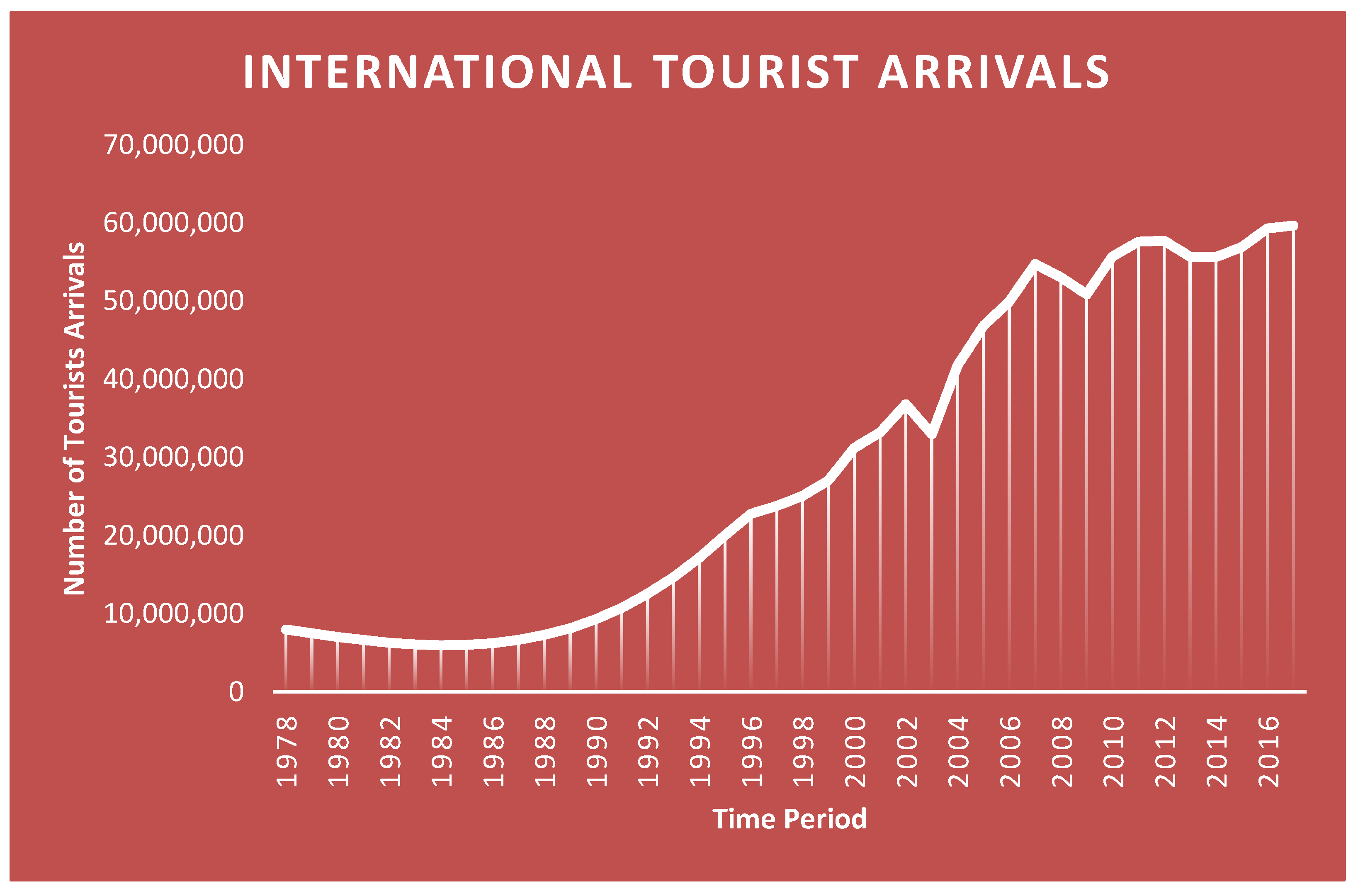
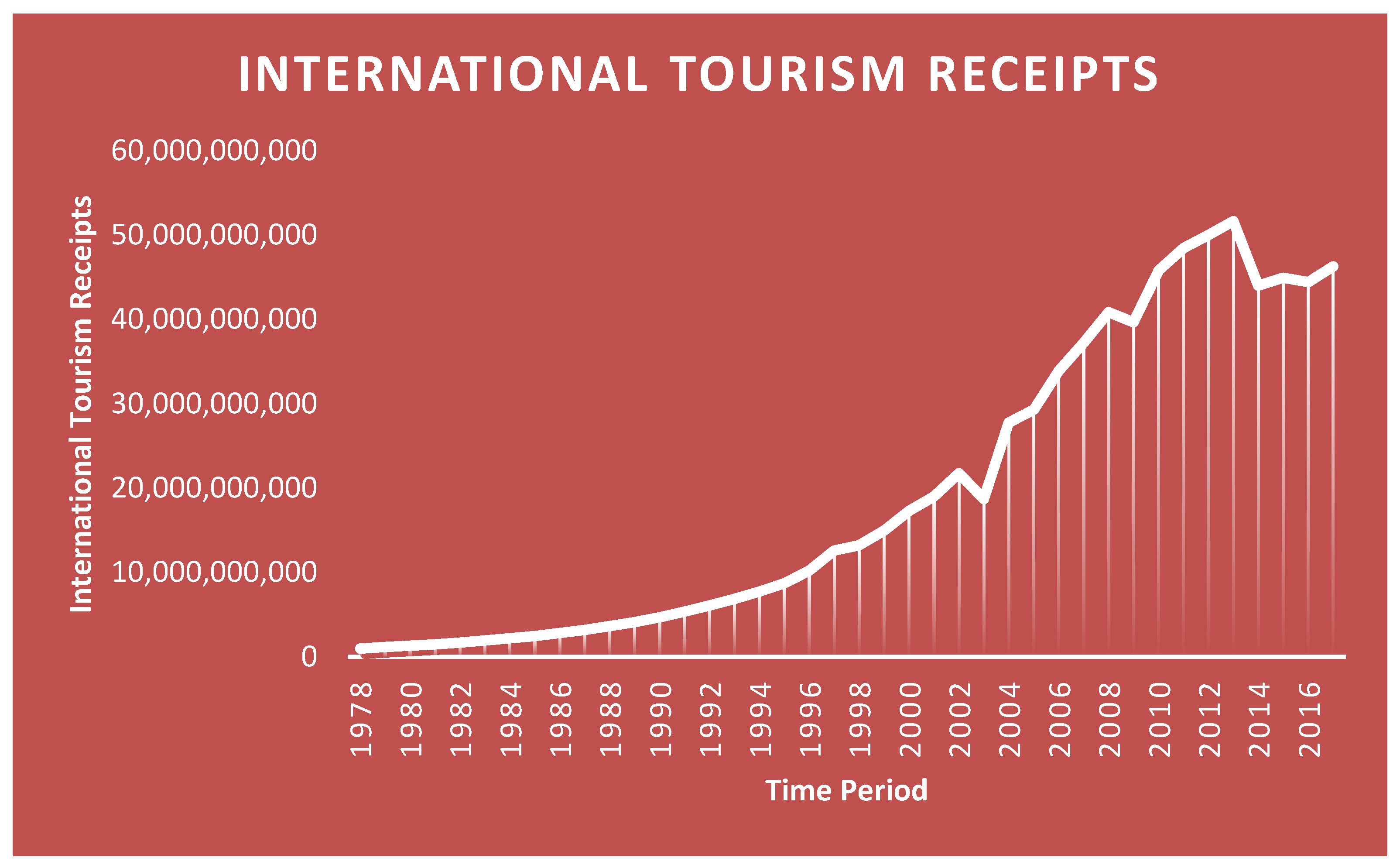
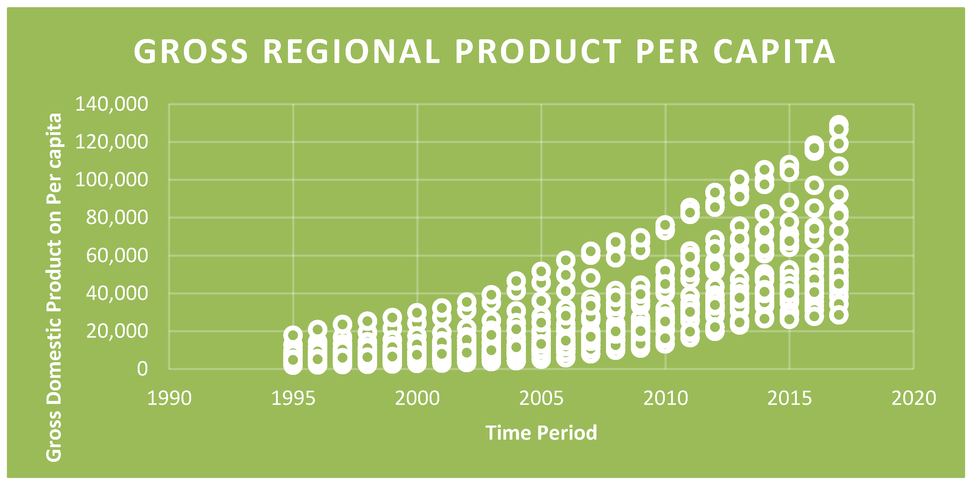
Certainly, the Chinese economy has emerged vibrantly since 1978 until now, as it has made enormous economic progress and undertaken sustainability objectives. However, the immense and fast cumulative level of energy consumption in various industries of China, such as agriculture, services, manufacturing, and the tourism sector, may (unpleasantly) degrade the ecological scenery through CO₂ emissions. Although prior investigations have recognized that tourism is an essential aspect of economic development, where it generates substantial earnings, creates employment opportunities and matures cultural promotion in an economy; on the other hand, it may also be harmful to the environmental quality of that economy. Presently, the tourism sector is positioned globally, and is amongst the sizeable and quickest rising economic segments, due to its substantial contribution to the performance economy. As per the World Travel and Tourism Council (WTTC), the entire contribution of travel and tourism (T&T) to economic progress (GDP) was 8272 billion in 2017, and is projected to increase from 10.4% to 11.7% of GDP in 2028. The exact portion of this segment in GDP was 2570 billion in 2017, and, by the year 2028, it is hoped that this figure will be 3890 billion, e.g., 3.6% of the entire world’s GDP. Presently, the People’s Republic of China is one of the most visited nations, next to Spain, the United States of America, and France, and grossing billions of US dollars per annum as visitor revenues (Figure 1 and Figure 2).

A number of studies have testified that the emission of greenhouse gases (GHGs) has led to serious environmental concerns around the world. The numbers of the International Energy Agency (IEA) indicated that China became the largest CO₂ producer as its volume of CO₂ emission exceeded the USA in 2007 [4]. Recently, the average Earth temperature increased significantly due to the nonstop plunging trend in CO₂ emissions. As a result, significant economies, from developed and developing regions, are adding about 80% of total CO₂ emissions [5,6]. As a part of the modern integrated world, countries are linked with each other through different networks, including energy and power. The reliance between nations pointed in the direction of a common goal and a shared responsibility, to fight for reducing the scale of CO₂ emission. China’s share of global CO₂ emissions stands at around 27% and significantly exceeds the amount of emissions from the USA, at around 16%, with India at the third position, contributing about 7% of the total global emissions. Thus, this massive gap shows that China needs to take serious steps to cut down its share of CO₂ emissions, in order to attain its sustainability and economic goals. Following this pressure, China hopes to reduce its emissions up to 45% by 2020, compared with the 2005 level [7].

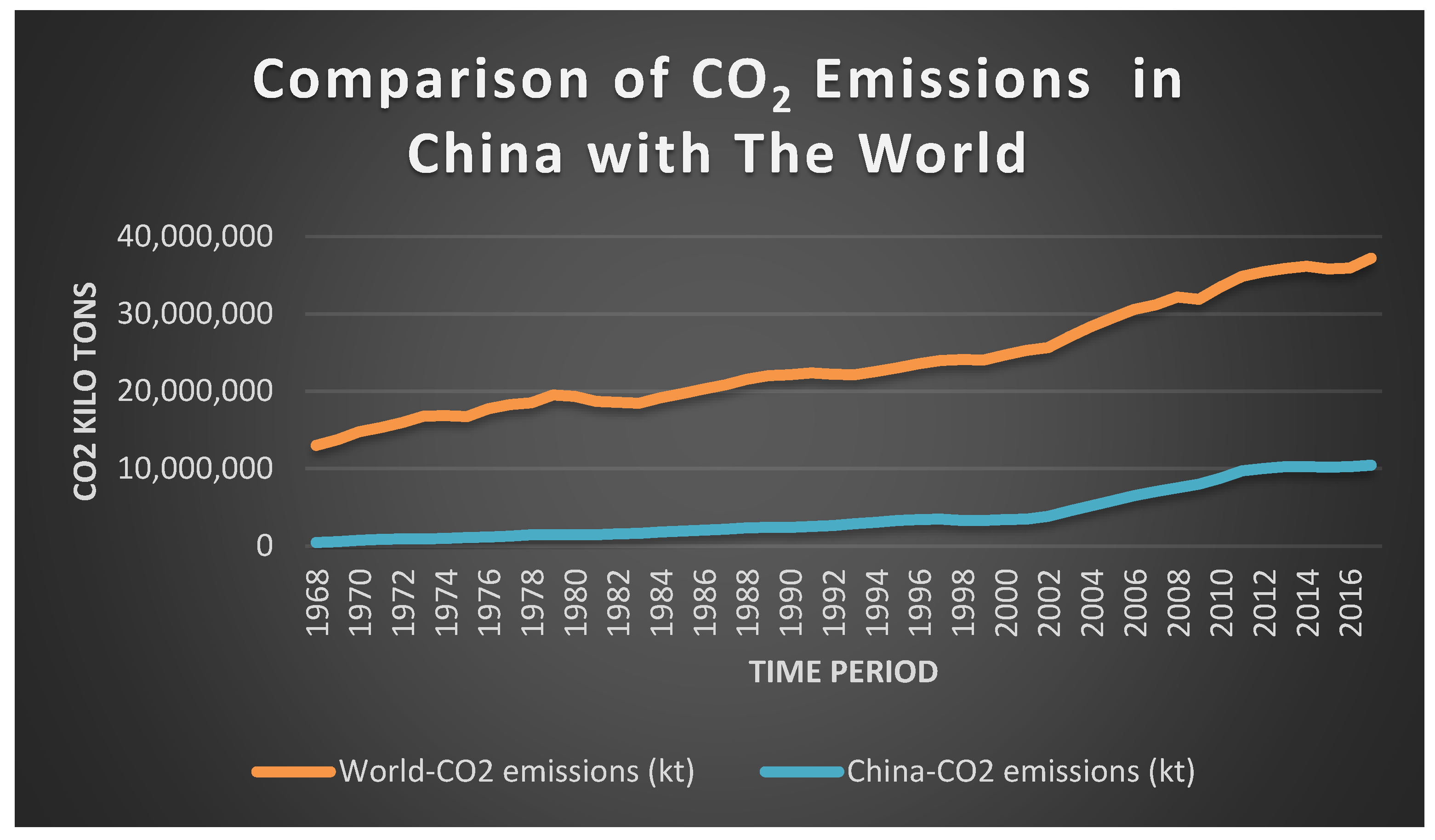
As presented in Figure 3, the comparison of the CO₂ emissions of China with the whole world displays very alarming figures for China, where, from the 1970s to 2016, carbon emissions increased massively and constituted around 30% of the whole world [8]. These facts indicate that China needs to take important measures for sustainable development, by lowering the rate of environmental degradation (CO₂). Taking this recent scenario into account, the Chinese government paid significant attention to this problem. The government proposed “a five in one” plan during the 18th CPC National Congress, to promote cultural, social, political, and environmental construction for the establishment of eco civilized society.

The Chinese government has repeatedly stressed the significance of an eco-civilized society and this issue seeks attention at the national level. Improved environmental quality has been proposed as a form of greater wealth, to improve public awareness. Henceforth, the ecological aspect has been an integral part of the Chinese government’s plan for the sustainable economic progression of China. In fact, as the first report of the IPCC highlighted, CO₂ emission has emerged as a severe threat at an international level, and forming a low carbon green development has become the goal of all nations. Therefore, China has committed to reduce the level of CO₂ emissions for steady domestic and global development. To fulfill this goal, China guaranteed to condense CO₂ per unit of GDP from 60 to 65% by 2030 against the level of CO₂ emission in 2005 [9]. Accordingly, to mature a low carbon economy and cut-back in CO₂ emission has become a great challenge [10,11].

Tourism is one of the most central components of the service industry, and it holds a significant capacity to stimulate the environment due to its rapid growth. The impact of tourism significantly varies, as it can promote cultural and social values and bring people together. On the other hand, tourist activities might significantly influence CO₂ emission [12]. The UNWTO numbers indicate that tourism contributes 4.9% and 1.4% to the global CO₂ emission and global greenhouse effects, respectively. These numbers will grow by 2.5% annually without effective measures [13]. By and large, the CO₂ emissions from the tourism sector can be characterized as direct and indirect emissions. The final energy consumption and related CO₂ emissions is known as direct, while indirect emissions are associated with the production of intermediate goods in this industry. As one of the largest tourist attractions, this industry has been developing rapidly, and China has been experiencing significant numbers of inbound and outbound tourists during recent years. China hosted 129 million tourists, 98 million Chinese tourists went for outbound tourism, and the sum of 3.2 billion local travelers visited during 2013. It is imperative that those traveler movements and processes accompanying this number consume substantial energy stocks and result in a massive level of CO₂ emissions, both directly and indirectly [14,15].

The rapid growth of developing countries and the associated industrial growth are blamed for increased CO₂ emissions [16,17,18]. The tourism led growth phenomena has been accepted, and this remarkable contribution also adds to environmental pollution. Facilities and tourist activities promote energy use and increase the level of CO₂ emissions. However, promoting sustainable tourism can reduce CO₂ emissions [19]. The progress in the tourism sector has both positive and negative impacts, and, ultimately, the native community suffers from these adverse impacts. However, the contribution of this industry can only be increased through the consideration of its encouraging role in climate change, upgrading its environmental quality, and cutting back in CO₂ emissions. Thus, maintaining a balance between the significance of the tourism segment for economic development and its share towards an escalation of CO₂ emission is critical for the Chinese economy, as well as for other developing countries under BRI.

Considering the standing of this sector and its role in environmental quality, the core objective of our research survey is to disclose the long term interconnection between tourism development, transportation, economic progress, energy consumption, and value added hotel and catering services with environmental degradation (CO₂) for a panel of thirty (30) provinces of China over the period of 1995–2017. Primarily, the CD test was applied for glancing at the cross-dependence and, subsequently, the conventional panel unit root tests (IPS, LLC, ADF, PP, and CIPS) were carried out to evaluate the stationarity of the panel dataset series. The dynamic panel modeling, DOLS, FMOLS, and PMG, were run to assess the long term associations among the variables. Additionally, the Granger causality test for panel format was performed to establish a direct relationship between concerned variables. Hence, the retrieved estimates conferred a few guidelines to the Chinese administration at the provincial and national level, such as initiating renewable-based energy projects (solar, wind, and biomass) that may instigate a decline in the usage of fossil fuels energy in industrial, transportation, and hotel and catering service sectors.

The remainder of this paper is systematized as follows: In Section 2 the literature review has been outlined; in Section 3 stands the methodology and data description; Section 4 contains the empirical results and their discussions, and, to conclude, Section 5 shares an ultimate conclusion, recommendations, and future policy implications.

2. Literature Review

A cluster of research studies has been performed to identify the linkages between tourism development, energy utilization (renewable and nonrenewable energy), economic growth, transportation, and carbon emissions around the world, at the national level or at the local level. However, exploring the direction of causality and long-term links between tourism development, the scale of energy consumption, and CO₂ emissions, [20] revealed that tourism development has a positive and momentous effect on the level of carbon emission, although the scale of energy consumption indicated a negative influence on environment status (CO₂ emissions) in Cyprus. The causality test indicated that tourism advancement fosters the scale of energy consumption and CO₂ emission. Bringing into play a balanced panel dataset of developed and less developed nations, León et al. (2014) [21] studied the links between tourism expansion and CO₂ emissions during 1998–2006. The estimates indicated that the expansion of the tourism industry is a key donor to CO₂ emission for both nation groups. However, the shock is more substantial in developed nations than developing ones, and the adoption of a sustainable development path is necessary for the production section to reduce the emission from this industry. Similarly, air travel is also an important subsector that generates greenhouse gases. The results from 11 different tourist countries indicate that there exist significant variations between all countries and destinations regarding the level of CO₂ emission [22]. The study performed in [23] examined the nexus between climate change (CO₂ emissions) and international tourism in the OECD territory. The findings revealed that international tourism has an inverted U-shaped affiliation with CO₂ emissions. Moreover, globalization plays a mediating role in this relationship by eliminating environmental degradation through international tourism. Moreover, [24] examined the secondary data of the entire globe (112 nations) to find out the relationship between tourism, economic development, trade openness, and energy utilization. The examination divides the data into five regional and four income based groups, and found a mixed impact of tourism on environmental excellence for these groups. Nonetheless, findings of the overall data indicated a positive impact of tourism on CO₂ emissions. On the other hand, the investigation carried out by [25] reported that tourism significantly damages environmental quality in Malaysia; whereas, it revealed a negative connection between tourism and environmental degradation for the nations of Singapore and Thailand. The study also reported that governments can play a vital role in the sustainable and environmentally friendly tourism industry.

The study of [26] evaluated the impact of e-tourism on environmental excellence in Saudi Arabia from the period 1995Q1 to 2018Q4. The study formed an e-tourism index by adding the contribution of information and communication technologies (ICTs) to tourism earnings. The examination employed the ARDL model and documented that inbound tourism positively affects CO₂ emissions; although the e-tourism index significantly boosts the GDP in Saudi Arabia. The research conducted by [27] evaluated the imperious role of tourism development in the environmental deprivation of the United States (US), by using the wavelet framework approach, from 1996 to 2015. The outcomes of the wavelet correlation and covariance acknowledged that tourism development positively influences CO₂ emissions, in short, medium, and long term time duration. In addition, wavelet coherence also reported the positive connection of tourism development and CO₂ emissions in these three periods; conversely, the upshots of the continuous wavelet approach exposed stable variance in the long and very long term durations. In order to assess the impact of the tourism industry on climate change, another study, by [28], used the data of the top five carbon emitter nations and divided them into low revenue, lower-middle revenue, high revenue, and upper-middle revenue nations. The outcomes of the analysis reported that tourism has a positive impact on CO₂ emissions for all the groups evaluated in the study but this effect is greater for lower-middle-income nations than high-income countries; whereas it is minimum at the global level.

Rauf et al. (2018a, 2018b) [6,29] argued that there are substantial, momentous drifts of various economic indicators, such as urbanization, energy usage, financial development, and gross fixed capital formation, to ravage the environment at a multinational, regional and local levels of the Belt and Road Initiative (BRI) nations. Therefore, to reduce the extent of nonrenewable energy consumption (fossil fuel energy) and deflate its worsening impacts on the environment, landscape could be an additional font for defending the future environmental challenges, especially for China and in BRI clustered countries in general. Similarly, Rauf et al., (2018) [16] discovered, for China, that the growth of the sector had been considered as a contributor to the amplification of the intensity of carbon emissions (detriment to environment sceneries) regarding trade openness, energy consumption, and urbanization from 1978 to 2017. Hence, the robust laws and actions to rheostat the intensity of (CO₂) emission in China, and address in a way of the green economy may hold back to the environmental status properly.

A recent study was performed by using decomposition analysis to compute the level of (CO₂) emission for Portuguese tourism activities. Moutinho et al. (2015) [30] observed that energy, labor productivity, fixed capital, and the tourism industry have important effects on overall carbon emission. The degree of energy consumption and tourist activities have a significant impact on carbon (CO₂) emission through the accommodation, food, recreation, and transport sectors. During the period of turmoil, tourism supported the Portuguese economy and boosted sustainable development with its significant contribution. At the same time, the environmental aspect of tourism cannot be neglected. Examining CO₂ emissions and their impact on tourism, Robaina-Alves et al. (2016) [31] outlined five (5) subsectors of that industry that are indispensable in order to deal with CO₂ emissions. This sector influences the emissions level with the total energy consumption intensity. Using the monthly data from the USA, Raza et al. (2017) [27] confirmed the positive and substantial effect of tourism on CO₂ emission. The linkage is effective in the short, medium, and long term and unidirectional causality runs between both factors during the period of the analyses.

Sharif et al. (2017) [32] searched for the linkages between tourism sector enlargement and the degree of CO₂ emissions in Pakistan. The estimates from several econometric methods confirm a long term interrelationship between both featured variables. Furthermore, the variance decomposition analysis (VDA) shows a unidirectional causality passing from tourism development to CO₂ emissions, which illuminates that more efforts are necessary to motivate the involvement of this sector in the economic progress of Pakistan. Considering a panel dataset of certain Asian Pacific nations, [33] scrutinized an interconnection between economic expansion, tourism sector enlargement, energy utilization, and the extent of CO₂ emissions. The interrelationship between the number of tourist arrivals and the quantity of CO₂ emissions is positive and significant, and the causative relationship between the number of tourist arrivals, energy utilization, and CO₂ emissions are also noteworthy. Analyzing the closeness between CO₂ emission, energy usage, real GDP and tourism progression for the EU and contender nations, [34] intimated a long-term tie between the variables. The outcomes from dissimilar estimates authorized that energy usage increases the level of CO₂ emissions; however, income and tourism reduce this level. The causal relationship indicates a bidirectional coupling between energy usage and CO₂ emissions, and one way ties between tourism expansion and degree of CO₂ emission.

It is richly documented that tourism progression contributes to economic growth; however, the increased amount of CO₂ emissions from tourism related activities adds to environmental degradation. Exploring the link between CO₂ emissions caused by tourist arrivals and environmental pollution, [25] publicized that tourism advancement has a positive and substantial impact on CO₂ emission in Malaysia. Despite this, this connection is negative for Singapore and Thailand, which suggests that environmentally and socially responsible tourism reduces pollution issues. Scanning the footprint of the relationship between tourism expansion, economic progress, and the level of CO₂ emission in a multivariate milieu by tapping afresh a familiarized globalization index, Akadiri et al. (2018) [35] found that internal factors are more influential on the association of variables for small island developing countries. Investigating the influence of tourism outlay on tourism growth, and its influence on CO₂ emission for the EU nations, [36] confirmed an established relationship between the variables. The results showed the positive effect of capital spending in the sightseeing industry on tourism proceeds, and an adverse impact on CO₂ emissions, with a dual way causality between investments and tourism sector enlargement. This suggests that tourism investment not only increases revenues but also lowers the level of carbon emissions. Analyzing the leading sources of carbon emissions by way of tourism activities in Barcelona city, [37] cited that the direct and indirect emissions from tourism events increased in Barcelona city. The principal source of CO₂ emissions is arrival and departure transportation, which generates 95% of the total emission. Thus, the government needs to apply strict policy measures to control emissions from the transport and housing sectors.

Taking the case study of Chengdu, the largest city in terms of tourism output in western China, [38] observed energy needs and usage, and its effects on intended CO₂ emissions in the tourism sector. The end result signals that, in general, the level of energy utilization and CO₂ emission increased during 1999–2004. The transportation sector heavily contributes toward power utilization and CO₂ emissions. The immersion of this sector is relatively more important than the food and entertainment sectors. In addition, energy concentration, outflow magnitude, and business mass are critical factors to stimulate the scale of energy consumption and emissions from tourism activities. The tourism sector of China has undergone a rapid expansion, and, as a result, the level of CO₂ emissions increased correspondingly. Exploring the CO₂ emissions from the tourism industry of China, [39] identified that wide ranging CO₂ emissions have noticeably increased during the period of 1990 to 2012. The transportation sector is the most significant contributor to CO₂ emissions, consuming 80% of the total share. Generally, the contribution of tourism to an economy is higher than the relative level of CO₂ emissions. There is a growing gap between the tourism based emissions for different sectors, and the transport sector is the most prominent contributor to emissions.

Using the regional data, [40] investigated the long term and short-term associations between the sightseeing industry, economic escalation, and CO₂ emissions. The findings of the multivariate context underwrote that the EKC hypothesis is incompetently underpinned in Chinese regions. There is significant evidence for tourism led growth in the long term, however, causality conflicts among regions. Overall, in the long term, an expansion of tourism has a noteworthy impact on economic progress and carbon emissions, and a bidirectional causal binding endured between economic development and the scale of CO₂ emission in three regions. Ahmad et al. (2018) [19] studied the five provinces of the western region in China, and concluded that the impact of the expansion of tourism on the ecosystem is unfavorable in Gansu, Ningxia, Shanxi, and Qinghai, but tourism progress improves the environmental conditions in Xinjiang. Thus far, the damaging impact of economic progress and energy usage is more noteworthy than tourism growth on carbon emission over the long term. Evaluating the direct and indirect emissions from tourism activities for Hubei (China), [14] unearthed that the aggregate of CO₂ emissions inflated from 2007 to 2013, with transportation at the top, generating more than 50% of the total. The share of accommodation and other service sectors is lower than transportation. Indirect emissions increased significantly from transportation, but the level is much lower for other secondary sectors.

Furthermore, the efficiency of promoting a low carbon economy varies among cities and remains lower than the expected level. However, the overall shift of focus to efficiency increased within the sample period. Zhang and Zhang (2018) [41] advised that a carbon tax policy can contribute significantly towards economic development and lower the scale of CO₂ emissions from the tourism business in China. The effect of these taxes varies from time to time, and the significance of various tourism sectors also differs, depending on internal policies.

By reviewing the prevalent writings, it is evident that the erstwhile research writings waived the BRI associated objectives and potentials for China in the region of tourism development, and how tourism development, transportation, and economic growth can ease the intensity of ecological degradation. Accordingly, China, as the setter of BRI, needs to mitigate massive challenges at the national and international levels, such as taking BRI as a gainful opportunity in which the tourism industry can thrive, cultural diversification, tethering trade partnerships, infrastructural development through roads and railways, sustainable growth and significant energy production and consumption frameworks. Therefore, it is required to make sound policies and actions for Chinese provinces to expand the scale of economic and tourism development by shrinking the devastating impacts on their environmental sceneries. Similarly, at present, every economy is on a mission to establish an optimal approach for balancing its energy demand and supply, and achieving sustainable development without disturbing its environmental setup. Thus, the present research manages to corroborate the nexus between tourism expansion, transportation, economic progress, energy usage, and environmental pollution in thirty (30) provinces of China, in light of BRI challenges and panoramas.

3. Materials and Methods

Indeed, China is performing a dominant role in the world’s economic growth, but the commencement of the Belt and Road Initiative (BRI) has been the main contributor to its substantial importance around the world. The main focus of BRI is integrating with the partner countries for cooperation, sharing cultural versatility, strategical contacts, infrastructural development, and economic cooperation. Similarly, the Chinese government has taken this initiative as an opportunity to promote tourism within and outside China, considering climate change and ecological issues. Thus, China needs to address the issues of dismantling, related to environmental quality, promoting the tourism sector in various regions of China under the “New Normal” phase.

3.1. Data

The dataset material in

Table 1. Variable metaphors and dataset informers.

Variables Label	Computing Units and Their Comprehension	Dataset Informers
Carbon emission (CO2)	(10,000) Tons of CO2 Emissions from Coal, Gas, and Oil	NBS/WDI
Energy consumption (ECON)	Energy Utilization of Unit GRP (Equivalent value)	NBS/WDI
Gross domestic product (GDPPC)	Per Capita Gross Regional Product (RMB/person)	NBS/WDI
Hotel and Catering Services (VHCS)	Value of Hotels and Catering Services (RMB 100 million)	NBS/WDI
Tourism Development (TD)	PCA index Tourism Receipts and Tourist arrivals	NBS/WDI
Transportation (TRANSP)	PCA index of the length of Railway, Highways and Passenger traffic (10,000)	NBS/WDI

Note: Author’s tabulation; Source: National Bureau of Statistic (NBS) of China/World Bank Development Indicators (http://data.stats.gov.cn/english/adv.htm?f=aq&cn=E0103&nodeid=900001&wdcode=reg) (accessed on 16 August 2019).

has been collected from the World Development Indicators [42], as well as from Chinese databases (the National Bureau of Statistics (NBS) of China and Statistical Yearbooks for China) [43]. The collected dataset was, in nature, balanced panel data that included 30 Chinese provinces, in

Table 2. List of the 30 Provinces of China.

Sr. No	Country	Sr. No	Country	Sr. No	Country
1	Beijing	11	Anhui	21	Hainan
2	Hebei	12	Zhejiang	22	Sichuan
3	Tianjin	13	Jiangxi	23	Chongqing
4	Inner Mongolia	14	Fujian	24	Yunnan
5	Shanxi	15	Henan	25	Guizhou
6	Jilin	16	Shandong	26	Gansu
7	Liaoning	17	Hunan	27	Shaanxi
8	Heilongjiang	18	Hubei	28	Ningxia
9	Jiangsu	19	Guangxi	29	Qinghai
10	Shanghai	20	Guangdong	30	Xinjiang

Source: National Bureau of Statistic (NBS) of China/World Bank Development Indicators (http://data.stats.gov.cn/english/adv.htm?f=aq&cn=E0103&nodeid=900001&wdcode=reg) (accessed on 16 August 2019).

, ranging from 1995 to 2017, the excluded provinces are: Tibet and other regions such as, Hong Kong, Macao, and Taiwan, due to unobtainability of the dataset and some other limitations [40] Energy consumption is as GRP units (correspondent value).

The recent study engages CO₂ emissions kilotons (kt) as A predicted variable, while gross domestic provincial revenues, represented as GDPPC, energy consumption with ECON, as used by [20,44], and value-added hotel and catering services (VHCS) are considered as a proportion of GDPPC for hoteling services. Principal component analysis (PCA) is engaged to compute tourism development (TD) in light of tourism receipts in USD millions and number of overseas tourist arrivals [34,40,45]. Similarly, for transportation (TRANSP), a PCA index is designed which covers the length of railway operations, length of highways in 10,000 km, and passengers’ traffic in 10,000 persons, in Table 1. In this research assessment, overall energy consumption (kt of oil equivalent) and CO₂ emission (kt) are used to characterize energy usage and climatic change or environmental pollution, respectively.

In Table 2, there has been stated a list of provinces, on those our current investigation is prevailing and insights for Chinese economy are obtained, with the aim of future challenges and prospects, by considering BRI as a remarkable breakthrough. Meanwhile, the dataset for CO₂ emissions was also robust, checked from the World Bank Database (2018) [46], to ratify its portrayal and calculations. Given that, CO₂ emissions for 30 provinces are unavailable on NBS, China, thus, in light of the Intergovernmental Panel on Climate Change (IPCC) (The dataset for CO₂ emissions for 30 provinces is not available on NBS, China. Thus, Emissions for CO₂ is calculated under IPCC, 2006, provided a formula for CO₂ estimations. The equation could be written as: (CO₂ $=\sum _{\mathrm{i}=1}^3\frac{{\mathrm{E}}_{\mathrm{i}}}{{\mathrm{a}}_{\mathrm{i}}}{\mathsf{\beta }}_{\mathrm{i}}$), where CO₂ characterizes CO₂ emissions;${ \mathrm{E}}_{\mathrm{i}}$ symbolizes energy consumption through three sources: coal, oil, and natural gas consumption; ${\mathrm{a}}_{\mathrm{i}}$ designates conversion rate for energy consumption through coal, natural gas and crude oil; and ${\mathsf{\beta }}_{\mathrm{i}}$ implies the level of CO₂ emission factors for each of the three fuels. The rate for conversion from the three fuels to standard coal are in this manner: 1 kg of coal consumption = 0.7143 kg of standard coal; 1 kg crude oil = 1.4286 kg of standard coal; and 1 m³ natural gas = 1.33 kg of standard coal. Hence, the resulting factors of CO₂ emission for crude oil, coal, and natural gas are 3.12 t/m³ 1.86 t/m³, and 0.00209 t/m³, respectively), the computation for provincial amassed level CO₂ emissions have been functioned by multiplying the carbon emission elements with a sum-up of coal, gas and crude oil consumption for energy (in kg of the orthodox level of coal), as bi-variate model blueprints are opposed by various researchers for their inefficiency and biased estimation. Hence, the on-hand study collects these circumstances and elaborates an interrelationship between tourism development, as tourism proceeds, the size of tourist inflows, and the level of CO₂ emissions. Likewise, transportation is also a big contributor to enlarging the scale of CO₂ emissions, so it is used as an exogenous economic indicator. Besides these, there were other controlled variables used, such as GDPPC, VHCS, and ECON for causality bonding among the subjected variables. In Figure 4, the gross domestic provincial product (GDPPC) pattern has been identified among the 30 provinces from 1995 to 2017. This has clarified that regional output is increasing year by year; likewise, the level of CO₂ emissions in provinces also have an upward trend. The pattern of CO₂ emissions among the 30 provinces of China from oil, gas, and coal, are given in Figure 5.

3.2. Methodology and Model Identification

As equivalent to [20,34,40,44,45], the on-hand investigation benefits from the following function, where an equation could be specified as follows:

$${\mathrm{CO}}_2=\mathrm{f} (\mathrm{TD}, \mathrm{GDPPC}, \mathrm{ECON}, \mathrm{VHCS}, \mathrm{TRANSP})$$

(1)

In the aforementioned Equation (1), CO₂ emissions are described as a predicted variable and tourism development (TD) (number of tourists’ arrivals and tourism receipts), gross domestic product (GDPPC), energy consumption (ECON), value-added hotel and catering services to gross regional product (VHCS), and transportation (TRANSP) (length of railways, highways, and passenger traffic 10,000), are the predictor variables. Standardization and conversion of the dataset is an important aspect to stabilize the dataset ranges and transfigure all the variables, based on their specification, into natural logarithms, which will support the avoidance of irregularities linked with dynamic properties of the panel datasets [34,40,45]. The log conversion of dataset ranges is an ideal process, as each significant coefficient value in regression scrutiny can be judged as movements in the direction of the predictor variable. Hence, the following, Equation (2) is detailed as follows:

$${\mathrm{CO}}_{2\mathrm{i},\mathrm{t}}=\mathsf{\alpha }+{\mathsf{\beta }}_1{\mathrm{lnTD}}_{\mathrm{i},\mathrm{t}}+{\mathsf{\beta }}_3{\mathrm{lnGDPPC}}_{\mathrm{i},\mathrm{t}}+{\mathsf{\beta }}_2{\mathrm{lnECON}}_{\mathrm{i},\mathrm{t}}+{\mathsf{\beta }}_4{\mathrm{lnVHCS}}_{\mathrm{i},\mathrm{t}}+{\mathsf{\beta }}_5{\mathrm{lnTRANSP}}_{\mathrm{i},\mathrm{t}}+{\mathsf{\epsilon }}_{\mathrm{i},\mathrm{t}}$$

(2)

The exemplification in Equation (2) unveiled the forecasted variable and forecasting regressors; “$\ln$” advocates a natural logarithm; the signs of “i” and “t” denote province specific information and time in the dataset, consistently. Furthermore, “α” is a panel equation intercept; β illustrates coefficients for the forecasting variables of the entire study, an “${\mathsf{\epsilon }}_{\mathrm{i},\mathrm{t}}$” is the innovativeness or residuals term in the subjected study.

3.2.1. Panel Unit Root Tests

Before spotting the stationarity properties of CO₂, TD, GDPPC, VHCS, TRANSP, and ECON, the features of the panel dataset should be expanded with the aim of employing suitable panel unit root assessment tests for the present investigation. In any event, where the panel dataset is not identically homogeneous and cross-sectionally self-determining, the traditional panel unit root assessing tests, such as LLC, IPS, ADF, Hadri, and PP, devised by [47,48,49,50,51], may yield unreliable and malfunctioning outcomes.

As per an anticipated dependence amid 30 province-based panels of China for CO₂, TD, VHCS, TRANSP, GDPPC, and ECON economic pointers, the present study will utilize the cross-section dependence (CD) test familiarized by Pesaran (2004) [52] to evaluate the degree of residuals in provinces cross-sectionally, and their dependence with each other. Likewise, the situated dependency in variables is enlarged in several ways, such as some unnoticed joint components may be absent and in line with other spatial reliances (dependence). Accordingly, the Pesaran’s CD measurement tool is also an appropriate device, on occasion of a smaller T and greater N; however, counting the stationarity, unit root dynamic tests, and heterogeneous in spatial economic models. The test for CD devised by [52] can be expressed in this fashion:

$$\mathrm{CD}=\sqrt{\frac{2\mathrm{T}}{\mathrm{N}\left(\mathrm{N}-1\right)}}\left({\displaystyle \sum }_{\mathrm{i}=1}^{\mathrm{N}-1}{\displaystyle \sum }_{\mathrm{j}=\mathrm{i}+1}^{\mathrm{N}}{\hat{\mathsf{\rho }}}_{\mathrm{ij}}\right)~ \mathrm{N}\left(0,1\right)\mathrm{i}, \mathrm{j}=1,2,3\dots 30\dots \mathrm{N}$$

(3)

where ${\hat{\mathsf{\rho }}}_{\mathrm{ij}}$ denotes the residual based pairwise correlation sample evaluation that has been originated from ADF linear regression equations. To certify the long-term connection amongst the variables (CO₂, TD, VHCS, TRANSP, GDPPC, and ECON) in the panel, it is mandatory to perform a test for panel unit root preceding the cointegration test. As per, proper panel unit root tests are relied upon for initial screening, to determine whether provinces in China (30) have cross-sectional dependence or independence over the period [6,53,54]. Hence, the current study will employ parametric (2nd generation) as well as nonparametric (1st generation) panel unit root tests, to obtain solidarity outcomes for additional concluding annotations for the developing world’s economies. The ending results from the above equation have been concluded for all the subjected variables in

Table 3. Cross sectional dependence test.

Pesaran’s CD Values	CO2	TRANS	TD	GDPPC	VHCS	ECON
Statistics	88.4257 ***	66.5017 ***	75.3804 ***	99.4713 ***	99.6817 ***	96.7161 ***
Probability-value	0.0000	0.0000	0.0000	0.0000	0.0000	0.0000

*** Denotes the statistical significance at 1% level. This test assumes the null hypothesis of cross-section independence.

, individually.

The second generation panel unit root test of Pesaran’s is healthier in its features, owing to the asymptotic assumption, and does not compel for N→∞. Thus, the Pesaran’s test is an annex of the CIPS test that may be framed as follows:

$$\Delta {\mathrm{y}}_{\mathrm{i},\mathrm{t}}={\mathrm{c}}_{\mathrm{i}}+{\mathsf{\alpha }}_{\mathrm{i}}{\mathrm{y}}_{\mathrm{i},\mathrm{t}-1}+{\mathsf{\beta }}_{\mathrm{i}}{\overline{\mathrm{y}}}_{\mathrm{t}-1}+{\displaystyle \sum }_{\mathrm{j}=0}^{\mathrm{p}}{\mathsf{\gamma }}_{\mathrm{ij}}\Delta {\overline{\mathrm{y}}}_{\mathrm{i},\mathrm{t}-\mathrm{j}}+{\displaystyle \sum }_{\mathrm{j}=1}^{\mathrm{p}}{\mathsf{\delta }}_{\mathrm{ij}}\Delta {\overline{\mathrm{y}}}_{\mathrm{i},\mathrm{t}-\mathrm{j}}+{\mathsf{\eta }}_{\mathrm{i},\mathrm{t}} \mathrm{i}=1,\dots \mathrm{n}$$

(4)

The above Equation (4) elaborates that, ${\mathrm{c}}_{\mathrm{i}}$ is the deterministic tag, $\overline{\mathrm{y}}$ characterizes the cross-sectional average for $“\mathrm{t}”$, time, and the lag operator is displayed with $“\mathrm{p}”$. Suppose ${\mathrm{t}}_{\mathrm{i}}$ (N, T_m) symbolizes the matching t-ratio of ${\mathrm{a}}_{\mathrm{i}}$ At that moment, the mean value of t-ratios is posed in this manner:

$$\mathrm{CIPS}\left(\mathrm{N},{ \mathrm{T}}_{\mathrm{m}}\right)=\frac{{\sum }_{\mathrm{i}=1}^{\mathrm{N}}{\mathrm{t}}_{\mathrm{i}, }\left(\mathrm{N},{ \mathrm{T}}_{\mathrm{m} }\right)}{\mathrm{N}}$$

(5)

Accordingly, the captured panel dataset proposes that a greater number of time occasions may nurture a degree of freedom (DoF), subsequently, the stated condition would be rooted in multicollinearity and autocorrelation setbacks in the panel ordinary least square (OLS) equation. Therefore, the unit root test in the context of IPS and LLC is justified by succeeding equation modeling as:

$$\Delta {\mathrm{y}}_{\mathrm{i},\mathrm{t}}={\mathrm{\alpha }}_{\mathrm{i}}+{\mathsf{\beta }}_{\mathrm{i}}{\mathrm{y}}_{\mathrm{i},\mathrm{t}-1}{\displaystyle \sum }_{\mathrm{j}=1}^{\mathrm{pi}}{\mathsf{\rho }}_{\mathrm{ij}}\Delta {\mathrm{y}}_{\mathrm{i},\mathrm{t}-\mathrm{j}}+{\mathsf{\epsilon }}_{\mathrm{i},\mathrm{t}} \mathrm{i}=1,\dots \mathrm{t}=1,\dots \mathrm{T}$$

(6)

Equation (6) has been integrated, ${\mathrm{y}}_{\mathrm{i},\mathrm{t}}$ as a panel dataset cross-section with “$\mathrm{i}$” (provinces) and time “$\mathrm{t}$”over the period, “${\mathsf{\rho }}_{\mathrm{i}}$” specifies the lag operator for above mentioned Equation (5). Furthermore, “${\mathsf{\epsilon }}_{\mathrm{i},\mathrm{t}}$” enumerates the innovation and time for each province in China to normalize the random dispersal of dependent and independent variables. Accordingly, two hypotheses have been established, the null and alternative, to trace the feature of stationarity among the variables with four unalike panel unit roots assessment tests (LLC, IPS, ADF, and PP). Where ${\mathrm{H}}_0$ = null hypothesis for the entire panel, with $\mathrm{p}$ = 0 for the province “i” (panel dataset variables having a unit root in their distribution); in contrast $\mathrm{p}$ < 0 represents ${\mathrm{H}}_1$ = alternative hypothesis, when the lowest value is one or less in province “i” (the panel series does not hold a unit root). Correspondingly, there will be acceptance and rejection for a hypothesis based on its asymptotically determined tabulated statistics.

3.2.2. Panel Cointegration Tests

To be in harmony with panel unit root estimates from the 1st and 2nd generations, a series is stable at level I (0) or in first difference I (1). Accordingly, the next phase is to consider the level of cointegrating linkages between the variables. Thus, if two variables are disjointedly non-stable but holding the same pattern, and their movement with each other is in the same direction or together, then it determines that cointegration (1, 1) is prevailing among them.

Hence, to test the level of cointegration between the variables, the Pedroni test for cointegration has been calculated [55,56] to measure the cointegrating pattern among the studying variables, as exemplified by [29,57,58]. The Pedroni test for cointegration is made up of seven residuals, established by arithmetical assessment tests to identify the existence of long-term connectedness among the variables. The first four panel statistics within the dimension are: panel v-statistic, panel rho-statistic, panel ADF-statistic, and panel PP-statistic. Meanwhile, based on groups and between dimensions are: group intensive rho-statistics, group ADF-statistics, and group PP-statistics values. An equation for the Pedroni cointegration test is as follows:

$$\begin{gathered} {\mathrm{CO}}_{2\mathrm{i},\mathrm{t}}={\mathsf{\alpha }}_{\mathrm{i}}+{\mathsf{\delta }}_{\mathrm{i}}\mathrm{t}+{\mathsf{\beta }}_1{\mathrm{lnTD}}_{\mathrm{i},\mathrm{t}}+{\mathsf{\beta }}_2{\mathrm{lnGDPPC}}_{\mathrm{i},\mathrm{t}}+{\mathsf{\beta }}_3{\mathrm{lnECON}}_{\mathrm{i},\mathrm{t}}+{\mathsf{\beta }}_4{\mathrm{lnTRANSP}}_{\mathrm{i},\mathrm{t}}+{\mathsf{\beta }}_5{\mathrm{lnVHCS}}_{\mathrm{i},\mathrm{t}}+{\mathsf{\epsilon }}_{\mathrm{i},\mathrm{t}} \\ \mathrm{here} \mathrm{i}=1,\dots \mathrm{t}=1,\dots \mathrm{T} \end{gathered}$$

(7)

In Equation (7) cointegration demonstration has been represented for: “${\mathsf{\alpha }}_{\mathrm{i}}$” is the provincial specific constant, and the tendency of the deterministic is shown as “${\mathsf{\delta }}_{\mathrm{i}}\mathrm{t}$” for matching every single province in the full panel for China. The null hypothesis is created as

Hypothesis 1 (H1).

There is a cointegration memory among the variables for “i” provinces.

Alternatively,

Hypothesis 2 (H0).

There is no cointegration memory among the variables for “i” provinces.

Hence, if first four panel statistics contained a greater positive value as per their power, and, on the contrary, the statistics determine a larger negative value as per their weight, then “H0” will be discarded and it will be inferred that there is a long term cointegration found between variables. The formation for the Pedroni cointegration equation could be as below:

$$\sqrt{\frac{{\mathrm{N}}_{\mathrm{N},\mathrm{T}}^{’}-\mathsf{\mu }\sqrt{\mathrm{N}} }{\sqrt{\mathrm{V}}}}\to \mathrm{N} \left(0,1\right)$$

(8)

In Equation (8), it is disclosed that $\mathsf{\mu }$ and $\mathrm{V}$ denote Monte Carlo (MC) fashioned simulation and disparity.

Furthermore, two cointegration techniques, such as the Johansen cointegration [59] and the Kao based cointegration tests [60], based on ADF, are operated to authorize estimates for the Pedroni cointegration test. All three tests’ estimates located the presence of long term cointegration in the data variables. Accordingly, the Pedroni, Johansen and Kao tests of cointegration are residual based and fix the asymptotically natural dispersal by undertaking no co-integration under the null hypothesis. However, these three tests for cointegration may not appropriately capture the cross-sectional dependence delinquent and sourcing for loss of power in recognizing the co-integration nexus amongst the panel dataset for China. Thus, to conclude the level of co-integration in the concerned variables, the Westerlund (2007) co-integration test is the best choice from the aforesaid cointegration tests in the presence of cross-section dependence among the forecasted and forecasting variables [6,61,62].

Since the long term cointegration exists in the recent study, then it will engage the panel fully modified OLS (PFM-OLS), as well as the dynamic OLS (D-OLS) Pedroni, (2000, 2001) [63,64], to evaluate the long-term connection among the regressors and forecasted variables. The key impetus for realizing the dynamic models (PFM-OLS and D-OLS) is allowing for correlational impediments amongst the panel intensive residuals. As a result, all considered variables are converted into a natural log structure to normalize the outcomes. The following PFM-OLS and D-OLS equations will ascertain a long term nexus among the variables, as shown below:

$${\hat{\mathsf{\beta }}}_{\mathrm{NT}}=\left[\frac{{\sum }_{\mathrm{i}=1}^{\mathrm{N}}{\sum }_{\mathrm{t}=1}^{\mathrm{T}}\left({\mathrm{x}}_{\mathrm{it}}-{\overline{\mathrm{x}}}_{\mathrm{i}}\right)\left({\mathrm{y}}_{\mathrm{it}}-{\overline{\mathrm{y}}}_{\mathrm{i}}\right)-\mathrm{T}{\hat{\mathsf{\gamma }}}_{\mathrm{i}}}{{\sum }_{\mathrm{t}=1}^{\mathrm{T}}{\left({\mathrm{x}}_{\mathrm{it}}-{\hat{\mathrm{x}}}_{\mathrm{i}}\right)}^2}\right]$$

(9)

where,

$${\hat{\mathsf{\gamma }}}_{\mathrm{i}}={\hat{\mathsf{\Gamma }}}_{21\mathrm{i}}+{\hat{\mathsf{\Omega }}}_{21\mathrm{i}}^0-\frac{{\hat{\mathsf{\Omega }}}_{21\mathrm{i}}}{{\hat{\mathsf{\Omega }}}_{21\mathrm{i}}}\left({\hat{\mathsf{\Gamma }}}_{22\mathrm{i}}+{\hat{\mathsf{\Omega }}}_{22\mathrm{i}}^2\right)$$

(10)

and

$${\hat{\mathsf{\Omega }}}_{\mathrm{i}}={\hat{\mathsf{\Omega }}}_{\mathrm{i}}^0+{\hat{\mathsf{\Gamma }}}_{\mathrm{i}}+{\hat{\mathsf{\Gamma }}\prime }_{\mathrm{i}}$$

(11)

The symbol ${\widehat{?}}_{\mathrm{i}}$ determines the matrix for long term stationarity, followed by ${\hat{\mathsf{\Omega }}}_{21\mathrm{i}}^0$ which allocates covariance amongst the stationary residuals. Additionally, ${\widehat{?}}_{\mathrm{i}}$ exemplifies the amended covariance term between the regressor variables.

3.2.3. Heterogeneous Panel Causality Test

The following segment is to figure out a granger causative investigation among the variables. The Dumitrescu–Hurlin panel heterogeneous causality test, pronounced by Dumitrescu and Hurlin (2012) [65], is set upon Wald asymptotical statistics for short term causatives. The test appears to be fitting for apprehending the heterogeneity problem in the pairwise Granger based nexus. Therefore, the Dumitrescu–Hurlin panel causality test is fostered on two unlike statistical values, such as Zbar statistics and Wbar statistics. However, Zbar statistics stage a standard normal dispersion, while Wbar statistics take on mean based statistics in the subjected test. The panel heterogeneous causality test is composed of the null and alternative hypotheses, where “H0” typifies a null hypothesis and “H1” denotes an alternative hypothesis.

Hypothesis 1 (H1).

βi = 0 ^I = 1,…,N (there is a causal linkages from x to y).

Hypothesis 2 (H0).

βi = 0 ^i = 1,…,N1;βi ≠ 0 ^i = N1+1,N1+2,…, N (there is no causal linkages from x to y)

4. Empirical Results and Discussions

In the first instance, the descriptive summary statistics are presented in

Table 4. Descriptive statistics.

Variable	Obs	Mean	Std. Dev.	Min	Max	Skewness	Kurtosis
CO2	690	25,450.33	23,421.3	0.0000	128,888	1.65811	5.89642
TRANS	690	−6.57 × 10−10	1.00001	−1.0212	7.93013	2.82045	16.9596
TD	689	8 × 10−10	1.000	−0.4697	7.81737	5.56395	38.0421
GDPPC	690	25,719.61	23,827.8	1826	128,994	1.55146	5.47539
VHCS	690	210.0361	294.648	0.0000	1665.39	2.0927	7.96324
ECON	689	0.4334543	0.77122	0.0000	4.14	1.97463	6.88129

Note: Author’s presentation where CO₂ symbolizes carbon emissions; GDPPC illustrates gross domestic product per capita; ECON describes energy consumption; TD represents tourism development; TRANSP designates transportation, and VHCS signifies value added for hotel and catering services. Furthermore, Std. Dev. represents standard deviation, and Obs. denotes the number of observations.

, for the 30 provinces of China, the correlational statistical matrix in

Table 5. Correlational statistics.

Correlation	CO2	TRANS	TD	GDPPC	VHCS	ECON
CO2	1
TRANSP	0.3893	1
TD	0.1793	0.562	1
GDPPC	0.2643	0.1678	0.3654	1
VHCS	0.513	0.5513	0.5824	0.6614	1
ECON	0.15	0.0279	−0.0471	−0.0757	−0.0372	1

Note: Author’s presentation where CO₂ symbolizes carbon emissions; GDPPC illustrates gross domestic product per capita; ECON describes energy consumption; TD represents tourism development; TRANSP designates transportation, and VHCS signifies value added for hotel and catering services.

will elaborate, in detail, the correlation connectedness among the variables. For the meantime, the first and an immediate move is to measure cross-section dependence by using (CD test) Pesaran, (2004) [52] for the concerned variables. According to the CD test estimates, the next drive will identify the unit root tests, and form both 1st and 2nd generation tests to make the robust ground for further estimations. The present study operated LLC, IPS, ADF, PP, and CIPS unit root tests for enumerating the inference of cointegration. Moreover, three conventional as well as a CD-based cointegration test is applied to check the long-run order of cointegration among the considered variables. As outcomes confirmed the existence of long-run cointegration in the variables, which is subsidized to utilize the long-run elasticities of CO₂, TD, TRANSP, ECON, and VHCS, we operated DOLS and FMOLS models; and, for the robustness pooled mean group (PMG), Pesaran et al. (1999) [66] are used as a supplementary. In conclusion, the path of causation amongst the variables is studied by employing the heterogeneous panel causality test [65]. Thus, all the empirical outcomes of the models, as mentioned above, are offered and debated in the below sections.

Preliminarily, under the CD test estimations, a null hypothesis (“H0”) for CD test is that there is no cross dependence (associations) in residually based statistics; and the alternative hypothesis (“H1”) shows that there is cross dependence in residual based statistics. In keeping with “H0”, the statistical significance for each variable is depicted in Table 3. Hence, it has been deduced that, for all the studied variables, the absence of cross-sectional dependence cannot be discarded, at 1% probability.

However, the 2nd generation cross-sectional dependence upgraded panel unit root, proposed by Pesaran (2007), is pertinent for both projected and projecting variables, as it will uncover cross-sectional dependency amid all 30 provinces in China. The descriptive statistics in Table 4 imply the scopes and dispersion of the panel dataset variables. Standard deviation explains how the panel series data points are diverging from their average value. The skewness reveals the degree of dissimilarities in the dataset, and kurtosis notifies whether the dataset series are in the standard distribution with peaks or smooth diffusion. The key three themes of skewness are: for normal = 0, positive = extended right-side tail, and negative = extended left side tails (decreasing statistics values). Similarly, kurtosis also discloses three spots, which are: mesokurtic = standard distribution (kurtosis’s value of is rightly equal to 3), leptokurtic = climaxed curvature (positive kurtosis steers that its statistical value is beyond to 3), and platykurtic = invariable curve (negative kurtosis steers that its statistical value is below 3).

Table 5 confirms the correlational relationships in the subjected variables, where it emerges that the considered variables are interdependent with CO₂ emissions in the 30 provinces of China. Indeed, energy consumption with tourism development, GDP and hotel, and catering services are negatively correlated, but the highest correlation found is between hotel and catering services towards all variables. This points towards hotel and catering services and transportation being immensely detrimental to the environment, more than other regressors.

Accordingly, we apply 1st generation and 2nd generation unit root tests to recognize the stationarity under LLC, IPS.ADF, and PP, in

Table 6. Estimates of panel unit root tests (IPS, LLC, ADF, and PP).

At Level
Regions	Methods	CO2	TRANS	TD	GDPPC	VHCS	ECON
Full panel 30 Provinces	LLC	−6.55904 **	−0.72016	4.34489	−6.57621 **	−0.35236	−6.367 *
	IPS	2.17679	−0.07806	7.22285	1.15338	3.82556	1.24801
	ADF	109.072 ***	51.1943	18.9859	45.6277	15.6516	54.0223
	PP	73.305	50.8933	17.5157	48.5122	15.5216	37.2161
1st Difference
Full panel 30 Provinces	LLC	6.6464 ***	−31.11 ***	−20.061 ***	−7.1346 ***	−18.032 ***	−10.483 ***
	IPS	82.656 **	−19.102 **	−18.605 ***	−4.8584 ***	375.43 **	−9.9315 ***
	ADF	76.678 ***	419.05 ***	405.426 **	113.54 *	375.39 **	224.64 ***
	PP	85.822 **	472.29 ***	511.489 *	130.64 *	375.39 **	224.78 ***

Note: Author’s presentation where CO₂ symbolizes carbon emissions; GDPPC illustrated gross domestic product per capita; ECON describes energy consumption; TD represents tourism development; TRANSP designates transportation; VHCS signifies value added for hotel and catering services. Notes: *, **, *** implies that statistics are significant at 10%, 5% and 1% level of significance, respectively.

. The outcomes from the panel tests recommend that the null hypothesis for the unit root cannot be rejected at levels for all 30 provinces as a whole for all variables, but as the 1st difference takes into account, then it is confirmed that the variables are stationary I (1,1).

Moreover, the robust estimates, as a foundation for the cross-sectional dependence (CIPS) panel unit root test outcomes, are also reported in

Table 7. Estimates of panel unit root test CIPS (2nd generation).

Variables	(CIPS) Assumes Cross-Sectional Dependence		Order of Integration
	Level	1st Differnce Δ
CO2	2.229 **	2.388 ***	I(1)
TRANS	2.222	4.368 ***	I(1)
TD	1.498	4.577 ***	I(1)
GDPPC	1.254	3.078 ***	I(1)
VHCS	2.384	4.093 ***	I(1)
ECON	2.266	3.166 ***	I(1)

Notes: *, **, *** implies that statistics are significant at 10%, 5% and 1% level of significance, respectively.

, where at the first difference all variables endorsed that the null hypothesis in the panel unit root (CIPS) is powerfully rejected at the 1% significance scale in the full panel as for [6,61,62]. Hence, both the results in Table 6 and Table 7 advocate that the entire studied variables are unified at the order of I (1). This suggests that the variables, as a cluster or singly, may bear a cointegrating connection in the long term movement.

The Pedroni cointegration test assesses licensing for larger T and N, and it analyzes the integrating status among the variables, where eight statistics out of eleven are strongly rejected and it is proven that there is long term cointegration (

Table 8. Pedroni residual cointegration test.

Alternative Hypothesis: Common AR Coefs. (within Dimension)
	Statistic	Prob.	Weighted Statistic	Prob.
Panel v-Statistic	11.88098 ***	0.0000	7.377061 ***	0.0000
Panel rho-Statistic	1.126609	0.8700	2.342626	0.9904
Panel PP-Statistic	−3.433154 ***	0.0003	−3.566598 ***	0.0002
Panel ADF-Statistic	−4.499164 ***	0.0000	−5.638434 ***	0.0000
Alternative Hypothesis: Individual AR Coefs. (between-Dimension)
	Statistic	Prob.
Group rho-Statistic	2.458165	0.9930
Group PP-Statistic	−5.275253 ***	0.0000
Group ADF-Statistic	−4.214004 ***	0.0000

Notes: *, **, *** implies that statistics are significant, at 10%, 5% and 1% level of significance, correspondingly.

).

Additionally, Johansen and Fisher’s (J.F) panel test of cointegration, in

Table 9. Johansen–Fisher panel cointegration test cointegration rank test.

Hypothesized	Fisher Statistics		Fisher Statistics
No. of CE (s)	(from Trace Test)	Prob.	(Max-Eigen Test)	Prob.
None	1225.00 ***	0.0000	682.10 ***	0.0000
At most 1	649.20 ***	0.0000	356.80 ***	0.0000
At most 2	363.40 ***	0.0000	212.90 ***	0.0000
At most 3	200.70 ***	0.0000	118.10 ***	0.0000
At most 4	136.80 ***	0.0000	96.14 ***	0.0021
At most 5	137.60 ***	0.0000	137.60 ***	0.0000

Note: “CE” denotes cointegration equations. *** indicates that statistics are significant at 1% level.

, and Kao, based in

Table 10. Kao based cointegration test.

Null Hypothesis	No Cointegration
Kao t-Statistic	Probability
−3.226207 ***	0.0006

Notes: *, **, *** implies that statistics are significant at 10%, 5% and 1% levels of significance, respectively.

, also significantly annulled the null hypothesis and qualified for I (1, 1), a long term cointegration amid the considered variables.

Moreover, due to cross dependence problems and robustness for the three tests, as mentioned earlier, the Westerlund cointegration test is operated and endorsed to overrule the null hypothesis of no cointegration for each equation. However, the Westerlund cointegration test is noted to be more fitting than Pedroni, Johansen and Fisher, and Kao, in attendance of CD in the dataset. Therefore, to hold the cross-sectional dependence, Westerlund cointegration estimates are presented in

Table 11. Westerlund cointegrating test.

Statistics Type	Values	Z-Values	p-Values
Gt	−3.573 ***	−8.132	0.000
Ga	−4.558	6.004	1.000
Pt	−20.982 ***	−10.761	0.000
Pa	−13.508 ***	−4.087	0.000

Notes: *, **, *** implies that statistics are significant at 10%, 5% and 1% level of significance, respectively.

. It specifies that cluster group statistics (Z-value) determined with highly significant “p” values in all pertaining models, and revealed that there is long-way cointegration between the variables.

The empirical assessment in

Table 12. Dynamic panel modelling for long-run FMOLS, DOLS and PMG estimates.

	Panel (PFM-OLS)		Panel (D-OLS)		PMG
Regressors	Coefficients	t-Statistics	Coefficients	t-Statistics	Coefficients	t-Statistics
TRANSP	0.94359 ***	5.133168	0.077373 ***	3.819485	0.0335974 ***	0.005898
TD	−0.780939 **	−3.476884	−0.088613 **	−2.046359	0.0019187 **	0.0066739
GDPPC	−2.410406	−6.256549	0.017104	0.227096	−0.0206174	0.0169763
VHCS	0.33904 ***	3.913171	0.054585 **	5.12867	0.0223335 ***	0.0028473
ECON	1.673455 ***	4.439272	0.407437 ***	3.999045	0.5881548 ***	0.020282
Observations	658		598
R2	0.245434		0.961025
Adjusted-R2	0.204254		0.79409

Note: Author’s presentation where CO₂ symbolizes carbon emissions; GDPPC illustrated gross domestic product per capita; ECON describes energy consumption; TD represents tourism development; TRANSP designates transportation; VHCS signifies value added for hotel and catering services. *, **, *** implies that statistics are significant at 10%, 5% and 1% level of significance, respectively.

reveals that, under the FMOLS, OLS and PMG models, the forecasting variables of transportation, energy consumption, and value added hotel and catering services have a strong positive association with carbon emissions. Although tourism development in FMOLS and DOLS is negative, and in PMG there is a positive linkage with CO₂ in the full panel of China, economic growth only in FMOLS produced a negative relationship with environmental degradation; however, the other two models found an insignificant relationship. Using FMOLS, OLS, and PMG, we obtained that a 1% increase in transportation, value added from hotel and catering services and energy utilization leads to an increase in environmental deterioration (CO₂ emissions) with coefficient values for three models as (0.9435 ***; 0.0773 ***; 0.0335 ***), (0.3390 ***, 0.0545 **, 0.0223 ***), and (1.67345 ***; 0.4074 ***, 0.5881 ***), respectively. Moreover, tourism development did not harm ecological status, as a 1% rise would produce a decrease in CO₂ emissions, with (−0.7809 ***, − 0.0886 **), but in the PMG model it has an antagonistic impact on the environment. Hence, our reported results, concerning tourism development being negatively associated with carbon emissions is harmonious with Zhang and Gao (2016) [40] in China, and Lee and Brahmasrene (2013) [67] concerning the European states.

Accordingly, the estimates suggest that the provincial and national level Chinese administration need to set up sound policies and procedures to govern, and checks for motivating the hotel businesses to cordially accept the duty of corporate social responsibility. Similarly, the focus should be on renewable energy production and consumption, rather than fossil fuels-based energy, which are hampering the environmental settings very severely. For the accomplishment of the BRI project, it is a significant opportunity for governments, not only for China but also for partnered nations, to make easier agreements related to tourism development for its rapid boost, by relaxing visa policies and facility of on arrival visas within China to welcome overseas tourists from BRI cluster nations. However, the success of the infrastructural projects of BRI is also heavily based on proper arrangements to revive the environment from the hostile effects of those projects and strengthen laws at the provincial and national level to command the transportation intensive CO₂ emissions. The elevated sum of GDP in developing, emerging and somehow undeveloped nations have been affected ecological sustainability in a ruthless way. A significant number of nations under the BRI umbrella are reliant on China based investments, but they may not be green intensive investments within China and outside of China. Prevalent observance of green investment in all 30 provinces in China under BRI projects may generate economic growth and tourism development without worsening the atmosphere. The current study sketches similar conclusions as inferred by other researchers [34,40,45].

The heterogeneous panel Granger causality test of Dumitrescu and Hurlin (2012) results are detailed in

Table 13. Heterogeneous panel Granger causality test.

Null Hypothesis:	W-Stat.	Zbar-Stat.	Prob.
TRANSP does not homogeneously cause CO2	2.81717 ***	5.37623	8.00 × 10−8
CO2 does not homogeneously cause TRANSP	1.76877 **	2.05973	0.0394
TD does not homogeneously cause CO2	3.38714 ***	7.17545	7.00 × 10−13
CO2 does not homogeneously cause TD	4.79503 ***	11.6273	0.000
GDPPC does not homogeneously cause CO2	3.75532 ***	8.34394	0.000
CO2 does not homogeneously cause GDPPC	6.34314 ***	16.5302	0.000
VHCS does not homogeneously cause CO2	0.6429	−1.50179	0.1332
CO2 does not homogeneously cause VHCS	3.90895 ***	8.82995	0.000
ECON does not homogeneously cause CO2	3.31615 ***	6.95467	4.00 × 10−12
CO2 does not homogeneously cause ECON	2.61736 ***	4.74414	2.00 × 10−6

Note: * Refusal of null hypothesis at 10% significance level; ** Refusal of null hypothesis at 5% significance level; and *** Refusal of null hypothesis at 1% significance level.

for the full panel of the 30 provinces in China. The causative based test advocated a bidirectional connectedness from transportation, tourism development, economic growth, and energy consumption in the direction of CO₂ emissions (environmental quality), except value added hotel and catering services has unidirectional bonds with environmental quality. Furthermore, short-run pairwise causality based tests finalized that a surge in forecasting regressors with forecasted variables, forecasted to forecasting variables, portray a confirmation of feedback hypothesis at a strong significance level, in agreement with [40,45,68,69,70,71,72,73,74,75,76].

The landscape of retrieved estimates conferred a few guidelines, for BRI, to the Chinese government at the provincial level for initiating renewable based energy projects (solar based, wind based and biomass based projects), which may focus on declining the usage of fossil fuels based energy in industry, transportation, and in the hotel industry. Furthermore, the feedback hypothesis of the tourism led emissions element, which explores that tourism moderates for the emissions and points toward the expansion of the tourism division, is no menace for the atmosphere in China. Alternatively, necessary actions and regulations should be taken at provincial and national bases, i.e., rising the segment of renewable intensive sources in energy assortment and providing the awareness to the general masses for the usage of environment welcoming technologies and automobiles in tourism doings, to preserve non containment and sustainable tourism growth effectually. In addition, the prevailing of the feedback hypothesis for CO₂ emissions and economic growth, bearing a positive nexus between them, put forward that the exemplified provinces in the recent study should enforce supervisory policies and reassurance acts to touch a larger scale of regional and provincial income for reducing effluence.

5. Study Conclusions, Policy Implications, and Future Recommendations

The core objective of this inquiry is to uncover a long-term nexus between tourism development, transportation, economic progress, energy usage, and value-added hotel and catering services with environmental degradation (CO₂) in the panel of 30 provinces of China from 1995–2017. Primarily, we applied the cross dependence (CD) test to validate cross dependence, and, afterwards, conventional LLC, IPS, ADF, and PP, and CD based (CIPS) unit root tests were performed to evaluate the stationarity features of panel series. Subsequently, the next stage was to analyze the level of cointegration under Pedroni, Johansen, Kao, and Westerlund tests among the studied variables. Finally, as long term cointegration directed, the dynamics panel, D-OLS, PFM-OLS and PMG, was performed for supplementary inquiry.

The results indicate that the forecasting variables including transportation, energy consumption, and value-added hotel and catering services, have a robust positive interrelationship with CO₂ emissions, while the tourism expansion in PFM-OLS and D-OLS confirm a negative, and in PMG a positive, nexus with CO₂ emission in the entire panel (thirty provinces) in China. The economic growth only produced a negative relationship with environmental degradation in PFM-OLS. In addition, the heterogeneous panel Granger causality estimates are also discussed for the panel of 30 provinces in China. The causative based test advocated a bidirectional connectedness from transportation, tourism development, economic progress, and energy usage to CO₂ emissions. The value added hotel and catering services have unidirectional bonds with environmental quality. Furthermore, the short run pairwise causality based test confirms the feedback hypothesis at a strong significance level, between dependent and independent variables.

Accordingly, the results advocate that the provincial and national level Chinese administration need to set up sound policies and procedures to govern, and checks for motivating the hotel businesses to cordially accept the duty of corporate social responsibility. Similarly, the focus should be given to renewable energy production and consumption, rather than fossil fuels based energy, which are hampering the environmental settings significantly. For the fruitful achievement of the BRI project, China, with other partner nations, should sign more agreements related to tourism development. For a rapid boost in the tourism industry, the government should relax visa policies and offer a facility of on arrival visas within China, to attract overseas tourists from BRI cluster nations. However, the success of the infrastructural projects of BRI is also heavily based on proper arrangements to revive the environment from the hostile effects of those projects and strengthen laws at the provincial and national levels to control transportation intensive CO₂ emissions.

Bicycle and electric bike intensive tourism should be reinforced to substitute motor powered and ecologically damaging means of transportation at the provincial level. China already has an adequate share of bicycle transportation, but yet it needs more inclusion by considering the larger population of the world. The elevated sum of GDP in developing emerging and somehow undeveloped nations have affected ecological sustainability in a ruthless way. A lot of nations under the BRI umbrella are reliant on China based investments, but they may not be green intensive investments within China and outside of China. Prevalent observance of green investment in all 30 provinces in China under the BRI projects may stimulate economic growth and tourism development without worsening the atmosphere.

The landscape of retrieved results conferred a few guidelines for the BRI to the Chinese government at the provincial level for initiating renewable based energy projects (solar based, wind based, and biomass based projects), which may focus on declining the usage of fossil fuels based energy in industry, transportation, and hotel industry. Furthermore, the feedback hypothesis of tourism-led emissions suggests that tourism moderates for CO₂ emissions, thus, it is recommended that policy experts should take note of the expansion of the tourism industry without hurting the atmosphere setting in China. Alternatively, necessary actions should be taken at provincial and national bases in China, i.e., increasing the segment of renewable intensive sources in energy assortment and providing an awareness to the general masses for the usage of environment friendly technologies and automobiles in tourism activities, to preserve nan containments and sustainable tourism growth effectually. Besides this, the prevailing feedback hypothesis for CO₂ emissions and economic growth highlights a positive nexus between them, suggesting that the exemplified provinces in the recent study should enforce supervisory policies and reassurance acts to achieve a larger scale of regional, provincial income for a decline to such affluence.

Accepting the strategical and cooperation importance of BRI for the tourism industry, in general for partner nations and specifically for China at a provincial basis, is decisive. Watchful censoring and charge are still a foremost mission in China’s 13th Five Year Plan, as a whole. At the county administration level, the strenuous struggle should determine to mature low-carbon fixated tourism, warranting that it would nurture sustainably for the provision of residential society, ecology, and regional oriented gross economic development. At the same time, it is essential to reconsider the existing tourism led environment regulations and guidelines, if any are compulsory, henceforward the pertinent regulations and guidelines should be endorsed to avoid the undesirable effects resultant from multiplying tourism industry. At the segmental level, precise courtesy needs to be disbursed to promulgating and sponsoring a low carbon oriented tourism, specifically at the provincial basis in China. The tourism sector should boost its capacity for energy cutbacks and drop the level of CO₂ emission via low carbon-oriented equipment and research and development by formulating and evolving low carbon concentrated tourism outputs. To go over the main points, BRI, for China as its setter and with BRI partners nations, is rising the significance of the tourism sector. By considering the economic and ecological impressions of tourism and its vibrant value for Chinese executive leadership at numerous levels, the proper arrangements can be fashioned in a sensible style to assist developing a sustainable tourism industry.

This ground-breaking study has a number of restrictions, for example, considering the dynamic connectedness among the tourism, transportation, energy usage, economic progress, and carbon emissions is identically vital for policy architects and government bureaucrats. However, it is also imperative to count other aspects as well, which may meaningfully condense the scale of CO₂ emissions, and to encourage sustainable tourism development in an economy. Hence, we assert that future inquiries should contemplate aspects in BRI countries as a whole such as total funding in the tourism sector, the poverty alleviation index, the governance index, the happiness index, and the globalization index, accompanied by economic growth and CO₂ emissions.