Abstract
Ensemble learning was adopted to design risk prediction models with the aim of improving border inspection methods for food imported into Taiwan. Specifically, we constructed a set of prediction models to enhance the hit rate of non-conforming products, thus strengthening the border control of food products to safeguard public health. Using five algorithms, we developed models to provide recommendations for the risk assessment of each imported food batch. The models were evaluated by constructing a confusion matrix to calculate predictive performance indicators, including the positive prediction value (PPV), recall, harmonic mean of PPV and recall (F1 score), and area under the curve. Our results showed that ensemble learning achieved better and more stable prediction results than any single algorithm. When the results of comparable data periods were examined, the non-conformity hit rate was found to increase significantly after online implementation of the ensemble learning models, indicating that ensemble learning was effective at risk prediction. In addition to enhancing the inspection hit rate of non-conforming food, the results of this study can serve as a reference for the improvement of existing random inspection methods, thus strengthening capabilities in food risk management.
Keywords:
food safety; risk prediction; border control; ensemble learning; machine learning; bagging 1. Introduction
The diversity of food and its raw materials profoundly affects food safety, and the increasing liberalization of the global economy has led to a commensurate rise in food importation, thus highlighting the importance of food risk management in safeguarding the health of consumers. Prediction and early warning are paramount to food safety; in particular, the inspection of food prior to its entry into the consumer market is an extremely important measure for ensuring food quality. However, with the exception of practical applications in the United States (US) and the European Union (EU), there is little research on the use of proactive inspections for high-risk food prediction as part of the border control of imported food in various countries. If government agencies are capable of detecting food with quality concerns through inspections, the entry of such products into the consumer market can be prevented to ensure food safety.
In recent years, many countries have attempted to combine big data with machine learning techniques to strengthen existing management methods to ensure food safety. For instance, in 2015, Bouzembrak and Marvin [1] proposed a Bayesian network (BN) model based on adulteration/fraud notifications reported in the Rapid Alert System for Food and Feed (RASFF) operated by the European Commission. The BN model is capable of predicting the expected food fraud type for imported products of which the product category and country of origin are known, which can serve as a key reference for enforcement activities in EU countries. With the model developed by Bouzembrak and Marvin, risk managers/controllers at border inspection posts can decide on the necessary checks for at-risk products to prevent food-related hazards [1,2]. Because of the continuous increase in the volume of imported food and limited inspection capacity in the United States, the US government adopted the Predictive Risk-based Evaluation for Dynamic Import Compliance Targeting (PREDICT) tool to predict the risk of imported food. PREDICT employs and analyzes big data mainly obtained from relevant product and vendor information to determine the risk level of imported food, making recommendations for random product inspections on the basis of its analysis results [3].
Data mining and machine learning are used to aid in the border inspection of imported food in the United States and the European Union; consequently, it is evident that information technology techniques can improve food risk management and control models. Therefore, the present study aimed to employ ensemble learning to construct models for food quality inspections. It is hoped that the implementation of optimum imported-food risk-prediction models aimed at blocking the entry of at-risk products can contribute to effective border control of food, thus ensuring food safety and protecting public health.
2. Literature Review
2.1. Machine Learning and Ensemble Learning
Machine learning, a major branch of artificial intelligence, differs from traditional programming. It involves the processing and learning of a vast quantity of data, followed by model construction by inductive reasoning to solve problems. Ensemble learning is a machine learning method that combines the prediction results of several models by establishing a set of independent machine learning models.
Ensemble learning, a key area of machine learning, is used for classification because it can enhance the overall classification performance by combining the advantages of different classifiers. Wolpert et al. [4] asserted that a single classifier cannot achieve optimum modeling for all pattern identification problems because each classifier has its own domain of competence. Pagano et al. [5] also reported that combinations of multiple diverse classifiers can effectively enhance the overall classification accuracy of classification systems.
There is a need to seek the best machine learning method that increases the effectiveness of machine-learning prediction methods for food inspections at the border. Many difficult or important decisions are usually made after consulting experts from different disciplines to reduce the probability of making a single erroneous inference; ensemble learning operates on a similar concept to reduce the overall risk of inference errors. Therefore, we adopted an approach based on ensemble learning, which can aid in the implementation of this study.
2.2. Advantages of Ensemble Learning
The provision of adequate generalization is recognized as an advantage of current ensemble learning methods, which enables the application of models to resolve different prediction problems in various fields. This is also a key requirement of strong predictive tools [6]. In addition to reducing the risk of inference errors, ensemble learning has four advantages in the practical application of classification:
- Ability to process a large training dataset. When there is a large amount of data in the training dataset, using a single classification algorithm to train classification models may result in training processes that are inefficient and time consuming. Using an ensemble learning method, a large training dataset can be divided into multiple training data subsets, which can be separately trained using classification algorithms to produce different classification models. The outputs of these classification models can then be combined to obtain the overall inference.
- Allows processing of imbalanced data. During classification model training, an excessively small number of instances in minority classes often causes data imbalance, which creates biases and ultimately results in misclassification. Resampling can be performed to increase the number of instances in these minority classes, although this creates different balanced datasets, which can be trained separately using classification algorithms to produce different classification models. Alternatively, different classification algorithms can be used to establish classification models with greater diversity, and larger weights can be assigned to minority classes. Moreover, the prediction results of the aforementioned classification models can be combined using an ensemble learning method to reduce the effects of data imbalance and enhance classification performance for minority classes.
- Enhancement of linear classification model performance. Nonlinear classification problems cannot be effectively solved using linear classification learning algorithms. With ensemble learning methods, multiple linear classification models can be combined to obtain nonlinear decision boundaries between samples of different classes.
- Enables fusion of heterogenous data. Ensemble learning can be used to fuse heterogeneous datasets and characteristic data. In the present study, random quality inspections were performed on each batch of imported food products with the aim of predicting quality conformity or non-conformity using the data of each selected declared batch of products. The dataset of each batch contains highly diverse data, including basic vendor data, records of non-conformity during previous inspections, previous imported items, basic data of manufacturers at the source of imported items, non-conformities during post-market inspections in Taiwan, and international product recall alerts; the various datasets also contain different characteristics. Therefore, when inspections are performed on batches in which non-conformity is more likely to occur, it is not possible to achieve direct training of classification models based on the aforementioned heterogeneous datasets and characteristics information. To address this issue, we separately trained individual classification models and subsequently combined the models using ensemble learning to obtain the overall inference result.
2.3. Principles of Ensemble Learning
The concept of ensemble learning was first proposed by Dasarathy and Sheela in 1979, who proposed the use of two or more classifiers to partition the feature space [7]. In 1990, Hansen and Salamon [8] found that an ensemble of similarly configured neural networks achieved better accuracy than a single neural network. The main principle behind ensemble learning is the reduction in the risk of inference errors arising from a single classification model. Although the various classification models used in ensemble learning have similar training performances and provide comparable accuracies, they also possess different generalization capacities, i.e., different inferential abilities toward different samples, similar to the opinions of different experts. The outputs of these individual classification models are ultimately merged to produce the final classification results, which significantly reduces the probability of misclassification. Polikar [9] noted that combining the different inference results of various classification models in ensemble learning may not necessarily provide a better classification than using the best individual classifier in the ensemble. However, there is a substantially high probability that ensemble learning reduces the risk of making a particularly poor selection and increases the overall classification prediction stability.
Suganyadevi et al. [10], Wang et al. [11], and Wang and Sonoussi [12] held the view that classification models should be as diverse as possible to achieve good ensemble learning effects, mainly because ensemble learning assumes that each classification model has a certain level of accuracy, and greater diversity among the various classification models in the ensemble system leads to greater dissimilarities in the samples misclassified by the models. Therefore, the probability that a certain sample is misclassified by both a single classification model and other classification models is considerably reduced. In other words, the constructed ensemble system has a greater likelihood of correctly classifying samples that have been previously misclassified.
Four key methods have been proposed to enhance the diversity of classification models used in ensemble learning: (1) using different training datasets, (2) adopting different parameter settings for various classification models, (3) using different algorithms to train different classification models, and (4) using different features for classification model training [9,13,14].
2.4. Applications of Ensemble Learning in Food Management
In recent years, ensemble learning methods have been widely applied in the food industry, such as production capacity improvement, quality measurement and monitoring, and component identification. For instance, Feng et al. [15] developed an ensemble learning system that combined three types of widely used classifiers, namely, random forest (RF), support vector regression (SVR), and K-nearest neighbors (KNN), to predict in-season alfalfa yield from unmanned aerial vehicle (UAV) -acquired hyperspectral images. Parastar et al. [16] combined portable, handheld near-infrared (NIR) spectroscopy with ensemble machine learning algorithms for the measurement and monitoring of authenticity in chicken meat. In authenticity identification, the proposed method performed significantly better than single classification methods, such as partial least squares-discriminant analysis (PLS-DA), artificial neural network (ANN), and support vector machine (SVM). Neto et al. [17] applied deep learning and ensemble machine learning techniques to milk spectral data to predict common fraudulent milk adulterations that occur in the dairy industry. The proposed method outperformed both common single learning algorithms and Fourier-transform infrared spectroscopy (FTIR), which is a common technique used to determine sample composition in the dairy industry. A considerable amount of research effort in recent years has been dedicated to the utilization of ensemble learning methods for food safety. However, there is a severe lack of studies on the successful identification of non-conforming food via inspection and the application of ensemble learning to the data of border inspections, which are characterized by dynamic changes and involve large import quantities. In the present study, we employed ensemble learning techniques to construct food-quality risk-prediction models aimed at preventing the entry of non-conforming food into the market, thus contributing to effective border control and food safety management.
2.5. Bagging (Bootstrap Aggregating) Classification
Bagging (bootstrap aggregating) is a machine learning ensemble algorithm first proposed by Breiman in 1994 [18]. With the bagging algorithm, the original training dataset is divided into multiple training data subsets (bootstrapped datasets), which are individually used to train a classifier. The prediction results generated by the multiple classifiers are then aggregated by voting to obtain the final classification results (Figure 1). In other words, in bagging, multiple predictors are trained using the same algorithm and the final ensemble model is produced using a non-weighting method.
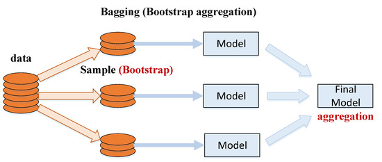
Figure 1.
Process flow of the bagging (bootstrap aggregation) algorithm.
Bagging has been used to solve classification problems in various fields. For instance, Lin [19] established an ensemble model to predict the credit rating of listed companies; the average misclassification rate for the bagging model was 24.9%, which was a significant improvement of 25.75% compared to the performance of a single classifier neural network model. Tang et al. [20] established a model to predict traffic congestion and achieved an overall prediction accuracy of up to 90.6% when the bagging algorithm was run for 10 iterations, demonstrating that bagging provided significantly better predictions than a single model. Furthermore, Hsieh [21] used patient discharge summaries to determine International Classification of Diseases (ICD) codes and adopted a bagging approach to enhance the accuracy of Bayesian classification; notably, a classification accuracy of up to 83.12% was achieved with bagging, which was 2% higher than that of the original Bayesian classification method. Mbogning and Broet [22] developed a bagging survival tree procedure using genomic data for variable selection and prediction with datasets containing non-susceptible patients; this procedure achieved satisfactory results with datasets containing the data of patients with early-stage breast carcinoma. Bagging can be considered a characteristic of random forests (RFs) in which the final prediction is obtained by averaging the predictions of individual trees. Kieu et al. [23] developed an ensemble learning framework that used binary voting (yes/no) to obtain the majority vote of classifiers for the prediction of customer booking behavior and demand using the observed data of a suburban on-demand transport service. The developed framework provided a better prediction accuracy than traditional supervised classification methods, such as logistic regression (LR), RF, SVM, and other ensemble techniques. Mosavi et al. [24] developed a novel prediction system to estimate groundwater potential more accurately for informed groundwater resource management to address the rapidly increasing demand for groundwater, which is a principal freshwater resource. The bagging models (i.e., RF and Bagged CART) performed better than the boosting models (i.e., AdaBoost and GamBoost). Importantly, the prediction results of the study may aid managers and policymakers in watershed and aquifer management to preserve and optimally exploit important freshwater resources.
Considering that the models developed in this study require algorithmic explainability and the ability to process imbalanced samples, we selected five algorithms for ensemble learning: LR (logistic regression algorithm), classification and regression trees (CART), C5.0 and naive Bayes (decision tree algorithms), and RF (ensemble learning algorithm). These machine learning classification algorithms are supervised learning methods that can make output predictions based on functions when given new data. Among the data mining methods commonly used in recent years, ensemble learning algorithms, which combine multiple machine learning classifiers, are the most widely applied in various fields. From the literature described above, it is apparent that bagging-based models provide better predictive performance than non-bagging-based models. Therefore, we adopted the bagging RF algorithm proposed by Mbogning and Broet [22] to enhance the predictive ability of our models. We also implemented a majority voting ensemble learning method based on LR and RF, as described by Kieu et al. [23], and RF and Bagged CART, as described by Mosavi et al. [24].
3. Materials and Methods
3.1. Data Sources and Tools
The main data sources of this study were data from border food inspections conducted in Taiwan, food inspection data, food product flow data, food product inspection and test data, business registration data, and food safety-related open databases around the world, including the gross domestic product (GDP), GDP growth rate, Global Food Security Index (GFSI), Corruption Perceptions Index (CPI), Human Development Index (HDI), Legal Rights Index (LRI), and Regional Political Risk Index (PRI) (Table 1), which provided a total of 125 different factors. Data analysis was performed using Tableau 2019.2, R 3.5.3, and Microsoft Excel 2010.

Table 1.
Type and sources of characteristic factors.
3.2. Study Process
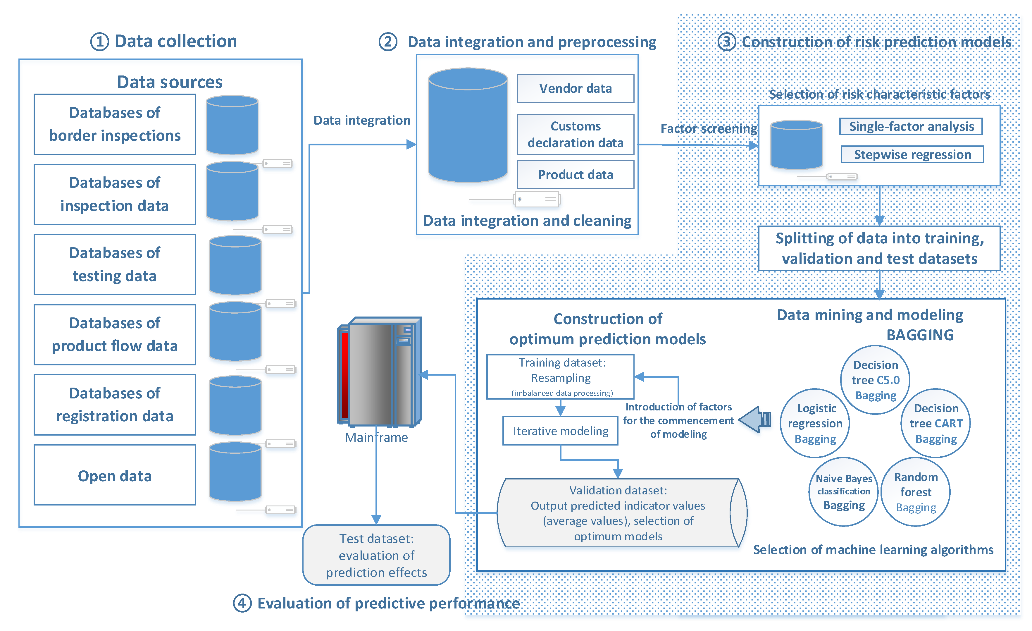
The top three product classes (named A, B, and C) with the highest non-conformity hit rates in the historical data of border inspections were selected as the scope for data modeling and predictions in the present study. Using data from border food inspections, risk prediction models were constructed using ensemble learning to serve as reference for the establishment of risk prediction models for random border inspections of imported food. The study process can be divided into four stages: data collection, data integration and preprocessing, construction of risk prediction models, and evaluation of predictive performance. Figure 2 shows a flowchart of the study process.
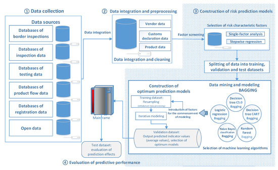
Figure 2.
Study process flowchart.
3.2.1. Data Collection
In the present study, product classes A, B, and C in border inspections were set as the targets of our analysis. In addition to using product-oriented data, such as data related to border inspections, products, manufacturers, customs brokers, and importers, we also included the inspection and test results of manufacturers and products and the open data of other countries in our analysis through factor connections as part of the main data sources for the construction of risk prediction models. A total of 125 factors were included in the analysis, as shown in Table 1.
3.2.2. Data Integration and Preprocessing
Missing values are often present in the data of many characteristic factors in various datasets. Data preprocessing is necessary as relationships may exist among the factors, but the arbitrary deletion of factor data may result in the partial loss of information and data, which affects the model prediction results. However, the retention of complete factor data may also lead to poorer predictive performance because of model overfitting. Considering the inability of most models to deal with missing values, we substituted the missing values with the average values in this study. The data integration and preprocessing stage of the study involved two main work processes: (1) Establishment of consistent linkage names for food products and vendors. The purpose of this process was to ensure the smooth execution of the subsequent database connection and analysis steps. Factors were sorted on the basis of individual border inspections and various data to establish consistent linkage names, which were used to connect the various databases to generate the datasets required for modeling. (2) Data cleaning for noise removal. Missing data were substituted to ensure the representativeness and accuracy of the data to be analyzed. The main purpose of this stage was to resolve difficulties in data identification because of a lack of standardized data formats, which rendered these data unusable. Examples of noise in the data included punctuation marks, special symbols, and missing or mismatched characters. Inconsistencies in product and vendor name formats in the data were also resolved by data cleaning to reduce the amount of noise in the data.
3.2.3. Construction of Risk Prediction Models
Risk Characteristic Factor Selection
The integrated and preprocessed data were subjected to a two-stage variable screening process in which risk characteristic factors were selected for inclusion in model construction. During the first stage, single-factor analysis was performed to identify factors that had statistically significant relationships with conformity or non-conformity during inspections and exhibited statistically significant differences. Different statistical tests were adopted depending on the variable type; categorical variables, such as customs district, year and month of border inspection, import and export methods, and country of manufacture, were analyzed using Fisher’s exact test, and continuous variables, such as GDP, duty-paid value in New Taiwan dollars, registered capital of vendor, and transportation time, were analyzed using the Wilcoxon rank-sum test. During the second stage, stepwise regression was performed to select risk factors with higher explanatory power for model simplification. As the purpose of this stage was to gather factors with significant influences from the previous stage for the efficient selection of optimum factor combinations, we adopted forward-backward stepwise regression for factor selection in the second stage. First, a single-factor LR was established, and F-values were determined for the corresponding regression coefficients (a larger F-value indicates that the factor has a higher explanatory power for the model). In the forward stepwise regression process, all factors that had not been included in the model were individually evaluated by calculating the F-values, and factors with the largest F-values were subsequently selected for inclusion in the model. The backward stepwise regression process involved the calculation of F-values for all factors that had already been included in the model, followed by deletion of variables with the smallest F-values. In the forward-backward stepwise regression method employed in the present study, which combined the features of the two aforementioned methods, forward and backward stepwise regressions were performed in alternation to achieve efficient determination of the optimum factor combinations. For variables with statistical significance (p < 0.05), stepwise regression was subsequently performed to serve as a basis for variable screening.
Splitting of Data into Training, Validation, and Test Datasets
To obtain optimum models, perform model validation, and evaluate model performance, the study data were split by year into the training (2011–2017), validation (2018), and test (2019) datasets prior to modeling (Figure 3). After the risk models were constructed, we divided the historical data used for modeling into test, training, and validation datasets, followed by oversampling to address data imbalance in the training dataset. The main purpose of resampling was to enhance the discriminatory ability of the model rather than to learn erroneous samples. If sampling is performed before data splitting, the resultant data of the test dataset will deviate from the original data. Consequently, noise in the data will be learned by the model, which will cause deviations in model predictions.
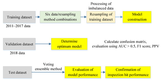
Figure 3.
Prediction model construction flowchart.
Data Mining and Modeling
Six data/resampling method combinations were established: the training dataset was classified by year into short-term (2016–2017) and long-term (2011–2017) data, blacklisted vendors were classified into inclusion or non-inclusion groups, and different resampling methods were used to process imbalanced data (scale-up and synthetic minority over-sampling technique (SMOTE)). Five data mining methods, namely, Bagging-C5.0, Bagging-CART, Bagging-BN, Bagging-RF, and Bagging-Logistic, were used for classifier construction. Iterative modeling was then performed for 10 iterations, and the average values were used for model construction. During model building with the training dataset, the characteristic factors to be included in the model were identified simultaneously.
Resampling for Training Dataset
Model prediction biases were likely because cases of product non-conformity only accounted for a small portion of the border inspection results. Therefore, oversampling was adopted in this study to achieve a conformity:non-conformity ratio close to 7:3. Two oversampling methods were utilized: scaling up the number of non-conformities and SMOTE. The latter approach involves the generation of new samples by interpolating between adjacent minority class samples to increase the proportion of non-conforming samples, thereby enhancing the model detection ability. In the present study, the effects of oversampling on model performance were evaluated using conformity:non-conformity ratios of 7:3, 6:4, 5:5, 4:6, and 3:7 achieved with SMOTE and 7:3 achieved with scaling. Our modeling results using the test dataset indicated that 7:3 was the optimum ratio.
Iterative Modeling
After resampling to obtain balanced data in the training dataset, iterative modeling was performed for 10 iterations to reduce misclassifications caused by single sampling errors. The results of each validation were saved, and the average values were ultimately calculated to serve as model selection criteria under different parameter conditions.
Selection of Optimum Model
In the present study, to select the optimum model and evaluate model performance, model effects were measured and validated using a confusion matrix and model predictive performance indicators. A confusion matrix was constructed using the entries defined in Table 2, and the required predictive performance indicators were calculated using the numbers of true positives (TP), false positives (FP), true negatives (TN), and false negatives (FN). Predictive performance indicators included accuracy (ACR), positive predictive value (PPV) (also known as precision), Recall, F1 score, and area under curve (AUC), which are described in detail below.
Table 2.
Definitions of entry types in the confusion matrix of this study.
- The accuracy rate (ACR) measures the overall discriminatory power of the model toward samples, i.e., the ability to classify conforming samples as conforming and non-conforming samples as non-conforming. However, an imbalance was present in the samples of the present study because of the smaller number of non-conformities in our data. Therefore, ACR may reflect a tendency toward the prediction of conformities because of the stronger discriminatory power toward conformity. To address this issue, greater emphasis was placed on Recall and PPV during the evaluation of model performance. ACR was calculated using Equation (1):ACR = (TP + TN) / (TP + TN + FP + FN)
- Recall or sensitivity is the proportion of samples correctly classified as non-conforming among all the samples that are actually non-conforming, as shown in Equation (2):Recall = TP / (FN + TP)
- Positive predictive value (PPV) or precision is the proportion of samples that are actually non-conforming among all the samples classified as non-conforming by the model, i.e., the non-conformity hit rate. PPV was calculated using Equation (3):PPV = TP / (TP + FP)
- F1 score, defined as the harmonic mean of Recall and PPV, is particularly important when working with imbalanced data. In the present study, model performance was estimated using the F1 score by assuming that the PPV and F1 thresholds were 0.5, i.e., equal weights were assigned. Larger F1 scores are indicative of higher TP values. The F1 score was calculated using Equation (4):F1 = 2(PPV × Recall) / (PPV + Recall) = 2TP / (2TP + FP + FN)
- Area under the receiver operating characteristics (ROC) curve (AUC) is a measure of the classification accuracy of the model; a larger AUC indicates higher accuracy. AUC = 1 denotes a perfect classifier, 0.5 < AUC < 1 indicates that the model is superior to random guessing, AUC = 0.5 indicates that the model is comparable to random guessing and does not possess classification ability, and AUC < 0.5 denotes a classifier inferior to random guessing.
After iterative modeling, the 2018 data in the validation dataset were used for prediction by the established models, and the optimum model was selected according to the values of predictive performance indicators used for model evaluation. In the present study, we used a confusion matrix to evaluate the classification prediction results and model predictive performance. The classification prediction results were first calculated, and models with AUC > 0.5 were then selected for comprehensive evaluation. As the present study was mainly focused on the non-conformity hit rate, PPV (i.e., the proportion of samples that are actually non-conforming among all the samples classified as non-conforming by the model) was used as the key indicator for model evaluation. Recall (sensitivity) was also used to evaluate the accuracy of the model in correctly classifying non-conforming samples. However, higher Recall values also indicate higher inspection rates. Therefore, an increase in PPV to achieve a balance between Recall and PPV within a tolerable range of inspection rates is crucial for the determination of predictive performance.
3.2.4. Evaluation of Predictive Performance
To determine the predictive performance of the model, model predictions were made using the 2019 data of the test dataset to simulate predictions when the model was implemented online. Similar to the process used to select the optimum prediction model, a confusion matrix was also used for the evaluation of predictive performance, with PPV and Recall as the evaluation indicators. Both the non-conformity hit rate and inspection rate were calculated and compared with the values of the previous year. To evaluate the overall model predictive performance, the presence or absence of significant changes in the non-conformity hit rate and inspection rate were determined using the chi-squared test.
4. Results
4.1. Processing Methods for Imbalanced Samples and Optimum Conformity: Non-Conformity Ratio
The scarcity of non-conformities in the present study made it necessary to adopt measures to increase the number of minority samples. Scaling up is conventionally used because of its simple working principle, which merely involves scaling up the data of minority classes to achieve the desired ratio. In the present study, scaling was performed to reach a conformity:non-conformity ratio of 7:3, a ratio adopted during modeling with the training dataset. Synthesized minority oversampling technique (SMOTE), another approach used to increase the number of minority samples, is commonly implemented in a number of ways: resampling of minority samples, sampling by certain distribution methods, or artificial synthesis of samples. In the present study, the minority class was oversampled by synthesizing new samples near the existing minority samples using the following procedure:
- Set a value for the required amount of oversampling (N), which represents the number of samples to be synthesized for each sample.
- Set a value for the number of nearest neighbors to be considered (K), determine the K nearest neighbors, and randomly select one sample from these K neighboring samples.
- Generate N samples using Equation (5):
A minority sample was first randomly selected, and its K nearest neighbors was identified (if K was set to 3, the 3 nearest neighbors were identified). From these neighboring samples, one was randomly selected for the synthesis of N new samples using Equation (5) (if N was set to 3, the randomly selected sample was used to generate 3 samples).
The modeling process consisted of two stages. In the first stage, the characteristic factors were identified, and in the second stage, imbalanced samples in the overall data were processed. We adopted the commonly used scaling up method and SMOTE to determine the most appropriate processing method for data imbalance and the optimum conformity:non-conformity ratio to be used for further experimentation. Five ratios (7:3, 6:4, 5:5, 4:6, and 3:7) were selected for 10 iterations of modeling using five types of algorithms combined with bagging. The average results of each model were used for majority voting ensemble learning to generate the classification results, and the predictive performance was evaluated by comparing PPV, Recall, and F1 score for the various imbalanced data processing methods and selected ratios.
Table 3 shows a comparison of the results obtained using different sampling ratios for minority samples when ensemble learning was performed on the training dataset comprising data from border inspections of food products belonging to classes A, B, and C. Because higher PPV and F1 scores indicate better predictive performance, it follows that a sampling ratio of 7:3 provided the best results for products of classes A, B, and C; the corresponding values of the performance measures were (1) class A: PPV = 25.08%, Recall = 65.25%, F1 score = 0.3624; (2) class B: PPV = 2.24%, Recall = 88.64%, F1 score = 0.0437; and (3) class C: PPV = 7.25%, Recall = 65.73%, F1 score = 0.1307.
Table 3.
Comparison of model predictive performances for different resampling methods and ratios adopted for imbalanced data processing.
When calculations were performed with the different methods and ratios adopted for processing imbalanced data, namely, “Scale-up 7:3,” “SMOTE 7:3,” “SMOTE 6:4,” “SMOTE 5:5,” “SMOTE 4:6,” “SMOTE 3:7,” and the methods and ratios were ranked in ascending order of the sum of the results, it was found that 7:3 was the optimum ratio. Considering that this ratio also provided the highest F1 scores in the three product classes, we adopted 7:3 as the parameter value for the conformity:non-conformity ratio for subsequent experimentation. Both scale-up and SMOTE were jointly used for modeling to determine the optimum model.
4.2. Optimum Number of Modeling Iterations
The timeliness of modeling is of great importance to the practical operation of the prediction model, as it directly affects the length of time required for first-line personnel to judge whether a food product is risky and whether it requires quality inspection. Although a larger number of iterations allows for more comprehensive considerations in the overall model, an excessive number of iterations also affects the time required for modeling operation, thereby reducing the predictive performance. In the present study, we found that the results obtained with 10 iterations were comparable to those obtained with 100 iterations, but the time required for 100 iterations was 3–8 times that of 10 iterations. To ensure that adequate iterations were used, the optimum number of modeling iterations was set to 10 for the five types of algorithms, and the values obtained from the iterations were averaged to serve as the final prediction results of each model.
4.3. Optimum Prediction Model
To establish the optimum risk prediction model, a total of six combinations of short-/long-term training data, inclusion/non-inclusion of blacklisted vendors, and different minority resampling methods were established to generate different characteristic factor screening results, as shown in Table 4. Modeling was then performed with each of the data/resampling method combinations using the five algorithms, namely, Bagging-Logistic, Bagging-CART, Bagging-C5.0, Bagging-NB (Bayesian classification), and Bagging-RF. Subsequently, the models were run with the validation dataset, and the prediction results of the five methods were further subjected to majority voting ensemble learning. A probability threshold value of 0.5 was set for the five types of algorithms, i.e., inspection was recommended when probability > 0.5 and not recommended when probability < 0.5. When a certain batch of customs declarations was classified as non-conforming by three or more of the five methods, the model recommended inspection, and the prediction results of ensemble learning were obtained.
Table 4.
Data/resampling method combinations for the risk prediction models.
Among the various data/resampling method combinations, the combinations of 2016–2017 data/non-inclusion of blacklisted vendors/SMOTE and 2016–2017 data/non-inclusion of blacklisted vendors/scale-up were not included for modeling, as there were fewer data on blacklisted vendors in the 2016–2017 dataset. Given that there were also few non-conforming batches during this interval, the importance of blacklisted vendors as a factor was further diminished. Therefore, these two data/resampling method combinations were eliminated because of their limited contribution to model prediction.
4.3.1. Optimum Data Combinations
The six data/resampling combinations mentioned above were used for ensemble learning, and modeling was subsequently performed after majority voting. The modeling results were validated using the validation dataset (2018 data) to determine the optimum data/resampling combinations (Table 5). For each food product class, the optimum combination was as follows:
Table 5.
Evaluation of various data/resampling method combinations.
- The optimum combination for class A was Scale-up/2011–2017 data/inclusion of blacklisted vendors, and the values of the predictive performance indicators were ACR = 86.6%, F1 score = 48.0%, PPV = 55.3%, and Recall = 42.4%.
- The optimum combination for class B was SMOTE/2011–2017 data/inclusion of blacklisted vendors, and the values of the predictive performance indicators were ACR = 93.9%, F1 score = 18.5%, PPV = 11.4%, and Recall = 48.0%.
- The optimum combination for class C was Scale-up/2011–2017 data/inclusion of blacklisted vendors, and the values of the predictive performance indicators were ACR = 94.4%, F1 score = 22.0%, PPV = 24.5%, and Recall = 19.9%.
Our results revealed that the optimum data/resampling method combinations differed among the different food product classes. Both scale-up and SMOTE served as optimum resampling methods in different optimum combinations, while the data interval and choice of inclusion/non-inclusion of blacklisted vendors in all optimum combinations were 2011–2017 and inclusion, respectively. These results indicate that the selection of different food classes leads to different optimum data/resampling method combinations. Therefore, “Scale-up/2011–2017 data/-inclusion of blacklisted vendors,” “SMOTE/2011–2017 data/inclusion of blacklisted vendors,” and “Scale-up/2011–2017 data/inclusion of blacklisted vendors” were separately used as the optimum combinations for product classes A, B, and C for subsequent construction of the prediction models.
The prediction results generated with the validation dataset were optimum when different data/resampling method combinations were used for product classes A, B, and C. In the present study, the prediction results were considered optimum when AUC > 50% and the values of the F1 score and PPV were as large as possible. A large F1 score indicates that optimum balance is achieved between PPV and Recall, which leads to optimum prediction results. Among the various data/resampling method combinations for the three product classes, both scale-up and SMOTE were the optimum resampling methods, whereas 2011–2017 or 2016–2017 data and inclusion of blacklisted vendors were the optimum choices for classes A and C.
4.3.2. Generation of Optimum Prediction Model
In the present study, ensemble learning was performed using six data/resampling method combinations with five bagging algorithms, namely, Bagging-CART, Bagging-Logistic, Bagging-NB, Bagging-C5.0, and Bagging-RF. Using the prediction results, the predictive performance indicators were calculated, and F1 score, PPV, Recall, and AUC were used to evaluate the prediction results to obtain the optimum data/resampling method combinations for the three border inspection product classes, which were “Scale-up/2011–2017 data/inclusion of blacklisted vendors” for class A, “SMOTE/2011–2017 data/inclusion of blacklisted vendors” for class B, and “Scale-up/2011–2017 data/inclusion of blacklisted vendors” for class C.
To generate the optimum prediction model, the optimum data/resampling method combinations were first adopted for machine learning using five single bagging-type algorithms and ensemble learning, and the prediction results of the various algorithms were compared. The model with the highest values for F1 score, PPV, and Recall and with AUC > 50% (i.e., the predictive performance of the model was better than that of random guessing) was considered the optimum model.
Table 6, Table 7 and Table 8 show the predictive performances of the various models obtained with the validation data for food product classes A, B, and C. For class A products, the data/resampling method combination used was “Scale-up/2011–2017 data/inclusion of blacklisted vendors.” The predictive performance indicator values obtained using ensemble learning (No. A4) were F1 score = 48.0%, PPV = 55.3%, and AUC = 78.3% (>50%). Similar values were obtained with the Bagging-Logistic algorithm (F1 score = 48.0%, PPV = 53.8%, and AUC = 70.3%). The Bagging-CART algorithm provided the best predictive performance, with an F1 score of 53.9%, PPV of 52.4%, and AUC of 77.5%. For class B products, the data/resampling method combination used was “SMOTE/2011–2017 data/inclusion of blacklisted vendors.” The predictive performance indicator values obtained using ensemble learning (No. B2) were F1 score = 18.5%, PPV = 11.4%, and AUC = 81.1% (>50%). Bagging-Logistic achieved the highest F1 score, with predictive performance indicator values of F1 score = 18.6%, PPV = 11.5%, and AUC = 78.0%. For class C products, the data/resampling method combination used was “Scale-up/2011–2017 data/inclusion of blacklisted vendors.” The predictive performance indicator values obtained using ensemble learning (No. C2) were F1 score = 22.0%, PPV = 24.5%, and AUC = 67.2% (>50%). Bagging-CART achieved the highest F1 score, with predictive performance indicator values of F1 score = 23.6%, PPV = 16.9%, and AUC = 66.1%. The results described above indicated that ensemble learning provided relatively stable predictive performance compared with other algorithms. Although the predictive performance of ensemble learning was not the best algorithm, it was also not the worst and was superior to random guessing (AUC > 50%). Therefore, ensemble learning was selected as the optimum prediction model. The predictive performance of the model was subsequently determined through model prediction using the test dataset (2019 data).
Table 6.
Comparison of prediction models for class A products.
Table 7.
Comparison of prediction models for class B products.
Table 8.
Comparison of prediction models for class C products.
4.3.3. Model predictive performance
The model obtained using ensemble learning was set as the optimum prediction model and used for the simulation of online model implementation using the test dataset (2019 data). Subsequently, the risk predictive performance of the model was evaluated by selecting inspection batches with risk threshold values of 0.5 and above for the various algorithms. Considering that the historical 2019 inspection data were obtained by random sampling, i.e., inspection results were only available for certain inspection batches, samples that were randomly selected for inspection were screened to evaluate model performance. Table 9 and Table 10 show the results of model prediction.
Table 9.
Model predictive performance indicators for model prediction on the test dataset for product classes A, B, and C.
Table 10.
Risk prediction performance for product classes A, B, and C.
In 2019, a total of 3643 batches of class A products were declared, of which 770 batches were randomly inspected and the inspection results were available (note: this is not the total number of batches declared in the entire year). The data of these 770 declared batches with available inspection results were used as the test dataset for model prediction. The model prediction results were as follows: recommended number of batches to be inspected: 40, recommended inspection rate: 5.19%, hit rate: 55.00%, and number of model hits: 22. The actual inspection rate, hit rate, and number of non-conforming batches were 18.64%, 15.76%, and 107, respectively. Therefore, the hit rate predicted by the model was approximately 3.5 times the hit rate of the existing random inspection method.
A total of 23,011 batches of class B products were declared in 2019, of which 1975 batches were randomly inspected and the inspection results were available (note: this is not the total number of batches declared in the entire year). The data of these 1975 declared batches with available inspection results were used as the test dataset for model prediction. The model prediction results were as follows: recommended number of batches to be inspected: 77, recommended inspection rate: 3.90%, hit rate: 12.99%, and number of model hits: 10. The actual inspection rate, hit rate, and number of non-conforming batches were 7.51%, 1.51%, and 26, respectively. Therefore, the hit rate predicted by the model was approximately 8.6 times the hit rate of the existing random inspection method.
A total of 37,387 batches of class C products were declared in 2019, of which 5059 batches were randomly inspected and the inspection results were available (note: this is not the total number of batches declared in the entire year). The data of these 5059 declared batches with available inspection results were used as the test dataset for model prediction. The model prediction results were as follows: recommended number of batches to be inspected: 126, recommended inspection rate: 2.49%, hit rate: 25.40%, and number of model hits: 32. The actual inspection rate, hit rate, and number of non-conforming batches were 12.31%, 2.72%, and 26, respectively. Therefore, the hit rate predicted by the model was approximately 9.3 times the hit rate of the existing random inspection method.
In summary, the use of ensemble learning as the optimum model for product classes A, B, and C led to higher model-predicted hit rates compared with random inspection for all three product classes.
5. Discussion
5.1. Comparison of Single Algorithms with Ensemble Learning
On the basis of the prediction model construction methods reported in the literature, five commonly used machine learning algorithms were separately combined with bagging to obtain the algorithms Bagging-Logistic, Bagging-CART, Bagging-C5.0, Bagging-NB, and Bagging-RF. These five algorithms were subsequently used with ensemble learning to construct model classifiers, and the predictive performance of single algorithms and the ensemble learning model was evaluated. The predictive performance indicators used in this study were AUC, F1 score, PPV, and Recall. PPV refers to the proportion of samples that are actually non-conforming among all the samples classified as non-conforming by the model. Recall, also known as the true positive rate (TPR), refers to the proportion of samples correctly classified as non-conforming among all the samples that are actually non-conforming. The ROC curve is a plot of Recall (TPR) against the false positive rate (FPR) at various threshold levels, and a larger area under the ROC curve (AUC) signifies better predictive performance. An AUC value between 0.5 and 1 indicates that the model is better than random guessing and possesses prediction value. F1 score is defined as the harmonic mean of Recall and PPV. A high F1 score indicates that the values of Recall and PPV are comparable, as an extremely small value of either indicator generally leads to a considerably lower F1 score.
Table 11 shows the values of the various predictive performance indicators for class A products. Among the various algorithms, ensemble learning achieved the highest AUC value, demonstrating its superiority over any single algorithm. Therefore, there is a higher probability that a sample predicted as non-conforming by the ensemble learning model is actually non-conforming, i.e., a lower false-positive risk. The AUC values also indicated that all single algorithms and the ensemble learning method provided better predictive performance than random inspection. In comparing the PPV of the various algorithms, ensemble learning (PPV = 55.0%) was superior to the single algorithms (PPV = 25.0–52.6%). Therefore, ensemble learning provided the highest number of hits for truly non-conforming batches among the batches predicted as non-conforming. The PPV of Bagging-RF was close to that of ensemble learning (52.6 vs. 55.0%), indicating high performance compared with other single algorithms. Ensemble learning achieved a Recall value of 19%, which was close to the mid-point of the range 8.6–34.5% for the various algorithms. According to the overall performance, ensemble learning is the optimum prediction model for class A products.
Table 11.
Predictive performance of various algorithms on the test dataset for class A products.
Table 12 shows the values of the various predictive performance indicators for class B products. The AUC of the various algorithms was within the range 58.9–78.6%. In particular, the AUC values of ensemble learning and Bagging-RF were almost identical at 78.4% and 78.6%, respectively. Therefore, both algorithms had similar abilities in predicting truly non-conforming batches, i.e., the possibility of false positives was relatively low with both algorithms. All AUCs > 50%, indicating that all single algorithms and ensemble learning provided better predictive performance than random inspection. However, the AUC of Bagging-Logistic was only 58.9%, making it the poorest performing algorithm.
Table 12.
Predictive performance of various algorithms on the test dataset for class B products.
The PPVs of the various algorithms were within the range 7.4–13.7%; the PPV of Bagging-CART was the highest at 13.7%, and that of ensemble learning was close to the median PPV of the five single algorithms. This is consistent with the view held by Kieu et al. [23] that ensemble learning may not provide the best prediction results but avoids the selection of the worst classifier, which leads to greater stability in prediction. Although the PPV of ensemble learning was not higher than those of all the single algorithms, all the PPV values did not differ significantly. Therefore, the number of batches correctly predicted as non-conforming was similar among the algorithms. The Recall values were within the range 31.4–57.1%, and the value (40%) of ensemble learning was close to the median value. Considering the need to maintain prediction stability, ensemble learning was also selected as the optimum model for class B products.
Table 13 shows the values of the various predictive performance indicators for class C products. The AUC of the various algorithms were within the range 57.1–75.3%. In particular, the AUC values of ensemble learning and Bagging-RF were similar at 72.5% and 75.3%, respectively. Therefore, both algorithms had comparable abilities in identifying true positives and false positives, which was also reflected in the PPVs. All AUCs > 50%, indicating that all single algorithms and ensemble learning provided better predictive performance than random inspection. Despite achieving a high AUC, Bagging-RF had a low F1 score of 9.8%, indicating a poorer balance between PPV and Recall. By contrast, ensemble learning and Bagging-CART achieved better F1 scores of 23.0% and 28.6%, respectively.
Table 13.
Predictive performance of various algorithms on the test dataset for class C products.
The PPVs of all the algorithms were within the range 6.2–29.0%, and the PPV of ensemble learning was 25.4%. Although Bagging-RF had the highest PPV of 29.0%, its F1 score was significantly lower than those of most other algorithms, while ensemble learning exhibited relatively stable performance. The Recall values were in the range 5.9–46.1%, and the Recall value (21.1%) of ensemble learning was close to the median value. Considering the need to maintain prediction stability, ensemble learning was also selected as the optimum model for class C products.
5.2. Evaluation of Model Performance after Online Implementation
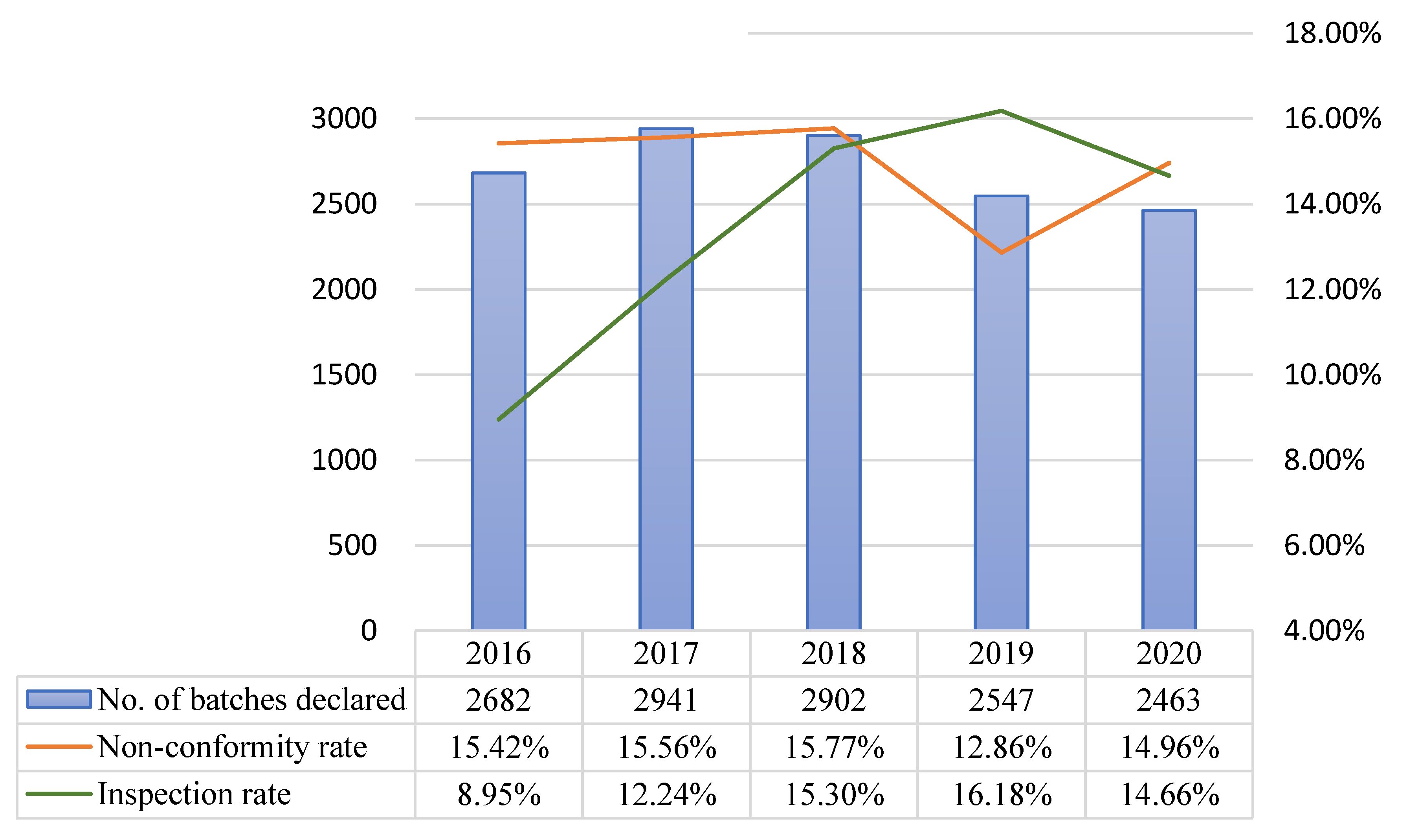
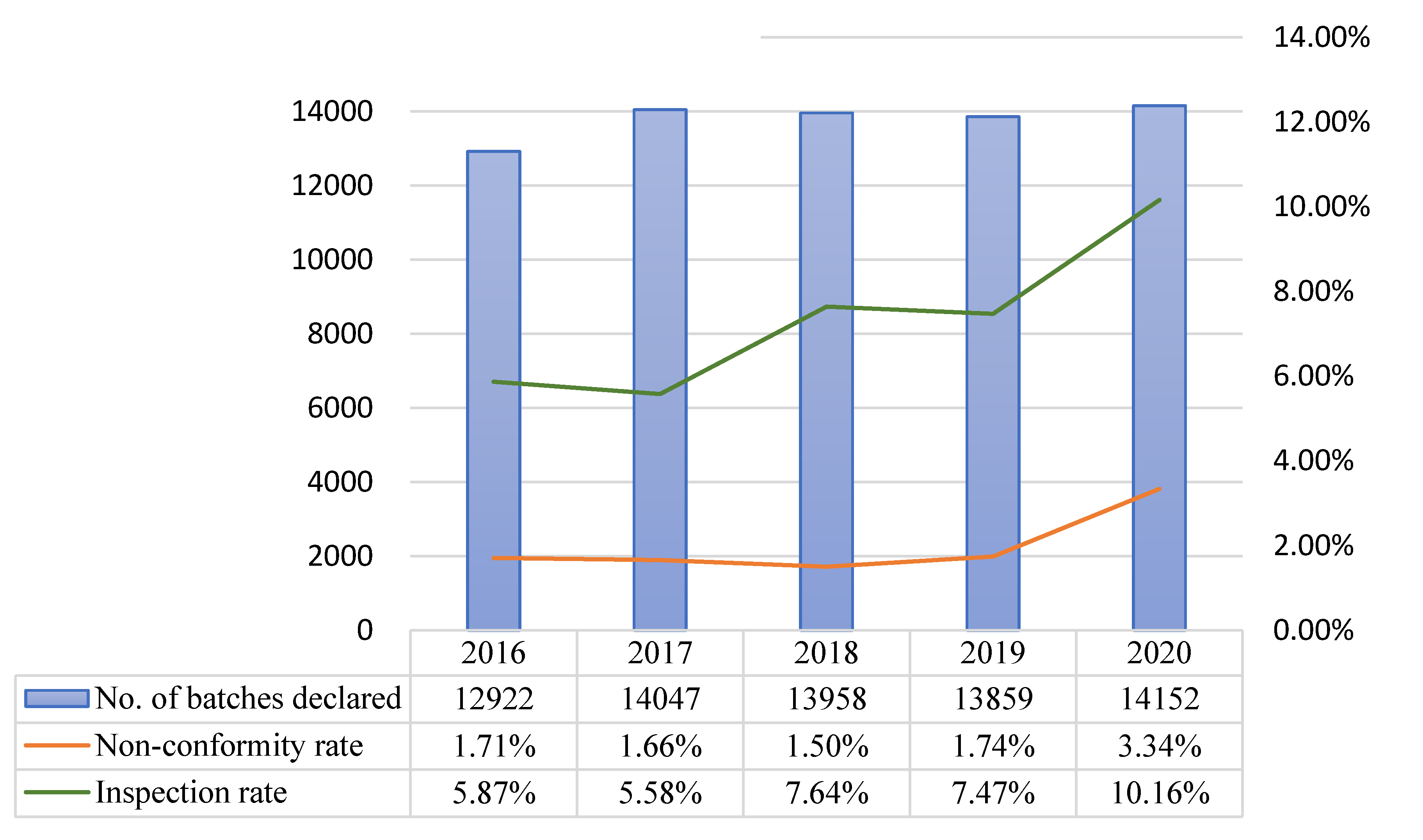
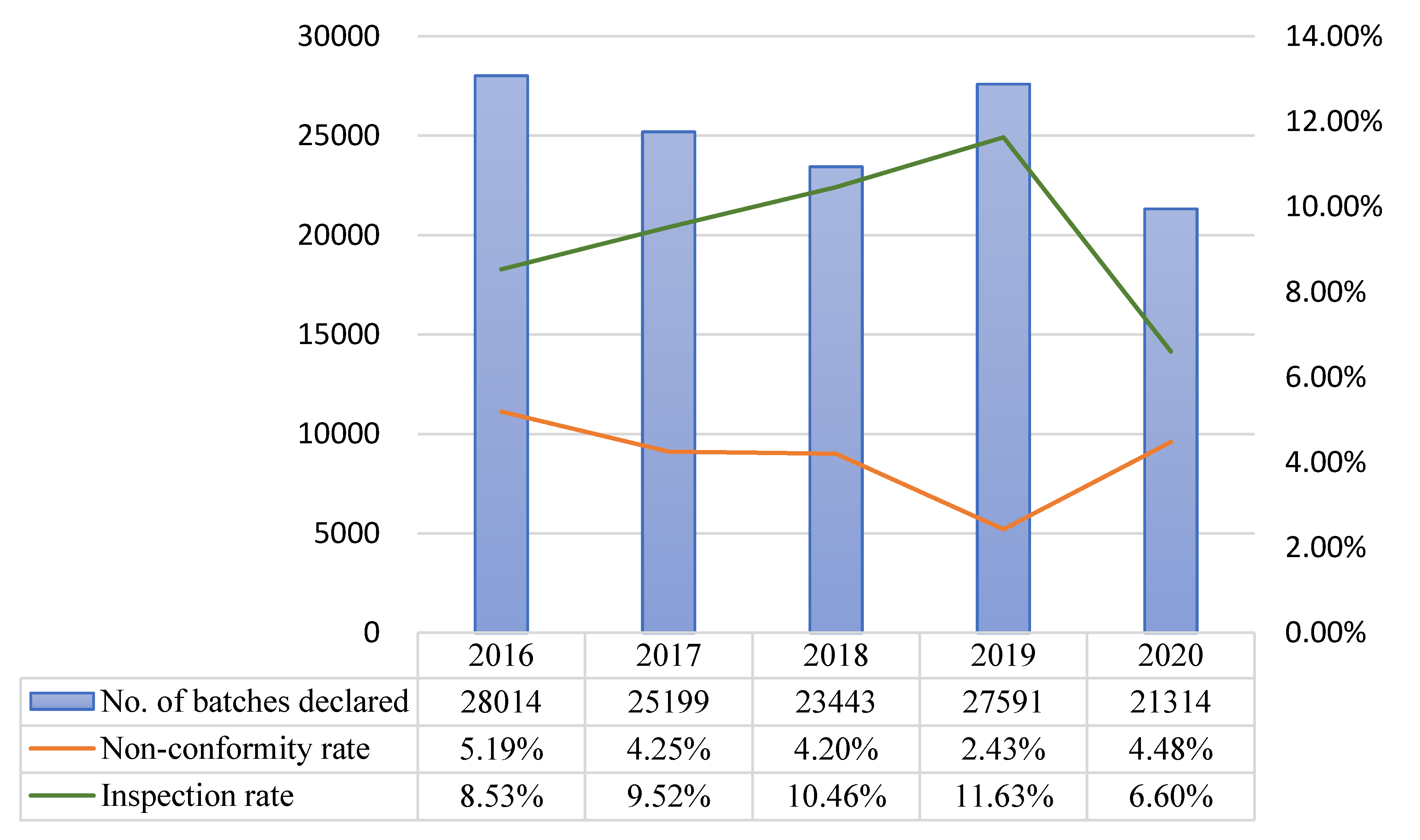
The models developed in this study were implemented online in 2020, and the model predictive performance for class A, B, and C products from the start of implementation to November 30 2020 were compared with the data of comparable periods (non-consecutive days) in previous years. In 2020, the number of non-conforming batches and non-conformity hit rate were respectively 54 and 14.96% for class A, 48 and 3.34% for class B, and 64 and 4.48% for class C. During the comparable period in 2019, the corresponding values were 53 and 12.86% for class A, 18 and 1.74% for class B, and 78 and 2.43% for class C. For both classes A and B, the number of non-conforming batches and non-conformity hit rate were higher in 2020 than in 2019 (Table 14 and Figure 4, Figure 5 and Figure 6).
Table 14.
Prediction results of risk prediction models for product classes A, B, and C after online implementation.
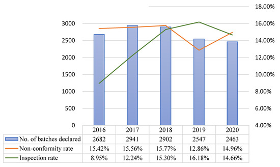
Figure 4.
Comparison of prediction results across years (comparable periods) for class A after model implementation.
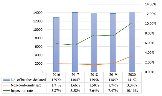
Figure 5.
Comparison of prediction results across years (comparable periods) for class B after model implementation.
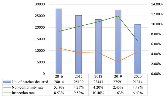
Figure 6.
Comparison of prediction results across years (comparable periods) for class C after model implementation.
After model implementation and operation, the inspection rate for class A decreased from 16.18% in 2019 to 14.66% in 2020, but the non-conformity hit rate increased from 12.86% in 2019 to 14.96% in 2020. Although the chi-squared test did not indicate the presence of statistically significant differences, the total number of inspected batches decreased, while the number of non-conforming batches remained approximately the same (53 in 2019 and 54 in 2020). For class B, the inspection rate increased from 7.47% in 2019 to 10.16% in 2020, and the non-conformity hit rate increased from 1.74% in 2019 to 3.34% in 2020. The results of the chi-squared test showed that the increases in inspection rate (p = 0.001 ***) and non-conformity hit rate (p = 0.021 *) were both statistically significant. Even though the inspection rate increased, the total number of non-conforming batches in 2020 was more than double that of the previous year. For class C, the inspection rate decreased from 11.63% in 2019 to 6.68% in 2020, and the non-conformity hit rate increased from 2.43% in 2019 to 4.48% in 2020. The results of the chi-squared test indicated that the decrease in inspection rate (p = 0.001 ***) and increase in non-conformity hit rate (p = 0.001 ***) were both statistically significant (Table 15).
Table 15.
Evaluation of predictive performance for product classes A, B, and C after online implementation of risk prediction models.
The results described above indicate that the prediction models established for food product classes A, B, and C effectively increase the hit rate of non-conforming batches, which contributes to risk prediction and prevention in border food inspections.
5.3. Learning Feedback Mechanisms
The ensemble learning method used in this study was implemented through majority decision using five machine-learning algorithms. The greatest limitation of this method is that the number of unqualified articles must be used as the learning goal to carry out prediction. The historical data of border food sampling inspection shows that not all food categories have unqualified cases; thus, it is impossible to perform machine learning through training, which is the main limitation of this study. Therefore, by merging the data of similar food categories, we have accumulated a small number of unqualified features for learning, and have arranged 1–3% random sampling in addition to the sampling method suggested by the ensemble learning method to avoid overfitting results. In this manner, the problem of too few unqualified articles can be solved and a robust model can be achieved.
In the present study, SMOTE was used for resampling to resolve the issue of data imbalance. Although SMOTE was established on the basis of data science, it involves sample synthesis using a small number of samples, which potentially introduces overfitting. Nonetheless, oversampling is still commonly adopted in practice to avoid choosing a model that lacks discriminatory power. In addition, sample synthesis by SMOTE is performed in a linear fashion, which does not alter the original state of the numerical data. This makes linear interpolation a reasonable method for sample synthesis. However, linear interpolation may introduce noise if the available data are not distributed in Euclidean space. Therefore, it is necessary to observe the data before applying the methods described in this study. To this end, we randomly inspected 1–3% of food products from various classes to observe the number of at-risk batches that may have been missed by model prediction. This provides feedback to the models for relearning and remodeling.
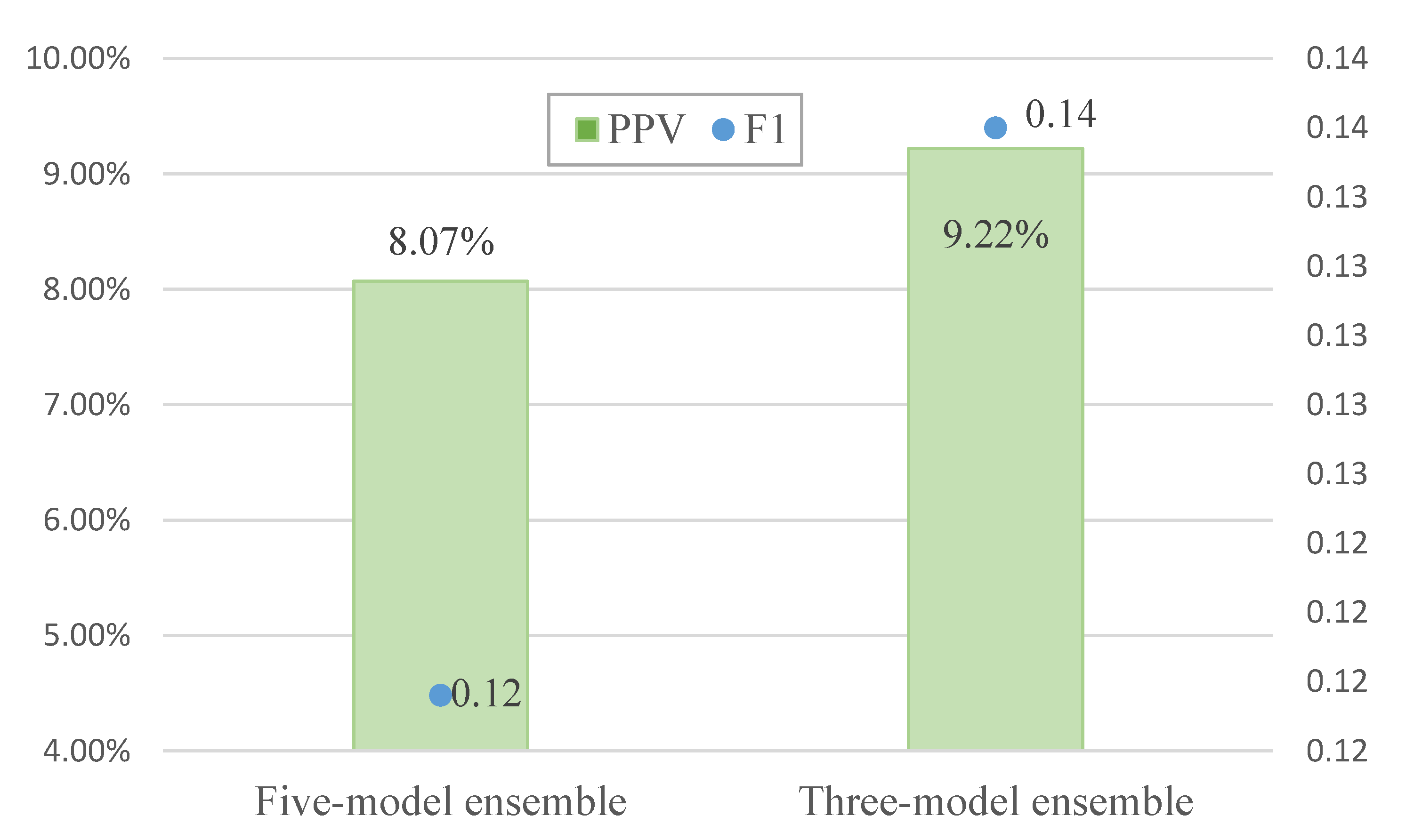
In the present study, the data of class A products were used in the five models established by machine learning algorithms, and model predictions were obtained for each batch of declared products. The decision to inspect each batch of products was then made on the basis of majority voting, i.e., inspection was performed if it was recommended by more than half of the models (three or more out of five). Therefore, the poorer performing models among the five models affected the overall predictive performance. When ensemble learning was carried out with the five models, the non-conformity hit rate (PPV or precision) was 8.07% and the F1 score was 0.12 (Figure 7). When the poorer performing logistic regression and naive Bayes classification models were removed and ensemble learning was performed using the remaining three models, the resulting non-conformity hit rate and F1 score were respectively 9.22% and 0.14, which were better than that of ensemble learning with five models (Figure 8). Therefore, selection mechanisms may be adopted in the design of inspection prediction methods after modeling to include the most appropriate algorithms in ensemble learning while maintaining the objectivity and accuracy of majority voting.
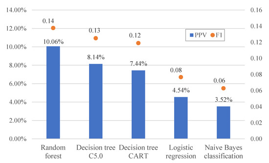
Figure 7.
Comparison of prediction results of the five models.

Figure 8.
Comparison of predictive performance before and after ensemble pruning.
6. Conclusions
The global COVID-19 pandemic in 2020 has greatly impacted the production, manufacture, importation, and exportation of raw food materials and food products in badly affected countries. In the present study, we used historical customs declaration data for food products imported into Taiwan to construct risk prediction models and evaluated the predictive performance of the models. The results indicated that the models significantly increased the hit rate of non-conforming batches among the declared batches and significantly decreased the inspection rate compared with random inspection. These findings may potentially serve as a valuable reference for the improvement of existing random inspection methods for imported food products. The results of this study are currently implemented in the border food quality sampling operation in Taiwan. Through this operation mode, the unqualified rate can be effectively reduced, the number of samples inspected can be reduced, and manpower and material costs can be saved.
In the present study, risk prediction models for border food inspection were constructed by performing ensemble learning with five different machine learning methods combined with bagging: Bagging-Logistic, Bagging-CART, Bagging-C5.0, Bagging-RF, and Bagging-NB. In addition to reviewing the relevance of the important characteristic factors on a regular basis, we also recommend continuous exploration of other critical characteristic factors for future modeling to further enhance predictive performance for non-conforming batches of imported food products. Compared with random inspection, the hit rate of non-conforming products and batch inspection rate are effectively increased using ensemble learning to perform predictions, which greatly reduces inspection costs and provides considerable benefits to food safety management. Therefore, if the ensemble learning models developed in this study can be progressively applied to predictions for all imported products, an automatic modeling and risk prediction system can be established for real-time feedback of daily declaration, inspection, and test results to the models. This will potentially aid in the continuous updating of risk prediction models to further improve the predicted hit rate of at-risk products by the models.
Author Contributions
Conceptualization, L.-Y.W. and S.-S.W.; methodology, L.-Y.W. and S.-S.W.; software, L.-Y.W.; validation, L.-Y.W. and S.-S.W.; formal analysis, L.-Y.W.; investigation, L.-Y.W.; resources, L.-Y.W.; data curation, L.-Y.W.; writing—original draft preparation, L.-Y.W.; writing—review and editing, S.-S.W.; visualization, L.-Y.W.; supervision, L.-Y.W. and S.-S.W.; project administration, L.-Y.W. and S.-S.W.; funding acquisition, no external funding, L.-Y.W. and S.-S.W. All authors have read and agreed to the published version of the manuscript.
Funding
This research received no external funding.
Institutional Review Board Statement
Not applicable.
Informed Consent Statement
Not applicable.
Acknowledgments
We would like to express our gratitude to the Food and Drug Administration of the Ministry of Health and Welfare of Taiwan for approving the execution of this study on 27 January 2021 (approval document No.: 1101190041).
Conflicts of Interest
The authors declare no conflict of interest.
References
- Bouzembrak, Y.; Marvin, H.J.P. Prediction of Food Fraud Type Using Data from Rapid Alert System for Food and Feed (RASFF) and Bayesian Network Modelling. Food Control 2016, 61, 180–187. [Google Scholar] [CrossRef]
- Marvin, H.J.P.; Janssen, E.M.; Bouzembrak, Y.; Hendriksen, P.J.M.; Staats, M. Big Data in Food Safety: An Overview. Crit. Rev. Food Sci. Nutr. 2017, 57, 2286–2295. [Google Scholar] [CrossRef] [PubMed] [Green Version]
- United States Government Accountability Office. Imported Food Safety: FDA’s Targeting Tool has Enhanced Screening, But Further Improvements are Possible; GAO: Washington, DC, USA, May 2016. Available online: https://www.gao.gov/products/gao-16-399 (accessed on 1 November 2021).
- Wolpert, D.H. The Supervised Learning No-free-lunch Theorems. In Soft Computing and Industry: Recent Application; Roy, R., Koppen, M., Ovaska, S., Furuhashi, T., Hoffmann, F., Eds.; Springer: London, UK, 2002; pp. 25–42. [Google Scholar]
- Pagano, C.; Granger, E.; Sabourin, R.; Gorodnichy, D.O. Detector Ensembles for Face Recognition in Video Surveillance. In Proceedings of the International Joint Conference on Neural Networks (IJCNN), Brisbane, Australia, 10–15 June 2012; pp. 1–8. [Google Scholar] [CrossRef] [Green Version]
- Pintelas, P.; Livieris, I.E. Special Issue on Ensemble Learning and Applications. Algorithms 2020, 13, 140. [Google Scholar] [CrossRef]
- Dasarathy, B.V.; Sheela, B.V.A. Composite Classifier System Design: Concepts and methodology. Proc. IEEE Inst. Electr. Electron. Eng. 1979, 67, 708–713. [Google Scholar] [CrossRef]
- Hansen, L.K.; Salamon, P. Neural network ensembles. IEEE Trans. Pattern Anal. Mach. Intell. 1990, 12, 993–1001. [Google Scholar] [CrossRef] [Green Version]
- Polikar, R. Ensemble Based Systems in Decision Making. IEEE Circuits Syst. Mag. 2006, 6, 21–45. [Google Scholar] [CrossRef]
- Suganyadevi, K.; Malmurugan, N.; Sivakumar, R. OF-SMED: An Optimal Foreground Detection Method in Surveillance System for Traffic Monitoring. In Proceedings of the International Conference on Cyber Security, Cyber Warfare and Digital Forensic, CyberSec, Kuala Lumpur, Malaysia, 26–28 June 2012; pp. 12–17. [Google Scholar] [CrossRef]
- Wang, R.; Bunyak, F.; Seetharaman, G.; Palaniappan, K. Static and Moving Object Detection Using Flux Tensor with Split Gaussian Models. In Proceeding of the IEEE Conference on Computer Vision and Pattern Recognition (CVPR) Workshops, Columbus, OH, USA, 23–28 June 2014; pp. 414–418. [Google Scholar] [CrossRef]
- Wang, T.; Sonoussi, H. Detection of Abnormal Visual Events via Global Optical Flow Orientation Histogram. IEEE Trans. Inf. Forensics Secur. 2014, 9, 998. [Google Scholar] [CrossRef]
- Tsai, C.J. New feature selection and voting scheme to improve classification accuracy. Soft Comput. 2019, 23, 12017–12030. [Google Scholar] [CrossRef]
- Cao, P.; Zhao, D.; Zaiane, O. Hybrid probabilistic sampling with random subspace for imbalanced data learning. Intell. Data Anal. 2014, 18, 1089–1108. [Google Scholar] [CrossRef] [Green Version]
- Feng, L.; Zhang, Z.; Ma, Y.; Du, Q.; Williams, P.; Drewry, J.; Luck, B. Alfalfa Yield Prediction Using UAV-Based Hyperspectral Imagery and Ensemble Learning. Remote Sens. 2020, 12, 2028. [Google Scholar] [CrossRef]
- Parastar, H.; van Kollenburg, G.; Weesepoel, Y.; van den Doel, A.; Buydens, L.; Jansen, J. Integration of Handheld NIR and Machine Learning to “Measure & Monitor” Chicken Meat Authenticity. Food Control 2020, 112, 1–11. [Google Scholar] [CrossRef]
- Neto, H.A.; Tavares, W.L.F.; Ribeiro, D.C.S.Z.; Alves, R.C.O.; Fonseca, L.M.; Campos, S.V.A. On the Utilization of Deep and Ensemble Learning to Detect Milk Adulteration. BioData Min. 2019, 12, 1–13. [Google Scholar] [CrossRef]
- Breiman, L. Bagging Predictors. In Technical Report No. 421; University of California: Oakland, CA, USA, September 1994; Available online: http://www.cs.utsa.edu/~bylander/cs6243/breiman96bagging.pdf (accessed on 10 November 2020).
- Lin, M.K. Visitant: A Structured Agent-Based Peer-to-Peer System. Master’s Thesis, Graduate Institute of Information Management, National Taiwan University, Taipei, Taiwan, 2004. [Google Scholar]
- Tang, Z.K.; Zheng, J.S.; Wang, W.Z. The Phase Sequence-changeable Control based on Fuzzy Neural Network of Isolated Intersection. J. Zhejiang Vocat. Tech. Inst. Transp. 2014, 7, 29–32. [Google Scholar]
- Hsieh, Y.S. Using Discharge Summary to Determine the International Classification of Diseases-9th Revision-Clinical Modification. Master’s Thesis, Graduate School of Information Management, National Yunlin University of Science and Technology, Yunlin, Taiwan, 2007. [Google Scholar]
- Mbogning, C.; Broet, P. Bagging Survival Tree Procedure for Variable Selection and Prediction in the Presence of Nonsusceptible Patients. BMC Bioinform. 2016, 17, 230. [Google Scholar] [CrossRef] [PubMed] [Green Version]
- Kieu, L.M.; Ou, Y.; Truong, L.T.; Cai, C. A Class-specific Soft Voting Framework for Customer Booking Prediction in On-demand Transport. Transp. Res. Part C Emerg. Technol. 2020, 114, 377–390. [Google Scholar] [CrossRef]
- Mosavi, A.; Hosseini, F.S.; Choubin, B.; Goodarzi, M.; Dineva, A.A.; Sardooi, E.R. Ensemble Boosting and Bagging Based Machine Learning Models for Groundwater Potential Prediction. Water Resour. Manag. 2021, 35, 23–37. [Google Scholar] [CrossRef]


Publisher’s Note: MDPI stays neutral with regard to jurisdictional claims in published maps and institutional affiliations. |
© 2021 by the authors. Licensee MDPI, Basel, Switzerland. This article is an open access article distributed under the terms and conditions of the Creative Commons Attribution (CC BY) license (https://creativecommons.org/licenses/by/4.0/).