Article

Location-Routing Optimization with Renting Social Vehicles in a Two-Stage E-Waste Recycling Network

1
Glorious Sun School of Business and Management, Donghua University, Shanghai 200051, China
2
School of Economics and Management, Tongji University, Shanghai 200092, China
*
Author to whom correspondence should be addressed.
Sustainability 2021, 13(21), 11879; https://doi.org/10.3390/su132111879
Submission received: 31 August 2021 / Revised: 13 October 2021 / Accepted: 22 October 2021 / Published: 27 October 2021

Abstract

:
E-waste recycling has been a hot topic in recent years. The low efficiency and high-operation cost of recycling make it more important to build perfect e-waste recycling networks. To hedge against the limitation of vehicle resources being often neglected in existing research, we propose a mixed integer linear programming model of e-waste recycling by renting idle social vehicles. In the model, both decisions made on the location selection of recycling sites and vehicle routings satisfying all of the demand nodes over the network within time windows are required to minimize the total operating cost. An improved genetic algorithm and heuristic algorithm are designed to solve the model, and numerical experiments are produced to demonstrate the effectiveness of the proposed model and algorithms.

1. Introduction

With the development of sharing economies and the advent of the “Internet +” wave, enterprises are constantly innovating new forms to figure out traditional pain points of various industries. Sharing economies can create social value and can improve the lives of people all over the world.
The shortened electrical and electronic product life-cycles, along with the rapid technological innovation and increased need of automated production, have made e-waste one of the fastest-growing waste streams. The recycling of e-waste is related to environment and resources. On one hand, e-waste is called urban minerals because of a large amount of high-value metals such as gold and copper [1]. On the other hand, it contains harmful substances that affect human health and damage ecological environment. How to recycle e-waste in a better way has always been a problem perplexing the industries and the markets.
There are three fundamental weaknesses of current e-waste recycling. First, the distances between demand nodes and recycling sites so far make it such that users with recycling demands are unwilling to discard e-waste to recycling sites by themselves. Second, if recycling sites arrange vehicles to pick up e-waste door to door, it is unlikely that vehicles can arrive at all of the demand nodes within their respective service time windows. Third, in the recycling sites, there are a limited number of owned vehicles that may not be able to satisfy recycling demands in time. On the other hand, it is uneconomic to equip more vehicles to satisfy peak demands.
In China, sharing models such as car sharing and bicycle sharing are prevalent. In metropolitan areas, there is a considerable degree of inefficiency in transporting trucks due to traffic congestion, etc., and small and medium-sized trucks that transport in urban areas, which are usually empty on the return trip. There are already companies in the business of leasing trucks at hourly rates. Thompson et al. [2] investigated the potential of shared networks for general freight transportation in urban areas in Melbourne to reduce congestion and to lower transportation costs, and the results show that sharing freight makes it possible to reduce transportation costs significantly.
This study makes decisions on the selection of recycling sites for constructing efficient e-waste recycling network, the selection of outsourcing demands to be satisfied by social vehicles, and vehicle routing solutions for the remaining demands, aiming to minimize the sum of the total rental cost and the total transportation cost in the recycling network. With the assumption of customer perferred time windows of service, selecting outsourcing demands has a great impact on the routing scheduling for the remaining demands to be completed by owned vehicles. The two choices of completing recycling demands, i.e., using social or owned vehicles, makes the problem decision more complicated. A full solution consists of deciding the locations of recycling sites, the selection of outsourcing demands, and making a vehicle routings schedule for the remaining demands in the e-waste recycling network. Note that selecting social vehicles causes some amount of renting fee. To minimize the total rental cost and the total transportation cost, the selection of which and how many demands to be served by social vehicles are closely related to the total capacity of vehicles and the preferred service time windows of customer demands.
The main contributions of this work are as follows:
  • Under the background of sharing economy, we introduce the application of social vehicles with rental cost into the classical integrated recycling cite location and vehicle routing problem in an e-waste recycling network. There are two stages of e-waste collection, where in the first stage, e-waste recycling demands are processed by either self-delivery or door-to-door pickup and, in the second stage, the collected e-wastes are delivered to the unique processing centre.
  • An MILP model is established, in which it is assumed that different recycling sites are equipped with an unequal number of vehicles, and each vehicle shall depart from and return to its respective recycling site in the first collection stage.
  • An improved genetic algorithm and a two-stage cyclic optimization-based heuristic algorithm are developed to solve the considered problem.
The rest of this paper is organized as follows. Section 2 reviews the relevant papers in the literature. In Section 3, the problem is stated and formulated. Next, a genetic and a two-stage greedy algorithm are proposed to solve the MILP model in Section 4. Section 5 reports computational experiments. Finally, the paper is concluded in Section 6.

2. Literature Review

In recent years, e-waste has become a global issue because of the quick maturation of electronics, low recycling rate in some cases, utilization of raw materials, and pollution effects around the globe [3,4]. Therefore, the recycling of e-waste has attracted the attention of domestic and foreign enterprises and scholars. This section mainly reviews the current research situation of e-waste recycling and the location-routing problem (LRP).
Guo et al. [5] raised the fact that there are many problems in the process of e-waste recycling such as high economic cost, environmental detriment caused by improper recycling, ignorance of social benefits of recycling, uncertain recycling amounts, and single recycling channels. He et al. [6] compared soil pollution caused by heavy metals from traditional industrial operations and e-waste recycling activities in the Pearl River Delta. They conclude that, in view of the short development of e-waste recycling and the fact that it is largely unregulated, cracking down on illegal e-waste recycling and strengthening pollution control of related activities are very significant. Li et al. [1] describe the threat to environment and human health caused by hazardous substances in e-waste all over China as well as the management status and problems of e-waste management. At last, they put forward controllable sources of pollution, and eco-friendly and efficient remediation technologies to solve the problem of e-waste in China. Cao et al. [7] proposed a hierarchical heuristic algorithm based on tabu search for the LRP problem of bio-fuel cell enterprises and verified the effectiveness and high efficiency of the algorithm. Gamberini et al. [8] aimed to optimize the e-waste recycling network according to technical and environmental performance criteria in a real case study from Eggio Emilia in northern Italy. They developed simulation models to measure the performance of each feasible solution. Nowakowski [9] solved the WEEE storage and transportation i.e., vehicle loading problem and vehicle routing problem for a Polish e-waste recycling company, aiming at maximizing the vehicle loading rate. He developed adaptive heuristic algorithms to solve the proposed problem. Beneventtiet et al. [10] designed a multi-product maximum–minimum-waste LRP model, taking into account the different impacts of waste on people, with the goal of maximizing the minimum weighted distance between facilities and vulnerable people stations as well as transportation routes while minimizing the total harm and cost to non-vulnerable people. Sakti et al. [11], in order to minimize the total cost in a waste network in Yogyakarta, Indonesia, built a model of the location-routing problem considering two types of fleets. Finally, a greedy algorithm is designed to solve the large-scale arithmetic cases.
Zhao et al. [12] analyzed the situation of incorporating inventory risk into explosive waste management. They developed a dual-objective model to minimize total cost and total risk at the same time and investigated some numerical experiments using real data in China. Dukkanci et al. [13] developed a mixed integer programming formula for GLRP and described preprocessing rules and valid equations to enforce the formula. Different-sized instances are solved by two heuristic algorithms designed. In order to solving the Last Mile distribution for online shopping, Dukkanci et al. [14] proposed a novel location-routing problem with two kinds of service options that denote home delivery and pickup. They designed a hybrid heuristic combining GA and LS to prove that setting a reasonable scope of customer’s acceptable distances and an optimal distance for a certain distribution system can decrease operation costs. Ng et al. [15] introduced the multi-depot open LRP with a heterogeneous fixed fleet in which raw materials from different suppliers coordinating several carriers are delivered to a single delivery point. The problem was modeled to minimize the total cost, selecting the carriers to be contracted, the vehicles to be used from each contracted carrier, and the collection routes. An intelligent meta-heuristic which incorporates problem-specific knowledge is proposed to handle this problem. A new two-phase deterministic mixed-integer linear programming model is proposed to deal with the inherent uncertainty of input data in the location and vehicle routing scheduling problems in cross-docking distribution networks by Vandani et al. [16]. Moreover, a meta-heuristic algorithm was designed, and various computational tests were used to demonstrate the applicability and capability of the proposed robust two-phase model and meta-heuristic solution approach. Kuroki et al. [17] made decisions about the timing and location of the installation of recycling facilities by considering regional characteristics. A simulated annealing algorithm was designed to solve the model by evaluating the recycling and transportation costs based on the future demand for rare metals in Japan. A trade-off between profit-oriented and service-oriented collector behavior management models was proposed for an e-waste recycling logistics network that considers both on-call and door-to-door demand, and the proposed model was solved using Tabu Search by Pourhejazy et al. [18].
Abid et al. [19] conducted a literature review based on more than 50 reviewed articles on simulation techniques in the context of reverse logistics. They conclude that discrete event simulation and system dynamic are the most flexible and widely used tools. Agnusdei et al. also endorsed this conclusion in [20]; in addition, they reviewed that various methods have been applied (e.g., mixed integer linear and nonlinear models, multi-objective models, fuzzy linear programming models, etc.), of which 73% of the cases are deterministic models, but 19% of stochastic programming models have also been found.
We summarize some existing related research in Table 1; it can be concluded that, though there have been abundant researches on e-waste recycling combined with location-routing problems, most existing research considers that vehicles are sufficient and single categories while we focus on the limited number of owned vehicles. At the same time, we consider renting social idle vehicles in an e-waste recycling network when e-waste recycling demands surge, which is also a gap in existing related research.

3. Model Formulation

This section first describes the problem under consideration together with basic assumptions and notations. We then present a mixed integer linear programming model.

3.1. Problem Description

Figure 1 illustrates an e-waste recycling network in which there are four demand nodes, two candidate recycling sites each are equipped with one owned vehicle, and the single processing centre. Recycle site 1 other than recycle site 2 is selected for satisfying the recycling demands. For the first stage delivery, the last demand node (i.e., node 4) is processed by its own customer at the node, and there are no costs for this pick-up task. For the other three pick-up tasks, nodes 1 and 2 are served by one own vehicle of recycle site 1, and the delivery route is recycling site 1 → demand node 2 → demand node 1 → recycling site 1. Demand node 3 is satisfied by one social vehicle with a pick-up route from demand model 3 → recycling site 1, since its time window cannot be met by the single owned vehicle in time. In the second delivery stage, all of the e-wastes collected by recycling site 1 are transported to the processing centre together (recycling site 1 → processing centre).
Without loss of generality, we consider that, in an e-waste recycling network, there are | N | demand nodes, | M | candidate recycling sites, and one processing centre. Moreover, there are two ways of e-waste delivery. One is to deliver the e-waste from demand nodes to recycling sites by customers themselves, and the other way is to deliver e-wastes by recycling site or social vehicles. For the first delivery way, the amount of e-wastes received by one recycling site m is denoted by w m . Therefore, the recycling network only depicts those demand nodes satisfied by the second delivery way. Demand node i has q i units of e-waste to be recycled, and its processing time is t i . The expected service time window is [ e i , l i ], where e i and l i denote the demand node’s earliest and latest time points of acceptable service, respectively. We select m 1 out of the | M | candidate sites for satisfying the recycling demands. Each recycling site has a finite number of vehicles called own vehicles. On the contrary, the available social vehicles are called outside vehicles.
There are two stages of e-waste collection. In the first stage, the e-waste in the demand nodes are delivered to recycling sites, and in the second stage, the collected e-waste is transported from recycling sites to the processing centre. To differ the transportation tasks in the two stages, we define them as pick-up and transportation tasks, respectively. The owned vehicles in the two stages are of different capacities, i.e., pick-up tasks are served by smaller vehicles and transportation tasks are served by larger vehicles. If pick-up tasks are satisfied by owned vehicles, then it causes transportation costs in accordance with the respective delivery distances. Otherwise, if pick-up tasks are satisfied by social vehicles, then it generally has a higher delivery cost. The problem is to select a subset of recycling sites used for collecting e-waste delivered from demand nodes, to select outsourcing demand nodes to be served by social vehicles, and to decide detailed transportation routes for processing remaining demand nodes by own vehicles, minimizing the total delivery cost of owned and outside vehicles.

3.2. Assumptions

In the considered problem, the following fundamental assumptions are necessary.
  • The speed of each vehicle is smooth and uniform in any transportation route. The distance between any two nodes in the recycling network is calculated by Euclidean distance and satisfies the triangle inequality ([21,22]).
  • The capacities of recycling sites and the processing centre are infinite ([23]).
  • Each own vehicle departures from and returns to its belonging recycling site ([24,25]).
  • Rented vehicles and the smaller owned vehicles have the same capacity.
  • If a demand node is served by an outside vehicle, the outside vehicle must meet the recycling demand within the time window ([26,27]).
  • E-waste of demand nodes that have a pickup service must be picked up at one time by an own vehicle or an outside vehicle. implying that the demand cannot be split and satisfied in two time points ([25,28]).

3.3. Notations

The indices, parameters, and decision variables used in the model are defined as follows:
Indices:
-
i: index of demand node;
-
m: index of recycling site;
-
j: index of demand node and recycling site;
-
p: index of processing centre;
-
v: index of vehicle;
Parameters:
-
N : set of demand nodes, N = { 1 , 2 , | N | } , where | N | is the number of demand nodes;
-
M : set of candidate recycling sites, M = { | N | + 1 , | N | + 2 , | N | + | M | } , where | M | is the number of candidate recycling sites;
-
U : set of demand nodes and recycling sites, where U = N M ;
-
P : set of processing centres;
-
m 1 : number of recycling sites selected;
-
b m v : set of own vehicles of each recycling site;
-
t i j , t i m , t m p : time between demand node i and demand node j, between demand node i and recycling site m, between recycling site m and processing centre p;
-
Q c : capacity of vehicle which processes pick-up tasks;
-
Q t : capacity of vehicle which processes transportation tasks;
-
v c : uniform speed of any vehicle;
-
q i : amount of e-waste at demand node i;
-
c 1 , c 2 : cost of transportation per minute and renting cost per time;
-
e i , l i : the earliest and latest start time acceptable for serving demand node i;
-
w m : amount of self-delivered e-waste received by customers at recycling site m;
-
t i : processing time required by demand node i;
-
M 1 , M 2 : two sufficiently large real numbers.
Decision Variables:
-
α i : equals 1, if e-waste in demand node i is picked up by an outside vehicle, and 0 otherwise;
-
α i m : equals 1, if e-waste in demand node i is picked up by an outside vehicle to recycling site m, and 0 otherwise;
-
x i j : equals 1, if an own vehicle travels from node i to node j, and 0 otherwise;
-
y m : equals 1, if candidate recycling site m is selected, and 0 otherwise;
-
x i m v : equals 1, if e-waste in demand node i is picked up by own vehicle v of recycling site m, and 0 otherwise;
-
θ i m v : equals 1, if an own vehicle v of recycling site m travels form recycling site m to demand node i, and 0 otherwise;
-
γ i m v : equals 1, if an own vehicle v of recycling site m travels form demand node i to recycling site m, and 0 otherwise.
-
δ i m : equals 1, if e-waste in demand node i is picked up by an own vehicle of recycling site m, and 0 otherwise;
-
T i : arrival time of a vehicle in demand node i;
-
s m v : departure time of an own vehicle v in recycling site m.
-
β i : an intermediate variable, equals 1 if T i e i , and 0 otherwise.

3.4. Mathematical Model

Based on the above parameters and variables, the following mathematical model is established for the considered problem.
There are generic models about the location-routing problem in the literature, mainly including flow constraints ([11,25]), capacity constraints ([25,29]), time window constraints, and constraints about the maximum number of sites ([30]). In this study, while constructing the MILP model, it benefits from them. Moreover, the model used in the study differs from the existing studies by taking into account owned vehicle departures from their own recycling sites rather than all vehicle departures from one depot ([31]). Moreover, demand nodes served by rented outside vehicles can only be transported to recycling sites selected.
The objective is to minimize the total costs that contain three parts. The first part is that, when e-waste of the demand nodes is collected by outside vehicles, it generates the outsourcing cost C 1 , which is composed of fixed cost of rented social vehicles and transportation cost of the vehicles:
C 1 = i N α i · c 2 + i N m M α i m · t i m · v c · c 1
The second part is the transportation cost C 2 between the recycling site m and the demand node i, the demand node i and the demand node j, and the demand node i and the recycling site m when the recycling site’s own vehicles serve the demand nodes:
C 2 = i N j i N x i j · t i j · v c · c 1 + i N m M v b m v θ i m v · t m i · v c · c 1 + i N m M v b m v γ i m v · t i m · v c · c 1
The third part is the transportation cost C 3 caused by transporting e-waste, which is picked up by vehicles and sent to recycling sites by customers from the recycling site m to the recycling centre p:
C 3 = m M y m · ω m + i N ( δ i m + α i m ) · q i Q t · t m p · v c · c 1
The objective function can thereby be formulated as follows:
min W = C 1 + C 2 + C 3
Constraints (5) and (6) indicate that the candidate recycling site is selected only when the e-waste of demand nodes is transported to the recycling site m by its own vehicle.
δ i m y m i N , m M
i N δ i m y m m M
Constraints (7) and (8) ensure that the rented social vehicle may only transport e-waste to the recycling site selected.
m M α i m = α i i N
α i m y m i N , m M
Constraint (9) indicates that the e-waste in a demand node is either picked up by an own vehicle or a rented outside vehicle.
m M δ i m + m M α i m = 1 i N
Constraint (10) indicates that the number of recycling sites selected is up to m 1 .
m M y m < = m 1
Constraints (11) and (12) ensure that there is only one vehicle entering and leaving each demand node.
j U , j i x j i + α i = 1 i N
j U , j i x i j + α i = 1 i N
Constraint (13) indicates that e-waste in demand node is picked up by one and only one vehicle.
m M v b m v x i m v + α i = 1 i N
Constraint (14) ensures that the e-waste picked up by one vehicle is within the capacity of the vehicle.
i N x i m v · q i Q c m M , v b m v
Constraints (15)–(17) indicate the relationship between the order of demand node i and j that are picked up by the same vehicle.
x i j M 1 x i m v + M 2 · x j m v i , j N , j i , m M , v b m v
x i j + x j i 1 i , j N , j i
x i j ( 2 α i α j ) / 2 i , j N , j i
Constraint (18) indicates that the e-waste of the demand node only needs an own vehicle to pick up at most.
v b m v x i m v = δ i m i N , m M
Constraints (19)–(23) indicate the relevant constraints of the first demand node, which is picked up by an own vehicle.
M · i N θ i m v i N x i m v m M , v b m v
θ i m v x i m v i N , m M , v b m v
i N θ i m v 1 m M , v b m v
θ i m v j = N + 1 U x j i i N , m M , v b m v
x m i δ i m i N , m M
Constraints (24)–(28) indicate the relevant requirements of the last demand node that is picked up by an own vehicle.
M · i N γ i m v i N x i m v m M , v b m v
γ i m v x i m v i N , m M , v b m v
i N γ i m v 1 m M , v b m v
γ i m v j = N + 1 U x i j i N , m M , v b m v
x i m δ i m i N , m M
Constraint (29) indicates that each own vehicle of a recycling site serves at most one routing.
i N x m i = i N x i m b m v m M
Constraints (30)–(35) indicate the time relationship demand node between i and j that are picked up by the same vehicle.
T i e i M 1 β i i N
T i e i + M β i i N
T j T i + t i + t i j M 2 x i j β i i , j N , j i
T j T i + t i + t i j + M 2 x i j β i i , j N , j i
T j e i + t i + t i j M 1 x i j + β i i , j N , j i
T j e i + t i + t i j + M 1 x i j + β i i , j N , j i
Constraints (36)–(38) indicate the time window requirements for the vehicle to arrive at the demand node.
T i s m v + t m i + M ( 1 θ i m v ) i N , m M , v b m v
T i s m v + t m i M ( 1 θ i m v ) i N , m M , v b m v
T i l i i N
Constraint (39) is the range of starting time of each own vehicle.
s m v 0 m M , v b m v
Finally, constraints (40) and (41) give the range of binary variables.
α i , β i , α i m , x i j , y m , δ i m { 0 , 1 } i N , j N , j i , m M
x i m v , θ i m v , γ i m v { 0 , 1 } i N , m M , v b m v

4. Solutions

4.1. Genetic Algorithm

The genetic algorithm is one of the algorithms that simulate a natural evolution process to search for nearly optimal solutions ([32,33]).The general steps of the algorithm are as follows: (i) generate initial population, in which each individual is called a chromosome; (ii) iterative optimization, in which in each iteration, the population undergoes several genetic operations, namely selection operation, crossover operation, and mutation operation, to complete the evolutionary process of the population. In addition, infeasible solutions may be generated in the process of iteration. In this paper, the objective value of an individual violating the rules of chromosome generation is specified to be arbitrarily large, so that the individual is discarded during the process of iteration. The specific steps of the algorithm are depicted as follows.

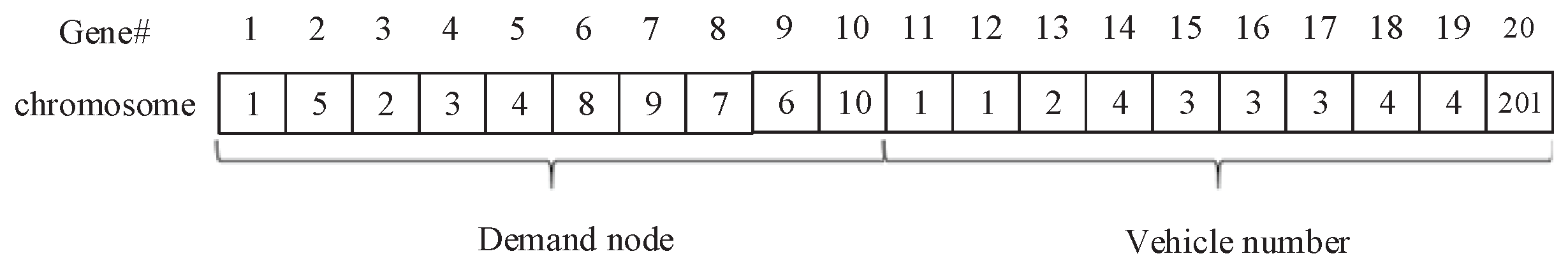
4.1.1. Chromosome Coding

The encoding method of chromosome is integer encoding, and the number of genes on chromosome is 2 | N | , where | N | is the number of demand nodes. Gene i (i [ 1 , N ] ) denotes the number of demand node, gene N + i (i [ 1 , N ] ) denotes the number of vehicle corresponding to the gene i. If | N | = 10, | M | = 3, | m 1 | = 2, and the number of own vehicles is 2; then, m M b m v m = 6 . The number of vehicles is 1 6 , where 1 b m v 1 is the number of vehicles in recycling site 1, b m v 1 + 1 b m v 1 + b m v 2 is the number of vehicles in recycling site 2, etc. When there is no owned vehicle serving demand node i, the code of gene N + i is ‘recycling site number + outside vehicle number’, where the outside vehicle number is set to s e t o v . Figure 2 illustrates a feasible chromosome.
The chromosome indicates that owned vehicle 1 travels from demand node 1 to demand node 5, owned vehicle 2 travels from demand node 2 to demand node 3, etc. Outside vehicle 01 travels from demand node 10 to recycling site 2.

4.1.2. Population Initialization

We first present two rules on the pick-up task processing sequence.
R u l e ( i ) : The sequence of genes in the first half of the chromosome is generated by sorting the demand nodes from small to large according to the right time window l i . If the right time windows of two demand nodes are equal, then the sequence is sorted from small to large according to the left time window e i . If the left and right time windows of the two demand nodes are equal, they are sorted randomly.
R u l e ( i i ) : The sequence of genes in the first half of chromosome is generated by sorting the demand nodes from small to large according to the right time window l i . If the right time windows of two demand nodes are equal, then the sequence is sorted from small to large according to the left time window e i . If the left and right time windows of the two demand nodes are equal, they are sorted randomly.
Below are detailed steps for generating the initial population of chromosomes.
S t e p 1. According to Rule (i), Rule (ii), and the random rule, different probabilities are assigned to generate the first half of the chromosome sequence achieve better quality of the initial solution on the premise of ensuring diversity of the population.
S t e p 2. For gene N+1, which denotes the number of vehicle corresponding to gene 1, we calculate the time of all vehicles that travel to this gene and then find the vehicle set k k 1 in which the elements mean that the vehicles can arrive within the time window of this gene.
S t e p 3. According to the randomly selected recycling sites, the corresponding vehicle set k k 2 is generated. Find K K = k k 1 k k 2 ; if K K , gene N + 1 is one of the members in K K randomly. If K K = , gene N + 1 is set by ’recycling site number + outside vehicle number’, where the recycling site number is the one closest to gene N + 1 in the selected recycling sites, and the outside vehicle number is randomly selected in s e t o v .
S t e p 4. For gene N + i (i ≥ 2) which denotes the number of vehicles corresponding to gene i, first, we judge if vehicle v serves other genes. If vehicle v does not serve any other genes; then, the time of arrival at gene i is the time between the recycling site to which vehicle v belongs and gene i, and the capacity of vehicle v before it arrives is Q c . If vehicle v serves another gene j before i; then, the time of arrival at gene i is m a x { T j , e j } + t j + t i j and the capacity of vehicle v before it arrives at gene i is Q c q j . If vehicle v serves two more genes before gene i; then, time of arrival at gene i is m a x { T j , e j } + t j + t i j , and the capacity of vehicle v before it arrives at gene i is the capacity of vehicle v before it arrives at gene j q j .
S t e p 5. Find out the vehicle set k k 3 in which vehicles can meet the capacity constraint and time window constraint of gene i according to S t e p 4.
S t e p 6. Find K K 1 = k k 3 k k 2 ; if K K 1 , gene N + i is an arbitrary member in K K 1 randomly. If K K 1 = , gene N + i is set by ’recycling site number + outside vehicle number’, where the recycling site number is the one closest to gene N + i in the selected recycling sites, and the number of outside vehicles is randomly selected in s e t o v .

4.1.3. Calculation of Objective Value

We calculate the objective function value according to Formulae (1), (2), and (3) and the following steps.
S t e p 1. For the sequence of genes in the last half of chromosome, we find out the set p o s i t i o n v , which contains the genes that the owned vehicle v serves. If p o s i t i o n v contains a single element, then c o s t 1 ( v ) = 2 · v c · c 1 · t N + l o c v , p o s i t i o n v . If otherwise, there are two or more elements in p o s i t i o n v , then h ( 1 ) = v c · c 1 · t N + l o c v , p o s i t i o n v ( 1 ) , while h ( 1 ) denotes the transportation cost generated when vehicle v travels to the first element. h ( r ) = h ( r 1 ) + v c · c 1 · t p o s i t i o n v ( r 1 ) , p o s i t i o n v ( r ) , where h ( r ) denotes the transportation cost generated when vehicle v travels to the r element. Therefore, c o s t 1 ( v ) = h ( e n d ) + v c · c 1 · t p o s i t i o n v ( r ) , N + l o c v . The transportation cost generated by owned vehicles when they pick up e-waste is c o s t 11 = c o s t 1 ( v ) .
S t e p 2. Find out set H s e t , which contains recycling sites. Outside vehicles travel to these recycling sites. c o s t 2 ( l ) = v c · c 1 · t H ( H s e t ( l ) ) , N + H s e t ( l ) , where l is the index of H s e t , and thus renting cost c o s t 22 = c o s t 2 ( v ) + L · c 2 , where L is the number of elements in H s e t .
S t e p 3. Find out the amount of e-waste that is picked up by owned vehicle v, and then, calculate Q ( l o c v ) , which denotes the amount of e-waste picked up in the selected recycling site. Find out set H s e t as in S t e p 2, and then, update the amount of e-waste of each selected recycling site. Moreover, calculate the total amount of e-waste in each selected recycling site by adding w m , which denotes the amount of self-delivered e-waste by customers. Lastly, calculate the times of transportation from the recycling sites to the processing centre and figure out c o s t 33 , which represents the transportation cost from recycling sites to the processing centre.
S t e p 4. Add up the total cost of the recycling network, that is, t o t a l = c o s t 11 + c o s t 22 + c o s t 33 , and output the final result.

4.1.4. Fitness Function

We use the following function f i t ( x ) to calculate the fitness value of chromosome x.
f i t ( x ) = 1 t o t a l ( x )
where t o t a l ( x ) is the objective value of chromosome x. Obviously, the larger the value of f i t ( x ) , the better the chromosome.

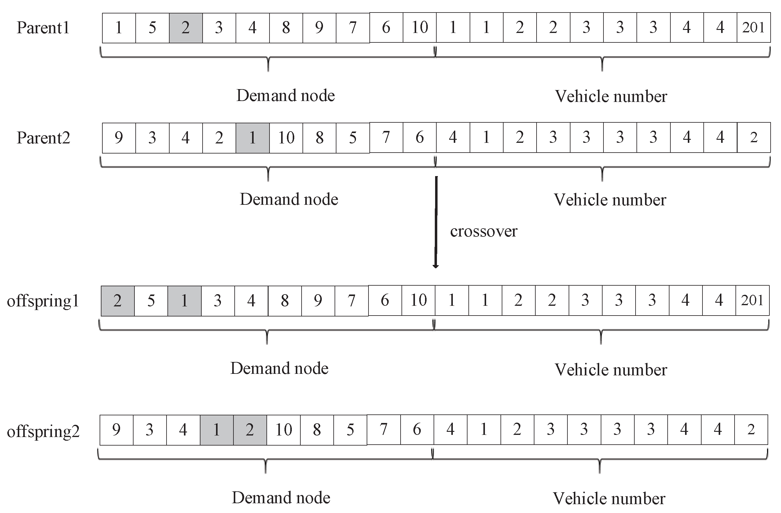
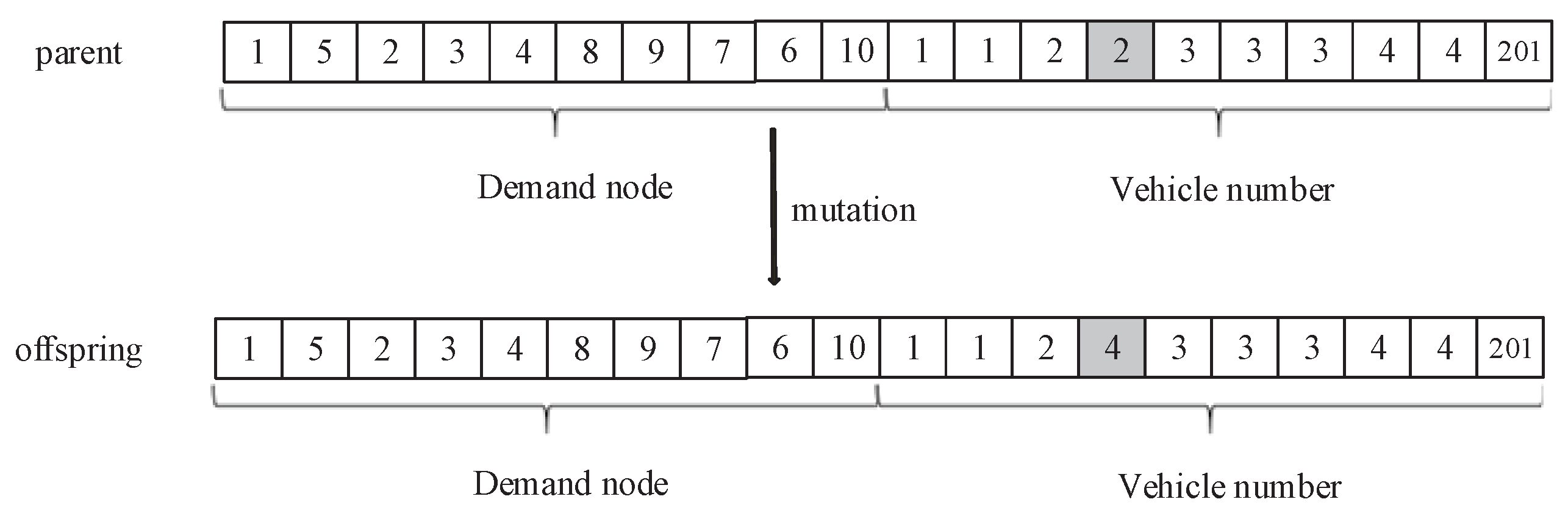
4.1.5. Genetic Operations

In each iteration of G A , chromosomes need to perform a series of genetic operations on the population, namely selection, crossover, and mutation. In our algorithm, we apply the roulette method in the selection operation.
A crossover operation refers to selecting two paternal chromosomes first and then applying a single-dot crossover approach, in which two genes from the first half of the paired chromosomes are selected to exchange genes, and the genes in the first half of the gene duplication are changed at last.
A crossover operation is shown in Figure 3. Gene 3 in parent 1 and gene 5 in parent 2 are crossed over; then, this gene is exchanged in offspring 1 and offspring 2. In contrast, gene 1 in offspring 1 and gene 4 in offspring 2 are changed to 2 and 1 in order to avoid duplication.
A mutation operation refers to the mutation of a gene in a chromosome. The mutation rule adopted in this paper is to change some gene N + i of the chromosome, that is, the service vehicle number. The variation range is within the vehicle number range of the selected recycling sites, which are given by the chromosome itself. Figure 4 shows a mutation operation, where gene 14 in parent 1 mutates. In parent 1, recycling sites 1 and 2 are selected, so the value of gene 14 in offspring 1 ranges from 1 to 4. Gene 14 in offspring 1 changes to 4 after a mutation in this instance.

4.1.6. Feasibility Judgment

It is necessary to make a feasibility judgment on whether the offsprings generated after selection, crossover, and mutation operations meet the rules of chromosome generation. The judgment includes two aspects, that is, the capacity constraint of vehicles and the time window constraint.
For the capacity constraint, we first find a set of demand nodes for each vehicle and then sum up the amount of e-waste in these demand nodes. If it exceeds Q c , implying that the offspring is infeasible, then the objective value of the offspring is set to be an infinite real number. The offspring is eliminated in the next iteration.
For the time window constraint, it is necessary to consider owned vehicles of the sites because outside vehicles always meet the time requirement due to the last assumption of the problem. We calculate the vehicle arrival time at each demand node. If the arrival time at any node exceeds its latest acceptable start time, it implies that this offspring is infeasible. Again, the objective value of the offspring is assigned by an infinite real number, and thus, it in eliminated in the next iteration.

4.1.7. Termination Condition

In the G A algorithm, we set two termination conditions: (i) it reaches the maximum iteration times M A X G E N , and (ii) the objective value of the current best solution is 0. G A terminates once either condition is met.

4.2. Heuristic Algorithm

In this section, we propose a two-stage greedy algorithm based on clustering to solve the problem effectively. The algorithm divides and the problem into two sub-problems, i.e., the location sub-problem and the routing sub-problem, and solves them iteratively. In each iteration, the output of the location sub-problem serves as the input of the routing sub-problem. The main ideas for solving the two sub-problems are described in the following two subsections.

4.2.1. The Location Sub-Problem

We first calculate the central point coordinate ( x i i , y i i ) of all the demand nodes, and it is obtained according to the K-means of Stochastic Gradient Descent ([34]). There are four steps below to obtain the location of central point ( x i i , y i i ) .
S t e p 1. Assign initial values to ( x i i , y i i ) . Calculate the mean value of each dimension of demand node coordinates ( x i , y i ), and add the random vector to the mean value, which is the initial value of the central point.
S t e p 2. Calculate the distance between each demand node ( x i , y i ) and the central point coordinate ( x i i , y i i ) ;
S t e p 3. Update central point. Select a demand node randomly, and the coordinate of the central point is close to the coordinate of the demand node by d e l t a = [ ( x i , y i ) ( x i i , y i i ) ] · e t a , where e t a is the learning rate, and the new coordinate of the central point is ( x i i , y i i ) = ( x i , y i ) + d e l t a ;
S t e p 4. Repeat the above steps. If d e l t a of the current iteration is smaller than that of the previous iteration, stop and output the best solution.
Given the coordinate of central point ( x i i , y i i ) and that of each candidate recycling site, the number of vehicles in set b m v , and the number m 1 of selected recycling sites, we calculate d i m , which denotes the distance between recycling site m and central point i and then sequence the recycling site candidates in the non-decreasing order of d m = d i m · ( 1 b m v m M b m v ) . We then select m 1 candidates with the smallest values of d m to be the final selected recycling sites in the location sub-problem.

4.2.2. The Routing Sub-Problem

S t e p 1. The set of demand nodes D is sequenced in the non-decreasing order of the latest acceptable start time l i . Ties are broken by selecting the smallest e i , i.e., the earliest acceptable start time.
S t e p 2. Determine the vehicle for serving each demand node as well as the routing of each vehicle. We first calculate the potentially earliest arrival time T i v at demand node for each vehicle v in the m 1 selected recycling sites. With the vehicle capacity constraint and time window requirement of the demand node, the vehicle v with either the smallest T i v or the smallest | e i T i v | is selected to actually serve the demand node. If there is no owned vehicle satisfying the above constraint, then the demand node is served by one outside vehicle. Along with the sequence of demand nodes in D (i.e., the sequence obtained in Step 1), the corresponding service vehicle index sequence can be produced. If the measure of smallest T i v is adopted, then the obtained vehicle index sequence is denoted by V 1 ; otherwise, if the measure of smallest | e i T i v | is used, then it is denoted by V 2 .
S t e p 3. Compare the total cost of the solution obtained by sequence V 1 and that by sequence V 2 in the routing sub-problem, and select the sequence with the smaller cost for the solution of the service vehicle routing sub-problem.

5. Computational Experiments

In the numerical experiments, MATLAB2014b is used on the personal computer with Intel (R) Core (TM) i5-8500T CPU @ 2.11GHz, and Windows 10 64-bi operating system. The exact solution obtained by solving the mathematical model is by the CPLEX12.9 solver.

5.1. Experimental Parameters

By reading the literature related to location-routing problem and reviewing the published vehicle data of relevant companies, the following parameters are given. Otherwise, some parameters (e.g., coordinate of demand nodes) are randomly generated within a reasonable range.
-
speed of vehicles: v c = 1 km/min ([35]);
-
cost of transporation per minute: c 1 = 0.5 CNY/km ([18]);
-
renting cost per time: c 2 = 200 CNY/km ([36]);
-
capacity of small vehicles: Q c = 1800 kg;
-
capacity of large vehicles: Q t = 6000 kg;
-
coordinate range of demand nodes and recycling sites: randi([10,100], | U | ,2)
-
coordinate range of the recycling centre: randi([110,150],1,2);
-
time window of demand node i: e i =randi(300,1, | N | ), c h a i = randi([20,70],1, | N | ), and l i = e i + c h a i ;
-
processing time of demand node i: t i = randi(120, 1, | N | );
-
amount of e-waste in demand node i: q i = randi([50,1000], 1, | N | );
-
amount of e-waste sent by customers in m: w i = randi([2000,3000], 1, | M | );

5.2. Numerical Results

Table 2 and Table 3 show the computational results of small-size and large-size instances. The first three columns are parameters of [ | N | , | M | ], m 1 , and b m v . Columns 4 and 5 are results related to CPLEX. Columns 6, 7, and 8 are results related to GA. Additionally, the last three column are results related to TSGL. Among them, Obj denotes the objective function value of each instance, G a p 1 = G A C P L E X C P L E X 100 % and G a p 2 = T S G L G A G A 100 % , where A v g denotes the mean value of each group that consists of seven instances.
By Table 2, it can be concluded that CPLEX can obtain optimal values in most small-scale cases. However, for large-scale instances, CPLEX cannot output even feasible solutions within the limited time (i.e., 2 h). When scale increases, the run time of CPLEX increases rapidly from 1.4 s to 7200 s. The run time of GA also increases with the increase in scale, but the feasible solution can be obtained in a short time while the time of the heuristic algorithm is very short, and the feasible solution can be obtained in 2 s. In terms of the quality of the solution, optimal values can be obtained, such as in the first and second groups of examples, and G a p 1 is 0. With the increase in size, the gap between the feasible solution and the optimal solution gradually increases. It can be seen that the average gap between GA and the exact solution obtained by CPLEX for each group of instances is between 0% and 18.6% and that the average gap between TSGL and GA is between 8.4% and 28.9%. The average gap between GA and CPLEX is about 7.0% in total, and the average gap between TSGL and GA algorithm is about 17.8% in total.
Table 2 shows the experimental results of large-scale instances. Since the CPLEX solver cannot obtain the optimal value within 7200 s for the large-scale instances, the results of GA algorithm and heuristic algorithm are only compared and analyzed. It can be seen from the run time that GA increases gradually with the increase in the scale. The average run time of each group is between 37.1 s and 90.4 s while the run time of the heuristic algorithm is very stable, and the average time is between 0.9 s and 1.8 s. It can be seen that the solving time of the heuristic algorithm is much shorter than that of the genetic algorithm. In terms of the objective value, the average gap of large-scale instances is between 5.3% and 20.6%.

6. Conclusions

This paper presents an optimization model of an e-waste recycling network when considering renting social idle vehicles. In order to meet all of the demands of demand nodes within their expected time windows, with a limited number of own vehicles, idle social vehicles are allowed to be rented in the sharing economy environment to reduce the total operating cost of the recycling logistics network. Meanwhile, both the selection of recycling sites and the delivery routes of owned vehicles need to be determined. The genetic and a two-stage greedy algorithm are proposed to solve the problem, and numerical results demonstrate the effectiveness of two algorithms by small-scale and large-scale instances.
In a recycling network, the recycling sites and owned vehicles equipped need large amounts of capital investment. As a result, it is essential to decide the locations of recycling sites on the basis of recycling demands. Considering renting social idle vehicles when recycling demands surge, leading to a shortage of owned vehicle, is wise and economic because it only costs a small rental fee compared with equipping more vehicles for service.
This study is limited in that the processing time of recycling in demand nodes and the number of demand nodes are considered deterministic. To address this limitation, developing a random and undetermined model of the e-waste recycling location routing problem is a worthwhile topic for future research. Otherwise, another direction for future research is considering multi-objective location routing problems. Last but not the least, from a solution approach perspective, more efficient heuristic or meta-heuristic algorithms should be developed for the considered problem.

Author Contributions

Conceptualization, F.Z., Z.S. and M.L.; methodology, Z.S. and M.L.; software, Z.S.; validation, F.Z., Z.S. and M.L.; formal analysis, F.Z., Z.S. and M.L.; investigation, F.Z., Z.S. and M.L.; resources and data curation, F.Z., Z.S. and M.L.; writing—original draft preparation, Z.S.; writing—review and editing, F.Z., Z.S. and M.L.; visualization, F.Z. and Z.S.; supervision, F.Z. and M.L.; project administration, F.Z. and M.L.; funding acquisition, F.Z. All authors have read and agreed to the published version of the manuscript.

Funding

This research was funded by National Natural Science Foundation of China grant number 71771048 and the Fundamental Research Funds for the Central Universities grant number 2232018H-07.

Institutional Review Board Statement

Not applicable.

Informed Consent Statement

Not applicable.

Acknowledgments

This work was partially supported by the National Natural Science Foundation of China (grant No. 71771048) and the Fundamental Research Funds for the Central Universities (2232018H-07).

Conflicts of Interest

The authors declare no conflict of interest.

References

  1. Li, W.; Achal, V. Environmental and health impacts due to e-waste disposal in china—A review. Sci. Total Environ. 2020, 737, 139745. [Google Scholar] [CrossRef] [PubMed]
  2. Thompson, R.G.; Nassir, N.; Frauenfelder, P. Shared freight networks in metropolitan areas. Transp. Res. Procedia 2020, 57, 204–211. [Google Scholar] [CrossRef]
  3. Salhofer, S.; Steuer, B.; Ramusch, R.; Beigl, P. WEEE management in Europe and China—A comparison. Waste Manag. 2016, 57, 27–35. [Google Scholar] [CrossRef] [PubMed]
  4. Singh, N.; Li, J.; Zeng, X. Solutions and challenges in recycling waste cathode-ray tubes. J. Clean. Prod. 2016, 133, 188–200. [Google Scholar] [CrossRef]
  5. Guo, J.; Tang, B.; Huo, Q.; Liang, C.; Gen, M. Fuzzy programming of dual recycling channels of sustainable multi-objective waste electrical and electronic equipment (WEEE) based on triple bottom line (TBL) theory. Arab. J. Sci. Eng. 2021, 1–14. [Google Scholar] [CrossRef]
  6. He, K.; Sun, Z.; Hu, Y.; Zeng, X.; Yu, Z.; Cheng, H. Comparison of soil heavy metal pollution caused by e-waste recycling activities and traditional industrial operations. Environ. Sci. Pollut. Res. 2017, 24, 1299–1332. [Google Scholar] [CrossRef] [PubMed]
  7. Cao, J.X.; Zhang, Z.X.; Zhou, Y.G. A location-routing problem for biomass supply chains. Comput. Ind. Eng. 2021, 152, 107017. [Google Scholar] [CrossRef]
  8. Gamberini, R.; Gebennini, E.; Manzini, R.; Ziveri, A. On the integration of planning and environmental impact assessment for a WEEE transportation network—A case study. Resour. Conserv. Recycl. 2010, 54, 937–951. [Google Scholar] [CrossRef]
  9. Nowakowski, P. A proposal to improve e-waste collection efficiency in urban mining: Container loading and vehicle routing problems—A case study of Poland. Waste Manag. 2017, 145, 494–504. [Google Scholar] [CrossRef] [PubMed]
  10. Beneventti, G.D.; Bronfman, C.A.; Paredes-Belmar, G.; Marianov, V. A multi-product maximin hazmat routing-location problem with multiple origin-destination pairs. J. Clean. Prod. 2019, 240, 118193. [Google Scholar] [CrossRef]
  11. Sakti, S.; Yu, V.F.; Sopha, B.M. Heterogeneous fleet location routing problem for waste management: A case study of Yogyakarta, Indonesia. Int. J. Inf. Manag. Sci. 2019, 30, 1–16. [Google Scholar]
  12. Zhao, J.; Ke, G.Y. Incorporating inventory risks in location-routing models for explosive waste management. Int. J. Prod. Econ. 2017, 193, 123–136. [Google Scholar] [CrossRef]
  13. Dukkanci, O.; Kara, B.Y.; Bektas, T. The green location-routing problem. Comput. Oper. Res. 2019, 105, 187–202. [Google Scholar] [CrossRef]
  14. Zhou, L.; Wang, X.; Lin, N. Location-Routing problem with simultaneous home delivery and customer’s pickup for city distribution of online shopping purchases. Sustainability 2016, 8, 828. [Google Scholar] [CrossRef] [Green Version]
  15. Ng, A.; Agp, B.; Ob, A.; Mv, C. The multi-depot open location routing problem with a heterogeneous fixed fleet. Expert Syst. Appl. 2020, 165, 113846. [Google Scholar] [CrossRef]
  16. Vandani, B.; Mousavi, S. A robust approach to multiple vehicle location-routing problems with time windows for optimization of cross-docking under uncertainty. J. Intell. Fuzzy Syst. Appl. Eng. Technol. 2017, 32, 49–62. [Google Scholar]
  17. Kuroki, H.; Ishigaki, A.; Takashima, R. A location-routing problem with economic efficiency for recycling system. Procedia Manuf. 2020, 43, 215–222. [Google Scholar] [CrossRef]
  18. Pourhejazy, P.; Zhang, D.; Zhu, Q.; Wei, F.; Song, S. Integrated E-waste transportation using capacitated general routing problem with time-window. Transp. Res. Part Logist. Transp. Rev. 2021, 145, 102169. [Google Scholar] [CrossRef]
  19. Agnusdei, G.P.; Gnoni, M.G.; Tornese, F. Modelling and simulation tools for integrating forward and reverse logistics: A literature review. In Proceedings of the European Modeling & Simulation Symposium, Lisbon, Portugal, 18–20 September; pp. 317–326.
  20. Abid, S.; Radji, S.; Mhada, F.Z. Simulation techniques applied in reverse logistic: A review. In Proceedings of the 2019 International Colloquium on Logistics and Supply Chain Management (LOGISTIQUA), Paris, France, 12–14 June 2019; pp. 1–6. [Google Scholar]
  21. Surekha, P.; Sumathi, S. Solution to multi-depot vehicle routing problem using genetic algorithms. World Appl. Program. 2011, 1, 118–131. [Google Scholar]
  22. Yang, J.; Sun, H. Battery swap station location-routing problem with capacitated electric vehicles. Comput. Oper. Res. 2015, 55, 217–232. [Google Scholar] [CrossRef]
  23. Berglund, P.G.; Kwon, C. Robust facility location problem for hazardous waste transportation. Netw. Spat. Econ. 2014, 14, 91–116. [Google Scholar] [CrossRef]
  24. Ferdi, I.; Layeb, A. A grasp algorithm based new heuristic for the capacitated location routing problem. J. Exp. Theor. Artif. Intell. 2018, 30, 369–387. [Google Scholar] [CrossRef]
  25. Almouhanna, A.; Quintero-Araujo, C.L.; Panadero, J.; Juan, A.A.; Ouelhadj, D. The location routing problem using electric vehicles with constrained distance. Comput. Oper. Res. 2019, 115, 104864. [Google Scholar] [CrossRef]
  26. Schiffer, M.; Walther, G. The electric location routing problem with time windows and partial recharging. Eur. J. Oper. Res. 2017, 260, 995–1013. [Google Scholar] [CrossRef]
  27. Ponboon, S.; Qureshi, A.G.; Taniguchi, E. Branch-and-price algorithm for the location-routing problem with time windows. Transp. Res. Part Logist. Transp. Rev. 2016, 86, 1–19. [Google Scholar] [CrossRef]
  28. Pichka, K.; Bajgiran, A.H.; Petering, M.E.; Jang, J.; Yue, X. The two echelon open location routing problem: Mathematical model and hybrid heuristic. Comput. Ind. Eng. 2018, 121, 97–112. [Google Scholar] [CrossRef]
  29. Lopes, R.B.; Ferreira, C.; Santos, B.S. A simple and effective evolutionary algorithm for the capacitated location-routing problem. Comput. Oper. Res. 2016, 70, 155–162. [Google Scholar] [CrossRef]
  30. Kilic, H.S.; Cebeci, U.; Ayhan, M.B. Reverse logistics system design for the waste of WEEE in Turkey. Resour. Conserv. Recycl. 2015, 95, 120–132. [Google Scholar] [CrossRef]
  31. Zhang, S.; Chen, M.; Zhang, W. A novel location-routing problem in electric vehicle transportation with stochastic demands. J. Clean. Prod. 2019, 221, 567–581. [Google Scholar] [CrossRef]
  32. Gen, M.; Syarif, A. Hybrid genetic algorithm for multi-time period production/distribution planning. Comput. Ind. Eng. 2005, 48, 799–809. [Google Scholar] [CrossRef]
  33. Hu, H.; Li, X.; Zhang, Y.; Shang, C.; Zhang, S. Multi-objective location-routing model for hazardous material logistics with traffic restriction constraint in inter-city roads. Comput. Ind. Eng. 2018, 128, 861–876. [Google Scholar] [CrossRef]
  34. Cinar, D.; Gakis, K.; Pardalos, P.M. A 2-phase constructive algorithm for cumulative vehicle routing problems with limited duration. Comput. Ind. Eng. 2016, 56, 48–58. [Google Scholar] [CrossRef]
  35. Bektaş, T.; Laporte, G. The pollution-routing problem. Transp. Res. Part B Methodol. 2011, 45, 1232–1250. [Google Scholar] [CrossRef]
  36. Xie, H. Research on Strategic Choice and Development in A Car Rental Company; Tianjin University: Tianjin, China, 2016. [Google Scholar]
Figure 1. Illustration of an e-waste recycling network.
Sustainability 13 11879 g001
Figure 2. A feasible chromosome.
Sustainability 13 11879 g002
Figure 3. Crossover operation.
Sustainability 13 11879 g003
Figure 4. Mutation operation.
Sustainability 13 11879 g004
Table 1. Comparison of research in the location routing problem.
ReferencesObjectiveVehicle FleetVehicle CapacityTime WindowSolution Method
Cao et al. [7]min FEC & TCsingle--CPLEX,TS
Nowakowski [9]min TCsingle-GLSA
Zhao et al. [12]min TC, FEC & risksingle-TOPSIS
Beneventtiet et al. [10]max MWD; min THIP, FEC & TCsingle--CPLEX
Dukkanci et al. [13]min FEC, FC & CO 2 Csingle-ILSA
Zhou et al. [14]min FEC, TC & SDCsingleHESA
Ng et al. [15]min TCsingle-MA
Vandani et al. [16]min TC & ICmultiMA
Kuroki et al. [17]min RC & TCsingle--SAA
Pourhejazy et al. [18]max TPsingleTS
this studymin FC & RSVCmultiCPLEX, GA, HA
Note: TC: transportation cost; FEC: facility establishment cost; RC: recycling cost; MWD: the minimum weighted distance; THIP: the total hazardimposed on the non-vulnerable population; FC and CO 2 C: fuel and CO 2 emissions cost; SDC: the second delivery cost; IC: inventory cost; RSVC: renting social vehicles cost; TP: total profit; TS: Tabu search; GA: genetic algorithm; MA: metaheuristic algorithm; HA: heuristic algorithm; HESA: hybrid evolution search algorithm; ILSA: iterated local search algorithm; GLSA: greedy and local search algorithm; SAA: simulated annealing algorithm.
Table 2. Computational results of small-scale instances.
InstancesCPLEXGATSGL
[ | N | , | M | ] m 1 b m v Obj Time Obj Time Gap 1 Obj Time Gap 2
1[1,1]584.01.1584.09.30.0584.00.20.0
2[1,1]259.51.1259.59.70.0267.00.32.9
1[2,2]208.01.4208.010.60.0216.00.33.6
[5,2]2[2,2]208.01.4208.010.60.0216.00.33.6
1[1,1]259.51.1259.59.70.0267.00.32.9
1[1,2]432.51.3432.510.70.0584.00.335.0
2[1,2]259.51.3259.510.30.0267.00.32.9
no time windows, m 1 = 1146.51.5146.510.40.0162.50.310.9
Avg299.91.3299.910.20.0328.10.48.4
2[1,1,1]1159.53.41159.511.10.01166.50.40.6
3[1,1,1]853.03.5853.012.30.0934.50.49.5
2[2,2,2]437.55.3437.514.00.0443.50.41.4
[10,3]3[2,2,2]437.57.7437.514.30.0443.50.41.4
2[2,1,3]451.55.3451.514.30.0558.50.423.8
3[2,1,3]451.55.3451.514.30.0558.50.423.8
no time windows, m 1 = 2314.521.2314.513.40.0343.00.49.1
Avg586.47.4586.413.40.0635.40.49.9
2[2,2,2,2,2]897.0278.31064.517.918.71107.50.54.0
3[2,2,2,2,2]378.026.1398.019.45.3581.50.446.1
2[3,3,3,3,3]392.025.4399.521.41.9541.00.535.4
[15,5]3[3,3,3,3,3]375.537.7379.523.01.0579.50.552.7
2[2,3,2,3,1]506.538.7522.020.03.1585.50.512.2
3[2,3,2,3,1]439.034.5465.520.36.1572.00.522.9
no time windows, m 1 = 2756.0832.4792.017.54.8820.00.53.5
Avg498.073.5538.220.36.0661.20.528.9
2[2,2,2,2,2]1678.51516.91977.019.017.82220.50.712.3
3[2,2,2,2,2]899.54639.31107.521.023.11148.50.73.7
2[3,3,3,3,3]--1024.523.3-1054.50.72.9
[20,5]3[3,3,3,3,3]476.0734.5507.526.56.6724.50.642.8
2[2,3,2,3,2]930.01157.61102.518.540.11202.00.69.0
3[2,3,2,3,2]511.0354.7538.023.85.3743.00.738.1
no time windows, m 1 = 2--834.037.9-850.51.52.0
Avg899.01680.61013.024.318.61134.80.815.8
3[2,2,2,2,2,2,2,2]--1285.024.8-1356.51.25.6
4[2,2,2,2,2,2,2,2]523.5270.0621.026.118.6724.50.616.7
3[2,2,2,2,2,2,2,2]524.0841.7579.530.510.6744.51.128.4
[20,8]4[2,2,2,2,2,2,2,2]520.0571.1547.832.75.3744.50.635.9
3[2,2,2,2,2,2,2,2]569.03169.2602.027.55.8776.50.629.0
4[2,2,2,2,2,2,2,2]522.0135.8582.026.711.5822.50.641.3
no time windows, m 1 = 2--543.228.9-682.00.725.6
Avg531.7997.6680.128.210.4835.90.826.1
Table 3. Computational results of large-scale instances.
InstancesGATSGL
[ | N | , | M | ] m 1 b m v Obj Time Obj Time Gap 2
3[2,2,2,2,2,2,2,2]1616.034.81719.51.06.4
4[2,2,2,2,2,2,2,2]1146.339.81193.51.14.1
3[3,3,3,3,3,3,3,3]683.446.5851.01.124.5
[25,8]4[3,3,3,3,3,3,3,3]708.048.8847.01.119.6
3[3,2,2,3,2,2,2,3]891.630.8944.00.75.9
4[3,2,2,3,2,2,2,3]703.932.5778.00.810.5
Avg958.238.91055.51.06.1
4[2,2,2,2,2,2,2,2,2,2]1786.232.51872.01.14.8
5[2,2,2,2,2,2,2,2,2,2]1244.635.51462.50.917.5
4[3,3,3,3,3,3,3,3,3,3]1018.842.61218.50.919.6
[35,10]5[3,3,3,3,3,3,3,3,3,3]902.645.21345.50.949.1
4[2,2,1,2,1,3,1,2,1,2]2504.230.42917.50.816.5
5[2,2,1,2,1,3,1,2,1,2]1709.036.51986.50.816.2
Avg1527.637.11800.40.920.6
5[2,2,2,2,2,2,2,2,2,2,2,2]2618.658.92667.51.61.9
6[2,2,2,2,2,2,2,2,2,2,2,2]1669.366.21709.51.62.4
5[3,3,3,3,3,3,3,3,3,3,3,3]1204.682.11360.01.612.9
[45,12]6[3,3,3,3,3,3,3,3,3,3,3,3]1155.488.91383.01.619.7
5[2,3,4,2,3,2,2,2,2,3,2,3]1256.575.81310.51.64.3
6[2,3,4,2,3,2,2,2,2,3,2,3]1305.577.81415.01.68.4
Avg1535.075.01640.91.67.1
6[2,2,2,2,2,2,2,2,2,2,2,2,2,2]2919.071.43013.01.83.2
7[2,2,2,2,2,2,2,2,2,2,2,2,2,2]2118.477.22554.01.920.6
6[3,3,3,3,3,3,3,3,3,3,3,3,3,3]1338.398.01474.01.810.1
[50,14]7[3,3,3,3,3,3,3,3,3,3,3,3,3,3]1188.4103.51343.51.813.1
6[2,3,4,3,2,3,3,3,3,3,2,3,2,3]1377.896.21576.51.814.4
7[2,3,4,3,2,3,3,3,3,3,2,3,2,3]1318.195.91369.01.83.9
Avg1710.090.41888.31.810.9
7[2,2,2,2,2,2,2,2,2,2,2,2,2,2,2,2]3227.256.23324.01.33.0
8[2,2,2,2,2,2,2,2,2,2,2,2,2,2,2,2]2495.960.62514.51.30.7
7[3,3,3,3,3,3,3,3,3,3,3,3,3,3,3,3]1708.678.21840.51.47.7
[55,16]8[3,3,3,3,3,3,3,3,3,3,3,3,3,3,3,3]1672.282.21815.01.58.5
7[2,3,2,2,3,3,1,2,1,2,3,2,2,3,3,2]1934.164.42054.01.56.2
8[2,3,2,2,3,3,1,2,1,2,3,2,2,3,3,2]1716.469.51813.51.25.7
Avg2125.768.52226.91.45.3
Publisher’s Note: MDPI stays neutral with regard to jurisdictional claims in published maps and institutional affiliations.

