Abstract
Decarbonization of the UK residential heating sector is crucial to cut the carbon emissions and meet the legal binding of the Climate Change Act, 2008. The current progress with residential building sector carbon neutrality is slow and, hence, acceleration in action is required. The heat pump (HP) technology was found to be a potential candidate for sustainable development instead of fossil fuel-based oil/gas boilers, but improvement in its coefficient of performance (COP) is essential to compete with the lower gas/oil unit energy cost. The number of studies found in the literature were very limited, with the customized prototype development in the context of Northern Ireland, but without considering the simultaneous impact of heat supply temperature and operating mode of control for performance improvement in different property types. It is evidenced in the literature that the variable speed capacity control approach could improve the annual performance, but the literature has not looked into the compressor efficiencies challenges. In this study, steady state testing with a range of fixed constant heat loads (3–18 KW), done by varying compressor speed and its impact on COP, compressor efficiencies, and inverter losses, was established. The HP performance was measured and evaluated at low (35 °C)-to-medium (45 °C) and high (55 °C) heat supply temperature levels under the controlled laboratory conditions over the experienced ambient temperature. According to the result the COP values varies according to heat supply temperature, ambient temperature conditions, and heating capacity. The HP annual performances with Irish housing stock were evaluated in two modes of control and three case studies (C1, C2, C3) based on the experimentally validated model. The heat load demand in five property types with four age periods were considered in the analysis. The system could meet the required heat load demand for all property types in VSM with different percentage improvements in performance in comparison to FSM depending on the considered case level of the heat supply temperature (C1, C2, C3).
1. Introduction
The building sector was responsible for 38% of total greenhouse gas (GHG) emissions globally, with a share of 17% from residential buildings in 2019 [1]. The European Union (EU) countries’ building sector contributes 36% of the total final carbon emissions [2]. Similarly, the UK residential building sector consumes 29% of the total final energy consumption [3] and adds 16% of the total CO2 emitted into the atmosphere [4]. A major portion of the energy consumption (79%) inside residential building goes to space heating (SH) and domestic hot water (DHW) production in the UK [5]. This contributes 40% of total carbon emission among residential buildings in the UK [6]. Hence, there is a great potential of carbon emission reduction if the residential building heating demand could be met by renewable-based energy devices instead of fossil fuel-based boilers. The recent International Energy Agency (IEA) report recommends the ban of sale of fossil fuel boilers from 2025 to achieve the target of net-zero emissions by 2050 [7]. The UK, as a signatory of Climate Change Act 2008, set the target of net-zero carbon emissions by 2050 [8,9], and banned the sale of fossil fuel-based boilers by 2025 [10]. The HP technology utilizes environmental thermal heat energy from the air/ground, with some proportion of electrical energy. The air source heat pump (ASHP) has a lower initial capital cost and less disruption with installations inside the existing buildings, compared to the ground source heat pump (GSHP) system. Hence, it is more favorable for domestic retrofit and has great potential for market penetrations in the context of Ireland [11]. The high starting current and temperature control due to its intermittent operation were among the barriers in the promotion of the HP technology uptake at large scale [12]. The restart of the unit with intermittent operation causes high current consumption because of compressor pressures’ re-establishment. The on/off controlled systems synchronized operation at a large scale can cause network failure. The risk of network instability because of additional current load increases with back-up electric heater [13]. The control of the system at part loads conditions basically differentiates variable speed drive from the conventual fixed speed system. In addition to the control challenges, the issue with ASHP system is its performance degradation at lower ambient temperature conditions and more compressor work is required, putting extra pressure on network. The HP design for meeting the highest peak load demand requires larger component sizes, with increased cost, and negative impacts the overall system performance due to higher cycling losses during the off-peak period. The peak load demand occurs only for the limited period of the year, and the idle operation of the system for the remaining period causes losses and fluctuations. In seeking a system that can modulate its capacity according to the load requirements and operate over a wide range, a variable speed compressor-based HP system is a viable option. The COP is improved using a variable speed compressor due to heat supply match to that of demand at part loads, resulting in lower cycling losses and reduced back-up electric heater requirements. This results in higher thermal comfort and better compressor life due to the less deteriorating effect. The building heat load demand and the system operation over the balance point for a great portion of the building load could be achieved with variable speed of control. The variable speed compressor-based HP system fulfills the heating demand at the lowest ambient temperature conditions by increasing the speed and avoids the needs for oversizing. In this study the HP potential performance improvement for the old aged Irish housing stock was investigated with the challenges to the compressor. Performance assessment of the 9 KW heat pump (HP) via testing and modeling was conducted. Impact of varying heating capacities on the system coefficient of performance (COP) at low (35 °C)-to-medium (45 °C) and high heat supply temperature (55 °C) at individual steady state tested conditions. HP annual performance improvement due to heat supply temperature level & control mode of operations (variable speed mode (VSM) vs. fixed speed mode (FSM)) for capacity adjustments were investigated. Detached, Semi-detached, Mid terraced, End terraced, and Flat property types with four age period ranging from very old to new properties were considered.
1.1. Literature Review
The current standard BS EN14511 classifies the HP system depending on the heat supply temperature level as low (35 °C), medium (45 °C), high (55 °C), and very high temperature (above 65 °C) (BS EN14511) [14]. The COP for ASHP ranges between 3.2 and 4.5, according to lab scale tests as per BS EN14511 at the lower heat supply temperature of 35 °C [15]. The HP operates continuously at partial loads to follow the building load demand during the VSM of control, which was found to be more efficient, in contrast to the conventional way of controlling the heating capacity with the load adjustment [16,17,18]. Faster temperature control, low starting current, noise, vibrations, and continuous control while meeting load demand with rare transient losses were well-established advantages of VSM against FSM [19,20,21]. The back-up electric heating requirements and its impact on the overall system performance was investigated with both control modes in [22]. The overall COP was reduced with the use of the back-up electric requirements with increased pressure on the network. The heat supply temperature with intermittent control during the on-cycle needs to be higher compared to the continuous system operation, leading to lower performance and higher energy consumption [23]. The three climatic conditions of Italy (Milan, Rome, Palermo) were investigated in [24]. Significant energy savings were achieved with variable speed control specifically in Palermo and Rome during the heating seasons due to idle operation of the system for most of the time. A comparative study between the variable speed and on/off control reported a COP improvement in the range of 10–25% [25,26,27,28]. The COP improved using a variable speed compressor due to the heat supply match to that of the demand at part loads, resulting in lower cycling losses and back-up electric heater requirements. An air to air-type heat pump with 8.8 KW nominal capacity was tested under the laboratory conditions at a range of compressor speeds, relative humidity values, and ambient conditions [29]. Based on the testing results, the transient losses were calculated for the seasonal performance evaluations and energy savings due to speed modulations. The payback period reported was three years due to additional control devices. This also causes higher thermal comfort and better compressor life due to a less deteriorating effect [30]. Comparative studies for the two modes of HP capacity control were made at different levels, including the annual performance, and at individual steady state-tested conditions with an optimal speed of operation. The annual performance comparison was found to be more valuable than the individual conditions’ performance analysis [31]. Annual performance improvement in the range of 10–25% was reported depending on the HP type (ground/air source) of compressor used, operating speed range, and design load [31]. The reason for performance improvement was because of the better part load condenser and evaporator efficiency, smaller number of cycles, back-up electric heater requirements, lower losses due to defrosting, and supply temperature [31,32]. A theoretical analysis to investigate the best approach for capacity control concluded that the varying compressor speed approach was more efficient and was studied experimentally in more detail [33]. The heat supply temperature with intermittent operations during the on-cycle needs to be higher compared to the continuous system operation, leading to high energy consumption due to higher condensation and lower evaporation temperature [23]. The climatic conditions and the associated benefits with VSM were found to be interlinked, with higher performance improvement in warm climate conditions due to idle operations of the system for most parts of the year [24]. A limited number of articles were found investigating performance improvement and energy savings with the control mode and considering heat supply temperature simultaneously for other HP types [21,31,34]. The GSHP was investigated under the laboratory conditions with a hydronic heating distribution system, aimed at increased system performance due to capacity control approaches and the selected heat supply temperature [31,34]. The reduction in heat supply temperature from high (55 °C) to low (35 °C) results in an improvement in the seasonal performance factor by 30–35% [31]. Three types hydronic heating distribution systems, i.e., underfloor, fan-assisted hydronic coil unit, and traditional wet radiator, were considered in analysis for the comparative study between VSM and FSM. The thermal inertia of various hydronic heating distribution system influences the cyclic properties of HP, response time at start-up, and consequently its overall performance [34]. The negative impact due to cycling get reduced with the VSM of control because of load matching with the heat supplied [31]. The overshoot and undershoot of the room temperature become a great concern during the intermittent operation, specifically with the underfloor heating system due to high thermal inertia. A couple of experimental studies on the variable speed compressor-based HP system with applications for industrial plant cold storage was conducted for the energy-saving potential [35,36]. The control of cooling capacity with the variable speed compressor using the fuzzy logic control algorithm instead of the thermostatic control method could save energy up to 20% [35]. The optimal speed of 24 Hz, satisfying the load demand with the supply temperature of 34 °C, could save approximately 30% of energy compared to that of the nominal speed [36]. However, there were certain issues during HP operation with the varying compressor speed compared to the nominal speed of operation, i.e., compressor isentropic, volumetric efficiency, pressure ratio, discharge line temperature, and inverter losses [37]. The isentropic efficiency was highest at 65% at the nominal speed with the pressure ratio of 2.2, while the volumetric efficiency linearly degraded from 98% to 83% with the pressure ratio variation range between 1.5 and 5.6 due to varying speed (35–75 HZ) [37]. The inverter losses due to change in compressor-supplied frequency were analyzed experimentally for GSHP and were reduced as a percentage of the total electric power consumption with the increase of speed, while keeping a constant load/source side temperature of 26 °C/4.5 °C with a frequency variation range in between 30 Hz and 90 Hz [38]. The analysis of low-to-medium and high heat supply temperatures on variable speed compressor-based ASHP was conducted at different steady state test conditions aiming for Irish housing stock retrofit applications [39]. The COP value improved in range of 30–40% due to the heat supply temperature reduction from 55 °C to 35 °C for the individual tested conditions’ range. The ASHP system with a nominal heating capacity of 9.8 KW was developed aiming at retrofit applications for old age 1900s mid-terraced houses in Belfast climatic conditions [40]. The performance was evaluated at a very high heat supply temperature of 60 °C for the experienced ambient conditions’ range under the laboratory conditions [40]. The limited frequency modulation range between 37.5 HZ and 75 HZ, resulted in a poor load match to the heat supplied during the VSM of control with an annual COP of 2.15. The short version of the study is presented in the authors’ other work [41,42].
1.2. Research Gaps and Contribution of This Work
Based on the above literature review, it can be seen that ASHP prototype development, simulating constant domestic heat loads under the controlled laboratory conditions and investigating the impact of compressor speed variations on its efficiencies and discharge line temperature at low-to-medium and high heat supply temperature levels, is missing from the literature. The application of such units for the Irish housing stock and the annual performance evaluation at low-to-medium and high heat supply temperature in two modes of control for capacity adjustment are missing from the literature to the best of authors’ knowledge. The earlier comparative studies with FSM and VSM for capacity control were performed either under single steady state conditions or investigating individual component analysis (i.e., compressor isentropic and volumetric efficiencies, inverter losses) and performance improvement at a single heat supply temperature level. Therefore the major research questions investigated in this study could be summarized as the following: (i) ASHP design, development, and testing at fixed heat loads at low-to-medium and high heat supply temperatures and experienced ambient temperature conditions; (ii) numerical modeling of the HP performance based on testing results and validations; (iii) the annual performance improvement and energy savings with VSM in comparison to FSM for Irish housing stock; (iv) part load operation and the importance of balance point with different property types in two modes of control and at three levels of HP supply temperature.
2. Methodology
2.1. Heat Pump Characterizations
The developed domestic ASHP protype was characterized with the required test conditions established inside the conditioning chamber with constant heat load demands. The test facility could provide a range of ambient temperatures and humidity conditions on the source side and the required set points values for EWT/WST by using PID controllers. The HP system was developed and installed at a test facility with a variable speed scroll compressor, superheat and envelope controller, and other parts purchased from Emerson Climate Technologies. The modulation range for the tested compressor was in between 15 Hz and 120 Hz. The controller developed for XPV/XHV for heating and cooling applications provided the function of map management and compressor speed with the refrigerant R410a. The superheat set point was 10 K during all the tests and it was maintained by using an electronic expansion valve. The parts’ details are mentioned in Table 1.

Table 1.
List of the main components for the developed system with model number.
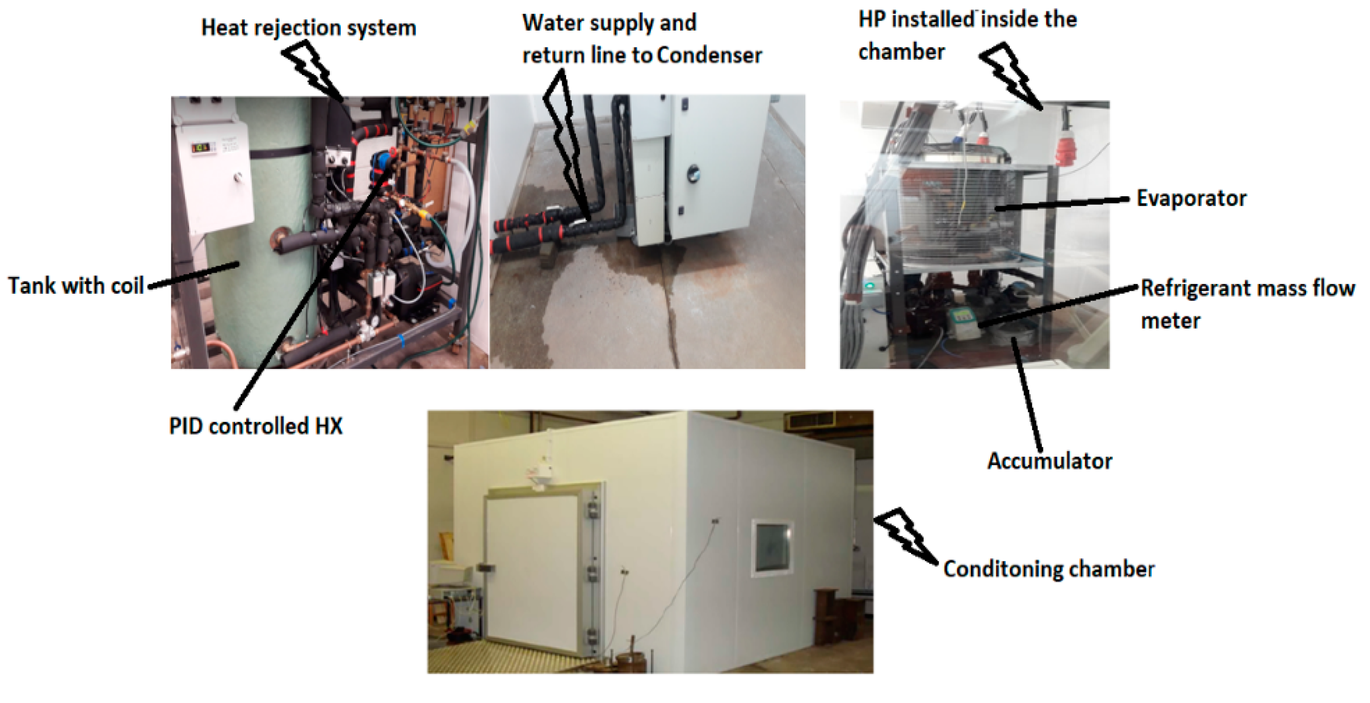
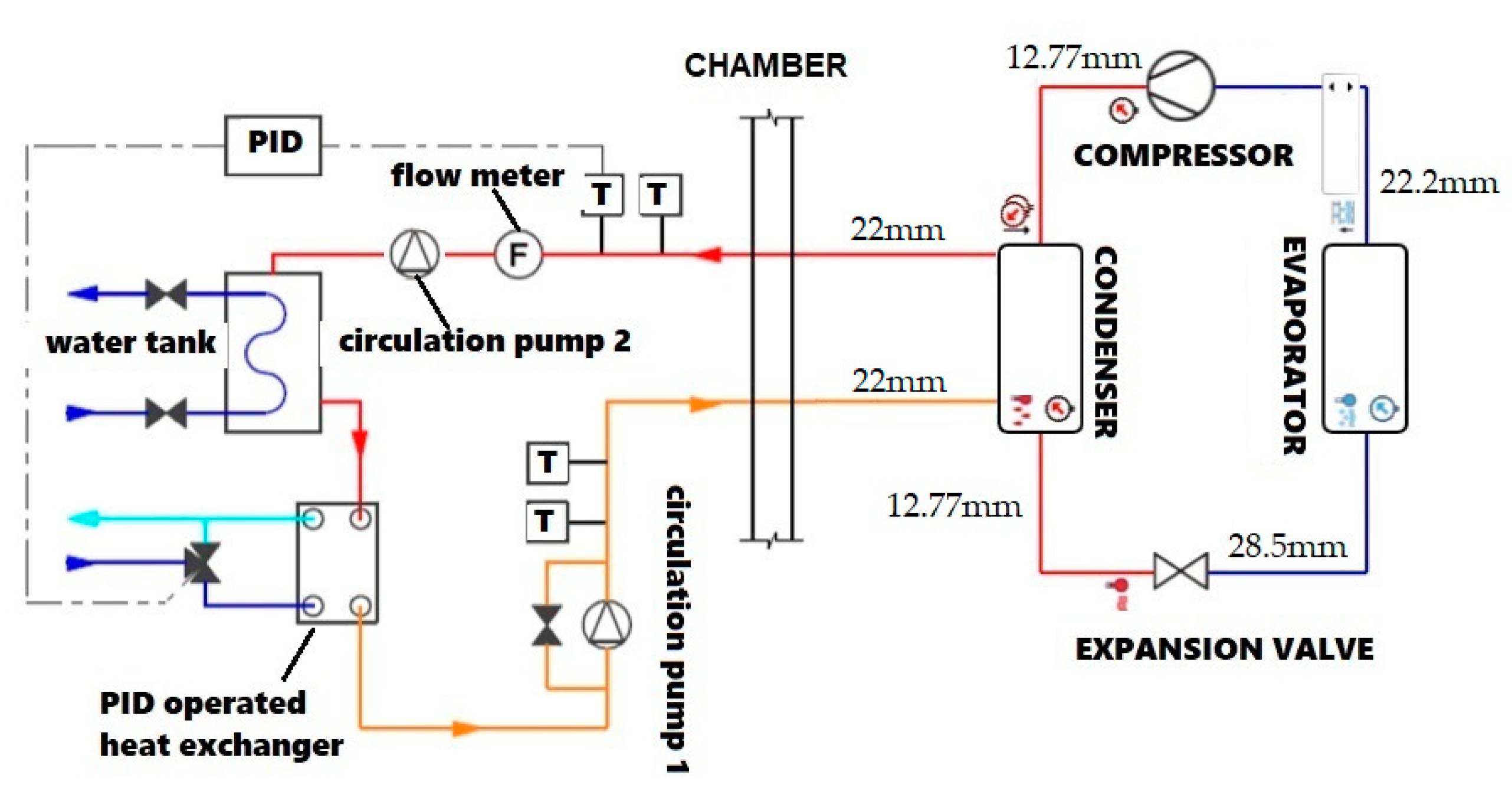
The experimental setup pictorial view with a simplified schematic diagram is shown in Figure 1. The pictorial view shows the heat rejection system, water supply, and return line to the condenser, and the heat pump system inside the conditioning chamber. The schematic diagrams show that the test rigs basically consist of three circuits, i.e., closed loop water (shown red), fresh water supply (shown blue), and refrigerant circuit. The water circulating circuit includes a variable speed water pump for controlling the flow rates inside the closed loop circuit, a water tank with an inserted heat exchanger, valves for air venting, safety, an expansion tank, and a three-way PID valve.
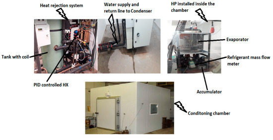
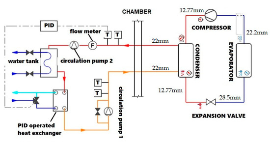
Figure 1.
Test facility with experimental setup in pictorial view with a schematic diagram.
Two circulation pumps were employed to maintain the required water flow rates inside the closed loop circuit. The second circulation pump works as a booster for achieving the higher water mass flow rates. The difference between the water supply temperature (WST) and entering water temperature (EWT), delta T, was controlled by PID-controlled heat exchanger on the load side. The water pipes with a 22 mm nominal diameter made of copper were used for the supply and entering water temperature across the condenser. The PID valve operated according to the supply temperature set points. The heat load was dumped to the water tank via the inserted coil and/or secondary heat exchanger by supplying fresh water from the water supply tank, fitted at the top of the roof. The testing procedure mentioned in BS EN14511-3 [14] was followed in terms of methodology, sensor, quantity, and measurement accuracy requirements.
2.2. The Control Devices and Data Acquisition System
The data logger instruments, measurement devices consisting of temperature, pressure, mass flow meters sensor, and control mechanism inside the chamber were properly chosen and installed to adequately perform the tests with good confidence in the testing results. All the measured variables were monitored, and data were recorded every 10 s with an average value considered for analysis purposes. The data utilized were obtained through recording and monitoring from (a) source side conditions, (b) inlet and outlet of the main components, and (c) load side quantities. On the source side, the ambient temperature and humidity were measured and controlled by the heater, cooler, and humidifier. The PID-controlled steamers were able to meet the requirements mentioned in the standard for the relative humidity (RH). The device types, measured quantity, and uncertainty associated with the measurement devices are shown in Table 2.
Table 2.
Uncertainties ranges for measurement instruments.
On the water side, the entering and supply temperatures were measured using a PT100 temperature sensor, the water mass flow rates were measured via a flow meter, and pressure gauges were used for pressure measurement. The pressure and temperature at the inlet and outlets of the compressor, condenser, evaporator, and expansion valve were subsequently measured. The refrigerant mass flow rate through the condenser and evaporator was measured through the flow meter installed in the liquid refrigerant line.
2.3. Experimental Procedure and Test Conditions
The ambient temperature, humidity, and WST values for the tested conditions, with definite constant heat loads, are shown in Table 3. The system performance was tested for the range of ambient temperature conditions at low (35 °C)-to-medium (45 °C) and high (55 °C) WST. The main testing regime was developed at a constant value of delta T of °C to make the result consistent and comparable because most of the existing buildings’ installed heat emitters were designed for a flow outlet/return temperature difference of 10 °C [43].
Table 3.
HP lab testing conditions.
2.4. Domestic Heat Load Demands for Irish Housing Stock
The tested HP system was designed and developed with an aim to meet domestic household heat load demand commonly required inside the Irish residential building for combined space heating (SH) and domestic hot water (DHW) demand. The heat load demands, including both the SH and DHW demand for five property types, were adapted from the experimental results [44], and are shown in Figure 2. The impact on the HP performance due to building type and age period, each of which has different insulations and thermal characteristics, is investigated by considering five property types with four age periods, making a total number of 20 archetypes, as reported in Table 4. The five property types of flats, mid-terraced, end-terraced, semi-detached, and detached with age periods of 1900–1949, 1950–1975, 1976–1990, and 1991–2007 onwards were considered in the analysis because a significant percentage (approximately 90%) of these housing stocks are present in Ireland, Northern Ireland, and Scotland [3,44].
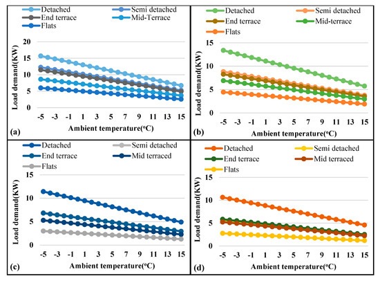
Figure 2.
Combined (SH and DHW) heat load demand for five property types and four age periods: (a) 1900–1949, (b) 19501975, (c) 1976–1990, and (d) 1991–2007 onwards.
Table 4.
The 20 buildings investigated according to building type and age period.
The average building load demand based on experimental results [44] was adapted for the five property types according to the age period duration. The building’s thermal characteristics during different age periods causes a load demand variation for the same property type due to different insulation characteristics and building standards during the considered period. Based on the results, the detached type represents the highest heat load demand during all age periods, while the flat type represents the lowest heat demand. The building space heat (SH) load demand was adapted for the considered property types using the building energy signature (BES) approach [42]. The heat load demand including both the SH and DHW demands in each bin is depicted in Figure 2.
The domestic hot water (DHW) demand weighted average value in percentage (%) demand was used according to the age period. The additional DHW percentage (%) shares of the annual SH demand considered were 15%, 16%, 18%, and 27% according to the four respective age periods of 1900–1949, 1950–1975, 1976–1990, and 1991–2007 onwards, respectively [5]. The hourly bin distribution depicted in Figure 3 for Belfast climatic conditions was retrieved from TRNSYS 17 Meteonorm weather file data [45].
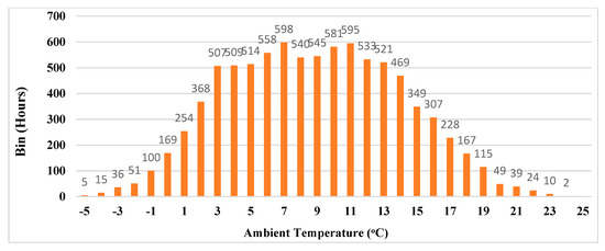
Figure 3.
Bin distribution for Belfast climatic conditions.
2.5. Mathematical Formulae
The HP coefficient of performance (COP) at each individual testing condition, defined as the ratio between the heat output and total electric power consumption, was calculated using Equation (1):
where is the heating capacity in kW, is the total electric power consumption in kW, is the water specific heat capacity, is the water mass flow rate (kg/s), and is the difference between the water supply temperature (WST) and entering water temperature (EWT).
The compressor isentropic efficiency, defined as the ratio between the isentropic thermodynamic work and the actual thermodynamic compressor work, was calculated by Equation (2):
The volumetric efficiency of compressor, or the ratio between the actual mass flow rates at the compressor suction and the theoretical value of the mass flow rates, was calculated by Equation (3):
where and represent the respective refrigerant specific volume and mass flow rates at the compressor suction, respectively, and denotes the compressor speed. Experimental work has an associated uncertainty to a certain extent based on the independent variables measured, contributing to the error of the final experimental results. The error associated with the individual measuring devices mentioned in the methodology was utilized to find the total error for the heating capacity, electric power consumption, and COP. The error analysis was performed using the approach developed by the ASHRAE guidelines [46] with the following equations.
The percentage error for every quantity varies according to the measured values, with the heating capacity variation ranges from minimum value of ±4.61% to a maximum value of ±21.12% for the tested heating capacity range. The electric power was measured with ±1.5% accuracy, and the error associated with the COP was in the range of ±0.26% to ±6.98%.
The bin method was used for the evaluation of the annual performance for the five property types. The COP in each bin after correction factor multiplication, and the electrical energy consumption (E) for the heat pump only, were calculated by Equations (6) and (7), respectively.
The in Equation (8) determines the COP correction factor.
2.5.1. Model Validation with Testing Results
The HP numerical model was developed and calibrated at nominal heating capacity testing results using the approach suggested by other researchers [37,47] for the parameter identifications. First, the model was calibrated with nominal heating capacity tests for finding the coefficient values, followed by the model validation with other testing results. The developed numerical model consisted of two outputs— the coefficient of performance (COP) and electric power consumption (P) determined by Equations (9) and (10), respectively.
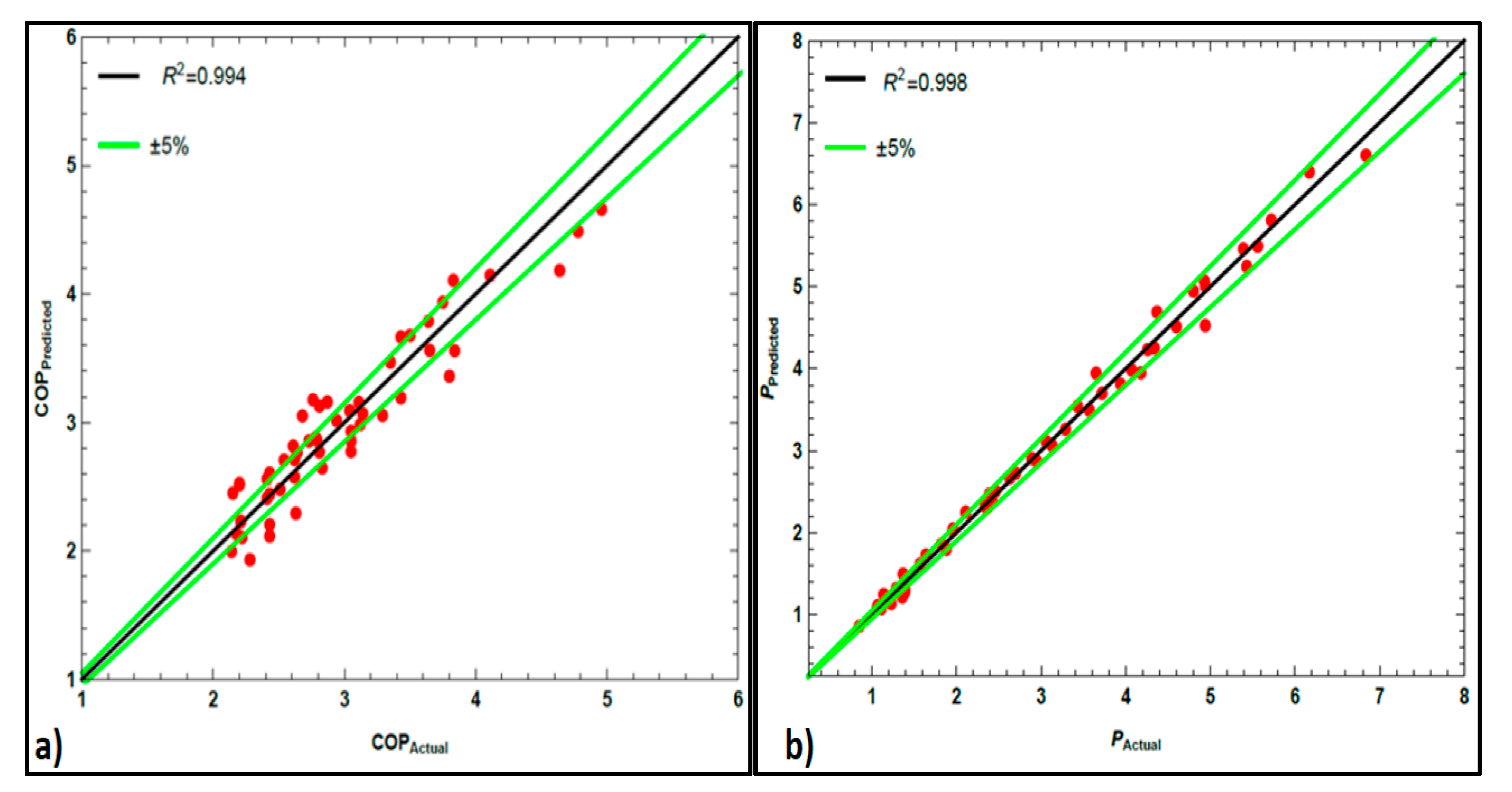
The outputs of the model were dependent on three variables, i.e., the water supply temperature (WST), ambient temperature conditions, and operating speed. The model calibration and validation shown in Figure 4 was performed with experimental test results using the Mathematica software [48]. The comparison was conducted between the measured experimental and predicted values to have an idea of the model error via the root-mean-square error (RMSEs) approach, defined by Equation (11).
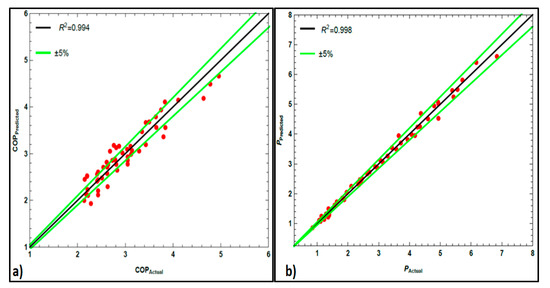
Figure 4.
HP model validation with experiments (a) COP (-) and (b) power, P (Kw).
2.5.2. HP Part Load Performance
The HP part load performance in different property types with varying loads in each bin during the VSM of operation and FSM of operation were evaluated using Equations (12)–(14), with the same the approach developed by other researchers [49,50,51,52].
The annual COP, or the ratio between the total useful heat output divided by the total electric power consumption for the complete year, was calculated by Equation (15).
The total electric power consumption (P) was the combination of the HP electrical energy plus the back-up electrical energy consumptions.
3. Results Analysis and Discussions
3.1. HP Testing Results at Low-to-Medium and High Heat Supply Temperature
The HP testing results with heating capacity range of 3–18 KW, at the low (35 °C)-to-medium (45 °C) and high heat supply temperatures (55 °C) required for the underfloor, DHW, and radiator heating distribution systems are presented and discussed. Table 5, Table 6 and Table 7 show the summary results at low-to-medium and high heat supply temperatures, respectively.
Table 5.
Heat Pump test results summary at the lower heat supply temperature of 35 °C.
Table 6.
Heat pump test result summary at the medium heatsupply temperature of 45 °C.
Table 7.
Heat pump test result summary at the high heat supply temperature of 55 °C.
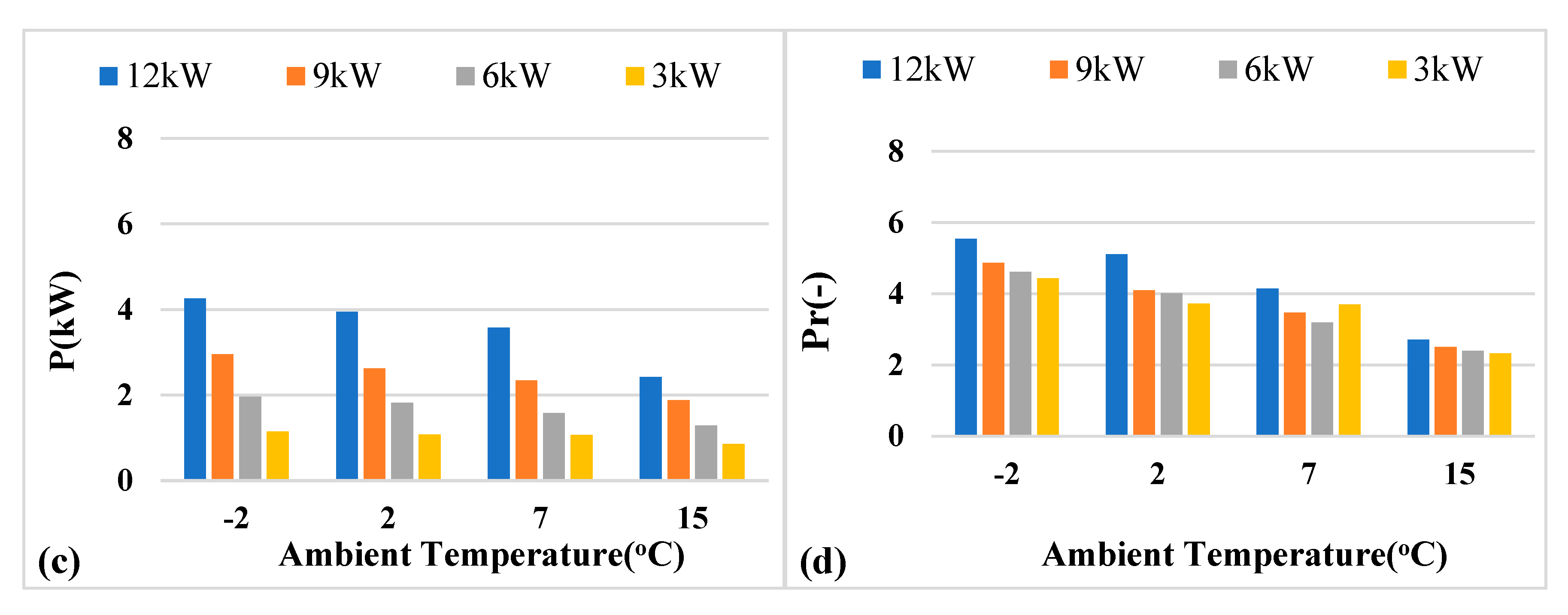
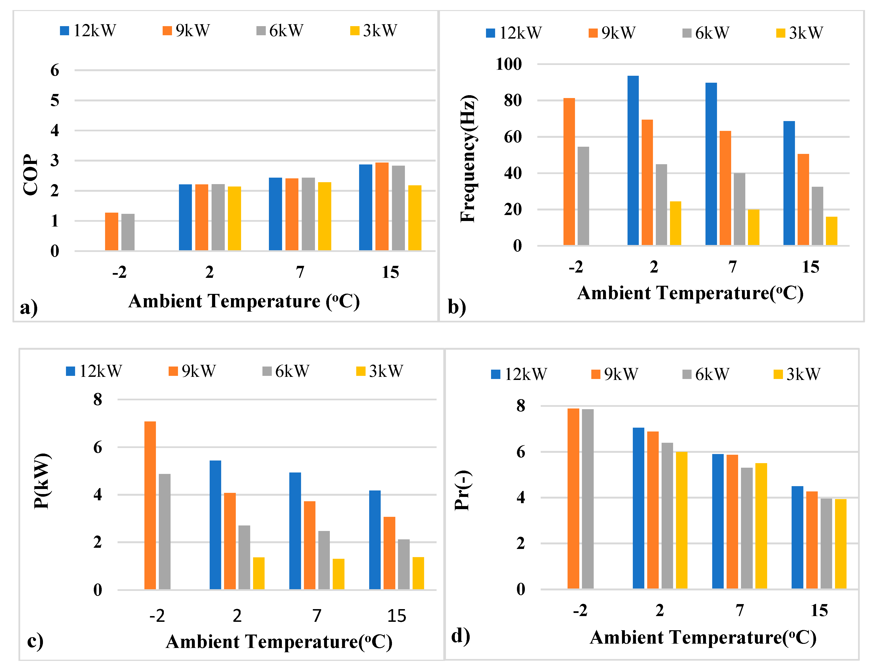
The impact of low-to-medium and high heat supply temperatures on the (a) COP, (b) frequency (Hz), (c) power consumptions, and (d) pressure ratio is shown in Figure 5, Figure 6 and Figure 7, respectively. The tested fixed heating capacity with varying water mass flow rates inside the closed loop circuit, COP values, compressor volumetric and isentropic efficiencies, inverter losses as a percentage of the total power consumption, discharge line temperatures (DLTs), and pressure ratios showed significant variation due to heat supply temperature. The overall performance improved with the lower heat supply temperature because of the lower pressure ratio, discharge temperature, and improved compressor efficiencies. At the fixed heat supply temperature, the ambient temperature conditions at the nominal speed operation at all tested conditions showed superior performance than the low and upper speed operations than that of the nominal speed value. The reason for this was the high compressor isentropic and volumetric efficiencies, and the lower inverter losses, pressure ratios, and discharge line temperature. The system works at a wide range of changing pressure ratios between the high-pressure condenser side and lower pressure evaporator side, and only at a single nominal operating point was the cycle external pressure ratio equal to that of the compressor internal pressure ratio. The linear degradation of the volumetric efficiencies was observed with the decreasing pressure ratio for all tested conditions below and above the nominal speed value. The compressor isentropic efficiency, volumetric efficiency, pressure ratio, inverter losses, and electric power consumption contribute to the overall system performance and COP values. The compressor work and electrical energy requirements increase with the increase of speed of operation because the system is working on a higher amount of the refrigerant mass flow rate per volumetric displacement of the compressor. The inverter losses as a percentage of the total electric power consumption are increased at lower heating capacities due to its poor performance at low-speed operation. The steady state test results show the impact of the compressor efficiencies due to speed variation and inverter losses.
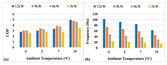

Figure 5.
(a) COP, (b) frequency (Hz) values, (c) power consumption, and (d) pressure ratio for the fixed heating capacities at the heat supply temperature of 35 °C.
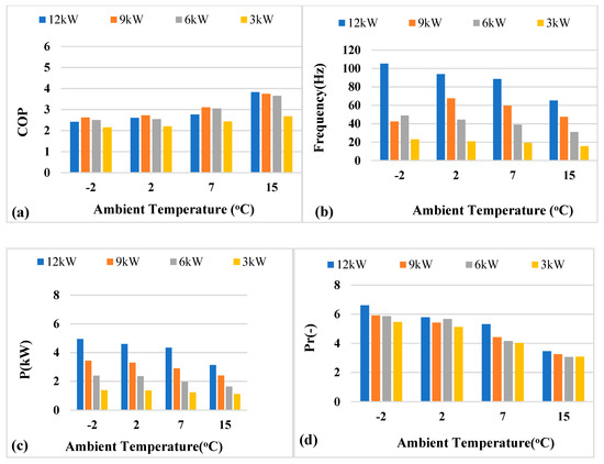
Figure 6.
(a) COP, (b) frequency (Hz) values, (c) power consumption, and (d) pressure ratio for the fixed heating capacities at the heat supply temperature of 45 °C.

Figure 7.
(a) COP, (b) frequency (Hz) values, (c) power consumption, and (d) pressure ratio for the fixed heating capacities at the heat supply temperature of 55 °C.
The tested results were used to model the HP for the annual COP evaluation into different property types. The system annual performance simulated against the heat load demand in two control modes (VSM and FSM) and at three heat supply temperatures, considered here as C1, C2, and C3, which are presented in the following sub-sections for the different property types. The COP values vary according to the part load operation, heat supply temperature, and control mode. The role of transient losses becomes very crucial while comparing the control mode for the capacity control for different heat load demands in the evaluation of the annual performance. In the following sections (Section 3.2, Section 3.3, Section 3.4, and Section 3.5) the part load performance, difference in power consumptions and heating production, annual performance, and respective payback period analysis for the single age period of 1900–1949 are discussed in more detail for the five property types. This is summarized and extended to all age period in Section 3.6.
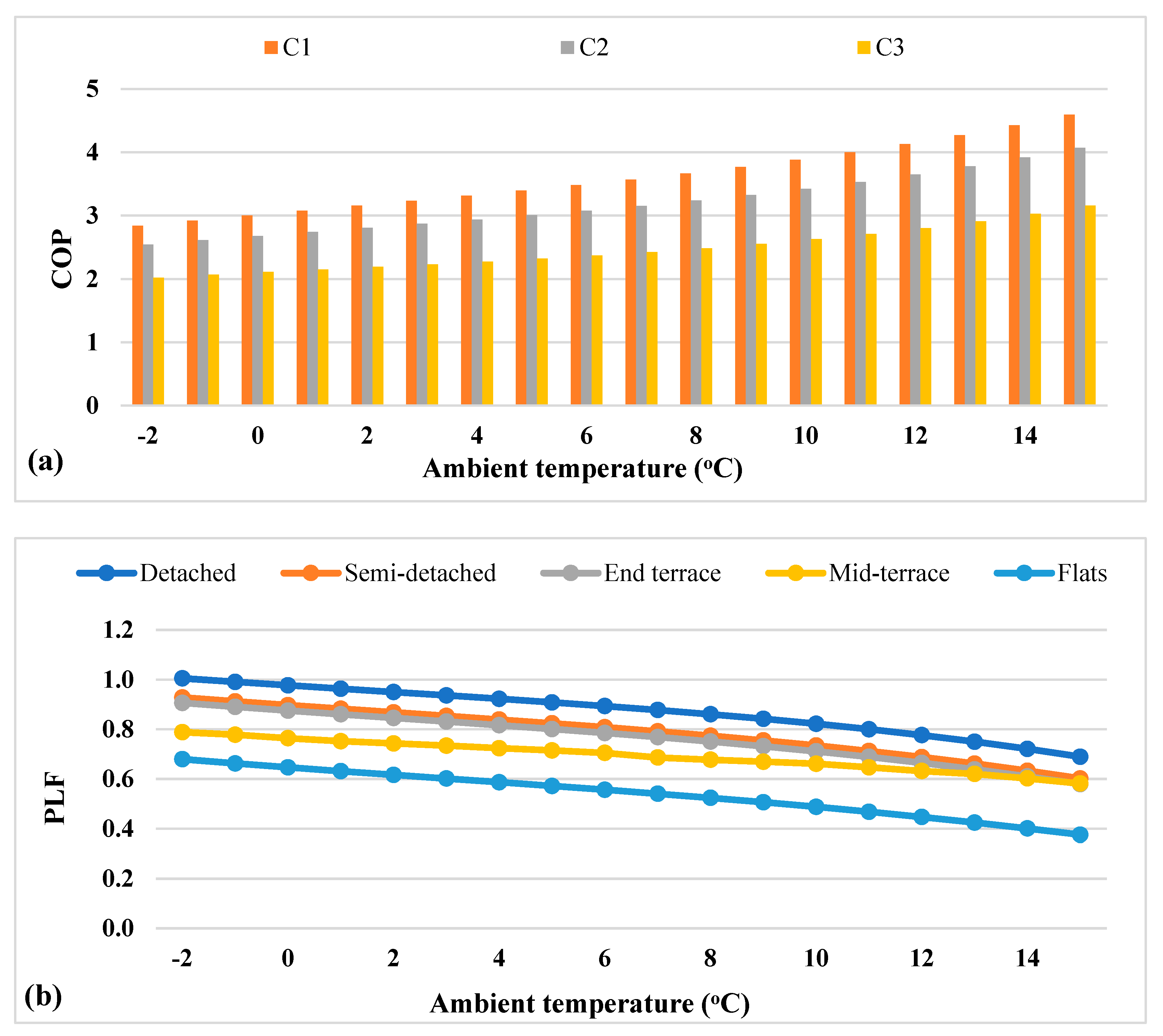
3.2. Part Load Performance for the Five Property Types with a Single Age Period (1900–1949)
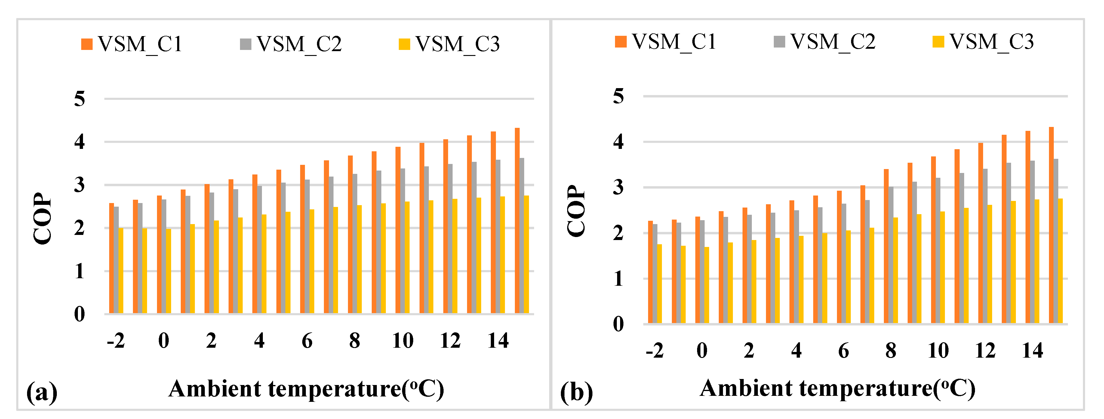
The model was used for the system performance prediction for five different property types in two control modes of operation (VSM and FSM). The HP meets the heat load demand across the experienced ambient temperature conditions in the VSM of control for all five property types by adjusting the heating capacities via the compressor speed. Keeping balance between the house heat loss and HP heat capacity means maintaining the thermostat temperature at a set point, using a fully controlled system resulting in higher thermal comfort. The thermal heat load demands for each property type influences the HP performance in each bin. The part load performance with VSM in each bin for the five property types over the experienced ambient temperature conditions, at three heat supply temperatures, is shown in Figure 8, Figure 9, Figure 10, Figure 11 and Figure 12. The COP values with detached type, representing the highest heat load demand (Figure 8) at high ambient temperature conditions, are higher compared to other property types because of the part load factor and the continuous compressor operation near to the nominal speed values. In the case of the flat type, representing the lowest heat demand, the COP values at a higher ambient temperature degrade due to lower speed operation and additional cycling losses. At the lowest ambient temperature conditions of −2 °C, the detached-type building causes lower COP values due to an inefficient compressor operation at full speed, while the other property types of semi-detached, end-terraced, mid-terraced and flat type show a COP improvement due to the near compressor operation at nominal speed. Transient losses associated with the system are mainly due to cycling losses and the defrost strategy. During VSM, the overall system efficiency is improved by continuous operation due to a match between the heat load demand and heat supplied over the full range of experienced ambient temperature conditions for the five property types without or with very rare cycling losses. The main issue is the frosting effect occurring at the surface of the evaporator at low ambient temperatures and high relative humidity due to air flow rate reduction, which causes a low evaporating temperature and pressure, resulting in poor performance (COP), a higher electrical energy consumption, and an increased compressor pressure ratio. The COP values before and after the experimentally established frosting effect considerations are depicted.

Figure 8.
Detached type in VSM (a) without and (b) with considering defrost.
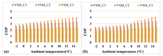
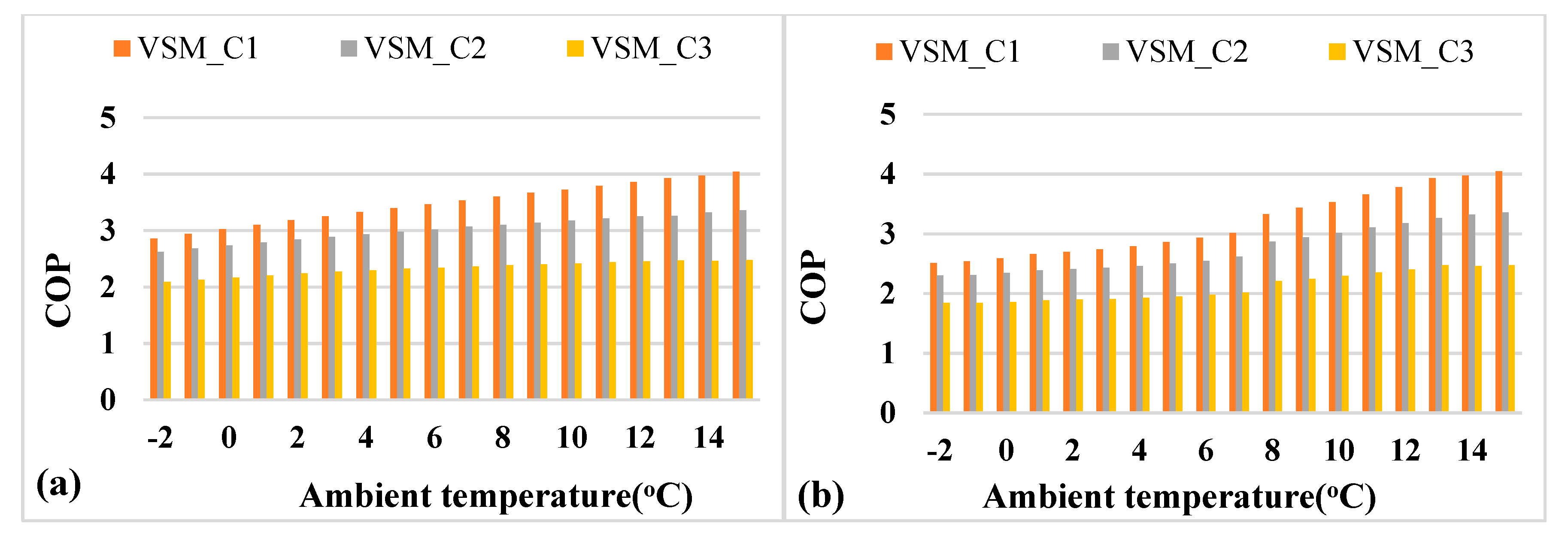
Figure 9.
Semi-detached type (a) without and (b) with considering defrost.
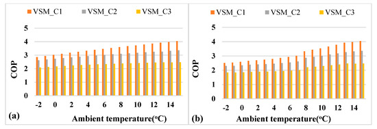
Figure 10.
End-terraced (a) without and (b) with considering defrost.
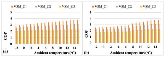
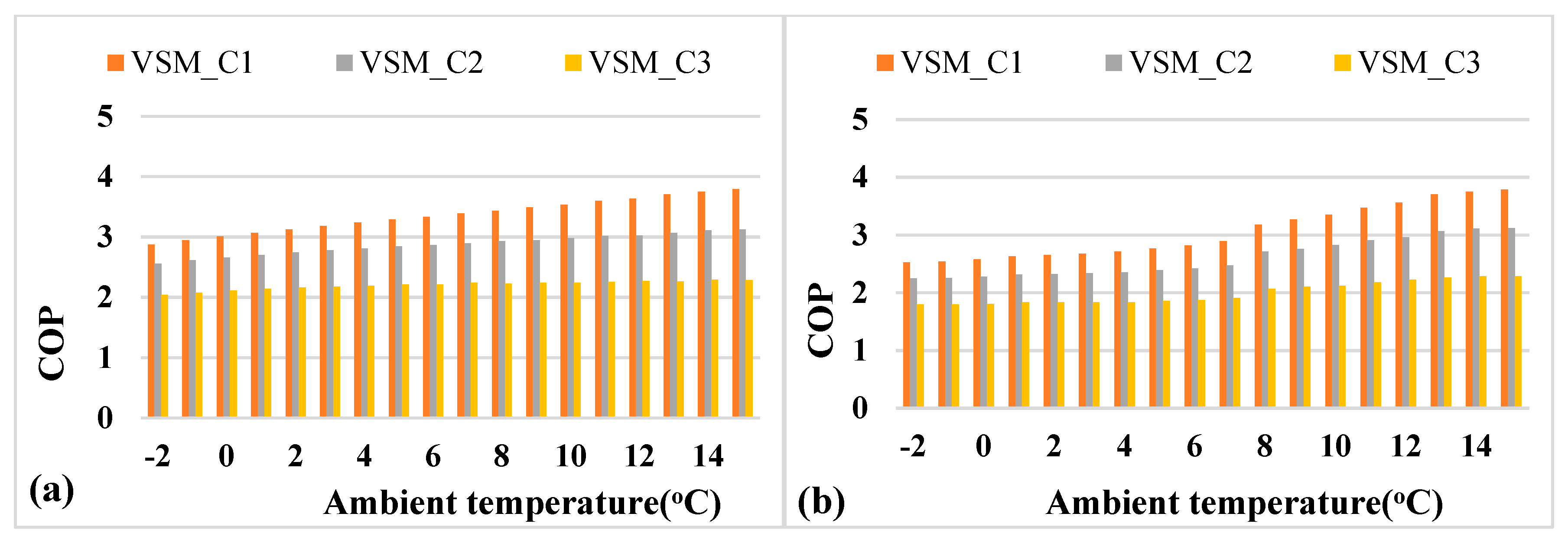
Figure 11.
Mid-terraced (a) without and (b) with considering defrost.
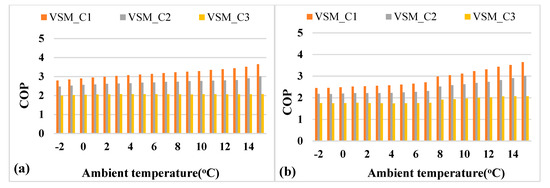
Figure 12.
Flat type (a) without and (b) with considering defrost.
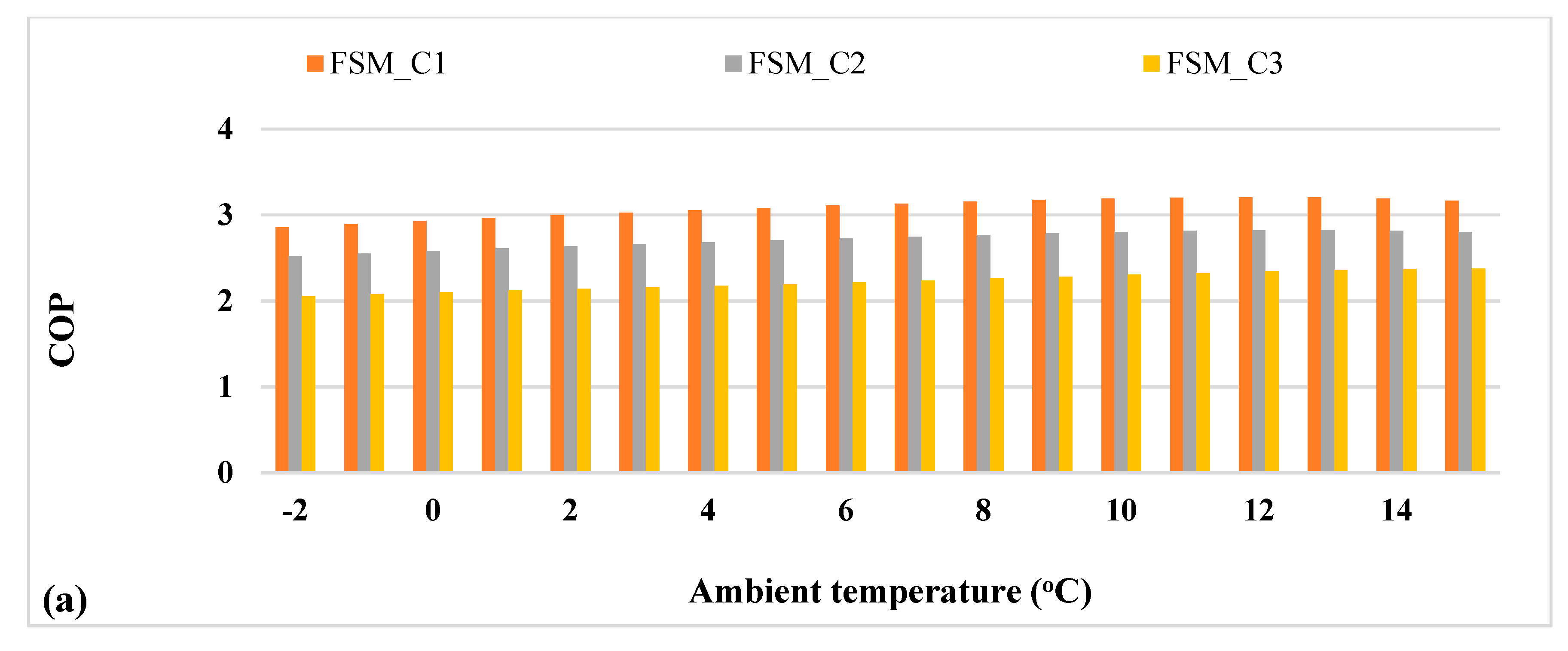
Figure 13a shows COP values for the three cases (C1, C2, C3) without considering the transient losses in each bin during FSM. The COP values are at the maximum in each bin due to nominal speed of operation. However, the maximum COP in each bin would not help in favor of the fixed speed operation for the system, as it causes over and under heat production in case of the respective operations from above and below to that of balance point. The overproduction causes an overshoot of the room temperature, resulting in cycling losses and lower production causes the back-up electrical heater requirements, and both of these impact the network stability at large-scale installations of such systems. The system operation in FSM at the maximum COP was possible at the nominal value, but without matching the heat load values and required on/off cycles for the capacity control, resulting in cycling losses. The intermittent operation has a negative impact on the compressor durability and thermostat overshoot and undershoot issues. The correction factor (CF) for the five property types considering the transient losses is shown in Figure 13b. The CF depends upon the thermal load demand and part load operation for the individual property type. Figure 14a–e shows the COP values for all five property types when the part load operation with cycling losses was considered.
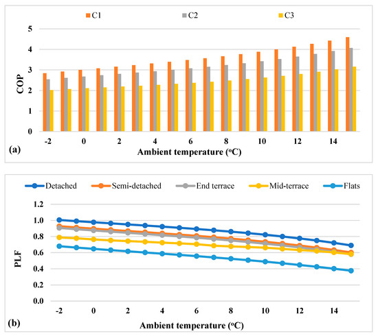
Figure 13.
FSM operation: (a) COP values without considering cycling losses and (b) correction factor for all five property types according to thermal load demand.

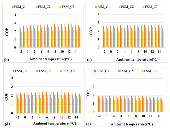
Figure 14.
COP values after correction factor: (a) detached type, (b) semi-detached type, (c) end-terraced type, (d) mid-terraced type, and (e) flat type.
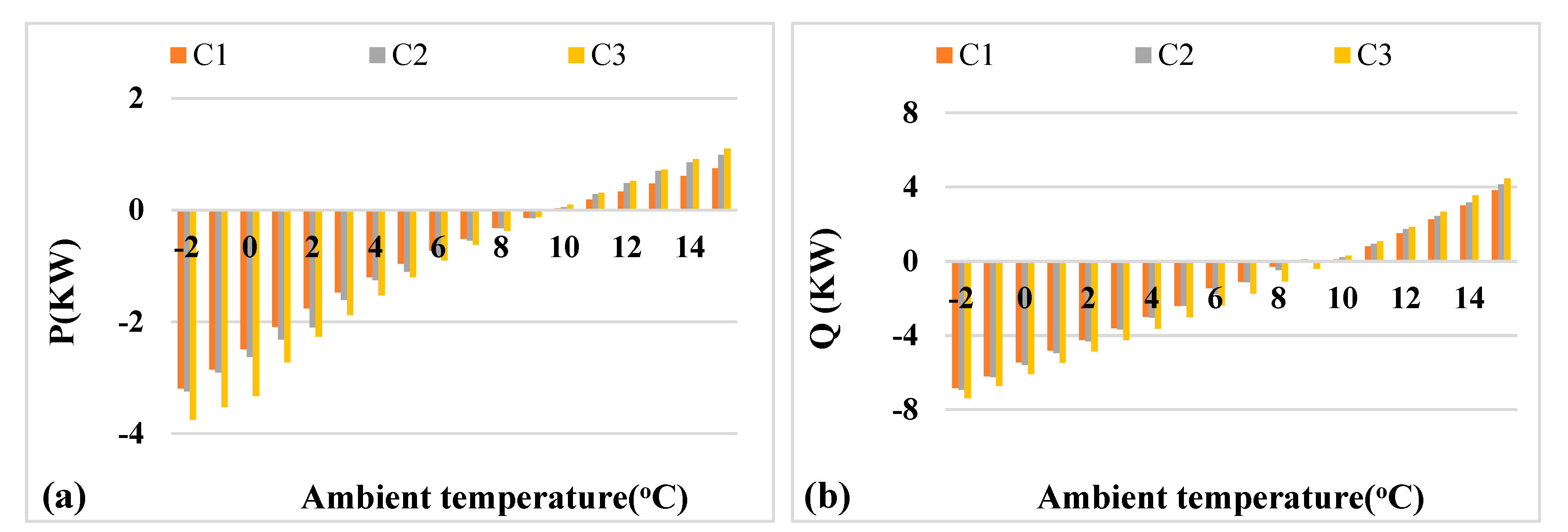
3.3. Electric Power Consumption and Heating Production Difference (FSM vs. VSM)
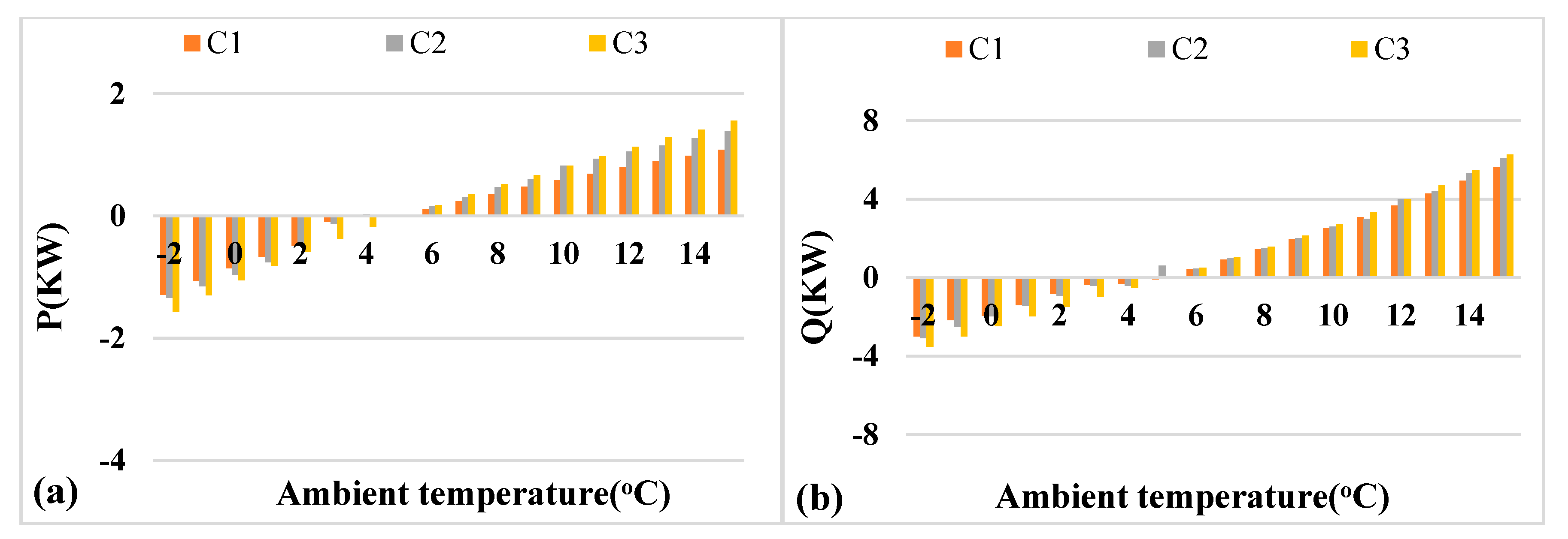
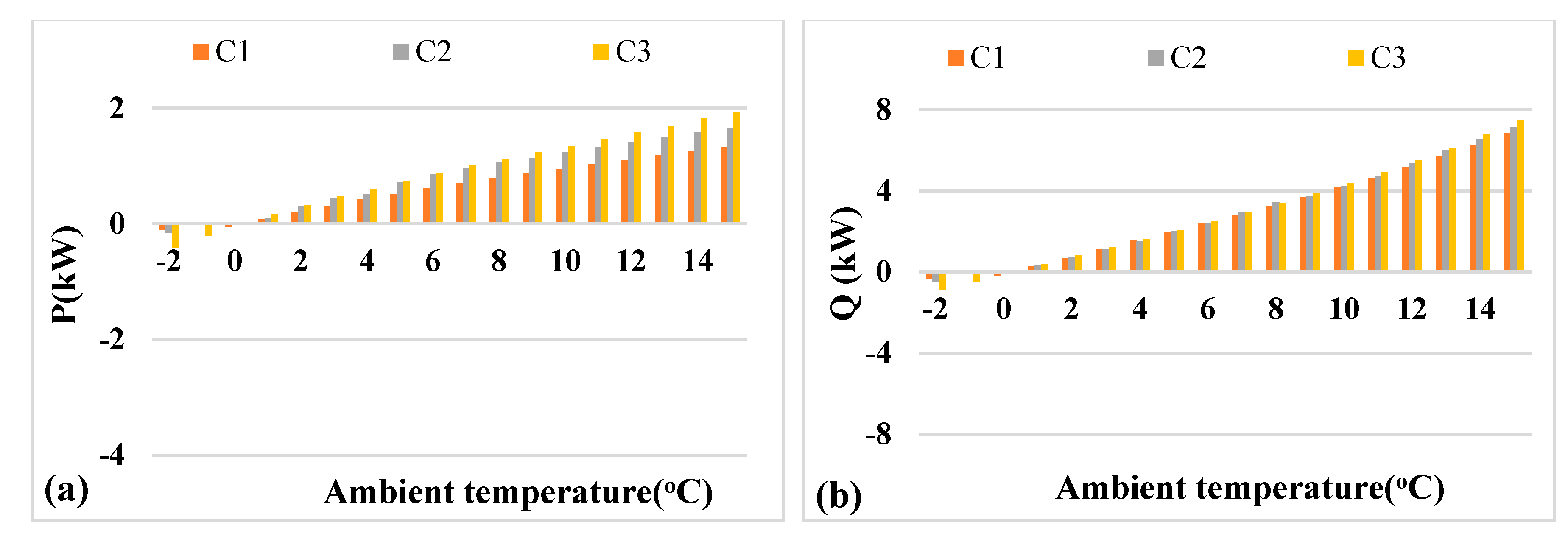
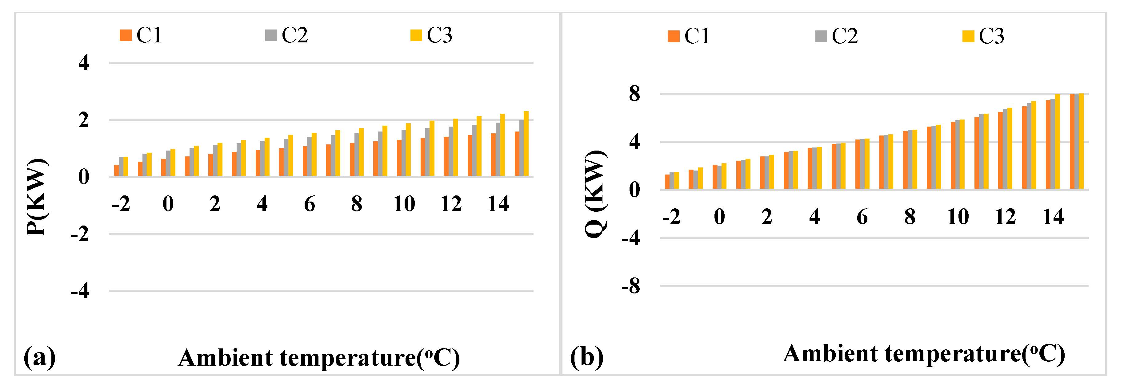
The comfort level and network stability are higher in the case of VSM because of the good match between the load demand and supplied energy. However, the thermal comfort and network stability could not be the only criteria for choosing the VSM operation over the FSM of control, as the poor performance may result in higher energy consumption and carbon emissions. The operating mode selection needs to be prioritized in terms of performance as well, and the VSM could be given preference when the cycling losses with the FSM at the maximum COP are large enough, degrading the system’s overall performance. The difference in electric power consumption and heating capacity for VSM vs. FSM for the five property types are shown in Figure 15, Figure 16, Figure 17, Figure 18 and Figure 19. The additional heating capacity production causes the fluctuation in temperature control inside the built environment on the customer side. The network instability on the grid side is also caused by the intermittent operation and higher power requirements, resulting in grid frequency fluctuation. The additional heat produced causes reduction in on the on-cycle duration and an increase in the off-cycle. The thermostat temperature overshoot because of the increased heating capacity at higher ambient temperatures is one of the main issues, specifically with the underfloor heating distribution system (35 °C) that have thermal lag due to high thermal inertia [14,15]. On the other hand, thermostat temperature undershoots become a problem at very low ambient temperatures when the HP heating capacity reduces with the low heat supply temperature. The balance point has an impact on the overall annual COP for different property types. In the case of the detached type, with the HP with the FSM of control, the heat production was lower than the required heat load below the balance point of 9 °C. The back-up electric heating becomes essential for meeting the heat load in the range of −2 to 9 °C, resulting in a lower overall annual COP. In the case of the semi-detached-type building, the back-up electric requirements start with a balance point of 6 °C and subsequently reduce to 5 °C and 0 °C in the case of end-terraced and mid-terraced buildings, respectively. In the case of the flats type, additional heat is produced over the full range of experienced ambient temperature conditions.
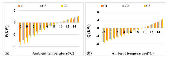
Figure 15.
HP difference (VSM vs. FSM) for Detached type in (a) Power (P), (b) Heating capacity.

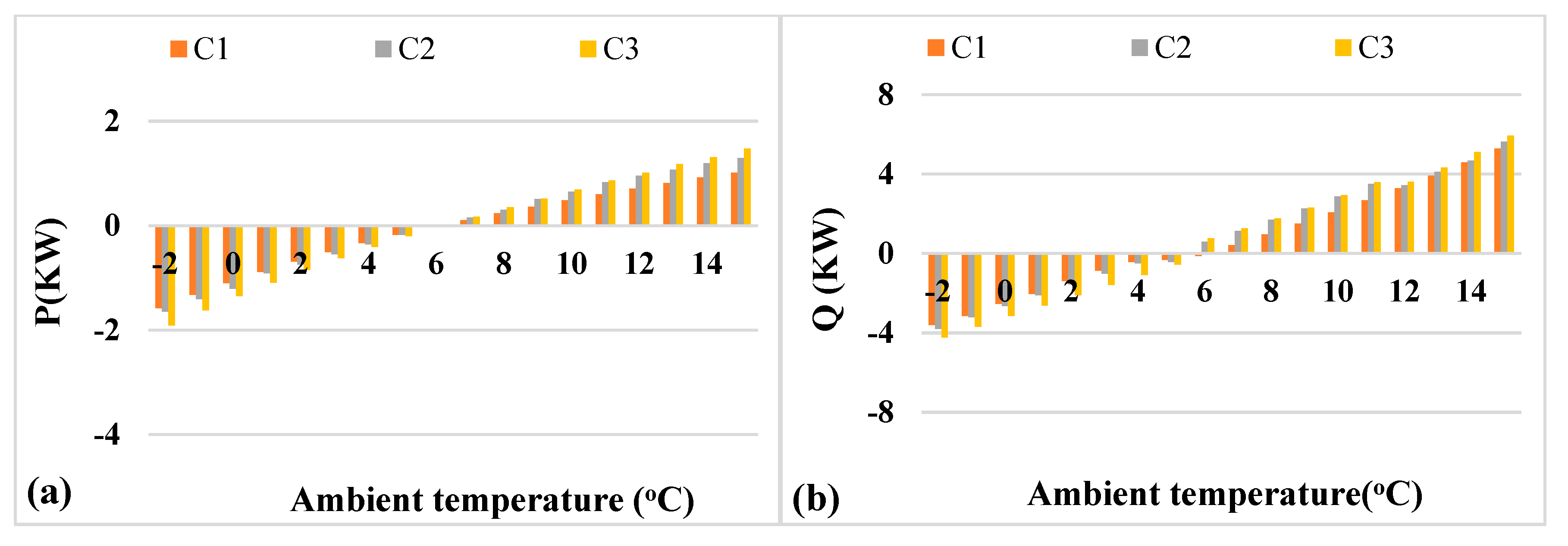
Figure 16.
HP difference (VSM vs. FSM) for semi-detached type in (a) power (P) and (b) heating capacity (Q).

Figure 17.
HP difference (VSM vs. FSM) for end-terraced type in (a) power (P) and (b) heating capacity.
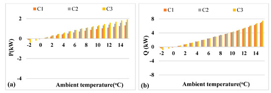
Figure 18.
HP difference (VSM vs. FSM) for mid-terraced type in (a) power (P) and (b) heating capacity.
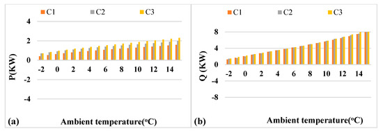
Figure 19.
HP difference (VSM vs. FSM) for flat type in (a) power (P) and (b) heating capacity.
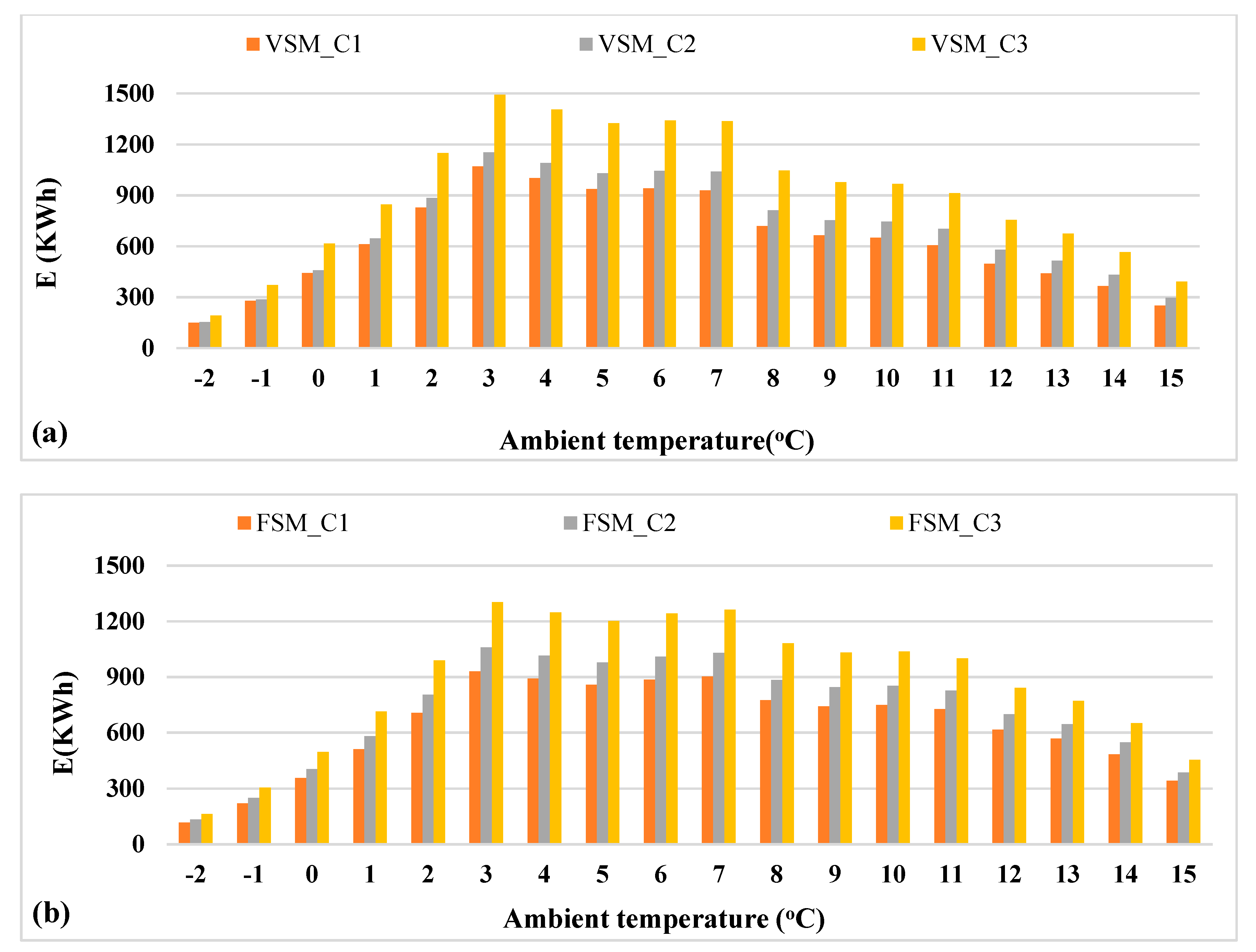
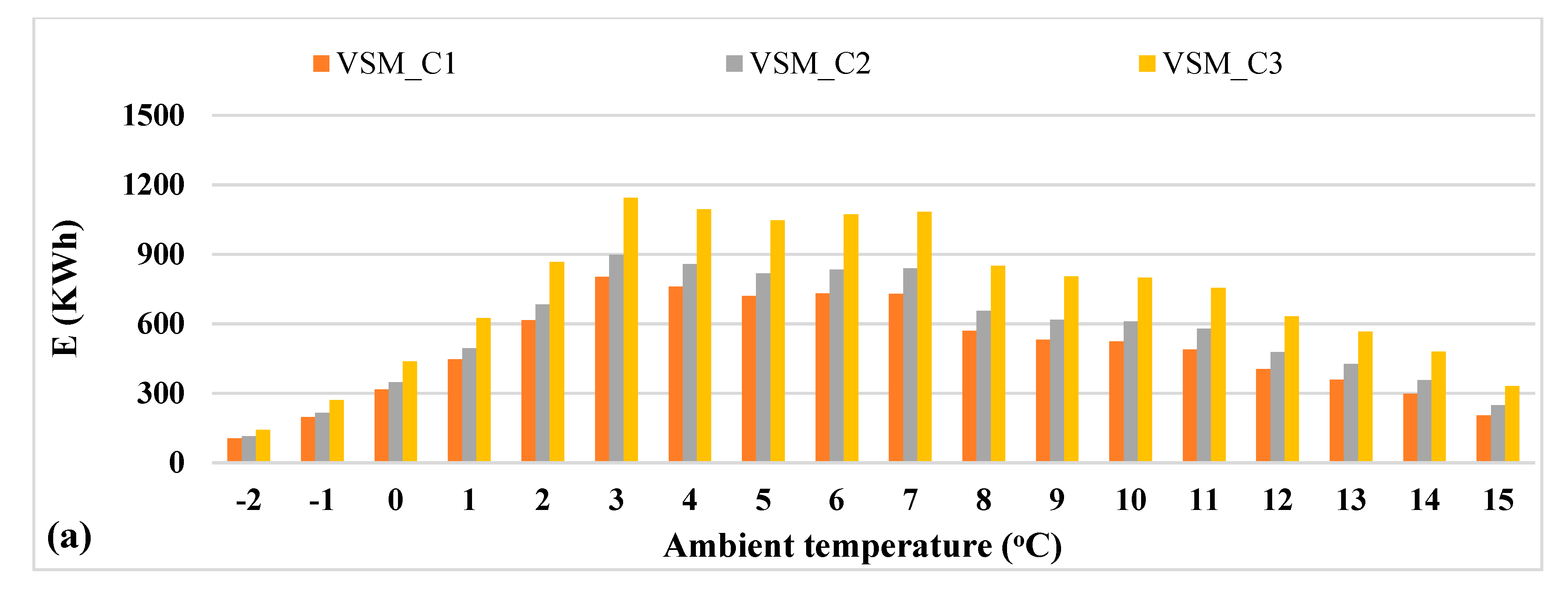
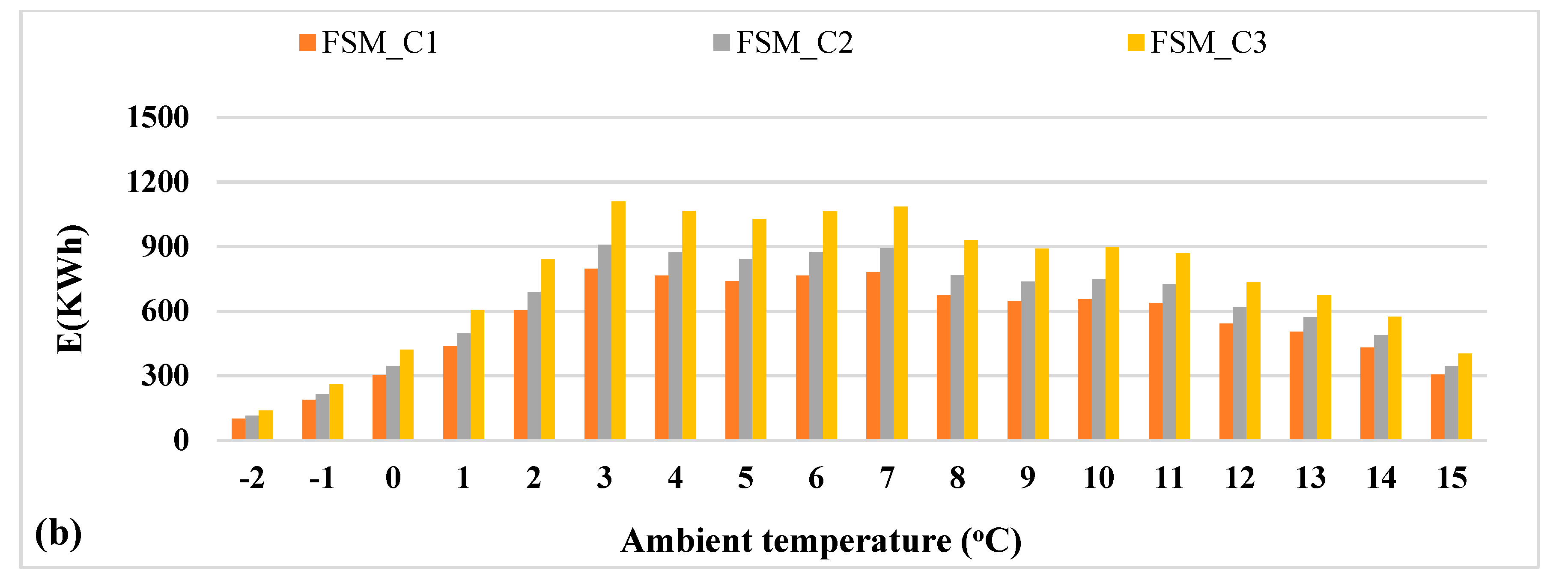
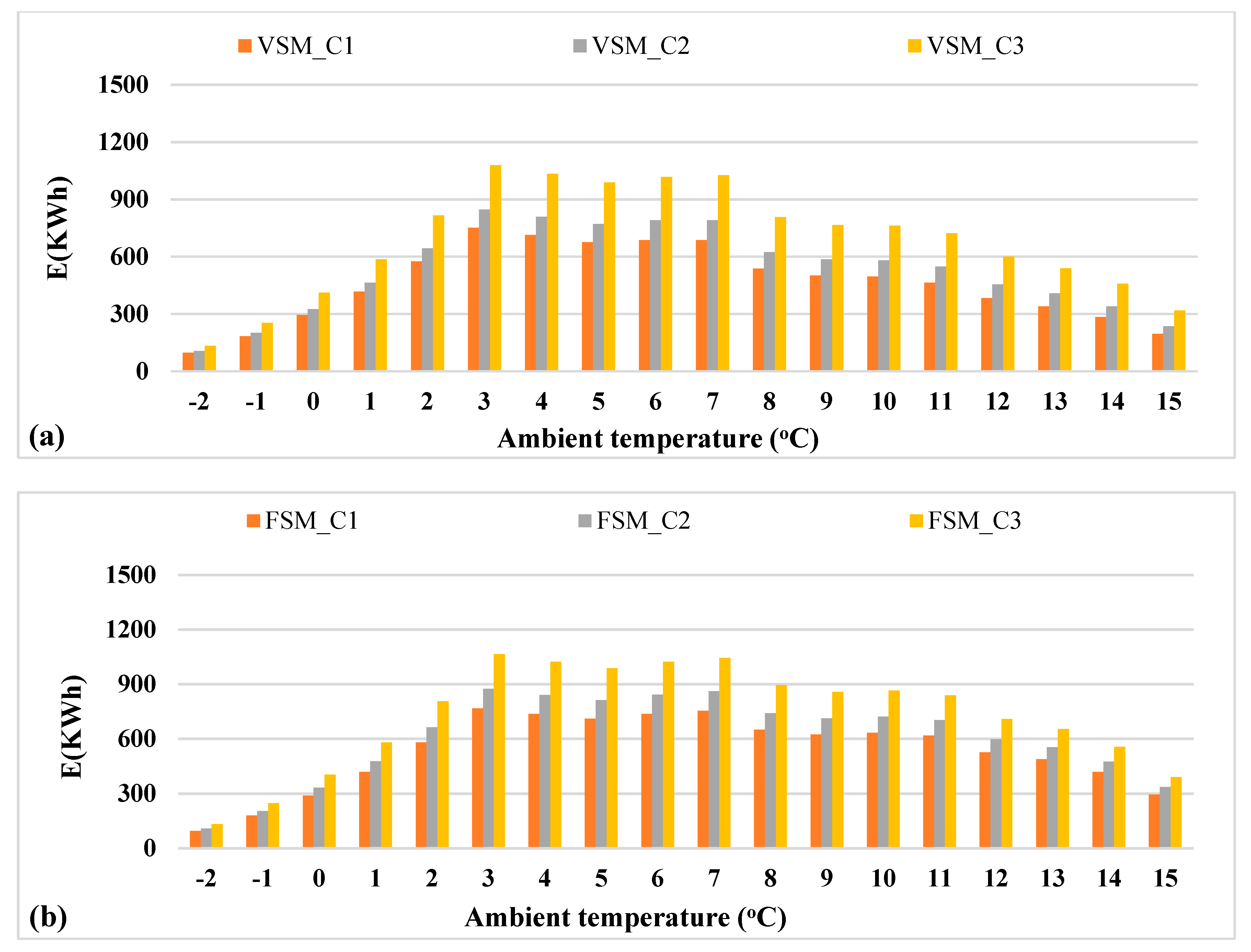
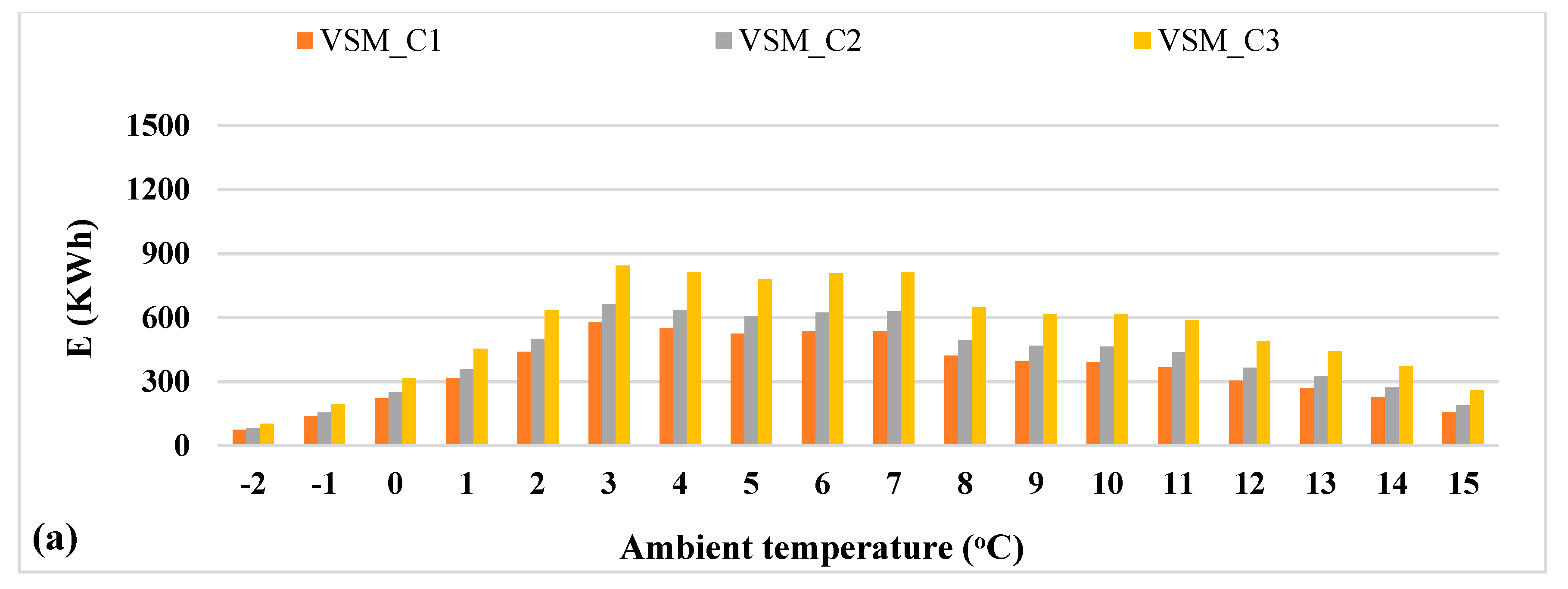
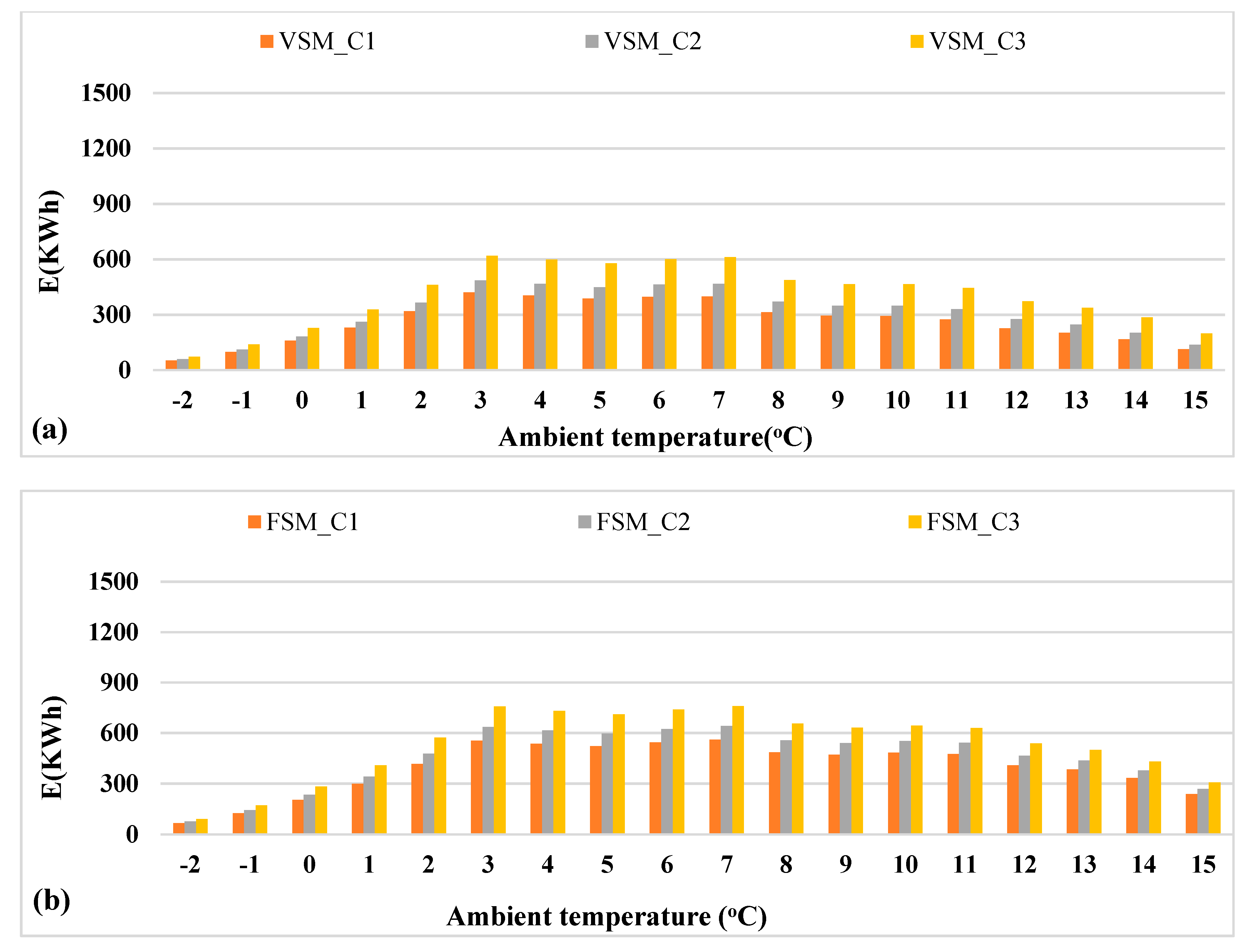
The annual heat load demand for all five property types in each bin is shown in Figure 20. The flat type represents the lowest heat demand in all bins and the detached-type building represents the highest load demand. The 7 °C temperature occurs for the most hours during the complete year, resulting in the highest heat load demand for the Belfast climatic conditions. The property type with balance points closer to the 7 °C in Belfast climatic conditions would have an even better performance, even during FSM. The corresponding required electrical energy consumption for the HP (FSM and VSM) for the five property types in each bin is shown in Figure 21, Figure 22, Figure 23, Figure 24 and Figure 25. In the case of FSM where HP is unable to meet the required load demand at lower ambient temperatures, the back-up electric heater was utilized. This also results in the higher HP energy consumptions in VSM compared to FSM. However, it should be noted that the heating demand in FSM is assisted by back-up electric heater requirements in this scenario, resulting in a lower overall COP [22]. This is the case for the detached and semi-detached property types (Figure 21 and Figure 22), when the HP in FSM is unable to meet the required load demand in each bin, which causes annual back-up electrical energy consumptions of 5333 KWh and 1516 KWh, respectively, for the property types (Table 8). The back-up electric demand in FSM subsequently reduces when the HP is capable of meeting the full load demand.
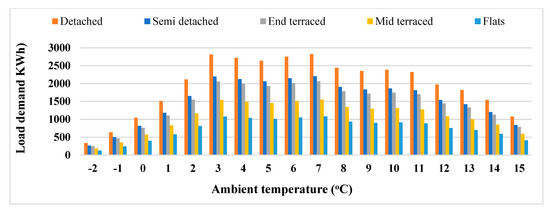
Figure 20.
Annual heat load demand (KWh) for all property types in each bin.
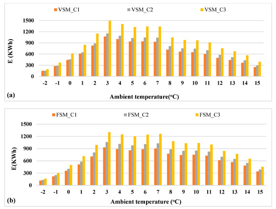
Figure 21.
Detached type annual electrical energy consumption (E) with (a) VSM and (b) FSM.
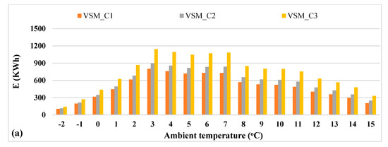
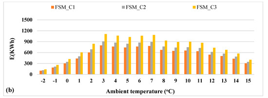
Figure 22.
Semi-detached type annual electrical energy consumption (E) with (a) VSM and (b) FSM.
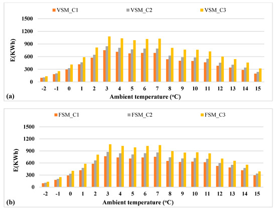
Figure 23.
End-terraced type annual electrical energy consumption (E) with (a) VSM and (b) FSM.

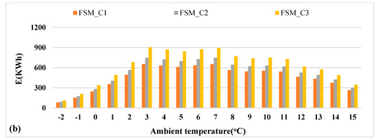
Figure 24.
Mid-terraced type annual electrical energy consumption (E) with (a) VSM and (b) FSM.

Figure 25.
Flat type annual electrical energy consumption (E) with (a) VSM and (b) FSM.
Table 8.
HP annual performance in different property types.
3.4. Annual Performance for Five Property Types (1900–1949)
The summary results for the overall annual COP, HP useful annual heat output, electrical energy demand in two modes of operation, the three cases (C1, C2, C3) considered, and the back-up electric heater contributions for the five property types are presented in Table 8. The annual COP depends on the annual building load demand, considering the case based on the heat supply temperature level (C1, C2, C3), back-up electric heater (EH) requirements, and the operating mode of control.
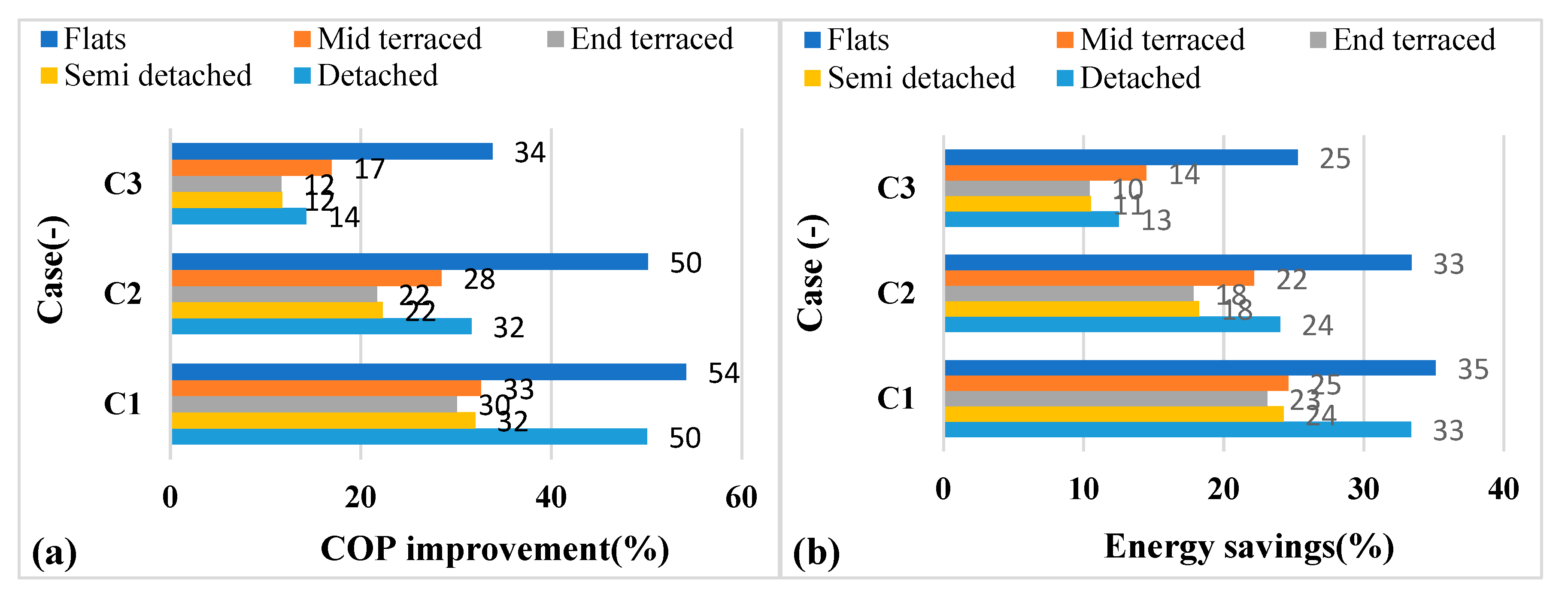
The annual COP improvement and energy savings due to the operating mode of control (VSM vs. FSM), and the heat supply temperature (C1 vs. C3) with different percentages for all property types depending on part load factor, are shown in Figure 26 and Figure 27, respectively. The COP improves and energy savings are increased with a lower heat supply in comparison to a higher heat supply temperature for both control modes, but with different percentage values. The COP improvement and energy savings due to the heat supply temperature during VSM are higher for all property types in comparison to the FSM. It could be concluded that the variable speed operation at a lower heat supply temperature is more beneficial in comparison to a high heat supply temperature. The annual COP during FSM is at the maximum with a value of 2.27 for the semi-detached type due to balance point match and the maximum number of hours of operation for Belfast Climatic conditions at 7 °C. The back-up electric heater requirements are the highest for the detached-type building with a demand of 5333 KWh during the FSM. However, the highest back-up electric heat demand is among the reasons for the poor overall performance, with the main issue of cycling losses.
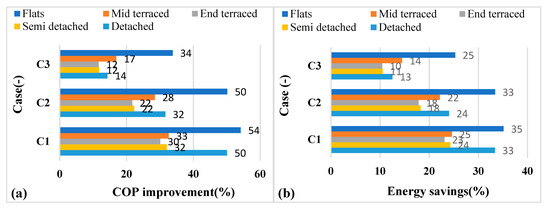
Figure 26.
VSM vs. FSM for the annual (a) COP improvement (%) and (b) energy savings (%).
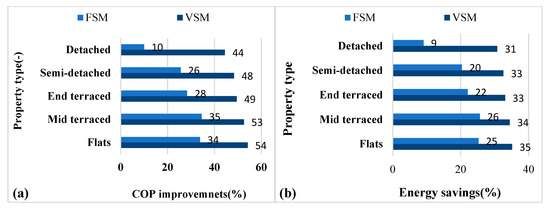
Figure 27.
C1 vs. C3 for the improvement in (a) COP and (b) energy savings (%).
3.5. Payback Period Analysis
The payback period analysis for VSM and low temperature heating distribution installations is summarized in Table 9. The annual running cost savings with the HP operation depends on the control mode of operations and the installed heating distribution systems. The additional cost associated with VSM in contrast to the FSM is calculated as 1000 GBP [53], with the payback period depending on the case considered. The HP at low heat supply temperature of 35 °C needs an additional installation cost of GBP 6000 [54], and the payback period was found as 10.2 years in FSM and reduced to 9 years in the case of VSM. The cost analysis in the present calculation uses the simple payback period approach by Equation (16).
Table 9.
Payback period for control modes (VSM vs. FSM) and cases (C1 vs. C3).
3.6. Summary Result for Five Property Types with Four Age Periods
Table 10 summarizes the HP annual useful heat output, COPs, and electric energy consumption for the five property types, in two control modes, three cases, and four age period for the Belfast region. The heat demand depends on the property type and age period, and increases for the older age period due to poor insulation properties and lower thermal inertia.
Table 10.
HP performance in different property types and age periods.
Among the five property types considered, flats represented the lowest annual heat demand, ranging from 14,564 KWh to 6670 KWh, with the detached type representing the highest annual heat demand in the range of 38,085 KWh to 25,807 KWh, with the corresponding age period with the maximum demand being the old age period (1900–1949).
3.6.1. Annual COPs
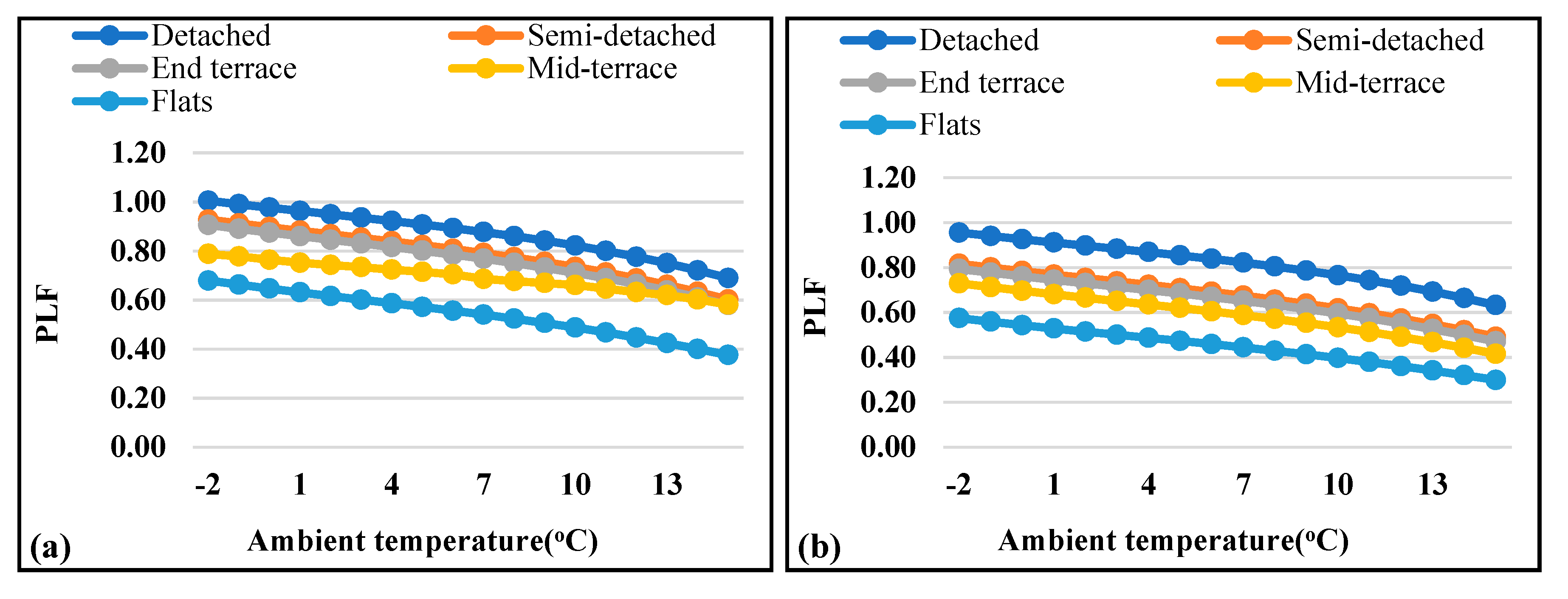
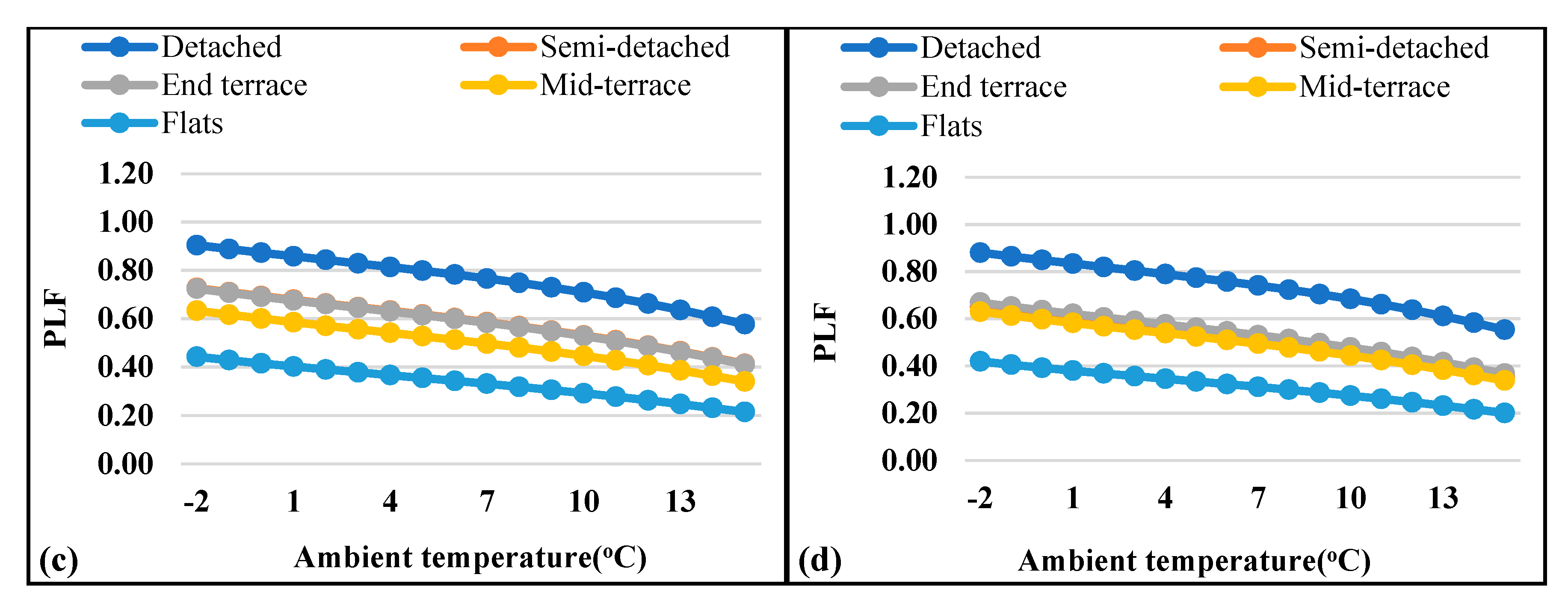
The HP annual COP for the different property types depends on the HP operating capacity, part load ratio, and the mode of control. The COP relation with the heat demand variation due to age factors for all five property types was not linear, but rather depended on the HP heating capacity match to the load demand in each bin and part load factor. The HP proved to be the least efficient in the flat type for all age periods compared to other types, and this was because of higher losses and lower part load operations. The flat type of the old age period (1900–1949) represented the highest COP. The part load factor with different load demands according to the age period for all five property types is depicted in Figure 28. The overall annual COP trend in VSM showed an increase with the increase of building heat demand for four of the property types (flats, mid-terraced, end-terraced, semi-detached), and was reduced for the detached types due to the operating point for the HP. The age factor effects the COP values for the specific case studied and the control mode.
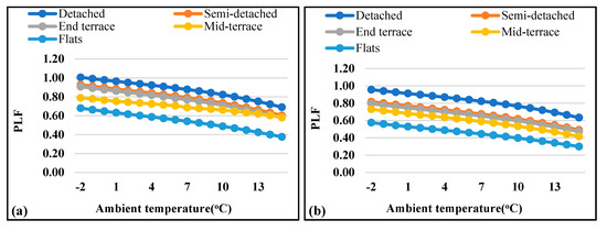
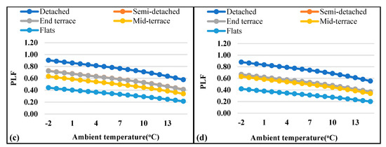
Figure 28.
Part load factor (PLF) for different property types and age periods: (a) 1900–1949, (b) 1950–1975, (c) 1976–1990, and (d) 1991–2007 onwards.
3.6.2. Energy Consumption
The annual electricity consumption depends on property type, age period, COP value, and control mode. The old age period consumes more electrical energy due to poor insulation and higher heat demands for the same property type. Among all the property type and age periods considered, the detached buildings with the age period of (1900–1949) consumed the highest energy with poor thermal inertia, while the flats with the age period (1991–2007 onwards) consumed the least energy due to lower heat demands.
3.6.3. Performance Improvement with Operating Mode of Operation (VSM vs. FSM)
The change in the mode of control and heat supply temperature impacts the system COPs and energy consumption of all property types and age periods, but with different percentage amounts. The COP values during FSM were smaller than VSM with the comparative results and improvement displayed in Figure 29, and the energy savings displayed in Figure 30. For all age periods, the highest percentage (%) improvement in COP was possible for the flats (C1), and the reason for this is the higher cycling losses and lower part load factor values for each building type and all age periods during FSM, followed by C2 and C3.
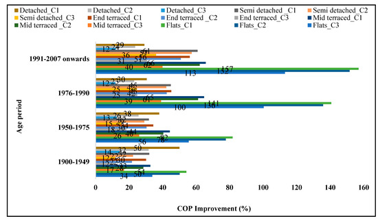
Figure 29.
HP annual COP improvement (%) due to operating mode of control (VSM vs. FSM).
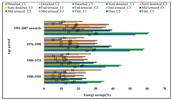
Figure 30.
HP annual energy savings (%) due to operating mode of control (VSM vs. FSM).
The lowest improvement (%) in COP occurred in the detached type (C3) for all age periods except for the first age period (1900–1949), where the lowest improvement occurred for the end-terraced (C3) buildings with a value of 11.67%. The minimum COP improvement occurred in the case of the detached buildings with only a 10–12% (C3) improvement possible for the detached building. The lowest improvement for VSM vs. FSM is because of reduced cycling losses.
4. Conclusions
The ASHP annual COP in Belfast climatic conditions was assessed for five different property types based on the developed protype testing and modelling results in two control modes and at three heat supply temperatures. The heat supply temperature and control mode of operation have a significant impact on the system performance, but improve at different percentage (%) efficiencies according to the property type and age period. The VSM operation has drawbacks with the compressor efficiencies, and this has been experimentally established, but the annual COP values were improved. The following major conclusions could be extracted from the study.
- (a)
- The annual performance is improved with the VSM of control in comparison to the FSM of control, but at the cost of higher initial cost associated with control devices. The payback period for additional control devices was 2.8 years at the lower heat supply temperature of 35 °C (C1), and increase to 3.7 years at the higher heat supply temperature of 55 °C (C3). The VSM of control for capacity adjustment is more beneficial in terms of the annual COP due to the match between the load demand and heat supplied compared to the FSM. This was also reported in the literature [55,56].
- (b)
- Among the considered cases (C1, C2, C3) and all property types with different age periods, a maximum energy savings (VSM vs. FSM) of up to 61% was possible with the flats type (C1) with the age period of 1991–2007 onwards. The reason was the lower speed operation of the system below the nominal value and the increased cycling losses in FSM.
- (c)
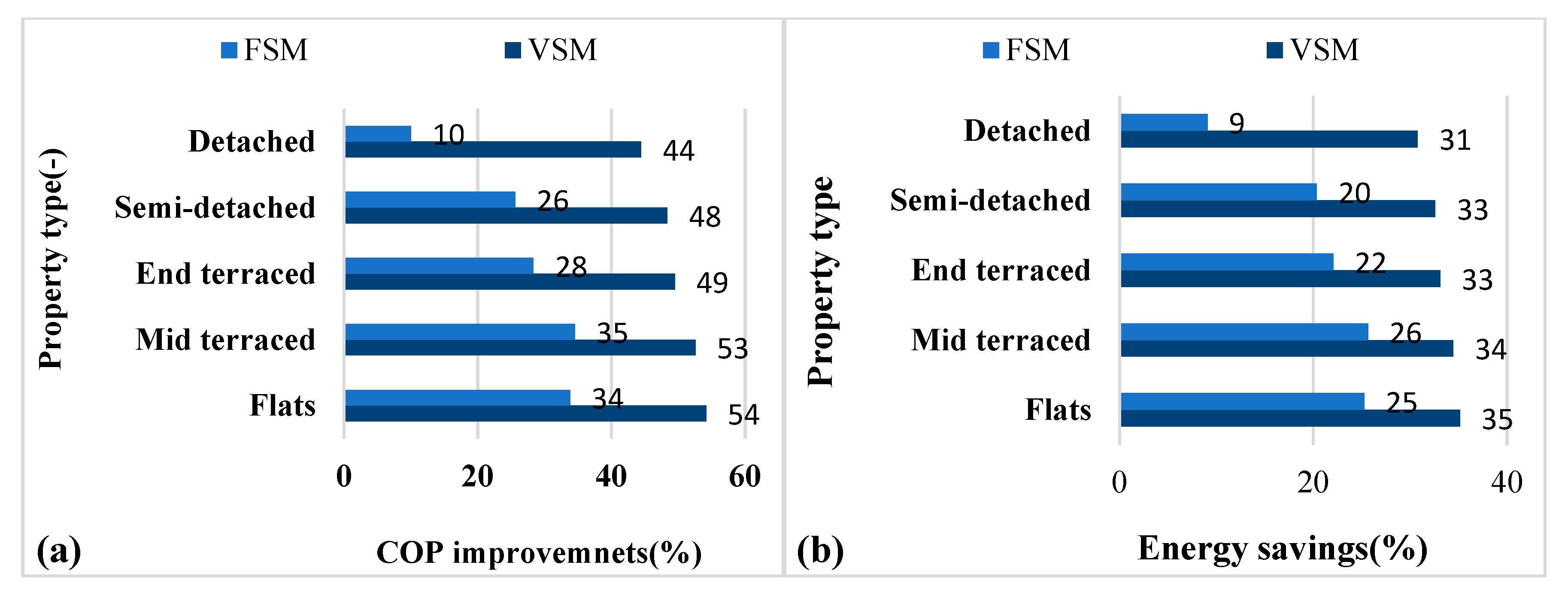
- The lower heat supply temperature has a significant impact on the annual performance improvement for all property types. The COP improvement with the HP (VSM) of up to 54% and energy savings of 35% was possible due to the control mode for the flats type (1900–1949) at the lower supply temperature. The respective improvement with the COP and energy reduced to 34% and 25%, respectively, during the FSM.
Author Contributions
Conceptualization, N.H. and M.-J.H.; methodology, M.-J.H.; software, M.A.; validation, M.A.; formal analysis, M.A.; investigation, M.A.; resources C.W. and D.C.; data curation, M.A.; writing—original draft preparation, M.A.; writing—review and editing, M.-J.H.; visualization, M.A.; supervision, N.H. and M.-J.H.; project administration, N.H. and M.-J.H.; funding acquisition, N.H. and M.-J.H. All authors have read and agreed to the published version of the manuscript.
Funding
The SPIRE 2 project is supported by the European Union’s INTERREG VA Program (Grant Number: IVA5038), managed by the Special EU Programs Body (SEUP(B). The views and opinions expressed in this paper do not necessarily reflect those of the European Commission or SEUPB.
Institutional Review Board Statement
Not applicable.
Informed Consent Statement
Not applicable.
Data Availability Statement
Not applicable.
Conflicts of Interest
The authors declare no conflict of interest.
Abbreviations
| ASHP | air source heat pump |
| COP | coefficient of performance (-) |
| CO2 | carbon dioxide (-) |
| C1 | case study 1 (35 °C fixed heat supply temperature) |
| C2 | case study 2 (45 °C fixed heat supply temperature) |
| C3 | case study 3 (55 °C fixed heat supply temperature) |
| DB | dry bulb temperature (°C) |
| SCOP | seasonal coefficient of performance (-) |
| DB | dry bulb (°C) |
| EH | electric heater requirements (KWh) |
| EIR | electric input ratio (−) |
| EWT | entering water temperature (°C) |
| FSM | fixed speed mode (-) |
| PLF | part load factor (−) |
| PLR | part load ratio (−) |
| RMSE | root-mean-square error |
| VSM | variable speed mode (-) |
| WST | water supply temperature (°C) |
| WB | wet bulb (°C) |
| RH (%) | relative humidity (-) |
| PID | proportional integral derivative |
| RPM | revolution per minute |
| HD | heat demand (kW) |
| HC | heating capacity (kW) |
| A2W35 | ambient temperature of 2 °C with water temperature of 35 °C |
| Symbols | |
| water specific heat capacity (kJ/kg·K) | |
| heating capacity (kW) | |
| refrigerant mass flow rate (kg/s) | |
| pressure ratio (-) | |
| ambient temperature (°C) | |
| water mass flow rates (kg/s) in a closed circuit | |
| difference between supplied and entering water temperature to the HP | |
| isentropic efficiency (%) | |
| volumetric efficiency (%) | |
| refrigerant specific volume at the compressor suction (m3·kg−1) | |
| swept volume (m3) | |
| enthalpy difference (kJ/kg) | |
| isentropic enthalpy (kJ/kg) | |
| total electric power consumption (kW) | |
| compressor electric power consumption (kW) | |
| auxiliaries power consumption (kW) | |
| Greek symbols | |
| relative humidity (%) | |
| density (kg/m3) | |
| frequency (Hz) |
References
- United Nations Environment Programme. Renewables 2020 Global Status Report. 2020. Available online: https://www.ren21.net/wp-content/uploads/2019/05/gsr_2020_full_report_en.pdf (accessed on 18 May 2021).
- European Parliament. EU Directive on the Energy Performance of Buildings (Recast) (2010/31/EU). 2010. Available online: https://ec.europa.eu/energy/topics/energy-efficiency/energy-efficient-buildings/energy-performance-buildings-directive_en (accessed on 18 May 2021).
- Department for Business, Energy and Industrial Strategy. Energy Consumption in the UK 2020. Available online: https://www.gov.uk/government/statistics/energy-consumption-in-the-uk (accessed on 18 May 2021).
- Department of Energy and Climate Change. Provisional Estimates of UK Greenhouse Gas Emissions for 2015, Including Quarterly Emissions for 4th Quarter 2015. Available online: https://www.gov.uk/government/statistics/provisional-uk-greenhouse-gas-emissions-national-statistics-2015 (accessed on 24 September 2020).
- Druckman, A.; Jackson, T. Household energy consumption in the UK: A highly geographically and socio-economically disaggregated model. Energy Policy 2008, 36, 3177–3192. [Google Scholar] [CrossRef] [Green Version]
- Emissions from Heat. Technical Report, Department of Energy and Climate Change. Available online: https://www.gov.uk/government/statistics/uk-emissions-from-heat (accessed on 27 July 2020).
- Net Zero by 2050: A Roadmap for the Global Energy System. Available online: https://www.iea.org/events/net-zero-by-2050-a-roadmap-for-the-global-energy-system (accessed on 5 October 2021).
- Parliament of the United Kingdom. Climate Change Act (2008). Available online: http://www.legislation.gov.uk/ukpga/2008/27/pdfs/ukpga_20080027_en.pdf (accessed on 21 May 2019).
- CCC Net Zero. The UK’s Contribution to Stopping Global Warming. 2019. Available online: https://www.theccc.org.uk/publication/net-zero-the-uks-contribution-to-stopping-global-warming/ (accessed on 18 May 2021).
- GOV.UK. Spring Statement 2019: What You Need to Know—GOV.UK 2019. Available online: https://www.gov.uk/government/news/spring-statement-2019-what-you-need-to-know (accessed on 18 May 2021).
- Carroll, P.; Chesser, M.; Lyons, P. Air Source Heat Pumps field studies: A systematic literature review. Renew. Sustain. Energy Rev. 2020, 134, 110275. [Google Scholar] [CrossRef]
- Jeter, S.M.; Wepfer, W.J.; Fadel, G.M.; Cowden, N.E.; Dymfk, A.A. Variable speed drive heat pump performance. Energy 1987, 12, 1289–1298. [Google Scholar] [CrossRef]
- Madani, H.; Claesson, J.; Lundqvist, P. Capacity control in ground source heat pump systems part II: Comparative analysis between on/off controlled and variable capacity systems. Int. J. Refrig. 2011, 34, 1934–1942. [Google Scholar] [CrossRef]
- European Standard EN 14511-3—Air Conditioners, Liquid Chilling Packages and Heat Pumps with Electrical Driven Compressors for Space Heating and Cooling-Part 3, Test Methods. 2018. Available online: https://www.iea.org/policies/7031-en-14511-22018-test-methods-and-standards-for-air-conditioners-liquid-chilling-packages-and-heat-pumps (accessed on 27 July 2020).
- Bundesamt für Wirtschaft und Ausfuhrkontrolle. Erneuerbare Energien Wärmepumpen mit Prüfnachweis; Technical Report; Bundesamt für Wirtschaft und Ausfuhrkontrolle: Eschborn, Germany, 2016.
- Qureshi, T.Q.; Tassou, S.A. Variable-speed capacity control in refrigeration systems. Appl. Therm. Eng. 1996, 16, 103–113. [Google Scholar] [CrossRef]
- Wong, A.K.H.; James, R.W. Capacity control of a refrigeration system using a variable speed compressor. Build. Serv. Eng. Res. Technol. 1988, 9, 63–68. [Google Scholar]
- Wong, A.K.H.; James, R.W. Influence of control systems on the performance of refrigeration systems. Aust. Refrig. Air Cond. Heat. 1989, 43, 21–36. [Google Scholar]
- Tassou, S.A.; Qureshi, T.Q. Performance of a variable speed inverter/motor drive for refrigeration applications. Comput. Control Eng. J. 1994, 5, 193–199. [Google Scholar] [CrossRef]
- Tassou, S.A.; Marquand, C.J.; Wilson, D.R. The effects of capacity modulation on the performance of vapour compression heat pump systems. In Proceedings of the International Conference, Forward Swept Wing Aircraft, Bristol, UK, 24–26 March 1982. [Google Scholar]
- Munari, P.; Da Riva, E.; Del Col, D.; Mantovan, M. Energy efficiency of variable capacity ground source heat pumps. In Proceedings of the AS-Alternative Sources/ISPHC11-International Sorption Heat Pump Conference, Padua, Italy, 5–7 April 2011. [Google Scholar]
- Karlsson, F.; Fahlen, P. Improving efficiency of hydronic heat pump heating systems. In Proceedings of the 21st International Congress of Refrigeration, Washington, DC, USA, 17–22 August 2003. [Google Scholar]
- Karlsson, F.; Fahlen, P. Capacity—Controlled ground source heat pumps in hydronic heating systems. Int. J. Refrig. 2007, 30, 221–229. [Google Scholar] [CrossRef]
- Adhikari, R.S.; Aste, N.; Manfren, M.; Marini, M. Energy Savings through Variable Speed Compressor Heat Pump Systems. Energy Procedia 2012, 14, 1337–1342. [Google Scholar] [CrossRef] [Green Version]
- Miller, W.A. Laboratory examination and seasonal analyses of the dynamic losses for a continuously variable-speed heat pump. NASA STI/Recon Tech. Rep. N 1988, 94, 1246–1268. Available online: https://ui.adsabs.harvard.edu/#abs/1988STIN...8911174M/abstract (accessed on 27 July 2020).
- Tassou, S.A.; Qureshi, T.Q. Comparative performance evaluation of positive displacement compressors in variable-speed refrigeration applications. Int. J. Refrig. 1998, 21, 29–41. [Google Scholar] [CrossRef]
- Halozan, H. Inverter-driven heat pumps for hydronic systems. ASHRAE Trans. 1988, 1269–1278. Available online: https://heatpumpingtechnologies.org/publications/inverter-driven-heat-pumpsanalysis-of-heat-pump-units-and-systems (accessed on 18 May 2021).
- Lande, J. Tests on Air-To-Air Heat Pumps, with and without Inverter Control; Royal Institute of Technology: Stockholm, Sweden, 1992; Volume 92, p. 36. (In Swedish) [Google Scholar]
- Tassou, S.A.; Marquand, C.J. Comparison of the performance of capacity controlled and conventional on/off controlled heat pumps. Appl. Energy 1983, 14, 241–256. [Google Scholar] [CrossRef]
- Bergman, A. Impact of on/off Control of Heat Pumps Laboratory Testing; Byggforskningsrådet R111: Stockholm, Sweden, 1985; 67p. (In Swedish) [Google Scholar]
- Karlsson, F. Capacity Control of Residential Heat Pump Heating Systems. Ph.D. Thesis, Chalmers Tekniska Högskola, Göteborg, Sweden, 2007. [Google Scholar]
- Garstang, S.W. Variable frequency speed control of refrigeration compressors, Part 1. Air Cond. Heat.-Março 1990, 44, 21–23. [Google Scholar]
- Zhao, L.; Zhao, L.L.; Zhang, Q.; Ding, G.L. Theoretical and basic experimental analysis on load adjustment of geothermal heat pump systems. Energy Convers. Manag. 2003, 44, 1–9. [Google Scholar] [CrossRef]
- Karlsson, F.; Fahlen, P. Impact of design and thermal inertia on the energy saving potential of capacity-controlled heat pump heating systems. Int. J. Refrig. 2008, 31, 1094–1103. [Google Scholar] [CrossRef]
- Aprea, C.; Mastrullo, R.; Renno, C. Experimental analysis of the scroll compressor performances varying its speed. Appl. Therm. Eng. 2006, 26, 983–992. [Google Scholar] [CrossRef]
- Aprea, C.; Mastrullo, R.; Renno, C. Determination of the compressor optimal working conditions. Appl. Therm. Eng. 2009, 29, 1991–1997. [Google Scholar] [CrossRef] [Green Version]
- Cuevas, C.; Lebrun, J. Testing and modelling of a variable speed scroll compressor. Appl. Therm. Eng. 2009, 29, 469–478. [Google Scholar] [CrossRef]
- Madani, H.; Claesson, J.; Ahmadi, N.; Lundqvist, P. Experimental Analysis of a Variable Capacity Heat Pump System Focusing on the Compressor, and Inverter Loss Behaviour. In Proceedings of the International Refrigeration and Air Conditioning Conference, West Lafayette, IN, USA, 12–15 July 2010; Available online: https://docs.lib.purdue.edu/cgi/viewcontent.cgi?article=2062&context=iracc (accessed on 27 July 2020).
- Hewitt, N.J.; Huang, M.J.; Anderson, M.; Quinn, M. Advanced air source heat pumps for UK and European domestic buildings. Appl. Therm. Eng. 2011, 31, 3713–3719. [Google Scholar] [CrossRef]
- Quinn, M. The Development of a Capacity Controlled Advanced Cycle Air Source Heat Pump for Domestic Retrofit Applications. Ph.D. Thesis, Ulster University, Coleraine, UK, 2012. Available online: https://ethos.bl.uk/OrderDetails.do?did=1&uin=uk.bl.ethos.592665 (accessed on 27 July 2020).
- Abid, M.; Hewitt, N.; Huang, M.J.; Wilson, C.; Cotter, D. Experimental Study of the Heat Pump with Variable Speed Compressor for Domestic Heat Load Applications. In Proceedings of the 25th Compressor Engineering, Refrigeration, Air-Conditioning, and High-Performance Buildings, West Lafayette, IN, USA, 24–28 May 2021; Available online: https://docs.lib.purdue.edu/cgi/viewcontent.cgi?article=3677&context=icec (accessed on 29 May 2021).
- Abid, M.; Hewitt, N.; Huang, M.J.; Wilson, C.; Cotter, D. Heat Supply Temperature Impact on the Seasonal Cost of Low Carbon Domestic Heat Pump Technology. 2020. Available online: https://www.enerarxiv.org/page/thesis.html?id=2685 (accessed on 29 May 2021).
- Oughton, D.R.; Hodkinson, S.L.; Kell’s, F. Heating and Air-Conditioning of Buildings Tenth Edition; Elsevier: Amsterdam, The Netherlands, 2008; Available online: http://docshare04.docshare.tips/files/22696/226963577.pdf (accessed on 29 May 2020).
- Carbon Trust Report, August 2020. Heat Pump Retrofit in London. Available online: https://www.carbontrust.com/resources/heat-pump-retrofit-in-london (accessed on 30 March 2021).
- Klein, S.A.; Beckman, W.A.; Mitchell, J.W.; Duffie, J.A.; Duffie, N.A.; Freeman, T.L.; Mitchell, J.C.; Braun, J.E.; Evans, B.L.; Kummer, J.P.; et al. TRNSYS 17: A Transient System Simulation Program; Solar Energy Laboratory, University of Winsconsin: Madison, WI, USA, 2010. [Google Scholar]
- ASHRAE. Guideline 2-2010, Engineering Analysis of Experimental Data; ASHRAE: Atlanta, GA, USA, 1986; Available online: https://www.techstreet.com/standards/guideline-2-2010-ra-2014-180engineering-analysis-of-experimental-data?product_id=1873287 (accessed on 29 May 2020).
- Correa, F.; Cuevas, C. Air-water heat pump modelling for residential heating and domestic hot water in Chile. Appl. Therm. Eng. 2018, 143, 594–606. [Google Scholar] [CrossRef]
- Wolfram Research, Inc. Mathematica, Version 12.2; Wolfram Research, Inc.: Champaign, IL, USA, 2020. [Google Scholar]
- Madonna, F.; Bazzocchi, F. Annual performances of reversible air-to-water heat pumps in small residential buildings. Energy Build. 2013, 65, 299–309. [Google Scholar] [CrossRef]
- Cabrol, L.; Rowley, P. Towards low carbon homes—A simulation analysis of building-integrated air-source heat pump systems. Energy Build. 2012, 48, 127–136. [Google Scholar] [CrossRef] [Green Version]
- Kinab, E.; Marchio, D.; Riviere, P.; Zoughaib, A. Reversible heat pump model for seasonal performance optimization. Energy Build. 2010, 42, 2269–2280. [Google Scholar] [CrossRef]
- Dongellini, M.; Naldi, C.; Morini, G.L. Seasonal performance evaluation of electric air-to-water heat pump systems. Appl. Therm. Eng. 2015, 90, 1072–1081. [Google Scholar] [CrossRef]
- Mader, G.; Madani, H. Capacity control in air-water heat pumps: Total cost of ownership analysis. Energy Build. 2014, 81, 296–304. [Google Scholar] [CrossRef]
- Myers, M.; Kourtza, E.; Kane, D.; Harkin, S. The Cost of Installing Heating Measures in Domestic Properties; A Delta-EE Report for the Department for Business, Energy, and Industrial Strategy BEIS; London, UK. Final Report 2018; Research Paper Number: 2020/028; Delta Energy and Environment Ltd.: Edinburgh, UK, 2020. [Google Scholar]
- Szreder, M.; Miara, M. Impact of Compressor Drive System Efficiency on Air Source Heat Pump Performance for Heating Hot Water. Sustainability 2020, 12, 521. [Google Scholar] [CrossRef]
- Abid, M.; Hewitt, N.; Huang, M.-J.; Wilson, C.; Cotter, D. Domestic Retrofit Assessment of the Heat Pump System Considering the Impact of Heat Supply Temperature and Operating Mode of Control—A Case Study. Sustainability 2021, 13, 10857. [Google Scholar] [CrossRef]


Publisher’s Note: MDPI stays neutral with regard to jurisdictional claims in published maps and institutional affiliations. |
© 2021 by the authors. Licensee MDPI, Basel, Switzerland. This article is an open access article distributed under the terms and conditions of the Creative Commons Attribution (CC BY) license (https://creativecommons.org/licenses/by/4.0/).