
Evaluation of Greenhouse Gas Emissions from Reservoirs: A Review


Abstract
:1. Introduction
2. Assessment of GHG Emissions from the Reservoirs
- CO2 emission expressed in kg CO2/MWh as a function of the area-to-electricity ratio (ATER, km2/GWh) and reservoir area (S, km2):
- CH4 emission expressed in kg CH4/MWh as a function of the reservoir age (A, years), area-to-electricity ratio (ATER, km2/GWh) and maximum temperature (Tmax, °C):
- CH4 bubbling emission:
- CH4 diffusive emission:
- CH4 storage emission:where S is the reservoir area (m2), TP is the concentration of total phosphorous (μmol/L), and DOC is the concentration of dissolved organic carbon (mg C/L).
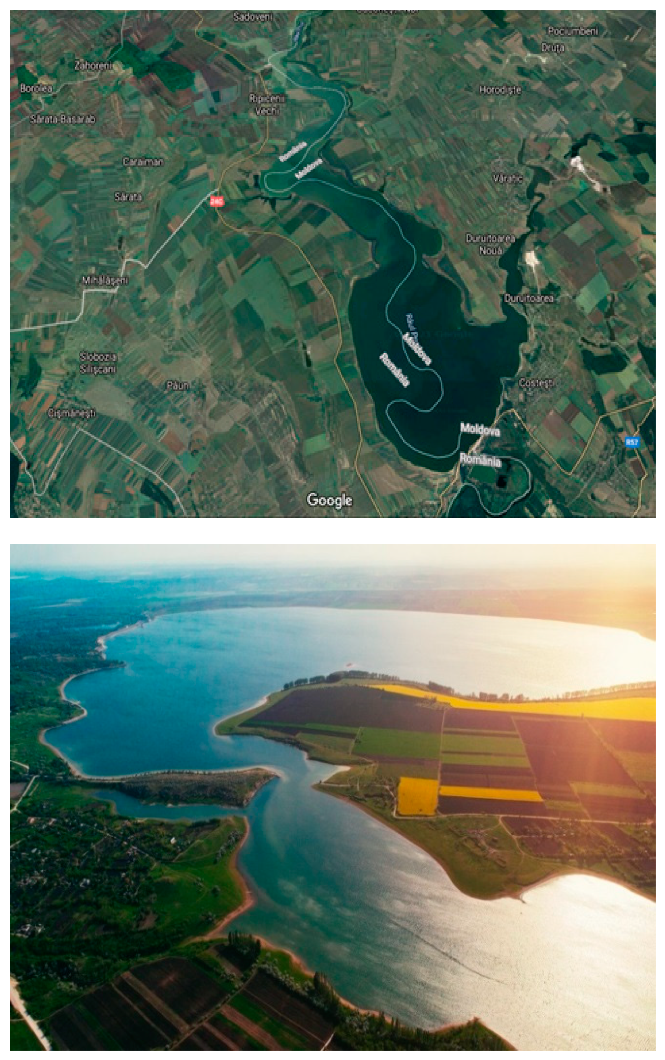
3. Case Study: The Stânca-Costești Multipurpose Reservoir
4. Results and Discussions
5. Conclusions
Author Contributions
Funding
Institutional Review Board Statement
Informed Consent Statement
Data Availability Statement
Acknowledgments
Conflicts of Interest
References
- Levasseur, A.; Mercier-Blais, S.; Prairie, Y.T.; Tremblay, A.; Turpin, C. Improving the accuracy of electricity carbon footprint: Estimation of hydroelectric reservoir greenhouse gas emissions. Renew. Sust. Energ. Rev. 2021, 136, 110433. [Google Scholar] [CrossRef]
- IPCC (Intergovernmental Panel on Climate Change). 2006 IPCC Guidelines for National Greenhouse Gas Inventories; Eggleston, H.S., Buendia, L., Miwa, K., Ngara, T., Tanabe, K., Eds.; Institute for Global Environmental Strategies (IGES): Kanagawa, Japan, 2006. [Google Scholar]
- World Bank. Greenhouse Gases from Reservoirs Caused by Biogeochemical Processes; World Bank: Washington, DC, USA, 2017; Available online: https://openknowledge.worldbank.org/handle/10986/29151 (accessed on 16 December 2020).
- Almeida, R.M.; Paranaíba, J.R.; Barbosa, Í.; Sobek, S.; Kosten, S.; Linkhorst, A.; Mendonça, R.; Quadra, G.; Roland, F.; Barros, N. Carbon dioxide emission from drawdown areas of a Brazilian reservoir is linked to surrounding land cover. Aquat. Sci. 2019, 81, 68. [Google Scholar] [CrossRef] [Green Version]
- Barros, N.; Cole, J.J.; Tranvik, L.J.; Prairie, Y.T.; Bastviken, D.; Huszar, V.L.M.; del Giorgio, P.; Roland, F. Carbon emission from hydroelectric reservoirs linked to reservoir age and latitude. Nat. Geosci. 2011, 4, 593–596. [Google Scholar] [CrossRef]
- Bastviken, D.; Cole, J.; Pace, M.; Tranvik, L. Methane emissions from lakes: Dependence of lake characteristics, two regional assessments, and a global estimate. Glob. Biogeochem. Cycles 2004, 18, GB4009. [Google Scholar] [CrossRef]
- Bastviken, D.; Tranvik, L.J.; Downing, J.A.; Crill, P.M.; Enrich-Prast, A. Freshwater methane emissions offset the continental carbon sink. Science 2011, 331, 50. [Google Scholar] [CrossRef] [Green Version]
- Chen, H.; Wu, Y.Y.; Yuan, X.Z.; Gao, Y.S.; Wu, N.; Zhu, D. Methane emissions from newly created marshes in the drawdown area of the Three Gorges Reservoir. J. Geophys. Res. 2009, 114, D18301. [Google Scholar] [CrossRef]
- Chen, Z.; Ye, X.; Huang, P. Estimating Carbon Dioxide (CO2) Emissions from Reservoirs Using Artificial Neural Networks. Water 2018, 10, 26. [Google Scholar] [CrossRef] [Green Version]
- Deemer, B.R.; Harrison, J.A.; Li, S.; Beaulieu, J.J.; Delsontro, T.; Barros, N.; Bezerra-Neto, J.F.; Powers, S.M.; Dos Santos, M.A.; Vonk, J.A. Greenhouse gas emissions from reservoir water surfaces: A new global synthesis. Bioscience 2016, 66, 949–964. [Google Scholar] [CrossRef]
- Du, H.L.; Li, Z.; Guo, J.S. Carbon footprint of a large hydropower project in the upstream of the Yangtze: Following ISO14067. Resour. Environ. Yangtze Basin 2017, 26, 1102–1110. [Google Scholar]
- Gallagher, J.; Styles, D.; McNabola, A.; Williams, A.P. Life cycle environmental balance and greenhouse gas mitigation potential of micro-hydropower energy recovery in the water industry. J. Clean Prod. 2015, 99, 152–159. [Google Scholar] [CrossRef]
- Galy-Lacaux, C.; Delmas, R.; Kouadio, J.; Richard, S.; Gosse, P. 1999, Long-term Greenhouse Gas Emissions from Hydroelectric Reservoirs in Tropical Forest Regions. Glob. Biogeochem. Cycles 1999, 13, 503–517. [Google Scholar] [CrossRef]
- Jiang, T.; Shen, Z.; Liu, Y.; Hou, Y. Carbon Footprint Assessment of Four Normal Size Hydropower Stations in China. Sustainability 2018, 10, 2018. [Google Scholar] [CrossRef] [Green Version]
- Kadiyala, A.; Kommalapati, R.; Huque, Z. Evaluation of the Life Cycle Greenhouse Gas Emissions from Hydroelectricity Generation Systems. Sustainability 2016, 8, 539. [Google Scholar] [CrossRef] [Green Version]
- Li, S.; Zhang, Q. Carbon emission from global hydroelectric reservoirs revisited. Environ. Sci. Pollut. Res. 2014, 21, 13636–13641. [Google Scholar] [CrossRef] [PubMed]
- Li, X.; Gui, F.; Li, Q. Can Hydropower Still Be Considered a Clean Energy Source? Compelling Evidence from a Middle-Sized Hydropower Station in China. Sustainability 2019, 11, 4261. [Google Scholar] [CrossRef] [Green Version]
- Mäkinen, K.; Khan, S. Policy considerations for greenhouse gas emissions from freshwater reservoirs. Water Altern. 2010, 3, 91–105. [Google Scholar]
- Mosher, J.J.; Fortner, A.M.; Phillips, J.R.; Bevelhimer, M.S.; Stewart, A.J.; Troia, M.J. Spatial and Temporal Correlates of Greenhouse Gas Diffusion from a Hydropower Reservoir in the Southern United States. Water 2015, 7, 5910–5927. [Google Scholar] [CrossRef] [Green Version]
- Prakash, R.; Bhat, I.K. Life cycle greenhouse gas emissions estimation for small hydropower schemes in India. Energy 2012, 44, 498–508. [Google Scholar]
- Prairie, Y.T.; Alm, J.; Beaulieu, J.; Barros, N.; Battin, T.; Cole, J.; del Giorgio, P.; Del Sontro, T.; Guérin, F.; Harby, A.; et al. Greenhouse gas emissions from freshwater reservoirs: What does the atmosphere see? Ecosystems 2017, 21, 1058–1071. [Google Scholar] [CrossRef]
- Prairie, Y.T.; Alm, J.; Harby, A.; Mercier-Blais, S.; Nahas, R. The GHG Reservoir Tool (Gres) Technical documentation v2.1 (2019-08-21). UNESCO/IHA research project on the GHG status of freshwater reservoirs; Joint publication of the UNESCO Chair in Global Environmental Change and the International Hydropower Association: London, UK, 2017; Available online: https://www.hydropower.org/publications/the-ghg-reservoir-tool-g-res-technical-documentation (accessed on 30 March 2021).
- Prairie, Y.T.; Mercier-Blais, S.; Harrison, J.A.; Soued, C.; Del Giorgio, P.; Harby, A.; Alm, J.; Chanudet, V.; Nahas, R. A new modelling framework to assess biogenic GHG emissions from reservoirs: The G-res, tool. Environ. Model Softw. 2021, 143, 105117. [Google Scholar] [CrossRef]
- Rosa, L.P.; dos Santos, M.A.; Matvienko, B.; Sikar, E. Hydroelectric reservoirs and global warming. In Proceedings of the RIO 02—World Climate and Energy Event, Rio de Janeiro, Brazil, 6–11 January 2002; pp. 123–129. Available online: http://www.rio12.com/rio02/proceedings/pdf/123_Rosa.pdf (accessed on 10 April 2021).
- Rosa, L.P.; dos Santos, M.A.; Matvienko, B.; dos Santos, E.O.; Sikar, E. Greenhouse Gases Emissions by Hydroelectric Reservoirs in Tropical Regions. Clim. Chang. 2004, 66, 9–21. [Google Scholar] [CrossRef]
- Scherer, L.; Pfister, S. Hydropower’s Biogenic Carbon Footprint. PLoS ONE 2016, 11, e0161947. [Google Scholar] [CrossRef] [Green Version]
- Song, C.; Gardner, K.H.; Klein, S.J.W.; Souza, S.P.; Mo, W. Cradle-to-grave greenhouse gas emissions from dams in the United States of America. Renew. Sustain. Energ. Rev. 2018, 90, 945–956. [Google Scholar] [CrossRef] [Green Version]
- St. Louis, V.L.; Kelly, C.A.; Duchemin, É.; Rudd, J.W.M.; Rosenberg, D.M. Reservoir surfaces as sources of greenhouse gases to the atmosphere: A global estimate. BioScience 2000, 50, 766–775. [Google Scholar] [CrossRef]
- Suwanit, W.; Gheewala, S.H. Life cycle assessment of mini-hydropower plants in Thailand. Int. J. LCA 2011, 16, 849–858. [Google Scholar] [CrossRef]
- Zhang, Q.F.; Karney, B.; MacLean, H.L.; Feng, J.C. Life-cycle inventory of energy use and greenhouse gas emissions for two hydropower projects in China. J. Infrastruct. Syst. 2007, 13, 271–279. [Google Scholar] [CrossRef] [Green Version]
- Zhang, S.R.; Pang, B.H.; Zhang, Z.L. Carbon footprint analysis of two different types of hydropower schemes: Comparing earth-rockfill dams and concrete gravity dams using hybrid life cycle assessment. J. Clean Prod. 2015, 103, 854–862. [Google Scholar] [CrossRef]
- Schlömer, S.; Bruckner, T.; Fulton, L.; Hertwich, E.; McKinnon, A.; Perczyk, D.; Roy, J.; Schaeffer, R.; Sims, R.; Smith, P.; et al. Annex III: Technology-specific cost and performance parameters. In Climate Change 2014: Mitigation of Climate Change. Contribution of Working Group III to the Fifth Assessment Report of the Intergovernmental Panel on Climate Change; Edenhofer, O., Pichs-Madruga, R., Sokona, Y., Minx, J.C., Farahani, E., Kadner, S., Seyboth, K., Adler, A., Baum, I., Brunner, S., et al., Eds.; Cambridge University Press: New York, NY, USA, 2014. [Google Scholar]
- Myhre, G.; Shindell, D.; Bréon, F.M.; Collins, W.; Fuglestvedt, J.; Huang, J.; Koch, D.; Lamarque, J.F.; Lee, D.; Mendoza, B.; et al. Anthropogenic and Natural Radiative Forcing. In Climate Change 2013: The Physical Science Basis. Contribution of Working Group I to the Fifth Assessment Report of the Intergovernmental Panel on Climate Change; Stocker, T.F., Qin, D., Plattner, G.-K., Tignor, M., Allen, S.K., Boschung, J., Nauels, A., Xia, Y., Bex, V., Midgley, P.M., Eds.; Cambridge University Press: Cambridge, UK; New York, NY, USA, 2013. [Google Scholar]
- Li, Z.; Du, H.L.; Xiao, Y.; Guo, J.S. Carbon footprints of two large hydro-projects in China: Life-cycle assessment according to ISO/TS 14067. Renew. Energy 2017, 114, 534–546. [Google Scholar] [CrossRef]
- IEA Hydropower. Annex XII: Guidelines for Quantitative Analysis of Net GHG Emissions from Reservoirs. 2012. Available online: https://www.ieahydro.org/publications/iea-hydro-reports (accessed on 23 November 2020).
- Lovelock, C.E.; Evans, C.; Barros, N.; Prairie, Y.; Alm, J.; Bastviken, D.; Beaulieu, J.J.; Garneau, M.; Harby, A.; Harrison, J.; et al. 2019 Refinement to the 2006 IPCC Guidelines for National Greenhouse Gas Inventories, Volume 4: Agriculture, Forestry and Other Land Use (Chapter 7: Wetlands); IPCC: Kanagawa, Japan, 2019. [Google Scholar]
- Goldenfum, J.A. (Ed.) UNESCO/IHA GHG Measurement Guidelines for Freshwater Reservoirs; International Hydropower Association (IHA): London, UK, 2010. [Google Scholar]
- Vilela, T.; Reid, J. Improving hydropower choices via an online and open access tool. PLoS ONE 2017, 12, e0179393. [Google Scholar] [CrossRef] [Green Version]
- Bergier, I.; Bambace, L.; Ramos, F.M. GHG life cycle analysis and novel opportunities arising from emerging technologies developed for tropical dams. In Proceedings of the UNESCO-IHP Workshop on the Greenhouse Gas Status of Freshwater Reservoirs, Foz do Iguaçu, Brazil, 4–5 October 2007; Available online: https://www.researchgate.net/publication/323073413_GHG_LIFE_CYCLE_ANALYSIS_AND_NOVEL_OPPORTUNITIES_ARISING_FROM_EMERGING_TECHNOLOGIES_DEVELOPED_FOR_TROPICAL_DAMS (accessed on 15 April 2021).
- Corobov, R.; Ene, A.; Trombitsky, I.; Zubcov, E. The Prut River under Climate Change and Hydropower Impact. Sustainability 2021, 13, 66. [Google Scholar] [CrossRef]
- Dumitran, G.E.; Vuta, L.I.; Popa, B.; Popa, F. Hydrological Variability Impact on Eutrophication in a Large Romanian Border Reservoir, Stânca–Costesti. Water 2020, 12, 3065. [Google Scholar] [CrossRef]
- Zomer, R.J.; Bossio, D.A.; Sommer, R.; Verchot, L.V. Global Sequestration Potential of Increased Organic Carbon in Cropland Soils. Sci. Rep. 2017, 7, 15554. [Google Scholar] [CrossRef] [PubMed] [Green Version]
- Panagos, P.; Borrelli, P.; Poesen, J.; Ballabio, C.; Lugato, E.; Meusburger, K.; Montanarella, L.; Alewell, C. The new assessment of soil loss by water erosion in Europe. Environ. Sci. Policy 2015, 54, 438–447. [Google Scholar] [CrossRef]
- Available online: https://planiada.ro/destinatii/botosani/lacul-stanca-costesti-289 (accessed on 15 January 2021).
- Available online: https://www.hidroconstructia.com/dyn/2pub/proiecte_det.php?id=114&pg=8 (accessed on 15 January 2021).
- Fekete, B.M.; Vörösmarty, C.J.; Grabs, W. Global Composite Runoff Fields Based on Observed River Discharge and Simulated Water Balances. In UNH/GRDC Composite Runoff Fields v1.0; Complex Systems Research Center, University of New Hampshire: Durham, NH, USA; Global Runoff Data Center: Koblenz, Germany, 2000; Available online: http://www.grdc.sr.unh.edu (accessed on 1 December 2020).
- International Hydropower Association (IHA). Carbon Emissions from Hydropower Reservoirs: Facts and Myths, 2021. Available online: https://www.hydropower.org/blog/carbon-emissions-from-hydropower-reservoirs-facts-and-myths (accessed on 12 April 2021).


| System Type | GHG Areal Rate, (mg/m2/d) | CO2 Equivalent Emissions, CO2eq, (g/m2/yr) | |
|---|---|---|---|
| CH4 | CO2 | ||
| All reservoirs | 160.8 | 1207.8 | 2436.38 |
| 110–128 | 1822.68 | 2695.66–2253.76 | |
| Hydroelectric reservoirs | 32.16–150 | 1412–2415 | 914.49–2742.98 |
| Lakes | 53.6 | 790.56 | 953.73 |
| Ponds | 36.18 | 1544.52 | 1012.74 |
| Rivers | 8–131 | 29,111.64 | 10,725.03–12,251.46 |
| Wetlands | 20–84 | - | 248.20–1042.44 |
| Climate Zone | Carbon Emission, (mg/m2/d) | |
|---|---|---|
| CO2 | CH4 | |
| Reservoir surface | ||
| Boreal | 753 | 9.1 |
| Temperate | 1500 [16] | 20 [16] |
| 386 [28] | 2.8 [28] | |
| Tropical | 3097 | 91.3 |
| Drawdown area | ||
| Temperate | 2110 | 110 |
| Tropical | 3500 [16] | 300 [16] |
| 13,000 [28] | 235 [28] | |
| Climate | Diffusive Emission (Ice-Free Period) E(CO2)diff (kg CO2/ha/d) Range and Median Values |
|---|---|
| Boreal wet | (0.8–34.5) 11.8 |
| Cold temperate, moist | (4.5–86.3) 15.2 |
| Warm temperate, moist | (−10.3–57.5) 8.1 |
| Warm temperate, dry | (−12.0–31.0) 5.2 |
| Tropical, wet | (11.5–90.9) 44.9 |
| Tropical, dry | (11.7–58.7) 39.1 |
| Climate Zone | Average Values (kg CH4/ha/yr) |
|---|---|
| Cool temperate | 54.00 |
| Warm temperate/dry | 150.90 |
| Warm temperate/moist | 80.30 |
| TI | Chl-a (μg/L) | TP (μg/L) | TN (μg/L) | SD (m) | Trophic Class | Trophic State Adjustment Factor, α Range and Recommended Values |
|---|---|---|---|---|---|---|
| <30–40 | 0–2.6 | 0–12 | -<350 | >4 | Oligotrophic | 0.7 (0.7) |
| 40–50 | 2.6–20 | 12–24 | −350–650 | 2–4 | Mesotrophic | 0.7–5.3 (3) |
| 50–70 | 20–56 | 24–96 | 650–1200 | 0.5–2 | Eutrophic | 5.3–14.5 (10) |
| 70–100+ | 56->155 | 96->384 | >1200 | <0.5 | Hypereutrophic | 14.5–39.4 (25) |
| Catchment Information | Value | |
|---|---|---|
| Catchment area | 12,000 km2 | |
| Population in the catchment | 150,000 | |
| Precipitation | 380 mm/yr | |
| Catchment annual runoff | 10 m3/s [46] | |
| Community wastewater treatment | None | |
| Industrial wastewater treatment | None | |
| Land cover in the catchment area | Post-impoundment | Pre-impoundment |
| Croplands | 64% | 64% |
| Grassland | 18% | 19% |
| Forest | 16% | 16% |
| Water bodies | 2% | 1% |
| Reservoir Information | ||
| Country | Romania | |
| Longitude of dam | 27°14′00″ E | |
| Latitude of dam | 47°51′30″ N | |
| Climate zone | Temperate | |
| Water uses | flood control, water supply (10 m3/s), irrigation (0.8 km3/yr), hydroenergy, aquaculture (2.9 m3/s) | |
| Impoundment year | 1978 | |
| Power generation | 30 MW | |
| Power connection | 110 V | |
| Yearly electricity generation | 130 GWh | |
| Reservoir area | 59 km2 | |
| Reservoir volume (multiannual average) | 1.4 km3 | |
| Water Level (m above sea level) | 126 m | |
| Maximum depth | 32 m | |
| Mean depth | 23.33 m (Calculated by the G-res Tool) | |
| Littoral area | 3.59% (Calculated by the G-res Tool) | |
| Water intake depth | 28 m | |
| Soil carbon content under impounded area | 0.8 kg C/m2 | |
| Annual wind speed at 10 m | 6.6 m/s | |
| Water residence time | 11.68 yr (Calculated by the G-res Tool) | |
| Annual discharge from the reservoir | 3.8 m3/s (Calculated by the G-res Tool) | |
| River Length before Impoundment (m) | 70,000 m | |
| Reservoir mean global horizontal radiance | 3.24 kWh/m2/d | |
| Mean annual air temperature | 13.3 °C | |
| Construction information | ||
| Material excavated and/or used for construction | 500,000 m3 | |
| All concrete brought to site for the dam, tunnels, foundations | 4,000,000 m3 | |
| All steel brought to site for reinforcement, pipelines, mechanical and electrical equipment | 5000 tonne | |
| Model | Emissions | |||||||||
|---|---|---|---|---|---|---|---|---|---|---|
| CO2 | CH4 | CO2eq (GWP100 for CH4 = 34) | ||||||||
| mg/m2/d | kg/MWh | tonne/yr | mg/m2/d | kg/MWh | tonne/yr | mg/m2/d | kg/MWh | tonne/yr | ||
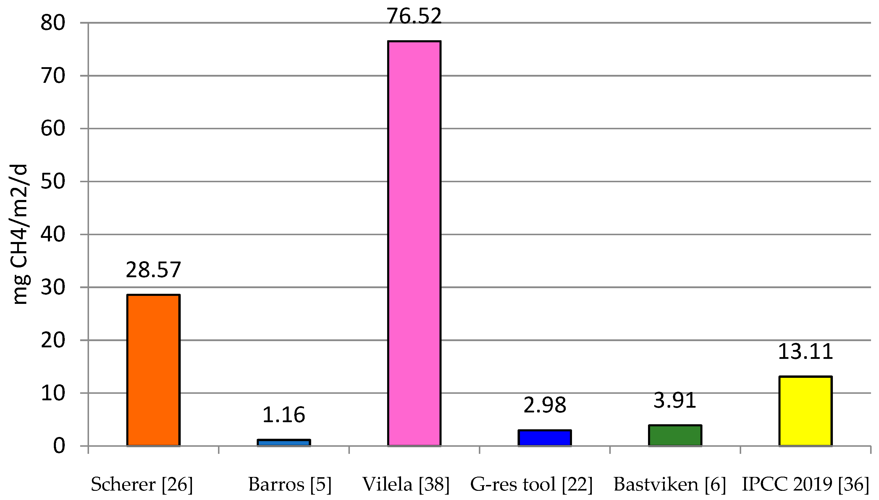
| Scherer 2016 [26] | 327.56 | 155.88 | - | 28.57 | 5.93 | - | 1298.94 | 210.72 | 27,972.67 | |
| Barros 2011 [5] | 414.35 | - | - | 1.15 | - | - | 453.65 | 73.59 | 9769.44 | |
| IPCC 2006 [2] | 520 | - | 10,124.4 | - | - | - | 520 | 77.88 | 10,124.4 | |
| IPCC 2019 [36] | - | - | - | 13.11 | - | 287.10 | 445.73 | 72.31 | 9761.40 | |
| Total | 520 | - | 10,124.4 | 13.11 | - | 287.10 | 965.73 | 150.19 | 19,885.80 | |
| Bastviken 2004 [6] | Bubbling | - | - | - | 2.46 | - | 53.88 | 83.65 | 13.57 | 1831.91 |
| Diffusion | - | - | - | 1.27 | - | 27.82 | 43.19 | 7.01 | 945.86 | |
| Storage | - | - | - | 0.18 | - | 3.93 | 6.10 | 0.99 | 133.51 | |
| Total | - | - | - | 3.91 | - | 85.63 | 132.93 | 21.56 | 2911.27 | |
| Vilela 2017 [38] | - | - | 1141.04 | 19.27 | - | 422.03 | 3497.3 | 567.34 | 15,490.06 | |
| Bergier 2007 [39] | OMCM | - | - | - | 39.24 | - | 859.321 | 1334.11 | 216.42 | 29,216.91 |
| DEM | - | - | - | 18.25 | - | 399.72 | 620.57 | 100.67 | 13,590.48 | |
| G-res tool [22] | Post-impoundment | 205.48 | - | 4425.00 | 2.98 | - | 64.21 | 306.85 | 50.83 | 6608.00 |
| Pre-impoundment | 216.44 | - | 4661.00 | 3.06 | - | 65.94 | 320.55 | 53.10 | 6903.00 | |
| Unrelated Anthropogenic Source (UAS) | 0.00 | - | 0.00 | 2.98 | - | 64.21 | 101.37 | 16.79 | 2183.00 | |
| Net reservoir emission | −10.96 | 0.00 | −236.00 | −3.06 | 0.00 | −65.94 | −115.07 | −19.06 | −2478.00 | |
| Technology | Lifecycle GHG Emission Intensity kg CO2eq/MWh |
|---|---|
| Thermal–coal | 820 |
| Thermal–natural gas | 490 |
| Biomass | 230 |
| Solar–PV | 48 |
| Hydropower | 23 |
| Nuclear | 12 |
| Wind | 12 |
Publisher’s Note: MDPI stays neutral with regard to jurisdictional claims in published maps and institutional affiliations. |
© 2021 by the authors. Licensee MDPI, Basel, Switzerland. This article is an open access article distributed under the terms and conditions of the Creative Commons Attribution (CC BY) license (https://creativecommons.org/licenses/by/4.0/).
Share and Cite
Ion, I.V.; Ene, A. Evaluation of Greenhouse Gas Emissions from Reservoirs: A Review. Sustainability 2021, 13, 11621. https://doi.org/10.3390/su132111621
Ion IV, Ene A. Evaluation of Greenhouse Gas Emissions from Reservoirs: A Review. Sustainability. 2021; 13(21):11621. https://doi.org/10.3390/su132111621
Chicago/Turabian StyleIon, Ion V., and Antoaneta Ene. 2021. "Evaluation of Greenhouse Gas Emissions from Reservoirs: A Review" Sustainability 13, no. 21: 11621. https://doi.org/10.3390/su132111621
APA StyleIon, I. V., & Ene, A. (2021). Evaluation of Greenhouse Gas Emissions from Reservoirs: A Review. Sustainability, 13(21), 11621. https://doi.org/10.3390/su132111621