Reverse Logistics Network Design and Simulation for Automatic Teller Machines Based on Carbon Emission and Economic Benefits: A Study of the Anhui Province ATMs Industry

Abstract

In recent years, mobile payments have gradually replaced cash payments, resulting in a gradual decline in the number of automatic teller machines (ATMs) demanded by banks. Through investigation and analysis, we determine four means to deal with decommissioned ATMs, and construct thereafter an ATM reverse logistics (RL_ATMs) network model, which includes suppliers, producers, warehouses, operators, maintenance centers, collection and inspection centers, disposal centers, remanufacturing centers, and recycling centers. This model is further expressed as a mixed integer linear programming (MILP) model. Given that an ATM recycling network has planned and batched characteristics, a percentage diversion method is proposed to transform a real multi-cycle problem to a single-cycle problem. The RL_ATMs network constructed in this study presents the two forms of ATMs, functional modules and the entire machine. We used the actual situations of the related companies and enterprises in Anhui Province and its surrounding areas, as well as major banks’ ATMs, as bases in using the LINGO software to solve the proposed MILP model with the objective function of minimizing costs and environmental emissions, and obtain the relevant companies’ launch operations. Lastly, we analyzed the relationship between coefficients in the percentage diversion method and calculation results, cost, and carbon emissions. Accordingly, we find that the number of remanufacturing and maintenance centers has no evident impact on the objective function, transportation costs account for a large proportion of the total cost, and emissions tax is small.

1. Introduction

Means of payment are undergoing tremendous changes from the previous cash payment to the current non-cash mobile payment [1]. Mobile payments are building a cashless world [2]. Inevitably, numerous bank automatic teller machines (ATMs) are idle [2,3], occupying bank assets and consuming bank maintenance funds. According to China entrepreneur Investment Club (CEIC) data, the global ATM ownership in 2013 was 2,785,200, which increased to 3,770,500 in 2018, and decreased to 3,451,900 in 2020 (see Figure 1). Due to the economic development, the cash deposit and withdrawal fees of various countries are different, some countries need to import or add ATMs to meet the cash demand of residents in daily life. However, in recent years, the number of ATMs has shown a downward trend, such as India and China. In China, by the end of 2020, the number of online ATMs was 1.0139 million, down 83,800 from 2019 and down 7.63% from 2019. In addition, the rise of digital cash, mobile payments and internet finance has shown an irreversible trend, marginalizing the cash transactions of banking financial institutions. It is expected that this downward trend will become more pronounced in the coming years. Decommissioning, upgrading and exporting are a good way out for ATMs. Different from automobiles, electrical appliances, etc., ATMs belong to the real estate of banks or other financial institutions and contain sensitive financial and personal information. In this case, it is a challenging topic to study the design method of an ATM reverse logistics network model with high efficiency, security, low-cost and low-emissions.

Reverse logistics is considered as one of the most effective solutions for value recovery from end-of-life and end-of-use products [4]. Reverse logistics (RLs) refers to the physical flow of items that have lost their original use value in economic activities to manufacturers or special treatment sites. It is complicated because it includes the collection, classification, processing, packaging, handling, and storage, etc., of articles.

This study designs a RL model for the recycling of used ATMs (RL_ATMs), and conducts a case study using the model for the following reasons. First, the field of RL has attracted the attention of numerous scholars [4,5,6,7] and has achieved beneficial research results. Second, used ATMs can be upgraded and modified, such as adding facial [8], finger vein [9], iris and other biometric recognition functions to ATMs, or remanufacturing their internal function modules for recycling. At present, taking most cities in China as an example, banks directly return idle or outdated ATMs to manufacturers for harmless treatment, or use commercial bidding to deal with them through a third party. Undoubtedly, this approach has adverse factors of information security and resource waste. Third, another important factor is that the strategy of recycling ATMs and steadily reducing their total number will increase economic benefits and reduce environmental pollution. In addition, solid waste recycling and supply chain emissions are increasingly being valued globally [10,11].

RL_ATMs recycling and reuse have several unique features: (1) Maintenance and upgrade are often carried out at the operators (i.e., banks) because of the immovability of the machines. Therefore, the constructed RL_ATMs model must include a closed loop composed of banks and maintenance upgrade centers. (2) The two forms of ATMs in the RL_ATMs model (i.e., functional module and the entire machine) should be discussed separately. The reason is that ATMs are a highly modular structure, which includes a card reader, host, and cash box, among others. For example, ATMs in recycling and remanufacturing centers should focus on functional modules, and in collection and inspection centers should focus on the complete machine. (3) When the RL_ATMs model is planned, its total number is required to be gradually reduced and eventually within a reasonable range; thereby, requiring the model to consider multi-period planning. (4) Security/new security features/privacy are some of the most important reasons for decommissioning ATMs long before their useful life. However, the existing research results have presented difficulty in finding a situation that meets the aforementioned four characteristics. In this case, a novel set of RL models for ATMs is constructed, and a mixed integer linear programming (MILP) model with the lowest carbon emission and the minimum cost is proposed to optimize the RL_ATMs model. Moreover, because an ATM recycling network has planned and batched characteristics, a fixed percentage diversion method to solve this dilemma is proposed, which can simplify the mathematical model of multi-period RL into a single-period problem. In this manner, the number of calculation variables and the scale of the mathematical model are reduced and the computers’ solution speed is improved. In summary, the main content of this article is to establish the RL_ATMs model, and the combination of fixed percentage diversion and the LINGO 12.0 software was used to plan and solve the model. The goal of logistics planning is to calculate the operation (whether to put into operation) and flow of each logistics node under the objective function of minimum cost and carbon emission.

The remainder of this paper is organized as follows. Section 2 provides a comprehensive literature review and summarizes the research gaps. Section 3 describes the definition of the research problem and presents the RL_ATMs model. Section 4 constructs a mathematical model and provides a solution method. Section 5 uses the proposed model and method to deal with the RL_ATMs problem according to the actual situation in Anhui Province, China, and discusses the definition of the parameters and solution results. Lastly, Section 6 concludes this research.

2. Literature Review

RL has been frequently studied owing to its outstanding economic and environmental advantages, particularly because its main areas of research (i.e., distribution planning, inventory control, and production planning) was proposed by Fleischmann [12] in 1997. In the past decades, great results have been achieved in the research of RL, such as in terms of reverse logistics network design and simulation research. In addition, some of the related studies have a “planning” subject [13]. The current study’s literature review focuses on summarizing the model framework and simulation research of RL, and eventually combining the specificity of ATMs to describe the research gap.

2.1. Reverse Logistics Network Design

There is a lot of research related to reverse logistics network design (RLND). RLND was studied for a long period to facilitate waste recycling and adapted for various scenarios (e.g., multi-echelon, multi-period, multi-product, multi-objective and stochastic). Tsai-Yun Liao [14] developed a generic mixed integer nonlinear programming model for reverse logistics network design. This is a multi-echelon reverse logistics model. It maximizes total profit by handling products returned for repair, remanufacturing, recycling, reuse, or incineration/landfill. Hao Yu and Wei Deng Solvang [4] presented a stochastic mixed integer programming model for designing and planning a generic multi-source, multi-echelon, capacitated, and sustainable reverse logistics network for WEEE management under uncertainty. Xuehong Gao [15] designed a novel stochastic reverse logistics network by reconstructing the facilities based on the existing forward logistics network. Kannan et al. [16] built an RL network design model based on carbon footprint, which can be applied to real-time case studies, such as the tire, battery, and bottling industries. Ehsan Pour Javad et al. [17] presented a multi-period closed-loop supply chain network design (in the forward and reverse chains) for a glass manufacturing industry located in the center part of Iran.

Concerning the objectives of RLND, most attention has focused on economic objectives. For instance, Md Tasbirul Islam, et al. [18] proposed a mixed-integer programming-based RL model for New South Wales, Australia that minimizes the overall cost by identifying optimal locations and sizing. Reynaldo Cruz-Rivera [5] presented a brief description of the current Mexican ELV management system and the future trends in ELV generation in Mexico. Regions with high ELV generation are identified as well as relevant factors affecting total costs in the reverse supply chain. Part of the literature used multi-objective models and adopted environmental objectives apart from economic objectives in the multi-objective modelling [19,20,21].

Concerning the model solving method of RLND, most attention has focused on the method of using software, such as CPLEX [22,23], LINGO [7,16], etc. Other methods, such as an artificial bee colony [24], variable neighborhood descent heuristics [25], NSGA-II [26], and tabu search-based methodology [27], are also used to study RL model solving. By analyzing the current situation of used ATM recycling, the current study constructed a reverse logistics model (i.e., MILP model) with the minimum cost and minimum carbon emissions as the objective function for this problem and eventually solved it using LINGO.

2.2. Simulation Research for RL

Some studies have used real case data to investigate and simulate reverse logistics scenarios in different industries, with the purpose of discussing its main challenges in economics and the environment, among others. Kinobe et al. [28] summarized the RL of the Kampala City landfill site, and meticulously analyzed the collection, reprocessing, and redistribution of reusable products in the RL network. A total of 14% of reusable products proceed to the RL network, 63% are discarded and 23% are buried. De Oliveira et al. [29] investigated the expanded polystyrene supply chain in Brazil with the aim of discussing its main challenges to the circular economy. Evidently, the main barriers are high transportation costs and numerous residents (i.e., 81% of Brazilians) lacking awareness of recycling. Kusakci et al. [30] developed an end-of-life vehicles (ELVs) RL network model that conforms to the existing directives in Turkey. This model has seven main clusters in the Istanbul Metropolitan area. The research results indicated that the current network is not profitable at a given level of ELVs, although there is room for improvement. Wang et al. [31] used the 2017 data from seven member companies of the Shanghai End-of-life Vehicle Professional Committee in China to study the efficiency of RL in the Shanghai ELVs industry. They were convinced that the company’s fixed asset investment is the key to improving its technical efficiency. De Campos, E. A. R. et al. [32] conducted surveys and interviews with 320 Brazilian supply chain executives, and performed an analysis using structural equation modeling. The results indicated that organizations that develop RL capabilities are likely to improve their economic and environmental performances. In Sweden, estimates of the number of lithium-ion batteries reaching their EOL in 2025 and the amount being recycled indicated large deviations. Tadaros et al. [33] provided decision support tools to analyze input, and optimize a future supply chain for discarded lithium–ion batteries. The main methods to obtain the data of the appeal case are as follows: (1) surveys and visits [32], (2) proportional coefficient or use of proportional coefficient to express the research results [29], (3) extension of the entire industry through partial accurate data [31], and (4) prediction of future situations [33].

The current study uses the per capita GDP data in the Anhui Statistical Yearbook to calculate the number of ATMs, and consider the operation of 48 related enterprises and companies. We conclude that the transportation cost accounts for a large proportion of the total cost. The number of some technology-based enterprises in the model has minimal effects on the total cost. We are optimistic that our research can be used as a reference after the project enters the implementation stage.

2.3. RL for ATM with a “Planning” Subject

Research on RL is spread across all walks of life, such as electronics and electrical appliances [33], construction waste recycling [34], food [35], clothing [36], product packaging [11], automobiles [37], etc. However, RL_ ATMs is considerably distinctive. First, there is no current physical project with a certain scale. Second, under the premise that mobile payment occupies the main payment method for residents, reducing the number of ATM market holdings is an urgent problem that China needs to solve. Third, the ATM structure is highly modular, and the recycling value of a single module is substantial. Lastly, RL_ATMs has a “planning” subject, and it is a planned and batch process from the ATM layout to decommissioning. At present, no research on RL_ATMs has been conducted. The research gaps are summarized as follows:

• In the constructed RL_ATMs model, ATMs have two forms (i.e., complete machine and module). Operators and maintenance centers form a closed-loop mode;
• An RL optimization model that reduces the number of ATMs remaining at the end of the RL planning cycle is proposed;
• A percentage diversion method is proposed, transforming a multi-period problem into a single-period problem, thereby simplifying the optimization of the model;
• On the basis of the actual situation in Anhui Province, China, a simulation study of RL_ATMs was conducted to provide a reference for solving the problem of oversupply of ATMs in the future.

3. Problem Definition and Modeling

3.1. Problem Description

After studying the technical manuals of ATMs and the actual dismantling analysis, these machines have been found to be a highly modular structure [38], which consists of a host, power supply, card reader (bank card throughput), movement (banknote throughput, banknote verification), administrator operation panel (located at the back of ATMs), user operation panel (located at the front of ATMs), log printer, receipt printer, cash box (storage of banknotes, recovery of counterfeit money), and box components (see Figure 2). The majority of these modules have high recycling value, such as the CPU, motherboard, and memory sticks inside the host, which can be applied continuously. Through research on the present situation of used ATMs, the main recycling processing paths are as follows:

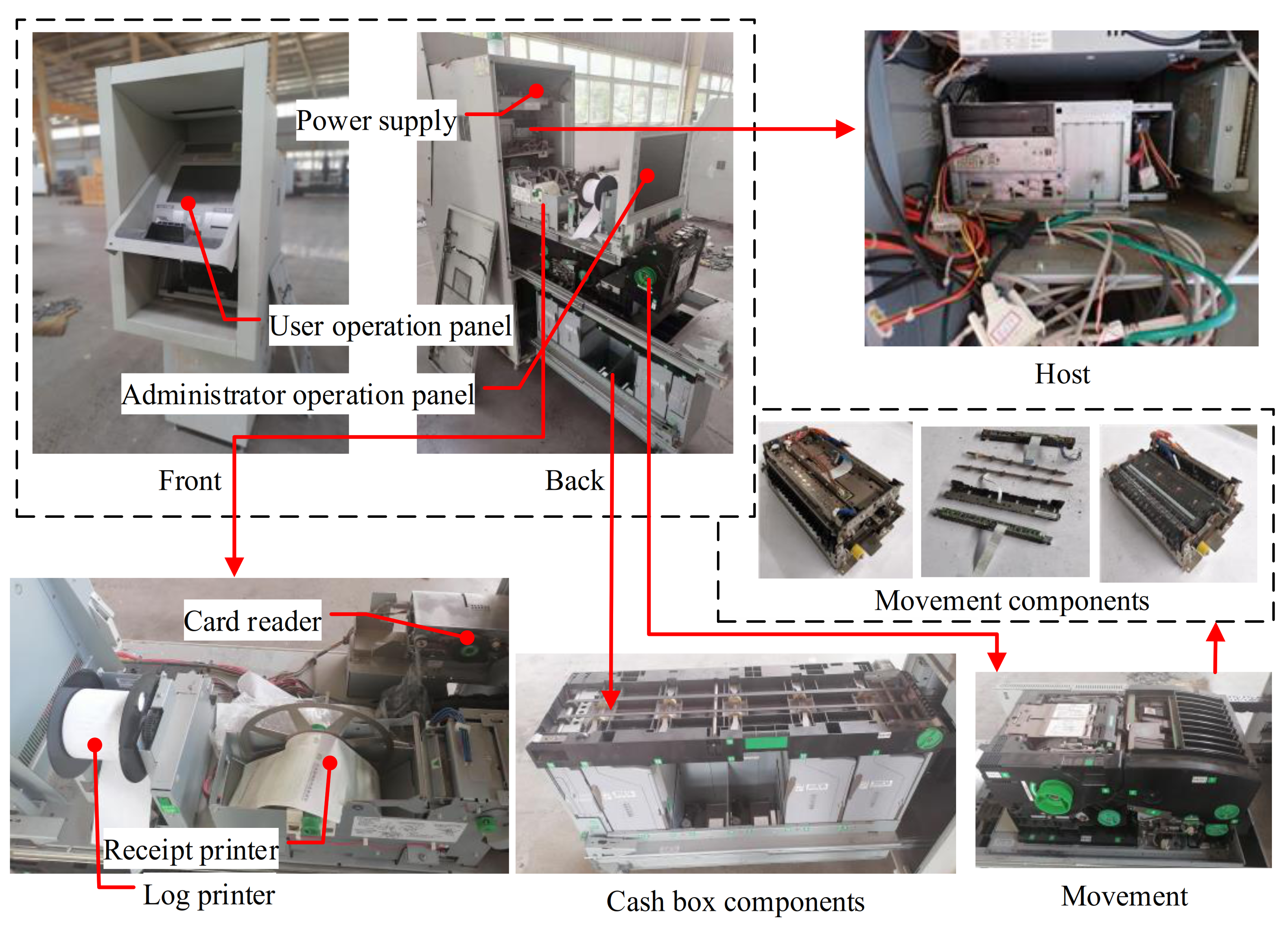
• ATMs are upgraded, such as adding facial, finger vein, iris, and other biometric recognition functions;
• The internal function modules of ATMs are remanufactured to make them recyclable and reusable;
• The internal function modules of ATMs are decomposed and disassembled components are reused in the form of parts or raw materials;
• The internal function modules of ATMs are decomposed and disassembled materials are treated as waste.

Due to the preceding content as background, an RL_ATMs model is proposed, as shown in Figure 3. This model contains four flow directions in the positive direction (solid line in the figure): S to P, P to W, W to O, M to O, and 10 flow directions in the reverse direction (dotted line in the figure): O to M, O to C, C to D, C to R, C to L, R to P, R to M, L to M, L to D, and L to S. The research focus of this article is these ten-reverse logistics.

Figure 2. ATM structure.

Figure 2. ATM structure.

Figure 3 shows that suppliers provide raw materials to producers, products manufactured by manufacturers are distributed to operators through warehouses, and maintenance centers provide necessary maintenance components to maintain and upgrade ATMs, which are forward logistics. The remainder are reverse logistics: (1) Collection and inspection centers decompose ATMs into modules, which are detected and classified by an expert group, and send the modules that meet remanufacturing conditions to remanufacturing centers; which directly disposes the modules with no recycling value in the disposal centers and send the remainder to module disassembly centers. (2) Remanufacturing centers perform remanufacturing and send the remanufactured products to maintenance centers or the producers. (3) Module disassembly and recycling centers disassemble the modules and send valuable parts to maintenance centers or suppliers; unusable parts are dealt with within disposal centers. (4) Lastly, maintenance centers directly recover the available parts or modules replaced from active ATMs.

Figure 3. A conceptual framework for the RL_ATMs.

Figure 3. A conceptual framework for the RL_ATMs.

Networks are established according to the actual ATM recycling process. Known variables in networks include the total number of ATMs in banks and estimated demand for ATMs at the end of the plan, geographic location of qualified logistics centers, and percentage of ATM diversion between logistics centers. The goal of logistics planning is to calculate the operation (whether to put into operation) and flow of each logistics node under the optimal objective function. The reverse logistics model of the majority of immovable public facilities can be solved through this network. The following assumptions and limitations are provided during the network simulation solution:

• The location and number of operators (bank branches) are known and determined;
• In the transportation cost and carbon emission calculations, the module can be regarded as the equivalent of the entire machine and converted by the coefficient K;
• The opening cost (generally including production equipment cost, worker training cost and site construction cost) of the maintenance center includes the transportation cost between itself and other operators;
• Used products are collected by collection and inspection centers, and there is no outflow;
• The total number of ATMs at the beginning of the model calculation is known, demand for ATMs at the end of solving the model is known, and the number of newly invested in ATMs is not counted during this period;
• Remanufactured, repaired, and reused modules and components can meet the needs of producers and operators.

3.2. Notation

Set and its index:

S: set of suppliers, s∈S;

P: set of producers, p∈P;

W: set of warehouses, w∈W;

O: set of operators (, o∈O;

M: set of maintenance centers, m∈M;

C: set of collection and inspection centers, c∈C;

D: set of disposal centers, d∈D;

R: set of remanufacturing centers, r∈R;

L: set of module disassembly and recycling centers, l∈L;

Boolean variables (Decision variables):

Ys,Yp,Yw,Yo,Ym,Yc,Yd,Yr,Yl:

Boolean decision variables associated with suppliers (S), producers (P), etc., module disassembly and recycling centers (L) that can have the state values open (1) or not (0);

Parameters:

DIsp, DIpw, DIwo, DIoc, DImc, DIcr, DIcl, DIcd, DIrp, DIrm, DIlm, DIls, DIld:

Distance from suppliers (S) to producers (P), from producers (P) to warehouses (W), etc., from module disassembly and recycling centers (L) to disposal centers (D) (unit: km);

PEco, PEmo:

Collection and inspection centers (C) and maintenance centers (M) account for the percentage of operators ((O) in logistics quantity;

PEdc, PErc, PElc:

Disposal centers (D), remanufacturing centers (R) and module disassembly and recycling centers (L) account for the percentage of collection and inspection centers (C) in logistics quantity;

PEpr, PEmr:

Producers (P) and maintenance centers (M) account for the percentage of remanufacturing centers (R) in logistics quantity;

PEsl, PEml, PEdl:

Suppliers (S), maintenance centers (M) and disposal centers (D) account for the percentage of module disassembly and recycling centers (L);

OCs, OCp, OCw, OCm, OCc, OCd, OCr, OCl:

Opening cost of suppliers (S), producers (P), etc., module disassembly and recycling centers (L) (unit: RMB);

PCp: cost of producers (P) using the remanufacturing module of the remanufacturing centers (R) to produce one ATM (unit: RMB);

PCm: cost of maintaining an ATM (unit: RMB);

PCc: cost of processing an ATM in the collection and inspection centers (C) (unit: RMB);

PCd: cost of disposal an ATM module (unit: RMB);

PCr: cost of remanufacturing an ATM module (unit: RMB);

PCl: cost of processing an ATM in the module disassembly and recycling centers (L) (unit: RMB);

Npw, Noc, Ncd, Ncr, Ncl, Nrp, Nrm, Nld, Nlm, Nls:

Logistics quantity from P to W, O to C, C to D, C to R, C to L, R to P, R to M, L to D, L to M and L to S;

Ns, Np, Nw, Nm, Nc, Nd, Nr, Nl:

Total processing volume of logistics centers S, P, W, M, C, D, R and L;

TN: total number of products before model calculation;

EN: estimated total number of remaining ATMs after calculating the model;

MASs, MISs: upper and lower limits of S capacity;

MAPp, MIPp: upper and lower limits of P capacity;

MAWw, MIWw: upper and lower limits of W capacity;

MAOo, MIOo: upper and lower limits of O capacity;

MAMm, MIMm: upper and lower limits of M capacity;

MACc, MICc: upper and lower limits of C capacity;

MADd, MIDd: upper and lower limits of D capacity;

MARr, MIRr: upper and lower limits of R capacity;

MALl, MILl: upper and lower limits of L capacity;

MAMm, MIMm: upper and lower limits of M capacity;

T1    transportation cost of a unit product (unit: RMB/km*piece);

T2    transportation cost of a module (unit: RMB/km*piece);

α1    remanufacturing centers (R) conversion rate;

α2    module disassembly and recycling centers (L) conversion rate;

CAi  carbon emission indicators for i, i∈(D,S, M, R, L, P) (unit: g/piece);

CT₁  carbon emission indicators during ATMs transportation (unit: g/km*piece);

CT₂  carbon emission indicators during modules transportation (unit: g/km*piece);

CF    cost function (unit: RMB);

EF    environmental emission function (unit: g);

Con  the conversion coefficient between carbon emission and carbon tax (unit: RMB/kg).

4. Mathematical Description and Solution Method

The proposed model was formed based on the actual ATMs recycling process. ATMs exist in two forms in RL_ATMs: complete machine, and module. When constructing the objective function, the two situations should be considered separately. If we assume that the unit transportation, unit remanufacturing, and unit recycling costs of ATM modules is not related with the module’s type, weight, and volume, among others, and are a fixed constant, then two objective functions are constructed in this study: minimum cost and maximum environmental benefit.

4.1. Cost Function

The primary goal of RL_ATMs is to minimize the total cost [39]. The cost function is composed of total opening costs (TOCs), total transportation costs (TTCs), and total processing costs (TPCs), as shown in Equation (1):

Minimize

$$CF=TOC+TTC+TPC$$

(1)

$$\begin{array}{ll}TOC& ={\displaystyle \sum _{s\in {\displaystyle \mathit{S}}}O{C}_s{Y}_s}+{\displaystyle \sum _{p\in {\displaystyle \mathit{P}}}O{C}_p{Y}_p}+{\displaystyle \sum _{w\in {\displaystyle \mathit{W}}}O{C}_w{Y}_w}+{\displaystyle \sum _{m\in {\displaystyle \mathit{M}}}O{C}_m{Y}_m}\\ & \begin{array}{ccc}& & \end{array}+{\displaystyle \sum _{c\in {\displaystyle \mathit{C}}}O{C}_c{Y}_c}+{\displaystyle \sum _{d\in {\displaystyle \mathit{D}}}O{C}_d{Y}_d}+{\displaystyle \sum _{r\in {\displaystyle \mathit{R}}}O{C}_r{Y}_r}+{\displaystyle \sum _{l\in {\displaystyle \mathit{L}}}O{C}_l{Y}_l}\end{array}$$

(2)

$$\begin{array}{ll}TTC& =T_1•({\displaystyle \sum _{p\in {\displaystyle \mathit{P}}}{\displaystyle \sum _{w\in {\displaystyle \mathit{W}}}{N}_{pw}D{I}_{pw}}}+{\displaystyle \sum _{w\in {\displaystyle \mathit{W}}}{\displaystyle \sum _{o\in {\displaystyle \mathit{O}}}{N}_{wo}D{I}_{wo}}}+{\displaystyle \sum _{o\in {\displaystyle \mathit{O}}}{\displaystyle \sum _{c\in {\displaystyle \mathit{C}}}{N}_{oc}D{I}_{oc}}}\\ & +{\displaystyle \sum _{c\in {\displaystyle \mathit{C}}}{\displaystyle \sum _{d\in {\displaystyle \mathit{D}}}{N}_{cd}D{I}_{cd}}}+{\displaystyle \sum _{c\in {\displaystyle \mathit{C}}}{\displaystyle \sum _{r\in {\displaystyle \mathit{R}}}{N}_{cr}D{I}_{cr}}}+{\displaystyle \sum _{c\in {\displaystyle \mathit{C}}}{\displaystyle \sum _{l\in {\displaystyle \mathit{L}}}{N}_{cl}D{I}_{cl}}})\\ & +T_2•({\displaystyle \sum _{r\in {\displaystyle \mathit{R}}}{\displaystyle \sum _{p\in {\displaystyle \mathit{P}}}{N}_{rp}D{I}_{rp}}}+{\displaystyle \sum _{r\in {\displaystyle \mathit{R}}}{\displaystyle \sum _{e\in {\displaystyle \mathit{E}}}{N}_{rm}D{I}_{rm}}}+{\displaystyle \sum _{l\in {\displaystyle \mathit{L}}}{\displaystyle \sum _{s\in {\displaystyle \mathit{S}}}{N}_{ls}D{I}_{ls}}}\\ & +{\displaystyle \sum _{l\in {\displaystyle \mathit{L}}}{\displaystyle \sum _{d\in {\displaystyle \mathit{D}}}{N}_{ld}D{I}_{ld}}}+{\displaystyle \sum _{l\in {\displaystyle \mathit{L}}}{\displaystyle \sum _{e\in {\displaystyle \mathit{E}}}{N}_{lm}D{I}_{lm}}})\end{array}$$

(3)

$$\begin{array}{ll}TPC& ={\displaystyle \sum _{o\in {\displaystyle \mathit{O}}}{\displaystyle \sum _{c\in {\displaystyle \mathit{C}}}P{C}_c{N}_{oc}}}+{\displaystyle \sum _{d\in {\displaystyle \mathit{D}}}{\displaystyle \sum _{c\in {\displaystyle \mathit{C}}}{\displaystyle \sum _{l\in {\displaystyle \mathit{L}}}P{C}_d(N_{cd}+N_{ld})}}}\\ & \begin{array}{cc}& \end{array}+{\displaystyle \sum _{r\in {\displaystyle \mathit{R}}}{\displaystyle \sum _{c\in {\displaystyle \mathit{C}}}P{C}_r{N}_{cr}}+{\displaystyle \sum _{l\in {\displaystyle \mathit{L}}}{\displaystyle \sum _{c\in {\displaystyle \mathit{C}}}P{C}_l{N}_{cl}}}}\end{array}$$

(4)

Equation (2) calculates the total opening cost of RL_ATMs. Equation (3) calculates the total transportation cost of RL_ATMs, where T1 is the unit transportation cost of the entire machine and T2 is the unit transportation cost of the module. Equation (4) refers to the processing cost, which represents the sum of the costs of collection and inspection, disposal, remanufacturing, and module disassembly and recycling costs.

4.2. Environmental Emission Function

Green manufacturing [40] and low-carbon production [41] are included in China’s 14th Five-Year Plan and 2035 Vision Goals. Apart from reducing costs, reducing the total amount of carbon emissions is also an important goal for solving RL_ATMs. The environmental emission function is expressed as the sum of the processing carbon emissions (PCEs) of each center and transportation carbon emissions (TCEs).

Minimize

$$EF=con•(PCE+TCE)$$

(5)

$$\begin{array}{ll}PCE& ={\displaystyle \sum _{d\in {\displaystyle \mathit{D}}}{\displaystyle \sum _{c\in {\displaystyle \mathit{C}}}{\displaystyle \sum _{l\in {\displaystyle \mathit{L}}}C{A}_d(N_{cd}+N_{ld})}}}+{\displaystyle \sum _{s\in \mathit{S}}{\displaystyle \sum _{l\in \mathit{L}}C{A}_s{N}_{ls}}}\\ & +{\displaystyle \sum _{m\in \mathit{M}}{\displaystyle \sum _{r\in \mathit{R}}{\displaystyle \sum _{l\in \mathit{L}}C{A}_m(N_{om}+N_{rm}+N_{lm})}}}\\ & +{\displaystyle \sum _{r\in {\displaystyle \mathit{R}}}{\displaystyle \sum _{c\in {\displaystyle \mathit{C}}}C{A}_r{N}_{cr}}}+{\displaystyle \sum _{l\in {\displaystyle \mathit{L}}}{\displaystyle \sum _{c\in {\displaystyle \mathit{C}}}C{A}_l{N}_{cl}}}+{\displaystyle \sum _{r\in {\displaystyle \mathit{R}}}{\displaystyle \sum _{s\in {\displaystyle \mathit{S}}}{\displaystyle \sum _{p\in {\displaystyle \mathit{P}}}C{A}_p(N_{rp}+N_{sp})}}}\end{array}$$

(6)

$$\begin{array}{ll}TCE& =C{T}_1•({\displaystyle \sum _{p\in {\displaystyle \mathit{P}}}{\displaystyle \sum _{w\in {\displaystyle \mathit{W}}}{N}_{pw}D{I}_{pw}}}+{\displaystyle \sum _{c\in {\displaystyle \mathit{C}}}{\displaystyle \sum _{d\in {\displaystyle \mathit{D}}}{N}_{cd}D{I}_{cd}}})\\ & +C{T}_2•({\displaystyle \sum _{c\in {\displaystyle \mathit{C}}}{\displaystyle \sum _{r\in {\displaystyle \mathit{R}}}{N}_{cr}D{I}_{cr}}}+{\displaystyle \sum _{c\in {\displaystyle C}}{\displaystyle \sum _{l\in {\displaystyle \mathit{L}}}{N}_{cl}D{I}_{cl}}}+{\displaystyle \sum _{r\in {\displaystyle \mathit{R}}}{\displaystyle \sum _{p\in {\displaystyle \mathit{P}}}{N}_{rp}D{I}_{rp}}}\\ & +{\displaystyle \sum _{r\in {\displaystyle \mathit{R}}}{\displaystyle \sum _{m\in {\displaystyle \mathit{M}}}{N}_{rm}D{I}_{rm}}}+{\displaystyle \sum _{l\in {\displaystyle \mathit{L}}}{\displaystyle \sum _{s\in {\displaystyle \mathit{S}}}{N}_{ls}D{I}_{ls}}}+{\displaystyle \sum _{l\in {\displaystyle \mathit{L}}}{\displaystyle \sum _{d\in {\displaystyle \mathit{D}}}{N}_{ld}D{I}_{ld}}+{\displaystyle \sum _{l\in {\displaystyle \mathit{L}}}{\displaystyle \sum _{m\in {\displaystyle \mathit{M}}}{N}_{lm}D{I}_{lm}}}})\end{array}$$

(7)

Equation (6) calculates the processing carbon emission of RL_ATMs, which is obtained by multiplying the processing quantity by the carbon emission indicators of a single product (complete machine, module) and obtaining the sum thereafter. Equation (7) calculates the transportation carbon emissions of RL_ATMs, which is obtained by adding the total carbon emissions of the module transportation and the total transportation carbon emissions of the entire machine.

4.3. Model Constraints

The constraints of the RL_ATMs are represented as follows.

Capacity Constraints

The planning goal of the model is to find the operation status (whether to put into operation) and flow of each logistics node when the objective function is optimal. If the inflow is considerably low, then the profitability of the logistics center will not cover its opening costs. By contrast, if the inflow is substantial, the production capacity of the logistics center will be insufficient to meet the demand. Therefore, if a logistics center wants to be in operation, then it must meet the capacity requirements of its lower and upper limits.

$$MA{P}_p\le {\displaystyle \sum _r{N}_{rp}+{\displaystyle \sum _s{N}_{sp}}}\le MI{P}_p\begin{array}{cc}& \end{array}p\in {\displaystyle \mathit{P}},r\in {\displaystyle \mathit{R}},s\in {\displaystyle \mathit{S}}$$

(8)

$$MA{S}_s\le {\displaystyle \sum _l{N}_{ls}}\le MI{S}_s\begin{array}{cc}& \end{array}l\in {\displaystyle \mathit{L}},s\in {\displaystyle \mathit{S}}$$

(9)

$$MA{W}_w\le {\displaystyle \sum _p{N}_{pw}}\le MI{W}_w\begin{array}{cc}& \end{array}p\in {\displaystyle \mathit{P}},w\in {\displaystyle \mathit{W}}$$

(10)

$$MA{C}_c\le {\displaystyle \sum _o{N}_{oc}}\le MI{C}_c\begin{array}{cc}& \end{array}o\in {\displaystyle \mathit{O}},c\in {\displaystyle \mathit{C}}$$

(11)

$$MA{D}_d\le {\displaystyle \sum _c{N}_{cd}}+{\displaystyle \sum _l{N}_{ld}}\le MI{D}_d\begin{array}{cc}& \end{array}d\in {\displaystyle \mathit{D}},c\in {\displaystyle \mathit{C}},l\in {\displaystyle \mathit{L}}$$

(12)

$$MA{R}_r\le {\displaystyle \sum _c{N}_{cr}}\le MI{R}_r\begin{array}{cc}& \end{array}c\in {\displaystyle \mathit{C}},r\in {\displaystyle \mathit{R}}$$

(13)

$$MA{L}_l\le {\displaystyle \sum _c{N}_{cl}}\le MI{L}_l\begin{array}{cc}& \end{array}c\in {\displaystyle \mathit{C}},l\in {\displaystyle \mathit{L}}$$

(14)

$$MA{M}_m\le {\displaystyle \sum _r{N}_{rm}}+{\displaystyle \sum _l{N}_{lm}}\le MI{M}_m\begin{array}{cc}& \end{array}m\in {\displaystyle \mathit{M}},r\in {\displaystyle \mathit{R}},l\in {\displaystyle \mathit{L}}$$

(15)

Constraint (8) aims to ensure that the modules and raw materials flowing into P from supplier (S) and remanufacturing centers (R) must meet the producers’ (P) capacity limit. Constraint (9) means that the flow from module disassembly and recycling centers (L) to suppliers (S) must not exceed the capacity of S. Constraint (10) is the capacity constraint of warehouse (W). Lastly, Constraints (11) to (15) are the capacity constraints of C, D, R, L, and M, respectively.

ATMs are an important asset of banks that store a large amount of user information. To ensure the information security of bank enterprises and individual users [42], collected ATMs can only be processed through legal channels. The following flow constraints are applied to RL_ATMs:

$$EN<TN$$

(16)

$$PEdc+PErc+PElc=1$$

(17)

$$PEdl+PEml+PEsl=1$$

(18)

$$PEpr+PEmr=1$$

(19)

$${\displaystyle \mathbf{\sum }_{o\in {\displaystyle \mathit{O}}}{\displaystyle \mathbf{\sum }_{c\in {\displaystyle \mathit{C}}}{N}_{oc}}=}{\displaystyle \mathbf{\sum }_{c\in {\displaystyle \mathit{C}}}{\displaystyle \mathbf{\sum }_{r\in {\displaystyle \mathit{R}}}{N}_{cr}}}+{\displaystyle \mathbf{\sum }_{c\in {\displaystyle \mathit{C}}}{\displaystyle \mathbf{\sum }_{d\in {\displaystyle \mathit{D}}}{N}_{cd}}}+{\displaystyle \mathbf{\sum }_{c\in {\displaystyle \mathit{C}}}{\displaystyle \mathbf{\sum }_{l\in {\displaystyle \mathit{L}}}{N}_{cl}}}$$

(20)

$${\displaystyle \mathbf{\sum }_{c\in {\displaystyle \mathit{C}}}{\displaystyle \mathbf{\sum }_{r\in {\displaystyle \mathit{R}}}{N}_{cr}}={\displaystyle \mathbf{\sum }_{r\in {\displaystyle \mathit{R}}}{\displaystyle \mathbf{\sum }_{p\in {\displaystyle \mathit{P}}}{N}_{rp}}}}+{\displaystyle \mathbf{\sum }_{r\in {\displaystyle \mathit{R}}}{\displaystyle \mathbf{\sum }_{m\in {\displaystyle \mathit{M}}}{N}_{rm}}}$$

(21)

$${\displaystyle \mathbf{\sum }_{c\in {\displaystyle \mathit{C}}}{\displaystyle \mathbf{\sum }_{l\in {\displaystyle \mathit{L}}}{N}_{cl}}}={\displaystyle \mathbf{\sum }_{l\in {\displaystyle \mathit{L}}}{\displaystyle \mathbf{\sum }_{m\in {\displaystyle \mathit{M}}}{N}_{lm}}}+{\displaystyle \mathbf{\sum }_{l\in {\displaystyle \mathit{L}}}{\displaystyle \mathbf{\sum }_{s\in {\displaystyle \mathit{S}}}{N}_{ls}}}+{\displaystyle \mathbf{\sum }_{l\in {\displaystyle \mathit{L}}}{\displaystyle \mathbf{\sum }_{d\in {\displaystyle \mathit{D}}}{N}_{ld}}}$$

(22)

$${\displaystyle \mathbf{\sum }_{s\in {\displaystyle \mathit{S}}}{\displaystyle \mathbf{\sum }_{p\in {\displaystyle \mathit{P}}}{N}_{sp}}}+{\displaystyle \mathbf{\sum }_{r\in {\displaystyle \mathit{R}}}{\displaystyle \mathbf{\sum }_{p\in {\displaystyle \mathit{P}}}{N}_{rp}}}={\displaystyle \mathbf{\sum }_{p\in {\displaystyle \mathit{P}}}{\displaystyle \mathbf{\sum }_{w\in {\displaystyle \mathit{W}}}{N}_{pw}}}$$

(23)

$${\displaystyle \mathbf{\sum }_{p\in {\displaystyle \mathit{P}}}{\displaystyle \mathbf{\sum }_{w\in {\displaystyle \mathit{W}}}{N}_{pw}}}={\displaystyle \mathbf{\sum }_{w\in {\displaystyle \mathit{W}}}{\displaystyle \mathbf{\sum }_{o\in {\displaystyle \mathit{O}}}{N}_{wo}}}$$

(24)

$${\displaystyle \mathbf{\sum }_{m\in {\displaystyle \mathit{M}}}{\displaystyle \mathbf{\sum }_{o\in {\displaystyle \mathit{O}}}{N}_{mo}}}={\displaystyle \mathbf{\sum }_{o\in {\displaystyle \mathit{O}}}{\displaystyle \mathbf{\sum }_{m\in {\displaystyle \mathit{M}}}{N}_{om}}}$$

(25)

Constraint (16) indicates that the number of ATMs at the beginning of model planning is higher than the number of ATMs at the end of the model calculation. Therefore, for ATMs flowing through C to R, L, and D, there is constraint (17), in which the percentage of R relative to C plus the percentage of L relative to C plus the percentage of D relative to C equals 1. Similarly, constraint (18) indicates that the percentage of D relative to L plus the percentage of M relative to L plus the percentage of S relative to L equals 1. Constraint (19) states that the percentage of P relative to R plus the percentage of M relative to R equals 1. Constraint (20) guarantees that the quantity flowing from O to C is equal to the sum of the quantities flowing from C to R, D, and L. Constraints (21) to (24) are the flow balance conditions of remanufacturing centers (R), module disassembly and recycling centers (L), producers (P), and warehouses (W), respectively. In addition, constraint (25) is a closed-loop flow balance condition composed of M and O.

In the model, at least one of each logistics role must be in operation to ensure the integrity of RL_ATMs.

$${\displaystyle \mathbf{\sum }_{s\in {\displaystyle \mathit{S}}}{Y}_s},{\displaystyle \mathbf{\sum }_{p\in {\displaystyle \mathit{P}}}{Y}_p},{\displaystyle \mathbf{\sum }_{w\in {\displaystyle \mathit{W}}}{Y}_w},{\displaystyle \mathbf{\sum }_{c\in {\displaystyle \mathit{C}}}{Y}_c},{\displaystyle \mathbf{\sum }_{m\in {\displaystyle \mathit{M}}}{Y}_m},{\displaystyle \mathbf{\sum }_{r\in {\displaystyle \mathit{R}}}{Y}_r},{\displaystyle \mathbf{\sum }_{l\in {\displaystyle \mathit{L}}}{Y}_l},{\displaystyle \mathbf{\sum }_{d\in {\displaystyle \mathit{D}}}{Y}_d}\ge 1$$

(26)

Constraint (26) is the integrity constraint of RL_ATMs.

4.4. Percentage Diversion Method

ATM recycling networks are characterized as planned and batched. Therefore, a multi-level and multi-period model is substantially suitable [17,43]. However, during the simulation calculation process, we found that if a diversion percentage coefficient is set [44], then the total workload of each logistics center level within the planning time can be calculated in advance. Assuming that other cost coefficients are fixed (e.g., transportation costs T₁, T₂, etc.), a multi-level and multi-period RL_ATMs model can be solved according to a single-period model. Figure 4 shows the flowchart of the percentage diversion method, with the method and calculation steps on the left and right, respectively. The detailed steps are as follows:

• Step 1: After investigation and considering the statistics, the current total number of ATMs of major banks and expected demand for ATMs in the next few years are obtained. Let the current period i = 1. Where, i is the period of the percentage diversion method, and each period can be fixed for 1 year, 2 years, or more;
• Step 2: determine the relevant diversion percentage (PE) through the understanding of ATM manufacturers and related technical units;
• Step 3: after a period, calculate the processing volume of logistics centers at all levels and the bank ATM holdings (No) thereafter;
• Step 4: determine if ATM holdings meet the expected demand: If no, i = i +1, then go to step 3. If yes, then go to step 5;
• Step 5: calculate the total processing volume of each logistics center level.

Figure 4. Percentage diversion method.

Figure 4. Percentage diversion method.

When the model performs cost and emission accounting, some logistics centers are based on the entire machine, such as operators (O) and collection and inspection centers (C). Others are based on modules, such as remanufacturers (R), maintenance centers (M), and module disassembly and recycling centers (L). Therefore, the conversion factor of a module and the entire machine should be set. We set the conversion factor shown in

Table 1. Conversion coefficient K between different modules and the whole machine.

Power Supply	User Operation Panel	Administrator Operation Panel	Host	Card Reader	Receipt Printer	Log Printer	Cash Box	Movement
0.04	0.12	0.11	0.14	0.09	0.04	0.03	0.11	0.32

through expert evaluation based on the value of each module, composition of materials, and value of reuse.

5. Case Simulation of Anhui Province

5.1. Initialized Data

To analyze the proposed model and method, taking the Anhui Province of China as an example, some data were obtained and assumed.

ATM distribution information was gathered from the official websites of various banks. We visited the business outlets of five major banks in Baohe District, Hefei (i.e., Industrial and Commercial Bank of China (ICBC), Agricultural Bank of China (ABC), Bank of China (BOC), Construction Bank (CCB), Bank of Communications (BCM) and Postal Savings Bank (PSBC)), and counted the number of ATMs in the area. On this basis, we calculated the total number of ATMs in the entire Hefei city (i.e., approximately 1437).

Table 2. ATM distribution information in Hefei city.

	ICBC	ABC	BOC	CCB	BCM	PSBC	Total Amount
TNBO	68	79	57	62	99	114	479
TNATMs	207	234	176	181	291	348	1437

ICBC: Industrial and Commercial Bank of China; ABC: Agricultural Bank of China; BOC: Bank of China; CCB: China Construction Bank; BCM: Bank of Communications; PSBC: Postal Savings Bank of China; TNBO: Total number of business outlets; TNATMs: Total number of ATMs.

shows the specific data.

• Data from the Anhui Bureau of Statistics (2019–2020) indicate the per capita GDP of Hefei, and the number of ATMs in other cities in Anhui was calculated using Equation (23). The results are provided in Table 3. A total of 11,634 ATMs in Anhui Province.

$$\frac{Total number of ATMs in Hefei}{Per capita GDP of Hefei}=\frac{Number of ATMs in a certain other city}{GDP per capita in a certain other city}$$

(27)

Table 3. Calculated results of ATM quantity in other cities of Anhui Province.

City	Permanent Population (10,000 People)	GDP (CNY 100 Million)	GDP Per Capita	Number of ATM
Huaibei	227.00	1077.94	4.75	594
Bozhou	526.30	1749.00	3.32	416
Suzhou	570.00	1978.75	3.47	434
Bengbu	341.20	2057.17	6.03	754
Fuyang	825.90	2704.98	3.28	410
Huainan	349.00	1296.17	3.71	464
Chuzhou	414.70	2909.06	7.01	877
Lu’an	487.30	1620.13	3.32	416
Ma’anshan	236.10	2110.97	8.94	1118
Wuhu	377.80	3618.26	9.58	1198
Xuancheng	266.10	1561.34	5.87	734
Tongling	164.10	960.17	5.85	732
Chizhou	148.50	831.73	5.60	700
Anqing	472.30	2380.52	5.04	630
Huangshan	142.10	818.04	5.76	720

Table 3. Calculated results of ATM quantity in other cities of Anhui Province.

City	Permanent Population (10,000 People)	GDP (CNY 100 Million)	GDP Per Capita	Number of ATM
Huaibei	227.00	1077.94	4.75	594
Bozhou	526.30	1749.00	3.32	416
Suzhou	570.00	1978.75	3.47	434
Bengbu	341.20	2057.17	6.03	754
Fuyang	825.90	2704.98	3.28	410
Huainan	349.00	1296.17	3.71	464
Chuzhou	414.70	2909.06	7.01	877
Lu’an	487.30	1620.13	3.32	416
Ma’anshan	236.10	2110.97	8.94	1118
Wuhu	377.80	3618.26	9.58	1198
Xuancheng	266.10	1561.34	5.87	734
Tongling	164.10	960.17	5.85	732
Chizhou	148.50	831.73	5.60	700
Anqing	472.30	2380.52	5.04	630
Huangshan	142.10	818.04	5.76	720

We surveyed dozens of companies near Anhui that have certain industry influence as data samples. Figure 5 shows some of the producers (P), remanufacturing centers (R), module disassembly and recycling centers (L), suppliers (S), maintenance centers (M), collection and inspection centers (C), warehouses (W), and disposal centers (D). Detailed statistics are provided in Appendix A. This research is merely a preliminary investigation. Hence, whether these companies have ATM dismantling or remanufacturing technologies cannot be guaranteed.

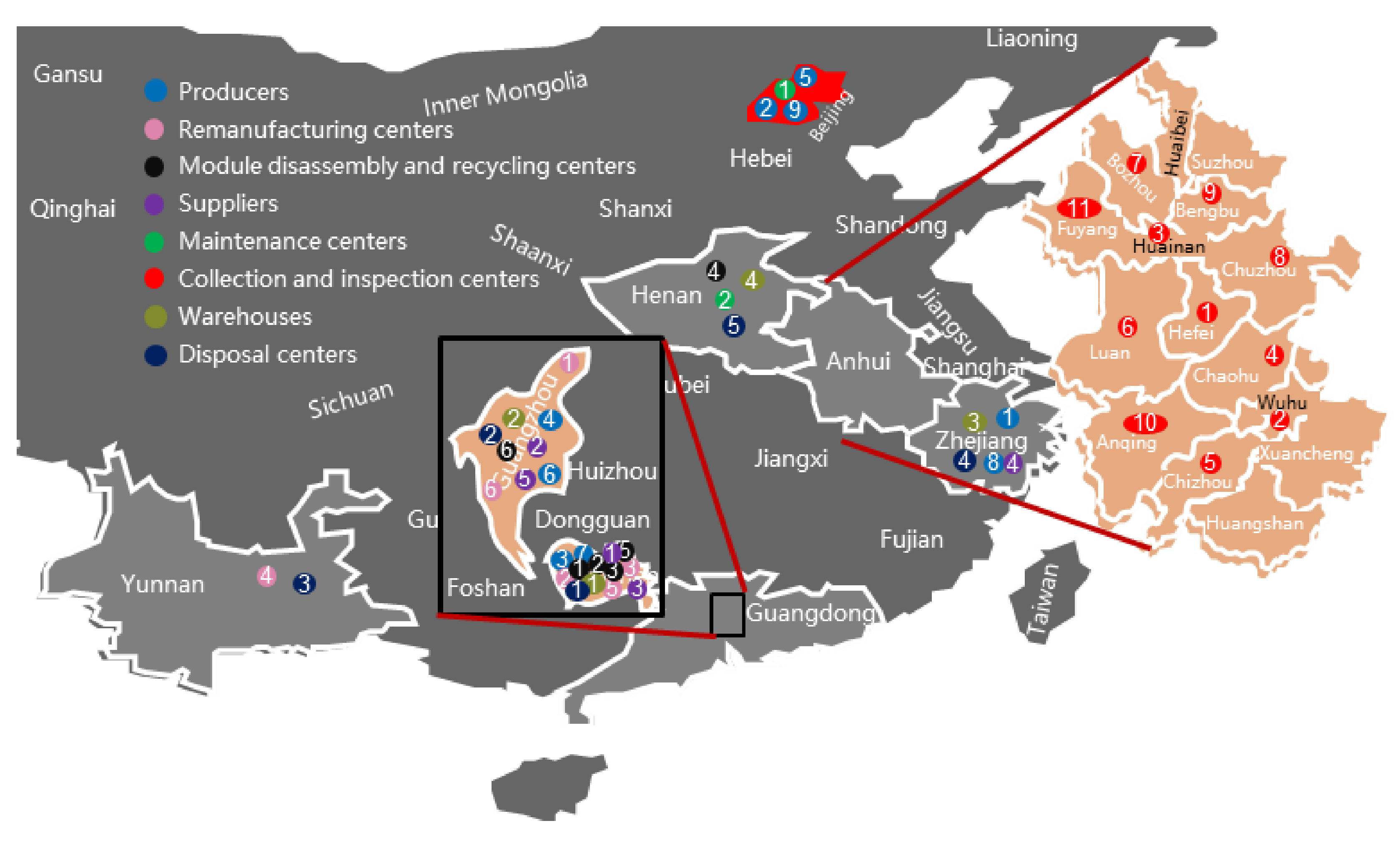
• According to the research analysis, we assume that ATMs in each city are concentrated in the warehouse as a collection and inspection center (C);
• Information on several safer warehouses (W) is determined based on the geographic location of producers (P);
• Several waste disposal centers (D) in Shenzhen, Guangzhou, Hangzhou, and Zhengzhou were selected;
• Some cost-related parameters are described in

  Table 4. Cost, carbon emissions, and capacity limit data of each company.

  Logistics Node Type	No.	Processing Cost (Unit: 1000 CNY/Piece)	Opening Cost (Unit: 1000 CNY/Period)	Carbon Emission (Unit: kg/Piece)	Capacity Limit (Upper, Lower)
  Producers	1	1.91	9.13	0.53	(7100, 3000)
  	2	1.89	14.15	0.35	(7800, 3000)
  	3	2.29	10.72	0.35	(6600, 3000)
  	4	1.51	9.83	0.43	(4100, 3000)
  	5	1.55	12.16	0.61	(7300, 3000)
  	6	2.41	10.15	0.42	(7700, 3000)
  	7	2.35	10.98	0.62	(6700, 3000)
  	8	2.01	10.19	0.35	(7000, 3000)
  	9	1.32	14.34	0.65	(6900, 3000)
  Remanufacturing centers	1	1.23	7.31	0.42	(3100, 500)
  	2	1.99	6.59	0.35	(3700, 500)
  	3	2.12	6.65	0.41	(2500, 500)
  	4	1.08	5.87	0.52	(4100, 500)
  	5	2.17	6.93	0.45	(2000, 500)
  	6	1.44	7.09	0.43	(2800, 500)
  Module disassembly and recycling centers	1	0.36	6.34	0.61	(2100, 500)
  	2	0.34	6.27	0.52	(2300, 500)
  	3	0.34	6.27	0.53	(4400, 500)
  	4	0.28	5.78	0.65	(4000, 500)
  	5	0.35	6.46	0.43	(2900, 500)
  	6	0.28	6.54	0.61	(4800, 500)
  Suppliers	1	0.06	3.88	0.63	(2100, 800)
  	2	0.07	4.05	0.46	(3300, 800)
  	3	0.06	3.91	0.52	(3100, 800)
  	4	0.09	4.72	0.33	(4300, 800)
  	5	0.07	4.04	0.31	(4400, 800)
  Maintenance centers	1	1.25	4.01	0.52	(16,000, 1500)
  	2	0.78	2.81	0.61	(16,000, 1500)
  Collection and inspection centers	1	0.67	3.08	/	(4000, 400)
  	2	0.62	2.51	/	(4100, 400)
  	3	0.53	2.76	/	(4200, 400)
  	4	0.57	2.67	/	(2800, 400)
  	5	0.45	2.51	/	(4000, 400)
  	6	0.67	2.83	/	(3900, 400)
  	7	0.39	2.52	/	(2500, 400)
  	8	0.64	2.61	/	(2300, 400)
  	9	0.39	2.82	/	(3500, 400)
  	10	0.48	2.41	/	(4800, 400)
  	11	0.61	2.51	/	(3000, 400)
  Warehouses	1	/	2.08	/	(8000, 800)
  	2	/	2.84	/	(6100, 800)
  	3	/	2.19	/	(8700, 400)
  	4	/	1.51	/	(6200, 400)
  Disposal centers	1	0.003	2.14	32	(Inf, 300)
  	2	0.001	2.09	25	(Inf, 300)
  	3	0.001	1.95	48	(Inf, 300)
  	4	0.004	2.64	31	(Inf, 300)
  	5	0.002	2.67	39	(Inf, 300)

  . These parameters make assumptions and treatments to protect the interests of merchants and are not true;
• According to the literature [4,45,46] there are established carbon emission indicators, see Table 4 column 5;
• We estimated a capacity limit based on actual production capacity and opening costs, see Table 4 column 6;
• According to the carbon emission tax reference coefficient and average vehicle load, the carbon emission coefficients of gasoline-fueled vehicles (medium-sized long-haul truck) are as follows: CT₁ = 48 g/(km*piece), CT₂ = 9 g/(km*piece);
• According to market price, we determined the following transportation costs: T1 = 15 CNY/(km*piece), T2 = 3 CNY/(km*piece);
• The distance between logistics nodes was obtained through the navigation distance of Gaode map, see Appendix A (

  Table A2. Distance from collection and inspection centers to remanufacturing center, module disassembly, recycling, and disposal centers (unit: kilometers).

  	r = 1	r = 2	r = 3	r = 4	r = 5	r = 6	l = 1	l = 2	l = 3	l = 4	l = 5	l = 6	d = 1	d = 2	d = 3	d = 4	d = 5
  c = 1	1209.5	1239.2	1240.2	1926.6	1231.7	1222.3	1249.1	1275.1	1260.8	577.8	1257.5	1239.6	1258.6	1207.5	2016.3	390.1	572.0
  c = 2	1261.6	1279.8	1280.8	2024.9	1272.7	1275.4	1289.7	1284.1	1267.3	708.5	1278.3	1272.5	1273.8	1240.4	2041.9	266.5	703.2
  c = 3	1310.3	1340.3	1341.4	1980.2	1333.2	1324.0	1350.3	1357.9	1331.6	505.2	1342.7	1314.6	1331.9	1292.8	2064.7	496.5	499.8
  c = 4	1335.5	1340.2	1341.3	2056.7	1332.7	1348.9	1350.2	1383.8	1328.4	683.8	1368.6	1350.7	1335.0	1307.7	2141.6	307.5	676.8
  c = 5	1079.1	1097.2	1098.3	1842.4	1090.1	1092.8	1107.2	1102.4	1085.6	749.2	1102.9	1090.8	1092.2	1058.8	1860.2	384.2	743.9
  c = 6	1196.3	1232.9	1227.0	1852.2	1225.8	1216.5	1242.4	1238.6	1224.2	519.3	1235.3	1207.2	1224.5	1225.5	1936.8	484.9	514.0
  c = 7	1439.9	1473.4	1470.7	2018.8	1466.3	1457.0	1480.0	1238.6	1464.7	280.1	1475.8	1447.7	1476.9	1471.2	2045.6	681.2	274.6
  c = 8	1343.6	1358.7	1359.3	2050.0	1351.6	1342.3	1368.6	1377.6	1351.3	618.5	1362.4	1344.5	1363.5	1312.4	2135.6	330.0	618.7
  c = 9	1385.5	1382.8	1383.4	2040.5	1375.7	1366.4	1392.7	1409.8	1383.6	474.4	1394.6	1376.7	1395.7	1344.6	2143.5	462.3	469.2
  c = 10	1112.9	1104.7	1105.4	1848.6	1097.2	1099.8	1113.0	1109.4	1098.8	735.7	1103.7	1097.4	1099.1	1065.7	1867.2	397.5	728.8
  c = 11	1362.1	1364.4	1365.0	1936.3	1357.3	1348.0	1383.1	1388.6	1362.3	354.3	1373.4	1345.3	1374.5	1323.4	2016.5	612.2	349.0

  ,

  Table A3. Distance from module disassembly and recycling centers to disposal centers, suppliers, and maintenance centers (unit: kilometers).

  	d = 1	d = 2	d = 3	d = 4	d = 5	s = 1	s = 2	s = 3	s = 4	s = 5	m = 1	m = 2
  l = 1	27.6	124.8	1442.1	1321.4	1539.6	12.4	112.1	10.6	1258.5	103.2	2245.3	1573.5
  l = 2	14.2	106.9	1423.8	1268.0	1546.6	5.7	91.5	25.2	1254.5	87.8	2223.7	1551.8
  l = 3	29.4	124.7	1447.0	1253.3	1544.2	25.7	114.7	20.5	1238.5	105.8	2184.2	1549.5
  l = 4	1550.4	1462.7	1968.3	928.2	24.5	1558.2	1480.8	1566.7	940.5	1479.8	701.3	0.0
  l = 5	35.9	131.3	1450.9	1262.3	1552.9	21.8	118.6	4.6	1247.5	109.7	2192.9	1558.2
  l = 6	95.2	42.0	1339.1	1256.5	1464.8	110.8	12	125.7	1241.7	23.9	2139.5	1467.7

  ,

  Table A4. Distance from producers to remanufacturing centers, supplier, and warehouses (unit: kilometers).

  	r =1	r =2	r =3	r =4	r =5	r =6	s =1	s =2	s =3	s =4	s =5	w = 1	w = 2	w = 3	w = 4
  p = 1	1253.5	1260.1	1277.2	2168.6	1282.2	1251.2	66.6	1303.4	1262.8	8.3	1238.2	1238.7	1255.1	33.1	1273.4
  p = 2	2156.0	2169.6	2185.2	2544.8	2173.5	2142.0	2189.3	2187.1	2160.1	1278.9	2134.3	2152.1	2146.9	1285.5	23.8
  p = 3	68.9	11.4	25.1	1413.5	28.0	63.1	5.7	5.7	25.5	1276.6	87.8	43.5	70.5	1318.9	2230.3
  p = 4	24.9	82.5	106.0	1360.6	99.6	20.5	92.1	92.1	106.9	1255.8	0.0	124.9	28.0	1295.7	2153.7
  p = 5	2152.0	2176.2	2191.8	2594.5	2175.9	2150.8	2196.5	2196.5	2167.8	1283.8	2139.9	2159.0	2154.7	1288.0	14.6
  p = 6	20.1	87.5	106.2	1363.5	96.5	17.9	84.7	84.7	107.1	1245.0	7.3	124.9	21.6	1290.2	2161.6
  p = 7	94.9	32.5	7.2	1447.9	31.5	92.8	23.0	23.0	3.6	1259.1	118.0	36.7	96.4	1333.1	2196.0
  p = 8	1248.4	1247.7	1248.2	2145.2	1270.5	1238.7	1267.0	1290.9	1250.3	4.8	1225.7	1227.0	1242.6	39.6	1283.6
  p = 9	2163.1	2180.2	2182.5	2551.9	2183.4	2158.1	2203.9	94.7	2171.5	1287.5	2145.5	2162.6	2157.9	1296.9	8.6

  and

  Table A5. Distance from maintenance to remanufacturing centers (unit: kilometers).

  	r = 1	r = 2	r = 3	r = 4	r = 5	r = 6
  m = 1	2164.5	2237.0	2230.0	2630.0	2225.9	2162.0
  m = 2	1492.6	1565.1	1558.1	1932.3	1554.1	1490.2

  );

5.2. Results and Discussions

This study aims to reduce the number of existing ATMs annually until the future demand for them has been met. We collected extensive data and used LINGO 12.0 to solve the proposed MILP model for RL_ATMs. LINGO shows that the model contains 508 integer variables (96 non-linear), 187 constraints (49 non-linear), and the solver type is B-and-B. Let (PEdc, PErc, PElc) = (0.2, 0.5, 0.3), (PEmo, PEco) = (0.2, 0.4), (PEdl, PEml, PEsl) = (0.1, 0.4, 0.5), and (PEpr, PEmr) = (0.8, 0.2). Moreover, the global optimal solution obtained after 7672 iterations (elapsed runtime: 17 s) is CNY 106.341 million using a PC with an Intel(R) Core (TM) i5-9300H CPU @ 2.40 GHz, with 8.0 G of RAM, of which the transportation cost is CNY 69.669 million, the transportation carbon emission is 8991 kg, the processing cost is CNY 31.094 million, and the processing carbon emission is 130,459 kg. After converting carbon emissions into RMB with a carbon tax coefficient (Con = 40 CNY/kg), the relationship between various costs is shown in Figure 6. The distribution result of each logistics node is shown in Figure 7.

The surprising aspect of the data shown in Figure 6 is that transportation costs account for 65.51% of the total costs. This result is related to the fact that several manufacturers and remanufacturers are not located in Anhui Province, and extremely long distances incur large transportation costs. If remanufacturing companies (R) and module disassembly and recycling companies (L) can be concentrated in Anhui Province, then the government would have substantial financial savings.

Figure 7 shows that out of the nine manufacturers we surveyed, only three were selected: Guangzhou Guangdian Express Financial Electronics Co., Ltd. (p = 6), Shenzhen Yihua Computer Co., Ltd. (p = 7), and Fujitsu (China) Co., Ltd. (p = 9). When p = 6, the remanufactured ATM (re-ATM) output is 6101 units; when p = 7, the re-ATM output is 3495 units; and when p = 9, the re-ATM output is 2489 units. In addition, some companies in the model have reached their capacity limits, such as r = 2, c = 5, and w = 2. The capacity of the maintenance center is 11,664 units, which represents the internal flow of the small closed loop formed by O and M. Lastly, only two out of the five disposal centers are selected under the condition that the upper limit of the capacity is infinite.

5.3. Sensitivity Analysis

5.3.1. The Impact of Capacity Changes on Total Cost

In this section, we discuss the relationship between capacity change and total cost. Taking the basic parameters of Section 5.2 as an example, the capacity of each collection and inspection center was gradually increased to eight times, and the relationship between the total cost and the capacity of the collection center is shown in

Table 5. Sensitivity analysis for the capacity of collection and inspection center.

Enlargement Factor	Total Cost	c = 1	c = 2	c = 3	c = 4	c = 5	c = 6	c = 7	c = 8	c = 9	c = 10	c = 11
×1.0	↑106.341	0	3240	0	0	4000	1730	2430	0	0	4800	0
×1.5	↑104.280	0	3240	0	0	6000	0	2430	0	0	4530	0
×2.0	↑104.238	0	3240	0	0	8000	0	2430	0	0	2530	0
×2.5	↑103.764	0	3240	0	0	10,000	0	2430	0	0	530	0
×3.0	↑102.562	0	3240	0	0	10,530	0	2430	0	0	0	0
×3.5	102.562	0	3240	0	0	10,530	0	2430	0	0	0	0
×4.0	102.562	0	3240	0	0	10,530	0	2430	0	0	0	0
×6.0	102.562	0	3240	0	0	10,530	0	2430	0	0	0	0
×8.0	102.562	0	3240	0	0	10,530	0	2430	0	0	0	0

. As shown in the table, with the expansion of capacity, the total cost gradually reduced, when the capacity expanded to more than three times the total cost, the total cost remained unchanged at CNY 102.562 million. A possible reason for this is the fact that each city can collect a limited number of ATMs, and the location of a reasonable collection center has been determined, even if its capacity is large enough, it cannot change the total number of ATMs it can collect. Similarly, the ATMs collected by c = 2 and c = 7 are always the same at 3240 and 2430, respectively. In addition, we can see that the number of ATMs that can be collected by c = 5 collection centers is always equal to its capacity ceiling until the number of ATMs that can be collected by c = 6 and c = 10 is reduced to zero. Lastly, when the capacity of the C centers expands indefinitely, the total cost is fixed at 102.562 million yuan. The number of ATMs collected for c = 2, c = 5, and c = 7 converges to: 3240, 10,530, and 2430, respectively.

We separately analyzed the situation of other logistics nodes, and the relationship between the size of the capacity and the total cost is shown in Figure 8. In Figure 8, when the capacity of W is increased to 3.5 times and the capacity of M is increased to 4 times, the smallest total cost can be obtained, which are 102.426 million yuan and 102.445 million yuan, respectively. On the contrary, increasing the capacity of L does not significantly reduce the total cost, which is closely related to the elimination of ATMs and the relative position between logistics nodes. In addition, when the capacity of D is expanded to 5 times, the total cost decreases, and finally decreases to 104.236 million yuan. Overall, increasing the capacity of logistics nodes will make the total cost of RL_ATMs smaller. However, when considering the constraints such as the convenience of management, the availability of capacity and the convenience of delivery, it needs to be comprehensively considered to achieve the best planning results.

Figure 8. Sensitivity analysis for the capacity.

Figure 8. Sensitivity analysis for the capacity.

5.3.2. Relation between the Value of PE and the Objective Function

In the RL_ATMs model, the total production of each level is determined by the percentage diversion method, and the ratio coefficient of distribution is an important parameter of the method. Therefore, the relationship between the value of PE and objective function should be discussed.

Table 6 presents 22 results based on different diversion ratio coefficients: collection and inspection centers (C) and maintenance centers (M) account for the percentage of operators (O) in logistics quantity; disposal centers (D), remanufacturing centers (R), and module disassembly and recycling centers (L) account for the percentage of collection and inspection centers (C) in logistics quantity. Columns 2 to 5 in Table 6 represent different diversion proportional coefficients, and column 6 indicates the number of periods over which ATM holdings can be made to match the projected number of requirements. Column 7 is the ATM traffic in the closed loop formed by M and O. We used the processing capacity Nm of the maintenance center to represent it. Columns 8 to 10 show the result of the objective function, where CF is the cost function and EF is the environmental emission function. The effect of each parameter change on the result is discussed separately in conjunction with Table 6:

• In contrast to cases 1, 2, and 3, as PEco increases, the number of ATM recycling and decommissioning per period increases, the number of periods required to meet the projected market holding requirements decreases, and the cost decreases; however, carbon tax increases. Comparing cases 1 and 3, although carbon tax only increased by CNY 0.515 million, it emits 12,875 kg of CO₂. In addition, the increase in PEco leads to a decrease in Nm;
• Comparing cases 2, 4, and 5, the increase in PEmo has no effect on the number of periods, but carbon tax and cost evidently increased. This research does not consider the economic profit that can be provided by upgraded ATMs. However, the actual data indicated that if PEmo is added, then the economic benefits of the model may be improved because the processing capacity of the maintenance center increases;
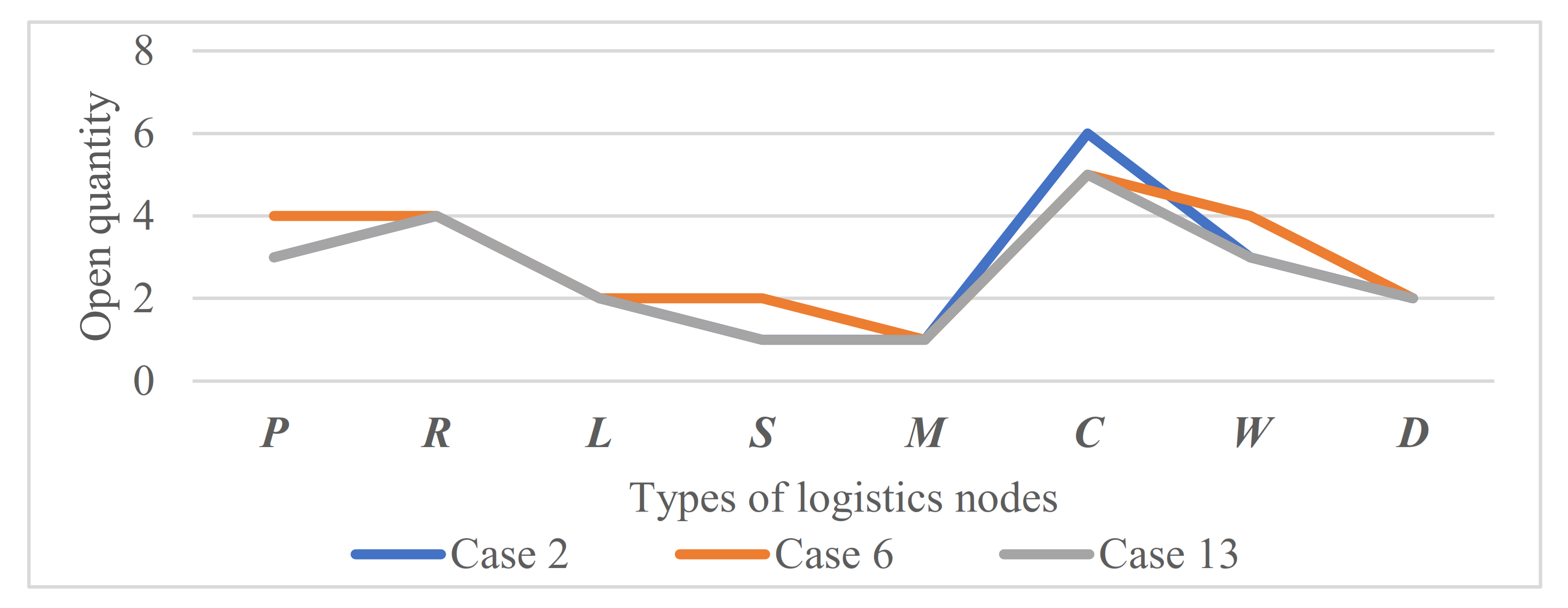
• Cases 2, 6, and 7 indicate that keeping the processing ratio PEdc unchanged, when the remanufacturing ratio PElc increases and module disassembly recycling ratio PErc reduces, the period and cost decreases, but carbon tax changes irregularly;
• By analyzing cases 7, 8, and 9, period and cost are reduced under the conditions that PErc is constant, PEdc has been added, and PElc has been reduced. Evidently, this waste of resources increases from case 7 to 9, which also has the largest carbon tax collection of the 22 cases in Table 6. In addition, an increase in PEdc will cause Nm to decrease;
• In cases 9, 10, and 11, period and costs were reduced with PElc unchanged, PEdc increased, and PErc decreased, similar to the results of the previous analysis (i.e., No. 4). Given that the original intent of the RL_ATMs model is to recycle ATMs as much as possible, PErc > PElc should be satisfied. Moreover, the smaller the PEdc, the better;
• Through the analysis of case 6 and case 12–17, the smaller the PEdl, the lower the carbon tax, the more beneficial to the environment. The value of PEml is related to the replacement rate of parts and components between new and old ATMs. Hence, The larger the PEml value, the lower the cost;
• Combining case 13 and cases 18–22 for analyses: changes in PEpr and PEmr have no effect on the period. Moreover, the pattern of impact on costs and Nm is difficult to determine. However, the carbon tax is gradually decreasing.

Table 6. Case and solutions.

No.	Diversion from O	Diversion from C	Diversion from L	Diversion from R	Period	Nm	Objective Function (Unit: CNY million)
	(PEmo, PEco)	(PEdc, PErc, PElc)	(PEdl, PEml, PEsl)	(PEpr, PEmr)			CF	EF	Total
Case 1	(0.2,0.3)	(0.2,0.6,0.2)	(0.1,0.2,0.7)	(0.8,0.2)	6	14649	130.335	5.899	136.234
Case 2	(0.2,0.4)	(0.2,0.6,0.2)	(0.1,0.2,0.7)	(0.8,0.2)	5	12,882	127.554	6.401	133.955
Case 3	(0.2,0.5)	(0.2,0.6,0.2)	(0.1,0.2,0.7)	(0.8,0.2)	4	11,033	119.931	6.414	126.345
Case 4	(0.3,0.4)	(0.2,0.6,0.2)	(0.1,0.2,0.7)	(0.8,0.2)	5	17,761	156.241	6.509	162.750
Case 5	(0.4,0.4)	(0.2,0.6,0.2)	(0.1,0.2,0.7)	(0.8,0.2)	5	22,640	201.34	6.589	207.929
Case 6	(0.2,0.4)	(0.2,0.5,0.3)	(0.1,0.2,0.7)	(0.8,0.2)	4	10,692	102.075	5.596	107.671
Case 7	(0.2,0.4)	(0.2,0.4,0.4)	(0.1,0.2,0.7)	(0.8,0.2)	4	10,627	98.645	5.838	104.483
Case 8	(0.2,0.4)	(0.3,0.4,0.3)	(0.1,0.2,0.7)	(0.8,0.2)	3	7807	75.759	5.683	81.442
Case 9	(0.2,0.4)	(0.4,0.4,0.2)	(0.1,0.2,0.7)	(0.8,0.2)	3	7283	73.346	6.838	80.184
Case 10	(0.2,0.4)	(0.5,0.3,0.2)	(0.1,0.2,0.7)	(0.8,0.2)	2	5004	52.675	5.744	58.419
Case 11	(0.2,0.4)	(0.6,0.2,0.2)	(0.1,0.2,0.7)	(0.8,0.2)	2	4729	51.532	6.83	58.362
Case 12	(0.2,0.4)	(0.2,0.5,0.3)	(0.1,0.3,0.6)	(0.8,0.2)	4	11,178	100.945	5.59	106.535
Case 13	(0.2,0.4)	(0.2,0.5,0.3)	(0.1,0.4,0.5)	(0.8,0.2)	4	11,664	100.763	5.578	106.341
Case 14	(0.2,0.4)	(0.2,0.5,0.3)	(0.2,0.4,0.4)	(0.8,0.2)	4	11,453	95.944	6.199	102.143
Case 15	(0.2,0.4)	(0.2,0.5,0.3)	(0.3,0.4,0.3)	(0.8,0.2)	4	11,245	92.82	6.794	99.614
Case 16	(0.2,0.4)	(0.2,0.5,0.3)	(0.4,0.3,0.3)	(0.8,0.2)	3	8453	72.52	5.877	78.397
Case 17	(0.2,0.4)	(0.2,0.5,0.3)	(0.5,0.2,0.3)	(0.8,0.2)	3	7984	71.77	6.361	78.131
Case 18	(0.2,0.4)	(0.2,0.5,0.3)	(0.1,0.4,0.5)	(0.7,0.3)	4	12,474	102.085	5.573	107.658
Case 19	(0.2,0.4)	(0.2,0.5,0.3)	(0.1,0.4,0.5)	(0.6,0.4)	4	13,284	105.408	5.575	110.983
Case 20	(0.2,0.4)	(0.2,0.5,0.3)	(0.1,0.4,0.5)	(0.5,0.5)	4	14,094	108.656	5.557	114.213
Case 21	(0.2,0.4)	(0.2,0.5,0.3)	(0.1,0.4,0.5)	(0.4,0.6)	4	14,904	108.306	5.536	113.842
Case 22	(0.2,0.4)	(0.2,0.5,0.3)	(0.1,0.4,0.5)	(0.3,0.7)	4	15,714	120.378	5.551	125.929

Table 6. Case and solutions.

No.	Diversion from O	Diversion from C	Diversion from L	Diversion from R	Period	Nm	Objective Function (Unit: CNY million)
	(PEmo, PEco)	(PEdc, PErc, PElc)	(PEdl, PEml, PEsl)	(PEpr, PEmr)			CF	EF	Total
Case 1	(0.2,0.3)	(0.2,0.6,0.2)	(0.1,0.2,0.7)	(0.8,0.2)	6	14649	130.335	5.899	136.234
Case 2	(0.2,0.4)	(0.2,0.6,0.2)	(0.1,0.2,0.7)	(0.8,0.2)	5	12,882	127.554	6.401	133.955
Case 3	(0.2,0.5)	(0.2,0.6,0.2)	(0.1,0.2,0.7)	(0.8,0.2)	4	11,033	119.931	6.414	126.345
Case 4	(0.3,0.4)	(0.2,0.6,0.2)	(0.1,0.2,0.7)	(0.8,0.2)	5	17,761	156.241	6.509	162.750
Case 5	(0.4,0.4)	(0.2,0.6,0.2)	(0.1,0.2,0.7)	(0.8,0.2)	5	22,640	201.34	6.589	207.929
Case 6	(0.2,0.4)	(0.2,0.5,0.3)	(0.1,0.2,0.7)	(0.8,0.2)	4	10,692	102.075	5.596	107.671
Case 7	(0.2,0.4)	(0.2,0.4,0.4)	(0.1,0.2,0.7)	(0.8,0.2)	4	10,627	98.645	5.838	104.483
Case 8	(0.2,0.4)	(0.3,0.4,0.3)	(0.1,0.2,0.7)	(0.8,0.2)	3	7807	75.759	5.683	81.442
Case 9	(0.2,0.4)	(0.4,0.4,0.2)	(0.1,0.2,0.7)	(0.8,0.2)	3	7283	73.346	6.838	80.184
Case 10	(0.2,0.4)	(0.5,0.3,0.2)	(0.1,0.2,0.7)	(0.8,0.2)	2	5004	52.675	5.744	58.419
Case 11	(0.2,0.4)	(0.6,0.2,0.2)	(0.1,0.2,0.7)	(0.8,0.2)	2	4729	51.532	6.83	58.362
Case 12	(0.2,0.4)	(0.2,0.5,0.3)	(0.1,0.3,0.6)	(0.8,0.2)	4	11,178	100.945	5.59	106.535
Case 13	(0.2,0.4)	(0.2,0.5,0.3)	(0.1,0.4,0.5)	(0.8,0.2)	4	11,664	100.763	5.578	106.341
Case 14	(0.2,0.4)	(0.2,0.5,0.3)	(0.2,0.4,0.4)	(0.8,0.2)	4	11,453	95.944	6.199	102.143
Case 15	(0.2,0.4)	(0.2,0.5,0.3)	(0.3,0.4,0.3)	(0.8,0.2)	4	11,245	92.82	6.794	99.614
Case 16	(0.2,0.4)	(0.2,0.5,0.3)	(0.4,0.3,0.3)	(0.8,0.2)	3	8453	72.52	5.877	78.397
Case 17	(0.2,0.4)	(0.2,0.5,0.3)	(0.5,0.2,0.3)	(0.8,0.2)	3	7984	71.77	6.361	78.131
Case 18	(0.2,0.4)	(0.2,0.5,0.3)	(0.1,0.4,0.5)	(0.7,0.3)	4	12,474	102.085	5.573	107.658
Case 19	(0.2,0.4)	(0.2,0.5,0.3)	(0.1,0.4,0.5)	(0.6,0.4)	4	13,284	105.408	5.575	110.983
Case 20	(0.2,0.4)	(0.2,0.5,0.3)	(0.1,0.4,0.5)	(0.5,0.5)	4	14,094	108.656	5.557	114.213
Case 21	(0.2,0.4)	(0.2,0.5,0.3)	(0.1,0.4,0.5)	(0.4,0.6)	4	14,904	108.306	5.536	113.842
Case 22	(0.2,0.4)	(0.2,0.5,0.3)	(0.1,0.4,0.5)	(0.3,0.7)	4	15,714	120.378	5.551	125.929

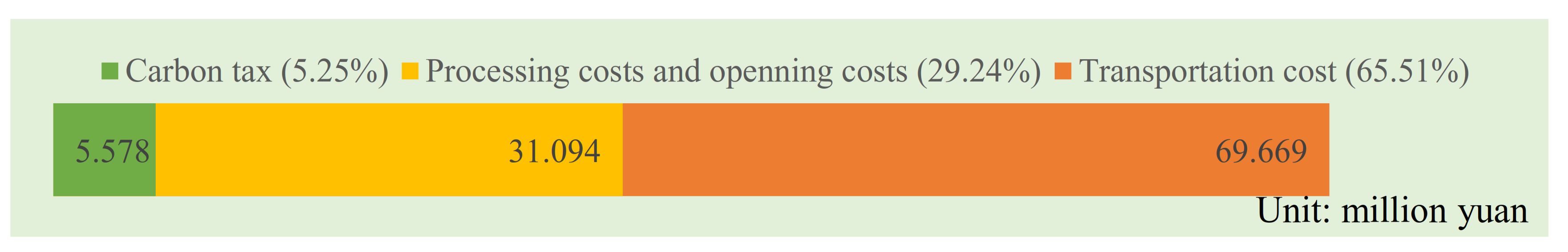
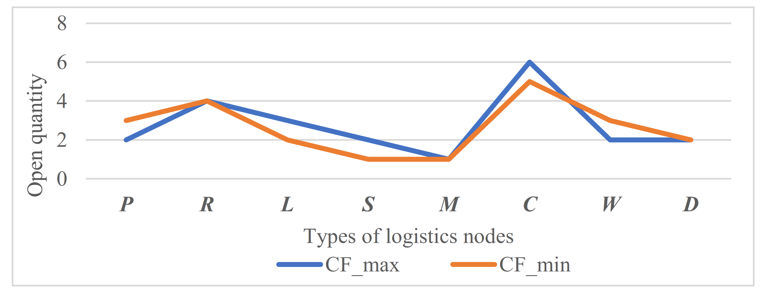
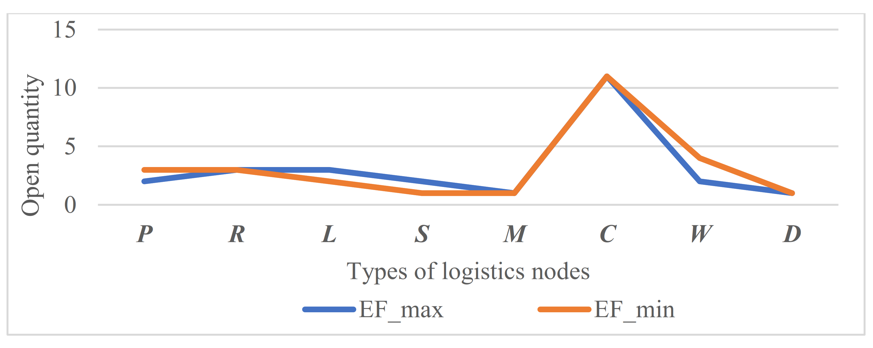
5.3.3. Cost and Environmental Analysis

In this study, cost function is composed of the opening cost of each logistics node, the dismantling cost of ATMs and their module remanufacturing cost, and transportation cost. The environmental emission function is composed of carbon emissions from transportation, module disassembly and processing, and waste disposal. On the basis of the diversion coefficient of case 13, the minimum (maximum) value of CF in the case of neglecting the environmental emission function and minimum (maximum) value of EF in the case of neglecting the cost function were obtained (Table 7). The “type of logistics node” in the right column of Table 7 lists the index number of the selected logistics node.

Figure 9 shows the distribution of the number of open logistics nodes corresponding to the maximum and minimum values of CF [22]. By contrast, except for P, R, M, and W, the open numbers of all other logistics nodes are 1 more when CF reaches its maximum than when CF reaches its minimum. Moreover, the open numbers of R and M are equal. Therefore, the open quantity of M and R is not the main decisive factor when considering only the cost. To increase the state’s support to technology-based companies, open quantity can be increased moderately.

Table 7. Maximum and minimum of CF and EF.

	Objective Function (RMB: CNY Million)		Type of Logistics Node
	CF	EF	P	R	L	S	M	C	W	D
max	621.178	/	5, 9	1, 2, 3, 5	1,2,4	1, 3	1	4, 5, 7, 8, 9, 11	1, 2	3, 5
min	97.476	/	6, 7, 9	1, 3, 5, 6	4, 6	2	2	2, 5, 6, 7, 10	1, 2, 4	4, 5
max	/	8.044	7, 9	4, 5, 6	1, 4, 6	1, 3	2	1, 2, 3, 4, 5, 6, 7, 8, 9, 10, 11	1, 2	3
min	/	4.374	2, 3, 8	1, 2, 3	2, 5	5	1	1, 2, 3, 4, 5, 6, 7, 8, 9, 10, 11	1, 2, 3, 4	1

Table 7. Maximum and minimum of CF and EF.

	Objective Function (RMB: CNY Million)		Type of Logistics Node
	CF	EF	P	R	L	S	M	C	W	D
max	621.178	/	5, 9	1, 2, 3, 5	1,2,4	1, 3	1	4, 5, 7, 8, 9, 11	1, 2	3, 5
min	97.476	/	6, 7, 9	1, 3, 5, 6	4, 6	2	2	2, 5, 6, 7, 10	1, 2, 4	4, 5
max	/	8.044	7, 9	4, 5, 6	1, 4, 6	1, 3	2	1, 2, 3, 4, 5, 6, 7, 8, 9, 10, 11	1, 2	3
min	/	4.374	2, 3, 8	1, 2, 3	2, 5	5	1	1, 2, 3, 4, 5, 6, 7, 8, 9, 10, 11	1, 2, 3, 4	1

Figure 10 presents the distribution of the open number of logistics nodes corresponding to the maximum and minimum values of EF. By contrast, the maximum of EF is compared with the minimum, the open numbers of L and S are more, and the open numbers of P and W are less. Data in Table 4 show that P’s carbon emissions are lower than those of other types of logistics nodes. In addition, the assumption is that ATMs do not generate carbon emissions when stored in warehouses.

Figure 11 shows the distribution of the open number of logistics nodes corresponding to cases 2, 6, and 13. Table 6 shows that the objective function values of the three cases are reduced. Compared with case 6, case 2 has more C and less W, and case 6 has more P, S, and W than case 13. Therefore, the open numbers of P, S, C, and W have a substantial impact on the total cost.

The following assumes that the objective function of the model is: ${\omega }_1•CF+{\omega }_2•EF•Con,\mathrm{Total} \mathrm{cost}= CF+EF•Con$ and ${\omega }_1+{\omega }_2=1$. We analyze the relationship between CF and EF, Total cost and EF, respectively.

The different values of ω₁ are taken from small to large, and the result obtained is shown in Figure 12. Only when the value of ω₁ is between 0.05 and 0.20 can the values of CF and EF change. In other cases, CF = 129.198 (Total cost = 134.098) million CNY and EF = 5.900 million CNY are maintained. Therefore, the value of ω₁ has minimal effect on the final optimization result of the model. This is consistent with the conclusion drawn in the literature [15,47]. Their research results indicated that the reduction in economic costs inevitably leads to an increase in carbon emissions. However, the results in Figure 12 show that the two can obtain balanced optimization results.

6. Conclusions

In recent years, the use frequency and transaction volume of mobile payments have increased significantly, thereby decreasing people’s demand for cash and banks’ demand for ATMs. In China, this phenomenon is particularly prominent. This study combines the four processing methods of decommissioned ATMs and proposes a reverse logistics model with minimal cost and environmental emissions. Moreover, a simulation solution is provided on the basis of the basic situation in Anhui Province, China. The RL_ATMs model comprises suppliers, producers, warehouses, operators, maintenance centers, collection and inspection centers, disposal centers, remanufacturing centers, and recycling centers (i.e., nine levels). ATMs comprise a planned and batch process from launch to decommissioning. Therefore, the percentage diversion method is proposed to convert a multi-period problem into a single-period problem. Accordingly, the complexity of the solution process is reduced. Lastly, the RL_ATMs model is expressed as a MILP model and solved using LINGO 12.0.

According to the analysis of the solution result of case 13 (i.e., in Table 6), which is the most consistent with the actual situation, the total cost includes 65.51%, 29.24%, and 5.25% of the transportation cost, operating cost, and carbon tax, respectively. In this case, the transportation cost accounts for a large proportion because some manufacturers, remanufacturing centers, and dismantling centers are not located in Anhui Province. Meanwhile, carbon tax accounts for a relatively small proportion, which is related to China’s environmental emission policy.

The sensitivity analysis scheme is set according to the change of the percentage parameter (PE) of the percentage transfer method, as shown in Table 6, a total of 22. The comparative analyses conducted concluded their influence on the objective function and period and the M-O closed-loop influence relationship. In actual applications, it should be set according to the relevant technical level and economic input. In the link of cost and environment analyses, this research concludes that the open number of remanufacturing and maintenance centers has minimal effects on the cost function. If the development of technology-based enterprises is necessary, their open number can be increased.

Although the calculation results in this study are similar to our survey results, there will definitely be deviations from the calculation results after the project enters the implementation stage. We can reduce the deviation by adjusting the value of PE or further enriching the RL_ATMs model. We considered 10 PE coefficients in the reverse logistics network design model, and analyzed their influence on the optimization results, in order to fit the actual situation. The problem that comes with it is that we cannot find the optimal value of these coefficients. However, whether these coefficients have a positive or negative impact on the results, and the degree of influence are discussed in this paper. In addition, we can also obtain the optimal network model results under the provided proportional parameters.

In the end, we can make further research through the following aspects. (1) A nonlinear model can be proposed to represent the true process of ATMs recycling and remanufacturing. For instance, the uncertainty of returns and demand. (2) As the scale of the problem increase, the complexity of the problem increases exponentially. The research of using a heuristic solution method is crucial for the improvement of problem-solving speed. (3) With the support of technology and operation means, the revenue forecast of various means of ATM disposal and when it will reach an equilibrium so that the rate of decommissioning ATMs reduces, may be an interesting research subject if the accurate ATMs ownership, scrap and relevant economic data can be obtained. In addition, we should also add other calculation goals (e.g., maximum profit and maximum social benefit) to make the calculation results consistent with the actual situation.

References

1. Fan, X.; Zhao, W.; Zhang, T.; Yan, E. Mobile payment, third-party payment platform entry and information sharing in supply chains. Ann. Oper. Res. 2020, 1–20. [Google Scholar] [CrossRef] [PubMed]
2. Qi, M.; Valverde, S.C.; Fernandez, F.R. The diffusion pattern of non-cash payments: Evidence from China. Int. J. Technol. Manag. 2016, 70, 44–57. [Google Scholar] [CrossRef]
3. Denstad, A.; Ulsund, E.; Christiansen, M.; Hvattum, L.M.; Tirado, G. Multi-objective optimization for a strategic ATM network redesign problem. Ann. Oper. Res. 2021, 296, 7–33. [Google Scholar] [CrossRef]
4. Yu, H.; Solvang, W.D. A Stochastic Programming Approach with Improved Multi-Criteria Scenario-Based Solution Method for Sustainable Reverse Logistics Design of Waste Electrical and Electronic Equipment (WEEE). Sustainability 2016, 8, 1331. [Google Scholar] [CrossRef] [Green Version]
5. Cruz-Rivera, R.; Ertel, J. Reverse logistics network design for the collection of End-of-Life Vehicles in Mexico. Eur. J. Oper. Res. 2009, 196, 930–939. [Google Scholar] [CrossRef]
6. Bernon, M.; Tjahjono, B.; Ripanti, E. Aligning retail reverse logistics practice with circular economy values: An exploratory framework. Prod. Plan. Control. 2018, 29, 483–497. [Google Scholar] [CrossRef]
7. Trochu, J.; Chaabane, A.; Ouhimmou, M. A carbon-constrained stochastic model for eco-efficient reverse logistics network design under environmental regulations in the CRD industry. J. Clean. Prod. 2020, 245, 1–16. [Google Scholar] [CrossRef]
8. Kumar, D.A.; Iniyan, B.; Askar, M.A.; Ajay, A.; Ambika, R. Face Recognition Based New Generation ATM Machine. In Proceedings of the 5th International Conference on Advanced Computing & Communication Systems (ICACCS), Coimbatore, India, 15–16 March 2019; pp. 938–943. [Google Scholar]
9. Lasisi, H.; Ajisafe, A.A. Development of Stripe Biometric Based Fingerprint Authentications Systems in Automated Teller Machines. In Proceedings of the 2nd International Conference on Advances in Computational Tools for Engineering Applications (ACTEA), Beirut, Lebanon, 12–15 December 2012; pp. 172–175. [Google Scholar] [CrossRef]
10. Šomplák, R.; Pavlas, M.; Nevrlý, V.; Touš, M.; Popela, P. Contribution to Global Warming Potential by waste producers: Identification by reverse logistic modelling. J. Clean. Prod. 2018, 208, 1294–1303. [Google Scholar] [CrossRef]
11. Guarnieri, P.; Streit, J.A.C.; Batista, L.C. Reverse logistics and the sectoral agreement of packaging industry in Brazil towards a transition to circular economy. Resour. Conserv. Recycl. 2020, 153, 104541. [Google Scholar] [CrossRef]
12. Fleischmann, M.; Bloemhof-Ruwaard, J.M.; Dekker, R.; van der Laan, E.; van Nunen, J.A.; Van Wassenhove, L.N. Quantitative models for reverse logistics: A review. Eur. J. Oper. Res. 1997, 103, 1–17. [Google Scholar] [CrossRef] [Green Version]
13. Govindan, K.; Soleimani, H. A review of reverse logistics and closed-loop supply chains: A Journal of Cleaner Production focus. J. Clean. Prod. 2017, 142, 371–384. [Google Scholar] [CrossRef]
14. Liao, T.-Y. Reverse logistics network design for product recovery and remanufacturing. Appl. Math. Model. 2018, 60, 145–163. [Google Scholar] [CrossRef]
15. Gao, X. A Novel Reverse Logistics Network Design Considering Multi-Level Investments for Facility Reconstruction with Environmental Considerations. Sustainability 2019, 11, 2710. [Google Scholar] [CrossRef] [Green Version]
16. Kannan, D.; Diabat, A.; Alrefaei, M.; Govindan, K.; Yong, G. A carbon footprint based reverse logistics network design model. Resour. Conserv. Recycl. 2012, 67, 75–79. [Google Scholar] [CrossRef]
17. Pourjavad, E.; Mayorga, R.V. An optimization model for network design of a closed-loop supply chain: A study for a glass manufacturing industry. Int. J. Manag. Sci. Eng. Manag. 2019, 14, 169–179. [Google Scholar] [CrossRef]
18. Islam, T.; Nizami, M.S.H.; Mahmoudi, S.; Huda, N. Reverse logistics network design for waste solar photovoltaic panels: A case study of New South Wales councils in Australia. Waste Manag. Res. 2021, 39, 386–395. [Google Scholar] [CrossRef]
19. Wu, D.; Huo, J.; Zhang, G.; Zhang, W. Minimization of Logistics Cost and Carbon Emissions Based on Quantum Particle Swarm Optimization. Sustainability 2018, 10, 3791. [Google Scholar] [CrossRef] [Green Version]
20. Alkhayyal, B. Corporate Social Responsibility Practices in the U.S.: Using Reverse Supply Chain Network Design and Optimization Considering Carbon Cost. Sustainability 2019, 11, 2097. [Google Scholar] [CrossRef] [Green Version]
21. Safdar, N.; Khalid, R.; Ahmed, W.; Imran, M. Reverse logistics network design of e-waste management under the triple bottom line approach. J. Clean Prod. 2020, 272, 122662. [Google Scholar] [CrossRef]
22. Aydin, N. Designing reverse logistics network of end-of-life-buildings as preparedness to disasters under uncertainty. J. Clean. Prod. 2020, 256, 120341. [Google Scholar] [CrossRef]
23. Li, Z.; Xie, C.; Peng, P.; Gao, X.; Wan, Q. Multi-objective location-scale optimization model and solution methods for large-scale emergency rescue resources. Environ. Sci. Pollut. Res. 2021, 1–14. [Google Scholar] [CrossRef]
24. Li, J.-Q.; Xue, Y.; Wang, J.-D.; Pan, Q.-K.; Duan, P.-Y.; Sang, H.-Y.; Gao, K.-Z. A hybrid artificial bee colony for optimizing a reverse logistics network system. Soft Comput. 2017, 97, 76–6018. [Google Scholar] [CrossRef]
25. Sifaleras, A.; Konstantaras, I. Variable neighborhood descent heuristic for solving reverse logistics multi-item dynamic lot-sizing problems. Comput. Oper. Res. 2017, 78, 385–392. [Google Scholar] [CrossRef]
26. Sun, W.; Su, Y. Analysing Green Forward–Reverse Logistics with NSGA-II. Sustainability 2020, 12, 6082. [Google Scholar] [CrossRef]
27. Temucin, T.; Tuzkaya, G. A multi-objective reverse logistics network design model for after-sale services and a tabu search based methodology. J. Intell. Fuzzy Syst. 2020, 38, 4139–4157. [Google Scholar] [CrossRef]
28. Kinobe, J.; Gebresenbet, G.; Niwagaba, C.; Vinneras, B. Reverse logistics system and recycling potential at a landfill: A case study from Kampala City. Waste Manag. 2015, 42, 82–92. [Google Scholar] [CrossRef] [PubMed]
29. de Oliveira, C.T.; Luna, M.M.; Campos, L.M. Understanding the Brazilian expanded polystyrene supply chain and its reverse logistics towards circular economy. J. Clean. Prod. 2019, 235, 562–573. [Google Scholar] [CrossRef]
30. Kuşakcı, A.O.; Ayvaz, B.; Cin, E.; Aydın, N. Optimization of reverse logistics network of End of Life Vehicles under fuzzy supply: A case study for Istanbul Metropolitan Area. J. Clean. Prod. 2019, 215, 1036–1051. [Google Scholar] [CrossRef]
31. Wang, Z.; Hao, H.; Gao, F.; Zhang, Q.; Zhang, J.; Zhou, Y. Multi-attribute decision making on reverse logistics based on DEA-TOPSIS: A study of the Shanghai End-of-life vehicles industry. J. Clean. Prod. 2019, 214, 730–737. [Google Scholar] [CrossRef]
32. de Campos, E.A.R.; de Paula, I.C.; Caten, C.S.T.; Maçada, A.C.G.; Marôco, J.; Ziegelmann, P.K. The effect of collaboration and IT competency on reverse logistics competency—Evidence from Brazilian supply chain executives. Environ. Impact Assess. Rev. 2020, 84, 106433. [Google Scholar] [CrossRef]
33. Tadaros, M.; Migdalas, A.; Samuelsson, B.; Segerstedt, A. Location of facilities and network design for reverse logistics of lithium-ion batteries in Sweden. Oper. Res. 2020, 1–21. [Google Scholar] [CrossRef]
34. Wijewickrama, M.; Chileshe, N.; Rameezdeen, R.; Ochoa, J.J. Quality assurance in reverse logistics supply chain of demolition waste: A systematic literature review. Waste Manag. Res. 2021, 39, 3–24. [Google Scholar] [CrossRef]
35. Kazancoglu, Y.; Ekinci, E.; Mangla, S.K.; Sezer, M.D.; Kayikci, Y. Performance evaluation of reverse logistics in food supply chains in a circular economy using system dynamics. Bus. Strat. Environ. 2021, 30, 71–91. [Google Scholar] [CrossRef]
36. Pinheiro, E.; de Francisco, A.C.; Piekarski, C.M.; de Souza, J.T. How to identify opportunities for improvement in the use of reverse logistics in clothing industries? A case study in a Brazilian cluster. J. Clean. Prod. 2019, 210, 612–619. [Google Scholar] [CrossRef]
37. Kaviani, M.A.; Tavana, M.; Kumar, A.; Michnik, J.; Niknam, R.; de Campos, E.A.R. An integrated framework for evaluating the barriers to successful implementation of reverse logistics in the automotive industry. J. Clean. Prod. 2020, 272, 122714. [Google Scholar] [CrossRef]
38. Guo, J.; Tan, R.; Sun, J.; Cao, G.; Zhang, L. An approach for generating design scheme of new market disruptive products driven by function differentiation. Comput. Ind. Eng. 2016, 102, 302–315. [Google Scholar] [CrossRef]
39. Ahmed, W.; Sarkar, B. Management of next-generation energy using a triple bottom line approach under a supply chain framework. Resour. Conserv. Recycl. 2019, 150. [Google Scholar] [CrossRef]
40. Zhu, Q.; Sarkis, J. Relationships between operational practices and performance among early adopters of green supply chain management practices in Chinese manufacturing enterprises. J. Oper. Manag. 2004, 22, 265–289. [Google Scholar] [CrossRef]
41. Vachon, S.; Klassen, R.D. Environmental management and manufacturing performance: The role of collaboration in the supply chain. Int. J. Prod. Econ. 2008, 111, 299–315. [Google Scholar] [CrossRef]
42. Mondal, P.C.; Deb, R.; Adnan, N. On reinforcing automatic teller machine (ATM) transaction authentication security process by imposing behavioral biometrics. In Proceedings of the 4th International Conference on Advances in Electrical Engineering (ICAEE), Dhaka, Bangladesh, 28–30 September 2017; pp. 369–372. [Google Scholar] [CrossRef]
43. Gaur, J.; Amini, M.; Rao, A. Closed-loop supply chain configuration for new and reconditioned products: An integrated optimization model. Omega 2017, 66, 212–223. [Google Scholar] [CrossRef]
44. Yildiz, C.; Açikgöz, H. Forecasting diversion type hydropower plant generations using an artificial bee colony based extreme learning machine method. Energy Sources Part B Econ. Plan. Policy 2021, 16, 1–19. [Google Scholar] [CrossRef]
45. Gagliardi, F.; Palaia, D.; Ambrogio, G. Energy consumption and CO2 emissions of joining processes for manufacturing hybrid structures. J. Clean. Prod. 2019, 228, 425–436. [Google Scholar] [CrossRef]
46. Jeswiet, J.; Kara, S. Carbon emissions and CESTM in manufacturing. CIRP Ann. 2008, 57, 17–20. [Google Scholar] [CrossRef]
47. Xiao, Z.; Sun, J.; Shu, W.; Wang, T. Location-allocation problem of reverse logistics for end-of-life vehicles based on the measurement of carbon emissions. Comput. Ind. Eng. 2019, 127, 169–181. [Google Scholar] [CrossRef]
Figure 1. Distribution and trend of global ATM ownership.
Sustainability 13 11373 g001
Figure 5. Location of candidate logistics nodes. Different colors represent different types of logistics nodes, and numbers represent the index of logistics nodes (corresponding to Table A1).
Sustainability 13 11373 g005
Figure 6. Quantity of each cost and its percentage in the total cost.
Sustainability 13 11373 g006
Figure 7. An optimization solution based on LINGO.
Sustainability 13 11373 g007
Figure 9. Maximum (minimum) CF corresponds to the open number of logistics nodes.
Sustainability 13 11373 g009
Figure 10. Maximum (minimum) EF corresponds to the open number of logistics nodes.
Sustainability 13 11373 g010
Figure 11. Case 2, 6 and 13 correspond to the open number of logistics nodes.
Sustainability 13 11373 g011
Figure 12. Effect of the objective function on the value of ω1.
Sustainability 13 11373 g012