Identification of the Relative Importance of Factors Affecting the Spatial Variability of River Water Quality

Abstract

Understanding the temporal and spatial variability of water quality is important in order to establish effective customized management strategies for polluted aquatic ecosystems. Although various water quality management methods have been proposed based on insights into river water pollution factors through physically based modeling or statistical techniques, it is difficult to find studies that analyze the relative importance of these water pollution factors in a relatively large watershed using a step-by-step methodology. In this study, the spatial variability of river water quality is analyzed using time-averaged river water quality data collected from 40 sites in the Nakdong river basin, located on the Korean Peninsula. We focused on biological oxygen demand, total suspended solids, total nitrogen, and total organic carbon. A two-step exhaustive search approach was used to find a linear model that best links the various factors of the watershed with the average river water quality. The optimal model was selected by applying cross-correlation analysis and Bayesian inference. Through the process of finding the optimal statistical model, the major factors that have the most influence on river water quality were identified by analyzing the factors affecting river water quality, their levels of influence, and their levels of uncertainty. Identifying a set of processes provides insight into the key factors influencing spatial variability in average stream water quality conditions. We were able to identify the relative influences and uncertainties of the hydrological, climatic, topographical, and geological characteristics of the watershed on the spatial variability of river water quality. The proposed spatial variability model of average river water quality can be used to predict river water quality responses to future climate change, land use pattern change, and soil management strategy change.

1. Introduction

River water quality is declining worldwide [1,2,3]. As a result of the side effects of urbanization, river water pollution has increased, limiting available water resources [4,5]. Changes in population growth, urbanization, and land use are seen as key issues in sustainable water management [6]. Concentrations of total suspended sediments (TSS) and nutrients (e.g., phosphorus and nitrogen) may be high in areas affected by human activity, especially urban areas [7]. Changes in land use affect basin evapotranspiration, the permeable capacity of soil, surface water and groundwater systems, and ultimately river water quality [8,9]. Climate change also affects seasonal and annual river water quality [10,11,12,13]. To establish an effective customized management strategy for contaminated aquatic ecosystems, it is important to understand the factors of spatiotemporal variation in river water quality [14,15,16]. Various prior studies have shown a significant correlation between human activities, such as agriculture and urbanization and river water quality concentrations (for example, total suspended solids and nutrients), and electrical conductivity [17,18,19,20]. The temporal and spatial variability of river water quality reactions have been analyzed primarily through physically based water quality modeling or watershed modeling. Vieira et al. [21] used the QUAL2Kw model to investigate the impact of waste loads on rivers, and Venkatramanan et al. [22] identified water quality change primarily due to artificial (industrial, irrigation, land use, and household waste disposal) and natural erosion processes. Using data from 2011–2012, Sun et al. [23] evaluated the spatial and temporal change trends in the quality of the Dongjiang river in China and quantified the impact of human activity on water quality. As a result, it was reported that the impact of population size, industrial development, and urban wastewater emissions were crucial to the deterioration of water quality in downstream rivers. Valentukeviciene et al. [24] assessed the impact of rainfall on the water quality of the Neris River. Studies of the relationship between water quality and climate can also be found. Ducharne et al. [25] found that the effects of climate change on nitrates were greater than on other water quality items in an analysis of the long-term prospects of climate and artificial change in the Seine River in Paris. Choi et al. [26] used SWAT to analyze hydrologic and water quality changes for future climate change scenarios in the Byeongseong stream basin and found that hydrologic and water quality change mainly in response to changes in precipitation. Shrestha et al. [27] quantified the impact of climate and land use changes on nitrate nitrogen in Songkhram River, a tributary of the Mekong River in Thailand, and confirmed that climate change has a significant impact on river flow rates, and particularly on nitrate nitrogen.

Studies have also been conducted to analyze the spatial variability of river water quality reactions using statistical modeling. Statistical methods have been used in numerous studies to identify potential sources of contamination [28,29,30,31,32,33]. Han et al. [34] used multivariate statistical techniques to analyze the factors affecting river water quality in the Nakdong river basin in Korea. Fathi et al. [35] identified agricultural fertilizers, upstream wastewater emissions, and fish farms as the key factors in reducing the water quality of the Behestabad river in Iran by evaluating river water quality using multivariate statistical techniques. Using statistical models, Lintern et al. [16] analyzed the impact of characteristics such as climate, hydrology, terrain, geology, and land use on river water quality in Victoria, Australia.

The key to understanding river water quality variability is to identify the key physical processes and control factors for variability. However, from the perspective of control factors, the effects of characteristics such as climate, topography, and land use on the generation, emission, and distribution of pollutants are well understood [16], whereas the relative importance of these natural features compared to human-induced watershed impacts is not well known. Although conceptually or physically based distributed models have been widely used in the literature to explore spatial variability in water quality, these models implicitly apply a wide range of model assumptions [36,37]. Especially in large regions with high spatial variability, physically based distributed models rely heavily on extensive datasets and a large labor force for model calibration [38]. This greatly limits our understanding of water quality variability [39,40,41]. On the other hand, data-driven statistical models can account for spatial variability with a more flexible structure. However, most existing applications of statistical water quality models focus on temporal variability at a single site [42,43,44]. Although there are several studies which analyze the variability of river water quality in different regions [45,46], these studies have limited spatial scope. As a result, there is a general lack of understanding in the existing literature of the watershed characteristics that influence spatial differences in water quality across large spatial scales.

As mentioned above, in many studies, various water quality management methods have been proposed based on insights into river water pollution factors obtained through physically based modeling or statistical techniques. However, these studies used a limited number of study sites or a limited number of potential watershed features. Therefore, there is currently limited understanding of the major factors affecting the spatial variability of water quality in a watershed. Moreover, the procedure to analyze whether artificial factors or natural watershed characteristics in a watershed have more influence on the spatial variability of water quality is not clear. Our objective is to propose a step-by-step methodology to identify important factors affecting water quality at watershed scales applicable to a variety of watersheds. For the application of the proposed methodology, we focused on spatial variability in the Nakdong river basin, which has an area of about 20,000 km² and is located in the southeastern part of the Korean Peninsula. Factors affecting spatial differences in river water quality were identified and their relative importance was analyzed. We also acknowledge that water quality varies with space and time. This study serves as part of a larger project modeling water quality across space and time. We only deal with average features in this study to develop a simple model that can be made more complex (or elaborated) as needed. From the results of this study, the influence of various meteorological, hydrological, topographical, geological, and anthropogenic characteristics of the watershed on the spatial variability of river water quality in the Nakdong river basin can be quantified. This is expected to contribute to setting the direction for effective, long-term water quality management in the Nakdong river basin.

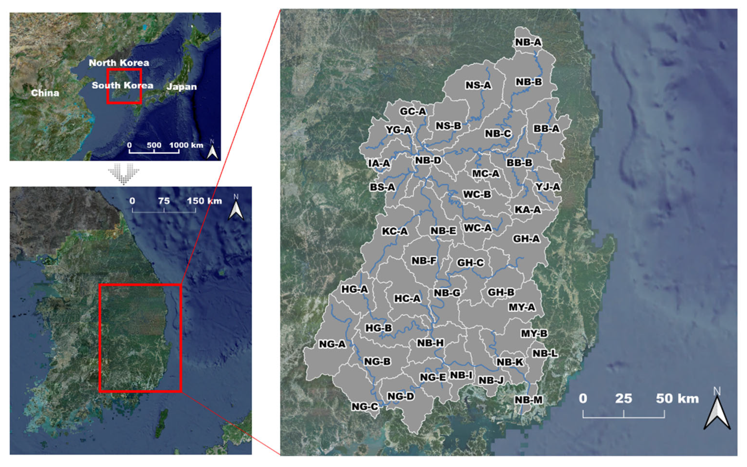
2. Materials and Methods

2.1. Data

The Nakdong River is 506.17 km long and has a watershed area of 23,384.21 km², making it the longest river in Korea, accounting for about 24 % of the country. There are about 780 rivers and seven large multi-purpose dams in the basins located in the southeast of the Korean peninsula (127° E to 129° E and 35° N to 37° N). The Nakdong river basin is divided into four major geological categories: upstream (all or part of 16 cities and counties including Taebaek and Gumi), midstream (all or part of 20 cities and counties including Daegu and Gyeongsan), west downstream (all or part of 13 cities and counties including Jinju), and east downstream (All or part of 16 cities and counties including Busan and Miryang). About 6.7 million people also live in the Nakdong river basin. Therefore, each category includes urban, agricultural, and industrial areas [34].

All data were prepared based on the 40 unit watersheds of the Nakdong River watershed based on the total maximum daily load (TMLD). The Nakdong River water quality data used as dependent variables are biological oxygen demand (BOD), total suspended matter (SS), total nitrogen (TN), and total organic carbon (TOC). The period for all river water quality concentration data is from 2015 to 2019. In this study, the time-averaged water quality concentration in each unit watershed was used since it focused on the spatial characteristics affecting river water quality. The water quality concentration data of the river was obtained from the Korean Ministry of Environment’s water environment information system [47]. Figure 1 shows the location of unit watersheds in the Nakdong river basin.

The predictors, which are independent variables, are largely divided into four families: watershed characteristics, climate, land use, and soil. In the family of watershed characteristics, predictors consist of water temperature (°C), water pH, flow rate (m³/s), watershed area (km²), watershed altitude (m), watershed slope (%), and river length (km). Water temperature, water pH, and flow rate were obtained from the Korean Ministry of Environment’s water environment information system. Since these are time-changing data, the time-averaged values were used in each unit basin. Watershed area was obtained from the Korean Ministry of Environment’s water quality TMDL information service [48], and watershed slope was obtained from the Korean Ministry of Environment’s national spatial information portal [49].

In the climate family, predictors consist of potential evapotranspiration (mm/d), (annual) precipitation (mm/d), spring precipitation (mm/d), summer precipitation (mm/d), fall precipitation (mm/d), winter precipitation (mm/d), average temperature (K), winter average temperature (K), summer average temperature (K), January lowest temperature (K), and August highest temperature (K). Predictors from the climate family were obtained from the Korean Meteorological Administration’s weather data open portal [50]. Potential evapotranspiration was calculated from weather observations using the Penman–Monteith method [51]. All data in the climate family were time averaged.

The land use family was subdivided into 23 predictors: residential area (%), industrial area (%), commercial area (%), amusement facility area (%), transportation facility area (%), public facility area (%), paddy field (%), field (%), plastic vinyl house (%), orchard (%), other cultivation (%), deciduous forests (%), coniferous forests (%), mixed forests (%), natural grassland (%), golf course (%), other grassland (%), inland wetland (%), coastal wetland (%), mining area (%), bare land (%), inland water (%), and ocean water (%). Data from the land use family were obtained from the environmental spatial information service of the Korean Ministry of Environment [52].

In the family of soil, predictors consist of soil pH, soil organic matter (g/kg), soil available phosphate acid (g/kg), soil potassium (cmol⁺/kg), soil calcium (cmol⁺/kg), soil magnesium (cmol⁺/kg), soil electrical conductivity, and soil available silicic acid (g/kg). All of these data were obtained from the Korean Agricultural Research Institute’s soil environmental information system [53].

The total number of predictors for BOD and TN is 50, and the total number of predictors for SS and TOC is 49 (excluding pollutant load). The predictors, except for the family of watershed characteristics, were converted from the data values of each station to the spatial average value of each unit watershed using the Thiessen area-weighted average method. In this work, the spatial scope of the unit watershed includes all the unit watersheds located upstream of the unit watershed, as well as the unit watershed itself. For example, we defined the spatial domain of unit watershed NG-C as containing both NG-A, NG-B, and NG-C. Thus, the spatial area of NB-M, the unit watershed located at the Nakdong river basin exit, becomes the entire Nakdong river basin.

2.2. Method

2.2.1. Identification of Predictors

Statistical models for the spatial variability of mean concentrations were assumed to be structured of linear additive models, and predictors were chosen using the exhaustive search (ES) approach [54]. Since the probability distribution of water quality concentration data and candidate predictor data is not a normal distribution, both of them have been converted to normal distributions as much as possible using Box-Cox transformations. Furthermore, the transformed data were standardized so that the mean was zero and the variance was one. ES was performed twice as follows.

It is worth mentioning that our linear additive model combined with ES is linear in terms of the structure of the equation. It is not a linear representation of the physical processes that represent hydrology and water quality at the watershed scale. A transformation process was performed to normalize the distribution of various watershed features. Water quality variables were also normalized and transformed to follow a normal distribution. A linear model linking the transformed watershed characteristics with the transformed water quality variables was constructed. Therefore, the proposed model is not a linear representation of the physical processes representing hydrology and water quality.

In the first ES, we fully explored all theoretically possible mean concentration prediction models with up to five predictors. ES is an algorithm that investigates all possible cases. That is, ES is performed by specifying the maximum number of predictors to be included out of the total number of predictors. Assuming that there are 49 candidate predictors, 49 models are fully explored if the maximum number of predictors is one, 1176 models if two, 18,424 models if three, 211,876 if four, and 1,906,884 models if five. A total of 2,138,409 models were investigated in the first ES. For each model, the corrected Akaike information criterion ($AICc$, see Equation (1)) proposed by Hurwich and Tsai [55] and model weights (see Equation (2) proposed by Burnham and Anderson [56] were calculated.

$$AI{C}_c=AIC+\frac{2K\left(K+1\right)}{nobs-K-1}$$

(1)

$$W_i=\frac{e^{-0.5{\Delta }_i}}{{{\displaystyle \sum }}_{i=1}^M{e}^{-0.5{\Delta }_i}}$$

(2)

In Equation (1), $K$ is the dimension of the model (i.e., the number of parameters), $nobs$ is the number of observations, and $M$ is the number of applied models. The $AICc$ in Equation (1) was applied to penalize overfitting models. In Equation (2), $W_i$ represents the model weight for model $i$, and ${\Delta }_i$ represents the difference between model $i$’s $AICc$ and the smallest $AICc$ among all models. Model weights are used to calculate the proportion of evidence for each predictor. In other words, the proportion of evidence for any particular predictor is calculated as the sum of the weights of the model containing that predictor [54,56].

After calculating the sum of the evidence weights for each predictor, predictors whose sum of evidence weights was not included in the top 50% were considered to be unimportant variables. These predictors were excluded from the list of candidate predictors for the second ES. A total of 24 predictors were adopted for the second ES.

In the second ES, we set the maximum number of predictors that can be included in the model at up to 10 because the number of potential predictors was halved, resulting in a reduced computational requirement. In other words, 4,540,385 models were fully explored in the second ES. Each model was evaluated using consistent AIC ($CAIC$), shown in Equation (3), which was proposed by Bozdogan (1987) [57]. The $CAIC$ in Equation (3) gives greater penalty points for overfitting models than $AICc$. In Equation (3), $nllh$ is a negative log-likelihood function.

$$CAIC=2nllh+K\left[\ln \left(nobs\right)+1\right]$$

(3)

The minimum of the $CAIC$s for all models is defined as $CAI{C}_{min}$, and the $\Delta CAIC$ for each model is calculated as in Equation (4):

$$\Delta CAIC=CAIC-CAI{C}_{min}$$

(4)

From the second ES, 20 models with the smallest $\Delta CAIC$ were selected for the preset maximum number of predictors. In other words, a total of 200 models were selected.

2.2.2. Estimation of Regression Coefficients for Statistical Models

Regression coefficients for models selected from two ES runs were estimated using Bayesian inference. The structure of the model is expressed in Equations (5) and (6):

$$y_i~N\left({\mu }_i,\sigma \right)$$

(5)

$${\mu }_i=c_0+c_1{x}_{1i}+c_2{x}_{2i}+\dots +c_k{x}_{ni}$$

(6)

The average concentration $y_i$ of a particular water quality item in the unit watershed $i$ is derived from a normal distribution with a mean ${\mu }_i$ and a standard deviation $\sigma$. The mean ${\mu }_i$ is simulated as a function of the global intercept $c_0$ and the coefficient $c_k$ of the $n$-th predictor multiplied by the value $x_n$ of the corresponding predictor. In Equation (6), $n$ is the maximum number of predictors in the model. Since the standardized predictors were applied, the prior distribution of the global intercept $c_0$ and the regression coefficient $c_k$ were assumed to be normal (i.e., the mean is 0, the standard deviation is 1). Furthermore, the prior distribution of the standard deviation $\sigma$ is assumed to be a uniform distribution between 0 and 10. Note that the prior distribution of the standard deviation $\sigma$ was set by Lintern et al. [16] as a uniform distribution between 0 and 10.

Estimation of the regression coefficients of the statistical models was carried out using the Metropolis–Hastings algorithm [58,59], which has also been used in Choi et al. [60] and Kim et al. [61]. After 4000 sampling for initial burn-in purposes, 16,000 Markov chain Monte Carlo sampling was carried out.

The accuracy of the model was evaluated using the Kling–Gupta efficiency ($KGE$) measure proposed in Gupta et al. [62]. After the model prediction values were back standardized and Box-Cox back transformed, $KGE$ was calculated by comparing them with actual observed values (i.e., those which were not Box-Cox transformed and standardized transformed). The $KGE$ is defined as follows:

$$KGE=1-\sqrt[ ]{{\left(r-1\right)}^2+{(\frac{{\sigma }_s}{{\sigma }_o}-1)}^2+{\left(\frac{{\mu }_s}{{\mu }_o}-1\right)}^2}$$

(7)

where $r$ is the correlation coefficient between the model and the observed value, ${\sigma }_s$ is the standard deviation of the model’s predicted value, ${\sigma }_o$ is the standard deviation of the observed value, ${\mu }_s$ is the average of the model’s predicted value, and ${\mu }_o$ is the average of the observed value.

Meanwhile, uncertainty in model predictions, along with model accuracy, becomes an important factor in evaluating the model’s performance since the model has been fitted from limited data [60,63,64]. The uncertainty of the model was quantified by the width of the 95% confidence interval of the water quality concentration ensemble predicted from the Metropolis–Hastings algorithm. The average width of the 95% confidence interval of the predicted water quality concentration in each unit watershed was defined as an r-factor which is a measure of uncertainty in a particular model. In other words, we conclude that the larger the $KGE$ (i.e., the higher the accuracy), and the smaller the r-factor (i.e., the smaller the uncertainty), the better the performance of the model.

3. Results

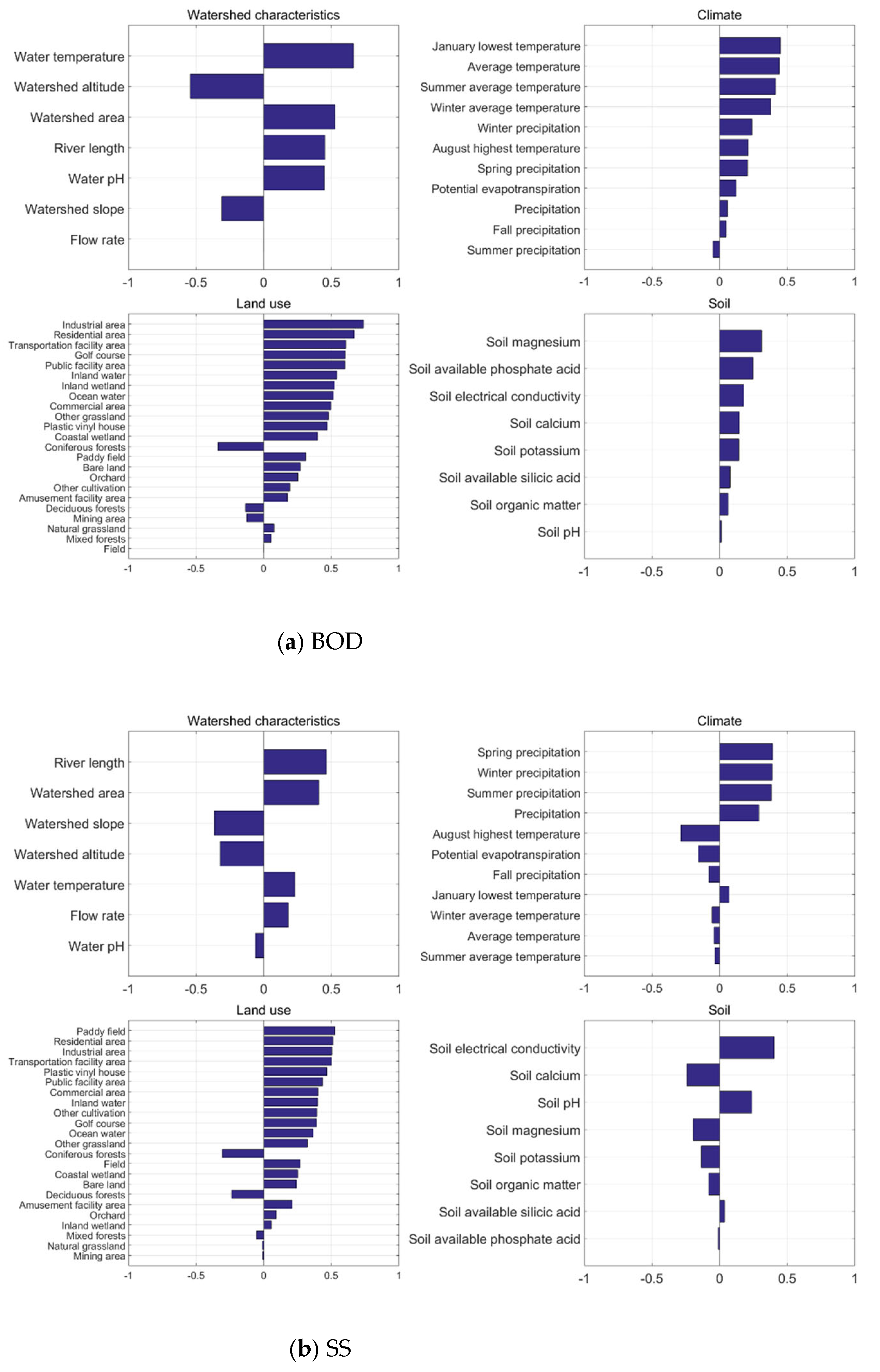
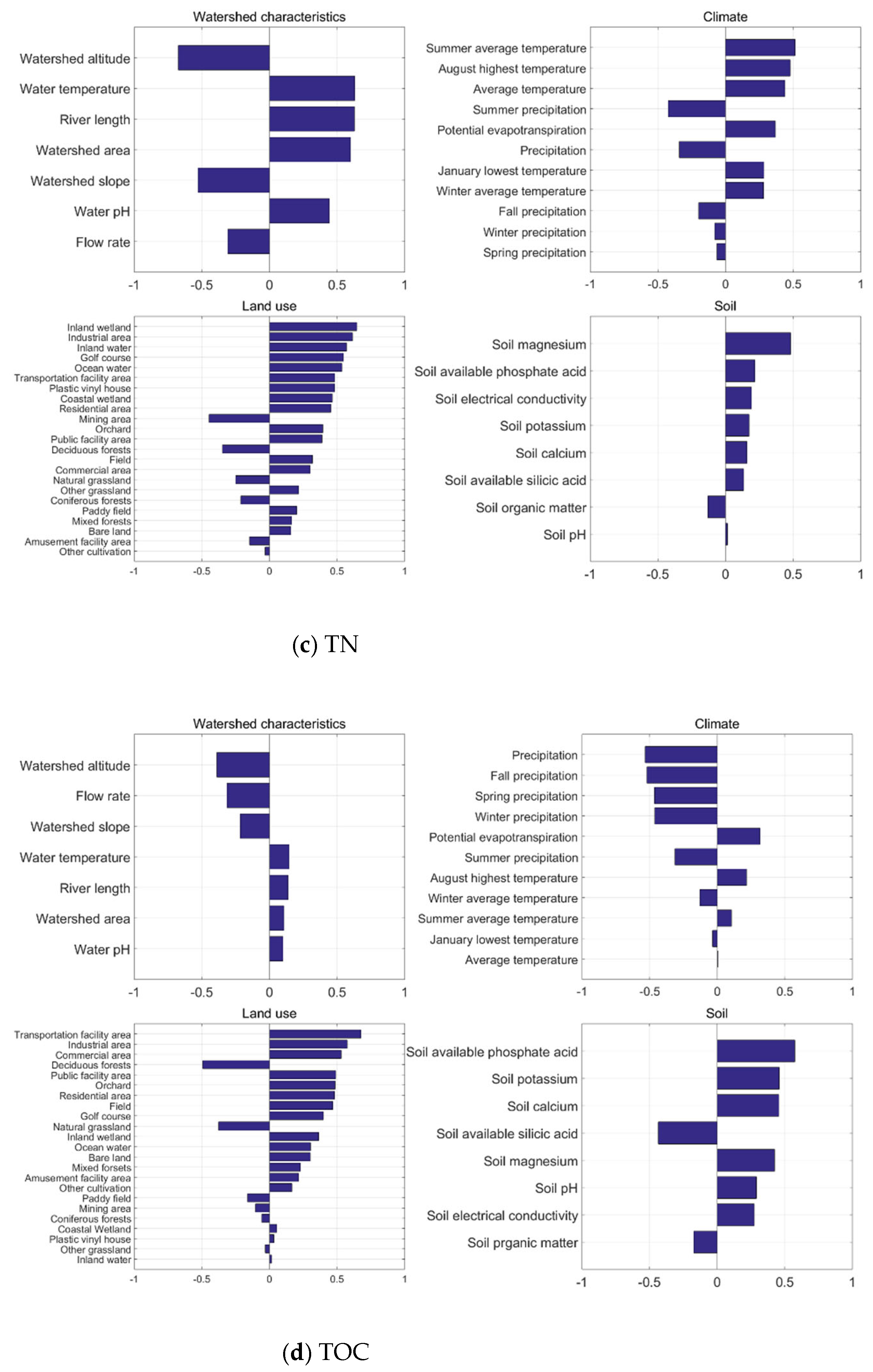
3.1. Correlation between River Water Quality and Predictors

Prior to the main analysis, correlation analyses between the Nakdong River water quality concentration and predictor variables were performed. Figure 2 shows the correlation coefficients between the water quality concentration and predictor variables.

BOD showed high correlations with water temperature, watershed area, watershed altitude, residential area, industrial area, transportation facility area, public facility area, golf course, inland wetland, inland water, and ocean water (more than 0.5 or less than –0.5). In particular, the correlation coefficient with the industrial area was the highest at 0.74. The correlation coefficients of SS was low overall, with the largest value being 0.53. Residential area, industrial area, transportation facility area, and paddy field showed high correlations, while watershed area, river length, public facility area, plastic vinyl house, and soil electrical conductivity also showed relatively high correlations (more than 0.4 or less than –0.4). The correlation coefficients of TN showed high correlations with precipitation, fall precipitation, industrial area, commercial area, transportation facility area, and soil available phosphate acid, while transportation facility area was the highest at 0.68. The correlation coefficients of TOC showed high correlations with water temperature, watershed area, watershed altitude, watershed slope, river length, summer average temperature, industrial area, golf course, inland wetland, inland water, and ocean water. It showed a high negative correlation of –0.67.

It should be noted that there is also a cross-correlation between the predictors. In general, cross-correlation was high among predictors in the same family. In other words, it can be seen that there is a possibility that the problem of multicollinearity between the predictors that constitute the regression model may occur. If predictors with multicollinearity are included in the list of significant variables, it means they are significant by themselves, so we left them as they are and proceeded with the subsequent process. In fact, unless the relationship between the finally adopted predictors is severely multicollinear (for example, the cross-correlation coefficient is 0.9 or more), it is not considered to be a problem.

3.2. Results of Exhaustive Search

Figure 3 shows the proportion of evidence derived for each predictor as a result of the first ES in ascending order. Based on this, the top 50% predictors with a high proportion of evidence were adopted as predictors for the second ES.

A total of 24 predictors were adopted in the primary ES for BOD: water temperature, water pH, watershed area, watershed altitude, river length, winter precipitation, average temperature, summer average temperature, January lowest temperature, residential area, industrial area, commercial area, transportation facility area, public facility area, other cultivation, deciduous forests, golf course, inland wetland, inland water, ocean water, soil available phosphate acid, soil calcium, soil magnesium, and soil available silicic acid. Among them, the proportion of evidence for industrial area was the highest with 0.41, and the proportion of evidence for water temperature with 0.26 was the second highest. Compared with Figure 2, the industrial area had the highest correlation coefficient with BOD among the predictors, and the industrial area also had the highest proportion of evidence. Furthermore, all predictors with high correlation coefficients in Figure 2 were adopted as predictors with a high proportion of evidence.

A total of 24 predictors were adopted in the primary ES for SS: watershed area, watershed altitude, watershed slope, river length, precipitation, spring precipitation, summer precipitation, fall precipitation, winter precipitation, average temperature, winter average temperature, summer average temperature, August highest temperature, residential area, industrial area, transportation facility area, public facility area, paddy field, field, plastic vinyl house, orchard, deciduous forests, natural grassland, and inland water. Among them, the proportion of evidence for summer precipitation was the highest with 0.22, and the proportion of evidence for paddy field was the second highest with 0.21. Compared with Figure 2, paddy field, which had the highest correlation coefficient with SS, recorded the second highest proportion of evidence. Among the predictors that had a relatively high correlation coefficient, all predictors except for soil electrical conductivity were adopted as predictors with a high proportion of evidence.

A total of 24 predictors were adopted in the primary ES for TN: watershed altitude, precipitation, spring precipitation, summer precipitation, fall precipitation, winter precipitation, winter average temperature, residential area, industrial area, commercial area, transportation facility area, public facility area, paddy field, field, orchard, deciduous forests, natural grassland, other grassland, coastal wetland, soil pH, soil available phosphate acid, soil potassium, soil magnesium, and soil available silicic acid. Among them, the proportion of evidence for the transportation facility area was the highest at 0.38, and the proportion of evidence for the precipitation, public facility area, and soil available phosphate acid was 0.2 or more. Compared with Figure 2, the transportation facility area had the highest correlation coefficient with TN, and the transportation facility area showed the highest proportion of evidence. Furthermore, all predictors with high correlation coefficients were adopted as predictors with a high proportion of evidence.

A total of 24 predictors were adopted in the primary ES for TOC: water temperature, water pH, watershed area, watershed altitude, watershed slope, river length, precipitation, summer precipitation, average temperature, summer average temperature, August highest temperature, residential area, industrial area, amusement facility area, transportation facility area, public facility area, other cultivation, inland wetland, coastal wetland, mining area, inland water, soil available phosphate acid, soil calcium, and soil magnesium. Compared with Figure 2, watershed altitude, which had the highest correlation coefficient with TOC, showed the second largest proportion of evidence. Furthermore, among the predictors with a high correlation coefficient, all predictors except golf course and ocean water were adopted as predictors with a high proportion of evidence.

Secondary ES was performed using the predictors adopted from the primary ES, and as a result, 20 models with the smallest ΔCAIC were adopted for each water quality item and the maximum number of applied predictors. That is, a total of 200 statistical models were adopted for each water quality category. When the regression coefficient of the predictor included in the adopted model and the correlation coefficient between the predictor variable and the water quality item were compared, it was confirmed that there were predictors with different signs of the regression coefficient and the correlation coefficient. Predictors with different signs from the regression coefficient and correlation coefficient are not suitable for examining the effect of spatial variability on water quality. As a result, the optimal statistical models were selected by examining the accuracy and uncertainty of the remaining models except for the models including the predictors with different signs of the regression coefficient and the correlation coefficient among the selected models.

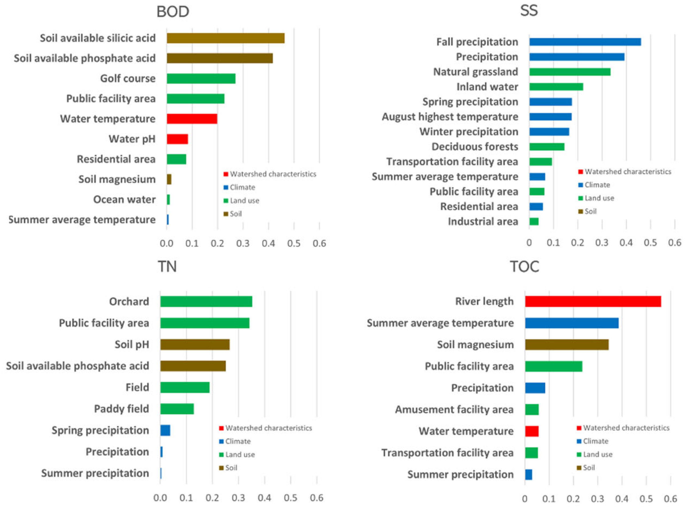
3.3. Identification of Predictors

To take into account both the accuracy and uncertainty of the model, we selected the five models with the smallest r-factor among the models with a KGE score in the top 10 percent as optimal statistical models.

Table 1. Optimal statistical models.

	Model	KGE	r-Factor	No. of Predictors
BOD	model 1	0.8642	0.4891	5
	model 2	0.8628	0.4963	6
	model 3	0.8741	0.5176	6
	model 4	0.8638	0.5238	6
	model 5	0.8625	0.5271	6
SS	model 1	0.7819	2.8677	6
	model 2	0.7862	2.9061	6
	model 3	0.7746	2.9476	6
	model 4	0.7722	2.9586	6
	model 5	0.7735	2.9665	6
TN	model 1	0.9159	0.4321	6
	model 2	0.9185	0.4450	6
	model 3	0.9169	0.4646	7
	model 4	0.9143	0.4657	7
	model 5	0.9185	0.4681	7
TOC	model 1	0.8992	0.5497	4
	model 2	0.8993	0.5512	4
	model 3	0.9294	0.5671	5
	model 4	0.9122	0.5679	5
	model 5	0.8992	0.5765	6

shows the accuracy and uncertainty of the five optimal statistical models adopted for each water quality item, and the number of predictors contained in the model. The accuracy and uncertainty of optimal statistical models in each unit watershed are shown in Figures S1–S4 in the Supplementary Materials.

The optimal statistical models consist of three to seven predictors. For BOD, TN, and TOC, the KGE of all the statistical models is 0.8 or higher, while the statistical models all exhibit relatively low levels of uncertainty at 0.6 or lower. For SS, all statistical models had the lowest accuracy among the water quality variables with a KGE of less than 0.8 for each model, while the uncertainty of the statistical models was the highest among the water quality variables.

Predictors forming an optimal statistical model allow us to see what factors have a major impact on the spatial variability of river water quality. Figure 4 represents the predictors included in the optimal statistical models and their corresponding regression coefficients. Figure 4 expresses the absolute value of the regression coefficient as the length of the bar to facilitate the relative comparison between the predictors.

In the statistical models for BOD, a total of nine predictors were selected as environmental factors affecting the BOD concentration in streams: water temperature, water pH in the family of watershed characteristics; summer average temperature in the climate family; residential area, public facility area, golf course, and ocean water in the land use family; and soil available phosphate acid, soil magnesium, and soil available silicic acid from the soil family. Among them, water temperature and public facility area were included in four models, while golf course, soil available phosphate acid, and soil available silicic acid were included in all models. In particular, the regression coefficient values in all models were above 0.4 for both soil available phosphate acid and soil available silicic acid.

In the statistical models for SS, a total of 13 predictors were adopted as environmental factors affecting SS concentration in rivers: precipitation, spring precipitation, fall precipitation, winter precipitation, summer average temperature, and August highest temperature in the climate family; and residential area, industrial area, transportation facility area, public facility area, deciduous forests, natural grassland, and inland water in the land use family. Among these, fall precipitation, natural grassland, and inland water were included in all models.

In the statistical models for TN, a total of nine predictors were selected as environmental factors affecting TN concentration in rivers: precipitation, spring precipitation, and summer precipitation in the climate family; public facility area, paddy field, field, and orchard in the land use family; and soil pH and soil available phosphate acid from the soil family. Among them, public facility area, field, orchard, soil available phosphate acid, and soil pH were included in all models, while the regression coefficient values of all predictors except field were relatively high.

In statistical models for TOC, a total of nine predictors were selected as environmental factors affecting TOC concentrations in streams: water temperature and river length in the family of watershed characteristics; precipitation, summer precipitation, and summer average temperature in the climate family; amusement facility area, transportation facility area, and public facility area in the land use family; and soil magnesium in the soil family. Of these, river length and soil magnesium were included in all models.

4. Discussion

4.1. Influences of Predictors

The importance of predictive variables can be investigated from two perspectives. How many models contain a specific predictor is an important indicator of the importance of the predictor. If many models include this predictor, it means that the predictor has a great influence on the spatial variability of water quality. The second point to mention is the influence (i.e., the value of the regression coefficient) that the predictor included in the model had within the model. Even if the predictor is included in a certain model, if the absolute value of the regression coefficient for the predictor is very small, it is difficult to interpret great meaning. Since the number of models including a certain predictor and the influence of the predictor in the model including the predictor vary, it is necessary to investigate these characteristics in more detail.

We tried to find predictors that have a relatively greater impact on river water quality by quantifying the influence of predictors in the model. In a model containing a predictor, the absolute value of its regression coefficient was divided by the number of predictors that constitute the model, and then the influence of the predictor was quantified by summing it up for all models containing the predictor. Figure 5 is the result of a list of predictors in order of high influence.

Models for BOD were influential, in order of most to least, for soil available silicic acid, soil available phosphate acid, golf course, public facility area, and water temperature. The influence of the soil available silicic acid was 0.46, and the influence of the soil available phosphate acid was 0.42. That is, it can be recognized that the predictors of the soil family and the land use family have a significant impact on BOD.

In the models for SS, the influence was highest starting with fall precipitation, precipitation, natural grassland, inland water, spring precipitation, and finally August highest temperature. The influence of fall precipitation was 0.46, and the influence of precipitation and natural grassland was more than 0.3. It can be recognized that the predictor variables in the climate family and the land use family have a large influence on SS.

In the models for TN, orchard, public facility area, soil pH, soil available phosphate acid, and field were highly influential predictors. The influence of orchard, public facility area, and soil available phosphate acid was greater than 0.3. It can be recognized that predictors in the land use family and the soil family have a significant impact on TN.

In the models for TOC, the influence was highest starting with river length, summer average temperature, soil magnesium, public facility area, and finally precipitation. The influence of river length was 0.56, while the influence of summer average temperature and soil magnesium was more than 0.3. It can be recognized that the predictors in the climate, land use, and soil families, as well as the family of watershed characteristics, have various influences on TOC concentrations in the river.

4.2. Identification of Key Predictors

In order to adopt the main predictors that have a relatively large impact among the selected predictors that affect river water quality concentrations, uncertainty of the predictors along with their influence should also be considered. To compare the uncertainties of various predictors with each other, a coefficient of variation was calculated from the posterior distribution of the regression coefficients corresponding to each predictor. Figure 6 shows the coefficient of variation in the predictors. Overall, we found that regression coefficients corresponding to highly influential predictors were less uncertain.

To find environmental factors that have a relatively greater impact on water quality data among the adopted predictors, the top five predictors were re-adopted in the order of high influence from Figure 5. We also re-adopted five predictors with low uncertainty from the results of Figure 6. Among them, overlapping predictors were finally identified as key predictors.

Key predictors affecting BOD were water temperature in the watershed characteristics family, and soil available phosphate acid and soil available silicic acid in the soil family. Key predictors affecting SS have all been identified in the climate family: precipitation, spring precipitation, and fall precipitation. Key predictors affecting TN were public facility area, orchard, and field in the land use family, and soil pH and soil available phosphate acid in the soil family. Key predictors affecting TOC were river length in the watershed characteristics family, summer average temperature in the climate family, public facility area in the land use family, and soil magnesium in the soil family.

The fact that all the key predictors that affect SS are in the climate family suggests that managing SS in the Nakdong river basin is very difficult. This is because it is difficult for us to artificially control climatological factors. The dependence of SS on climatological factors means that SS may respond most directly to the effects of upcoming or already approaching climate change. The list of key predictors affecting BOD, TN, and TOC are all included in the land use family. Among the predictors of the land use family, the fact that predictors representing urban land use (e.g., residential area and public facility area) were identified as key predictors shows that the river water quality in the Nakdong river basin is greatly influenced by anthropogenic factors. This means that the population represented by residential area or public facility area is still an important predictor of river water quality. Considering that the Nakdong river basin is almost completely equipped with water pollution prevention facilities for point pollution sources that meet the water quality regulation standards, the results of this study suggest that, rather than focusing on the expansion of point source treatment facilities, additional water quality management measures for non-point pollutant sources can help improve the water quality of the Nakdong River. In addition, land use patterns will be more affected in the future due to continued urbanization and population movement. From this point of view, stormwater management based on the concept of low-impact development will also need to be highlighted as a more important factor in the water quality management of the Nakdong River. Another thing to mention is soil available phosphate acid, a key predictor of the soil family. The fact that the soil available phosphate acid has a significant impact on river water quality levels is directly linked to fertilizer injection in agricultural land. In summary, from the fact that urban land use fractions and fertilizer usage have been identified as key predictors affecting river water quality, how to control the effects of pollutant sources by human activities is the most important issue in water quality management in the Nakdong river basin.

We performed data-based modeling based on uncertainty to identify general impacts on water quality from many of the applicable potential pollutants, including natural and anthropogenic sources. However, in order to accurately identify various factors influencing river water quality, it will always be necessary to develop a model based on a more advanced approach, and to expand more diverse observational data, including pollutant source and water quality concentration data.

5. Conclusions

In this study, we selected environmental factors that affect the water quality concentration of rivers by combining the river water quality concentration data observed in 40 unit watersheds of the Nakdong river basin during the period from 2015 to 2019, with 50 environmental factors obtained in each unit watershed. To construct a statistical model in a linear additive model form, a two-step exhaustive search approach and a process for estimating regression coefficients using Bayesian inference were executed. Through a series of processes to find optimal statistical models that take into account both the accuracy and uncertainty of statistical models, we identified key factors that most affect river water quality in the Nakdong river basin.

Residential area, soil available phosphate acid, and soil available silicic acid have been identified as key predictors that affect BOD. BOD could be recognized to be greatly affected by the soil properties of the basin. The river SS concentration in the Nakdong river basin is more dependent on precipitation than on ground characteristics, such as terrain, soil, and land use patterns. Public facility area, orchard, soil available phosphate acid, and others have been identified as key predictors affecting TN. In other words, it was recognized that land use patterns and soil characteristics in the basin had a significant impact on river TN concentrations. TOC was related to a variety of environmental factors. The key predictors affecting TOC were river length and summer average temperature.

The length of the main stream of the Nakdong River is more than 500 km. There is a large industrial complex in the upper reaches of the Nakdong River, and a large city with a population of 2.5 million in the middle of the Nakdong River. At the mouth of the Nakdong River, there is another metropolis with a population of 3.5 million. The water intake for drinking water for residents of the large city in the middle of the Nakdong River is the raw water of the main Nakdong River, including industrial wastewater discharged from the upstream. In addition, the water intake for drinking water for residents of the large city at the mouth of the Nakdong River is raw water from the main Nakdong River, including industrial wastewater from the upstream and domestic sewage from the middle stream. Due to such urban location conditions, the Nakdong river basin has been subjected to thorough water quality management for point pollution sources. However, the results of this study reveal that the water quality of the Nakdong River is greatly affected by soil characteristics and land use characteristics. The fact that soil properties such as soil available phosphate acid, soil available silicic acid, and soil magnesium were selected as major predictors means that agricultural management, especially livestock management, is very important to improve the water quality of the Nakdong River. In addition, the fact that urban land-use characteristics, such as public facility area, were identified as the main influencing factors on the spatial average water quality of major streams in the Nakdong river basin shows that intensive management of non-point pollutants is essential for improving the water quality of the Nakdong river basin. In addition, continuous urbanization and increased demand for livestock products are expected to have a greater impact on water quality in the future. From this point of view, the paradigm for water quality management in the Nakdong river basin needs to be changed from a point source-centered management to agricultural pollution source management and urban non-point pollution source management.

The model developed in this study can be applied to investigate the river water quality of the Nakdong river basin for various climate change and land use scenarios in the future. In addition, if the results of this study are applied to the driver-pressure-state-impact-response (DPSIR) framework to analyze the causal relationship of river water quality deterioration in the future, it can help analyze water quality problems within the Nakdong river basin community and create an appropriate community-based management model. Furthermore, it could be used to provide appropriate policy recommendations. Finally, based on the model for the spatial variability of the average water quality response developed in this study, it is expected to serve as a cornerstone for advancing the model for the temporal variability of water quality.

References

1. Loucks, D.P.; van Beek, E.; Stedinger, J.R.; Dijkman, J.P.M.; Villars, M.T. Water Resources Systems Planning and Management: An Introduction to Methods, Models and Applications; UNESCO: Paris, France, 2005. [Google Scholar]
2. Schwarzenbach, R.P.; Egli, T.; Hofstetter, T.B.; Von Gunten, U.; Wehrli, B. Global water pollution and human health. Annu. Rev. Environ. Resour. 2010, 35, 109–136. [Google Scholar] [CrossRef]
3. UN-Water Statement on Water Quality. Available online: www.unwater.org. (accessed on 22 February 2021).
4. Simeonov, V.; Stratis, J.A.; Samara, C.; Zachariadix, G.; Voutsa, D.; Anthemidis, A.; Sofoniou, M.; Kouimtzis, T.H. Assessment of the surface water quality in Northern Greece. Water Res. 2003, 37, 4119–4124. [Google Scholar] [CrossRef]
5. Sánchez, E.; Colmenarejo, M.F.; Vincente, J.; Rubio, A.; Garcia, M.; Travieso, L.; Borja, R. Use of the water quality index and dissolved oxygen deficit as simple indicators of watersheds pollution. Ecol. Indic. 2007, 7, 315–328. [Google Scholar] [CrossRef]
6. Hunter, P.R. Climate change and waterborne and vector-borne disease. J. Appl. Microbiol. 2003, 94, 37–46. [Google Scholar] [CrossRef]
7. Paul, M.J.; Meyer, J.L. Streams in the urban landscape. Annu. Rev. Ecol. Syst. 2001, 32, 333–365. [Google Scholar] [CrossRef]
8. Meybeck, M.; Chapman, D.; Helman, P. Global Freshwater Quality: A First Assessment. In Global Environment Monitoring System; Basil Blackwell: Cambridge, UK, 1990. [Google Scholar]
9. Cuo, L.; Yongxin, Z.; Yanhong, G.; Zhenchun, H.; Luosang, C. The impacts of climate change and land cover/use transition on the hydrology in the upper Yellow River Basin, China. J. Hydrol. 2013, 502, 37–52. [Google Scholar] [CrossRef]
10. Murray-Hudson, M.; Wolski, P.; Ringrose, S. Scenarios of the impact of local and upstream changes in climate and water use on hydro-ecology in the Okavango Delta, Botswana. J. Hydrol. 2006, 331, 73–84. [Google Scholar] [CrossRef]
11. Novotny, E.V.; Stefan, H.G. Stream flow in Minnesota: Indicator of climate change. J. Hydrol. 2007, 334, 319–333. [Google Scholar] [CrossRef]
12. Heathwaite, A.L. Multiple stressors on water availability at global to catchment scales: Understanding human impact on nutrient cycles to protect water quality and water availability in the long term. Freshw. Biol. 2010, 55, 241–257. [Google Scholar] [CrossRef]
13. Kim, J.; Choi, J.; Choi, C.; Park, S. Impacts of changes in climate and land use/land cover under IPCC RCP scenarios on streamflow in the Hoeya River Basin, Korea. Sci. Total Environ. 2013, 452, 181–195. [Google Scholar] [CrossRef]
14. Mandal, P.; Upadhyay, R.; Hasan, A. Seasonal and spatial variation of Yamuna River water quality in Delhi, India. Environ. Monit. Assess. 2010, 170, 661–670. [Google Scholar] [CrossRef]
15. Wang, Q.; Wu, X.; Zhao, B.; Qin, J.; Peng, T. Combined multivariate statistical techniques, water pollution index (WPI) and Daniel trend test methods to evaluate temporal and spatial variations and trends of water quality at Shanchong River in the Northwest Basin of Lake Fuxian, China. PLoS ONE 2015, 10, e0118590. [Google Scholar] [CrossRef] [Green Version]
16. Lintern, A.; Webb, J.A.; Ryu, D.; Liu, S.; Waters, D.; Leahy, P.; Bende-Michl, U.; Western, A.W. What are the key catchment characteristics affecting spatial differences in riverine water quality? Water Resour. Res. 2018, 54, 7252–7272. [Google Scholar] [CrossRef]
17. Allan, J.D. Influence of land use and landscape setting on the ecological status of rivers. Limnetica 2004, 23, 187–197. [Google Scholar]
18. Suarez, J.; Puertas, J. Determination of COD, BOD, and suspended solids loads during combined sewer overflow (CSO) events in some combined catchments in Spain. Ecol. Eng. 2005, 24, 199–217. [Google Scholar] [CrossRef]
19. Drewry, J.J.; Newham, L.T.H.; Greene, R.S.B.; Jakeman, A.J.; Croke, B.F.W. A review of nitrogen and phosphorus export to waterways: Context for catchment modelling. Mar. Freshw. Res. 2006, 57, 757–774. [Google Scholar] [CrossRef]
20. Giri, S.; Qiu, Z. Understanding the relationship of land uses and water quality in twenty first century: A review. J. Environ. Manag. 2016, 173, 41–48. [Google Scholar] [CrossRef] [Green Version]
21. Vieira, J.; Fonseca, A.; Vilar, V.J.; Boaventura, R.A.; Botelho, C.M. Water quality modelling of Lis river, Portugal. Environ. Sci. Pollut. Res. 2013, 20, 508–524. [Google Scholar] [CrossRef] [PubMed]
22. Venkatramanan, S.; Chung, S.Y.; Lee, S.Y.; Park, N. Assessment of river water quality via environmentric multivariate statistical tools and water quality index: A case study of Nakdong River Basin, Korea. Carpathian J. Earth Environ. Sci. 2014, 9, 125–132. [Google Scholar]
23. Sun, W.; Xia, C.; Xu, M.; Guo, J.; Sun, G. Application of modified water quality indices as indicators to assess the spatial and temporal trends of water quality in the Dongjiang River. Ecol. Indic. 2016, 66, 306–312. [Google Scholar] [CrossRef]
24. Valentukevičienė, M.; Bagdžiūnaitė-Litvinaitienė, L.; Chadyšas, V.; Litvinaitis, A. Evaluating the impacts of integrated pollution on water quality of the trans-boundary neris (viliya) river. Sustainability 2018, 10, 4239. [Google Scholar] [CrossRef] [Green Version]
25. Ducharne, A.; Baubion, C.; Beaudoin, N.; Benoît, M.; Billen, G.; Brisson, N.; Garnier, J.; Kieken, H.; Lebonvallet, S.; Ledoux, E.; et al. Long term prospective of the Seine River system: Confronting climatic and direct anthropogenic changes. Sci. Total Environ. 2007, 375, 292–311. [Google Scholar] [CrossRef]
26. Choi, D.; Jun, H.; Shin, H.S.; Yoon, Y.S.; Kim, S. The effect of climate change on Byeongseong stream’s water quantity and quality. Desalination Water Treat. 2010, 19, 105–112. [Google Scholar] [CrossRef]
27. Shrestha, S.; Bhatta, B.; Shrestha, M.; Shrestha, P.K. Integrated assessment of the climate and landuse change impact on hydrology and water quality in the Songkhram River Basin, Thailand. Sci. Total Environ. 2018, 643, 1610–1622. [Google Scholar] [CrossRef]
28. Gholami, S.; Srikantaswamy, S. Statistical multivariate analysis in the assessment of river water quality in the vicinity of KRS Dam, Karnataka, India. Nat. Resour. Res. 2009, 18, 235–247. [Google Scholar] [CrossRef]
29. Fan, X.; Cui, B.; Zhao, H.; Zhang, Z.; Zhang, H. Assessment of river water quality in Pearl River Delta using multivariate statistical techniques. Procedia Environ. Sci. 2010, 2, 1220–1234. [Google Scholar] [CrossRef] [Green Version]
30. Massoud, M.A. Assessment of water quality along a recreational section of the Damour River in Lebanon using the water quality index. Environ. Monit. Assess. 2012, 184, 4151–4160. [Google Scholar] [CrossRef] [PubMed]
31. Lin, Y.; Han, P.; Huang, Y.; Yuan, G.L.; Guo, X.; Li, J. Source identification of potentially hazardous elements and their relationships with soil properties in agricultural soil of the Pinggu district of Beijing, China: Multivariate statistical analysis and redundancy analysis. J. Geochem. Explor. 2017, 173, 110–118. [Google Scholar] [CrossRef]
32. Misaghi, F.; Delgosha, F.; Razzaghmanesh, M.; Myers, B. Introducing a water quality index for assessing water for irrigation purposes: A case study of the Ghezel Ozan River. Sci. Total Environ. 2017, 589, 107–116. [Google Scholar] [CrossRef]
33. Zamani-Ahmadmahmoodi, R.; Jafari, A.; Alibeygi-Beni, H. Potential ecological risk assessment, enrichment, geoaccumulation, and source identification of metals in the surface sediments of Choghakhor Wetland, Iran. Environ. Earth Sci. 2017, 76, 1–9. [Google Scholar] [CrossRef]
34. Han, S.; Kim, E.; Kim, S. The water quality management in the Nakdong River watershed using multivariate statistical techniques. KSCE J. Civ. Eng. 2009, 13, 97–105. [Google Scholar] [CrossRef]
35. Fathi, E.; Zamani-Ahmadmahmoodi, R.; Zare-Bidaki, R. Water quality evaluation using water quality index and multivariate methods, Beheshtabad River, Iran. Appl. Water Sci. 2018, 8, 1–6. [Google Scholar] [CrossRef] [Green Version]
36. Arnold, J.G.; Fohrer, N. SWAT2000: Current capabilities and research opportunities in applied watershed modelling. Hydrol. Process. Int. J. 2005, 19, 563–572. [Google Scholar] [CrossRef]
37. Argent, R.M.; Perraud, J.M.; Rahman, J.M.; Grayson, R.B.; Podger, G.M. A new approach to water quality modelling and environmental decision support systems. Environ. Model. Softw. 2009, 24, 809–818. [Google Scholar] [CrossRef]
38. Abbaspour, K.C.; Rouholahnejad, E.; Vaghefi, S.; Srinivasan, R.; Yang, H.; Kløve, B. A continental-scale hydrology and water quality model for Europe: Calibration and uncertainty of a high-resolution large-scale SWAT model. J. Hydrol. 2015, 524, 733–752. [Google Scholar] [CrossRef] [Green Version]
39. Luo, Y.; Zhang, M. Management-oriented sensitivity analysis for pesticide transport in watershed-scale water quality modeling using SWAT. Environ. Pollut. 2009, 157, 3370–3378. [Google Scholar] [CrossRef]
40. Boskidis, I.; Gikas, G.D.; Pisinaras, V.; Tsihrintzis, V.A. Spatial and temporal changes of water quality, and SWAT modeling of Vosvozis river basin, North Greece. J. Environ. Sci. Health Part A 2010, 45, 1421–1440. [Google Scholar] [CrossRef]
41. Poudel, D.D.; Lee, T.; Srinivasan, R.; Abbaspour, K.; Jeong, C.Y. Assessment of seasonal and spatial variation of surface water quality, identification of factors associated with water quality variability, and the modeling of critical nonpoint source pollution areas in an agricultural watershed. J. Soil Water Conserv. 2013, 68, 155–171. [Google Scholar] [CrossRef] [Green Version]
42. Kurunç, A.; Yürekli, K.; Cevik, O. Performance of two stochastic approaches for forecasting water quality and streamflow data from Yeşilιrmak River, Turkey. Environ. Model. Softw. 2005, 20, 1195–1200. [Google Scholar] [CrossRef]
43. Parmar, K.S.; Bhardwaj, R. Statistical, time series, and fractal analysis of full stretch of river Yamuna (India) for water quality management. Environ. Sci. Pollut. Res. 2015, 22, 397–414. [Google Scholar] [CrossRef]
44. Kisi, O.; Parmar, K.S. Application of least square support vector machine and multivariate adaptive regression spline models in long term prediction of river water pollution. J. Hydrol. 2016, 534, 104–112. [Google Scholar] [CrossRef]
45. Chang, H. Spatial and temporal variations of water quality in the Han River and its tributaries, Seoul, Korea, 1993–2002. Water Air Soil Pollut. 2005, 161, 267–284. [Google Scholar] [CrossRef]
46. Mei, K.; Liao, L.; Zhu, Y.; Lu, P.; Wang, Z.; Dahlgren, R.A.; Zhang, M. Evaluation of spatial-temporal variations and trends in surface water quality across a rural-suburban-urban interface. Environ. Sci. Pollut. Res. 2014, 21, 8036–8051. [Google Scholar] [CrossRef] [PubMed] [Green Version]
47. Water Environment Information System (WEIS). Available online: http://water.nier.go.kr (accessed on 1 August 2020).
48. Total Pollution Load Management System. Available online: http://tmdlms.nier.go.kr (accessed on 1 August 2020).
49. National Spatial Data Infrastructure Portal (NSDI). Available online: http://data.nsdi.go.kr (accessed on 1 August 2020).
50. Open MET Data Portal. Available online: http://data.kma.go.kr (accessed on 1 August 2020).
51. Allen, R.G.; Pereira, L.S.; Raes, D.; Smith, M. Crop Evapotranspiration-Guidelines for Computing Crop Water Requirements-FAO Irrigation and Drainage Paper 56; FAO: Rome, Italy, 1998; p. 300. [Google Scholar]
52. Environmental Geographic Information Service (EGIS). Available online: https://egis.me.go.kr (accessed on 1 August 2020).
53. Korean Soil Information System. Available online: http://soil.rda.go.kr (accessed on 1 August 2020).
54. Saft, M.; Peel, M.C.; Western, A.W.; Zhang, L. Predicting shifts in rainfall-runoff partitioning during multiyear drought: Roles of dry period and catchment characteristics. Water Resour. Res. 2016, 52, 9290–9305. [Google Scholar] [CrossRef]
55. Hurvich, C.M.; Tsai, C.L. Regression and time series model selection in small samples. Biometrika 1989, 76, 297–307. [Google Scholar] [CrossRef]
56. Burnham, K.P.; Anderson, D.R. Model Selection and Multimodel Inference: A Practical Information-Theoretic Approach, 2nd ed.; Springer: Berlin/Heidelberg, Germany, 2004. [Google Scholar]
57. Bozdogan, H. Model selection and Akaike’s information criterion (AIC): The general theory and its analytical extensions. Psychometrika 1987, 52, 345–370. [Google Scholar] [CrossRef]
58. Metropolis, N.; Rosenbluth, A.W.; Rosenbluth, M.N.; Teller, A.H.; Teller, E. Equation of state calculations by fast computing machines. J. Chem. Phys. 1953, 21, 1087–1092. [Google Scholar] [CrossRef] [Green Version]
59. Hastings, W.K. Monte Carlo sampling methods using Markov chains and their applications. J. Oxf. Acad. 1970, 57, 97–109. [Google Scholar] [CrossRef]
60. Choi, J.; Lee, O.; Won, J.; Kim, S. Stochastic Simple Hydrologic Partitioning Model Associated with Markov Chain Monte Carlo and Ensemble Kalman Filter. J. Korean Soc. Water Environ. 2020, 36, 353–363. [Google Scholar] [CrossRef]
61. Kim, R.; Won, J.; Choi, J.; Lee, O.; Kim, S. Application of Bayesian Approach to Parameter Estimation of TANK Model: Comparison of MCMC and GLUE Methods. J. Korean Soc. Water Environ. 2020, 36, 300–313. [Google Scholar] [CrossRef]
62. Gupta, H.V.; Kling, H.; Yilmaz, K.K.; Martinez, G.F. Decomposition of the mean squared error and NSE performance criteria: Implications for improving hydrological modelling. J. Hydrol. 2009, 377, 80–91. [Google Scholar] [CrossRef] [Green Version]
63. Muleta, M.K.; Nicklow, J.W. Sensitivity and uncertainty analysis coupled with automatic calibration for a distributed watershed model. J. Hydrol. 2005, 306, 127–145. [Google Scholar] [CrossRef] [Green Version]
64. Gallagher, M.; Doherty, J. Parameter estimation and uncertainty analysis for a watershed model. Environ. Model. Softw. 2007, 22, 1000–1020. [Google Scholar] [CrossRef]
Figure 1. 40 TMDL unit watersheds across the Nakdong river basin.
Sustainability 13 11319 g001
Figure 2. Cross-correlation coefficients between water quality concentration data and predictor variables: (a) BOD; (b) SS; (c) TN; (d) TOC.
Sustainability 13 11319 g002aSustainability 13 11319 g002b
Figure 3. Sum of the evidence weights of predictor variables.
Sustainability 13 11319 g003
Figure 4. Regression coefficients corresponding to predictor variables included in statistical models.
Sustainability 13 11319 g004
Figure 5. Influence of predictor variables.
Sustainability 13 11319 g005
Figure 6. Uncertainty of predictor variables through the coefficient of variation.
Sustainability 13 11319 g006