Article

Estimation of the Evapotranspiration and Crop Coefficients of Bell Pepper Using a Removable Weighing Lysimeter: A Case Study in the Southeast of Spain

by
Laura Ávila-Dávila
1,2,*,
José Miguel Molina-Martínez
2,
Carlos Bautista-Capetillo
1,*,
Manuel Soler-Méndez
2,
Cruz Octavio Robles Rovelo
1,
Hugo Enrique Júnez-Ferreira
1 and
Julián González-Trinidad
1
1
Doctorado en Ciencias de la Ingeniería, Universidad Autónoma de Zacatecas, Zacatecas 98160, Mexico
2
Research Group Ingeniería Agromótica y del Mar, Universidad Politécnica de Cartagena, 30203 Cartagena, Spain
*
Authors to whom correspondence should be addressed.
Sustainability 2021, 13(2), 747; https://doi.org/10.3390/su13020747
Submission received: 3 December 2020 / Revised: 9 January 2021 / Accepted: 10 January 2021 / Published: 14 January 2021
(This article belongs to the Special Issue Sustainable Applications in Agriculture)

Abstract

:
Water use efficiency is essential in semiarid regions of Spain, and it can be achieved through a precise knowledge of the real crop water requirements (CWR). The Food and Agriculture Organization of the United Nations (FAO) offers standardized crop coefficients to establish the CWR. However, these coefficients can change due to different conditions, such as climatic variations and cultivation practices. In this work, the evapotranspiration ( E T C l y s ) and crop coefficients ( K C l y s ) of bell pepper were obtained with a compact removable weighing lysimeter between February and August for two crop seasons (2019 and 2020). E T C l y s was determined from the water balance, and the K C l y s values were determined as the ratio of the crop evapotranspiration, measured on the removable weighing lysimeter, and the reference evapotranspiration. The K C l y s average values for the bell pepper in the initial, middle, and final stages were 0.57, 1.06, and 0.80, respectively. K C regression models were obtained as a function of the fraction thermal units, achieving a maximum correlation of 0.67 ( R 2 ). In general, the K C values obtained in this research work were lower in the initial and in the final stages and larger in the middle stage in comparison with the FAO-56 values and other research works values in semiarid conditions. The bell pepper yield increased by 7.72% in 2019 and by 3.49% in 2020 compared to the yield reported by the Ministry of the Environment and Rural and Marine Areas of the Spanish Government in 2019 and with a minimum water loss through drainage. The results in this work can help farmers to determine the crop water requirements and to improve the system efficiency in semiarid locations with similar conditions to those in the study.

1. Introduction

The irrigation areas in southeast Spain are characterized by limited water resources due to a semiarid climate. The Mediterranean basin has very hot summers that increase the crop water demand via an increase in the crop evapotranspiration rate [1,2,3]. Insufficient water for crop management causes poor water distribution and a reduction in agricultural yield, which is associated with less growth and crop development [4,5]; therefore, strategies must be adopted in order to optimize water resources and to obtain profitable crops [1].
In the Mediterranean area, Andalusia, Murcia, and Valencia are the three main regions of horticultural production, mostly involving spring–summer crops. The bell pepper production in this area mainly occurs in the Murcia region, where greenhouses reach up to 82% of the total cultivated hectares while open-field cultivation represents only 18%. The average greenhouse yield is 30% higher than the yield of open fields [6]. According to Nikolau et al. [7], the use of greenhouses allows a more efficient water use in comparison to open-field cultivation because the plastic covering reduces soil evaporation, with a 38% reduction in the water requirements of bell pepper.
In agricultural areas with limited water resources, such as the Mediterranean area, it is common to use a drip irrigation system due to its punctual application [5]; however, if the irrigation system is not properly managed, there will be water losses, usually due to run-off or water leaks in the conduction system itself.
In order to achieve the optimal irrigation application and to maximize its efficiency, it is necessary to know the precise amount of water required by the crop for its specific development conditions [4,8]. These water requirements can be estimated accurately through a water balance, which quantifies the input and output flows of the soil profile in the crop root zone [8,9,10]; in addition, a water balance helps to reduce water losses and to diagnose the irrigation method itself [11].
There are different and indirect methodologies for estimation of the crop water requirements based on the crop evapotranspiration ( E T C ), such as the standard approach proposed by the Food and Agriculture Organization of the United Nations (FAO), which uses the concept of the reference evapotranspiration ( E T O ) and crop coefficient ( K C ). This methodology has two steps. The first uses climatic variables such as the relative air humidity, the sunshine hours, the solar radiation, the wind speed, and the air temperature in order to obtain the E T O that refers to a uniformly growing crop, similar to a field of green grass, well irrigated and with a uniform height. This is called the FAO Penman–Monteith method and represents the effect of climate on water requirements [12].
The second step refers to the K c that represents the effect of the crop growth with time as a coefficient. For this coefficient, the FAO proposes two approaches in order to integrate the physical and physiological crop properties. The first approach is called single coefficient and integrates the E T O and the E T C ( K c = E T C / E T O ), while the second approach separates evaporation and transpiration. There are different ways to measure the K C . One method considers the crop stress through the fraction thermal units or growth degree days from the average air temperature. Fraction thermal units measure the accumulated heat above the base temperature, which is different between crop varieties; plant growth is zero when the temperature is below the base temperature [13,14]. Similarly, K C can be determined in the days after planting (DAP) [13] from vegetation indexes and satellite image processing [15,16], or as a percentage of green coverage via the processing of digital photos [2].
In this context, a weighing lysimeter provides a direct method to measure the E T C through the mass balance of an isolated soil volume [17]. The use of weighing lysimetry in the E T C estimation has been widely studied [3,18,19,20,21], and it has also been used to study the flows involved in the water balance and solutes in soil profiles under different conditions [22], such as dew, fog and frost [23], precipitation [24,25,26,27,28], and percolation [29]. One of the main features of such a device is the high accuracy, allowing its use to establish and calibrate different mathematical models [9,17].
Weighing lysimeters usually have large dimensions and require a large set-up area and specialized maintenance, making them expensive and of limited use for research purposes. The results from lysimetry research can be used by farmers when the conditions are similar to those in the experiment [30]. Ruiz-Peñalver et al. [30] and Nicolás-Cuevas et al. [31] developed compact and transportable weighing lysimeters that can be used in commercial plots to evaluate the irrigation application efficiencies or for estimating the crop water requirements; once the harvest is finished, the lysimeters are easy to move. Other small commercial lysimeters have been produced by the METER Group® (USA) [32] and UGT Company (Germany) [33].
The objective of this work was to compute the evapotranspiration of a bell pepper crop by using a removable weighing lysimeter during two crop seasons and to determine the crop coefficients adapted to the specific climatic and technical conditions. The results were compared to those obtained with the FAO-56 methodology, with the K C inferred from the lysimeter being used to establish the relationship as a function of the thermal units. The crop yield was also evaluated.

2. Materials and Methods
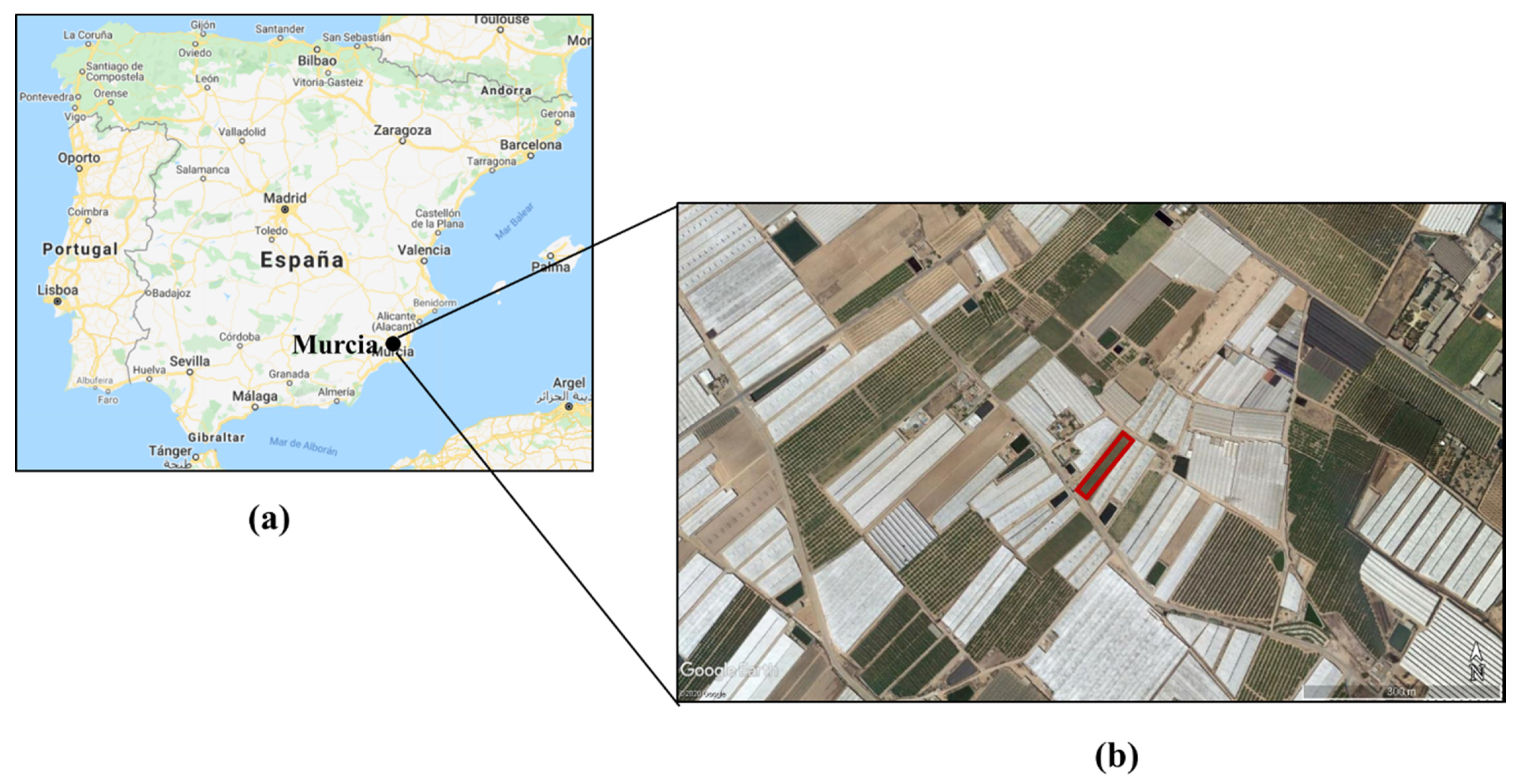
2.1. Study Area

The experiment was conducted during 2019 and 2020 in a commercial bell pepper plot (Capsicum annuum L. var. Maestral), located in San Javier in the Murcia region in the southeast of Spain (Figure 1a), with the geographic coordinates 37°51′11.80″ N latitude and 0°49′50.00″ W longitude and an altitude of 15 m.a.s.l. (meters above the soil level). The experimental plot was an open field, and the area around the plot was dominated by greenhouses. The plot is highlighted in red in Figure 1b. The predominant climate in the study area has been identified as Mediterranean subdesert, with maximum and minimum temperatures of 39.6 and 12.9 °C, respectively, and an average annual rainfall of 313 mm [2].

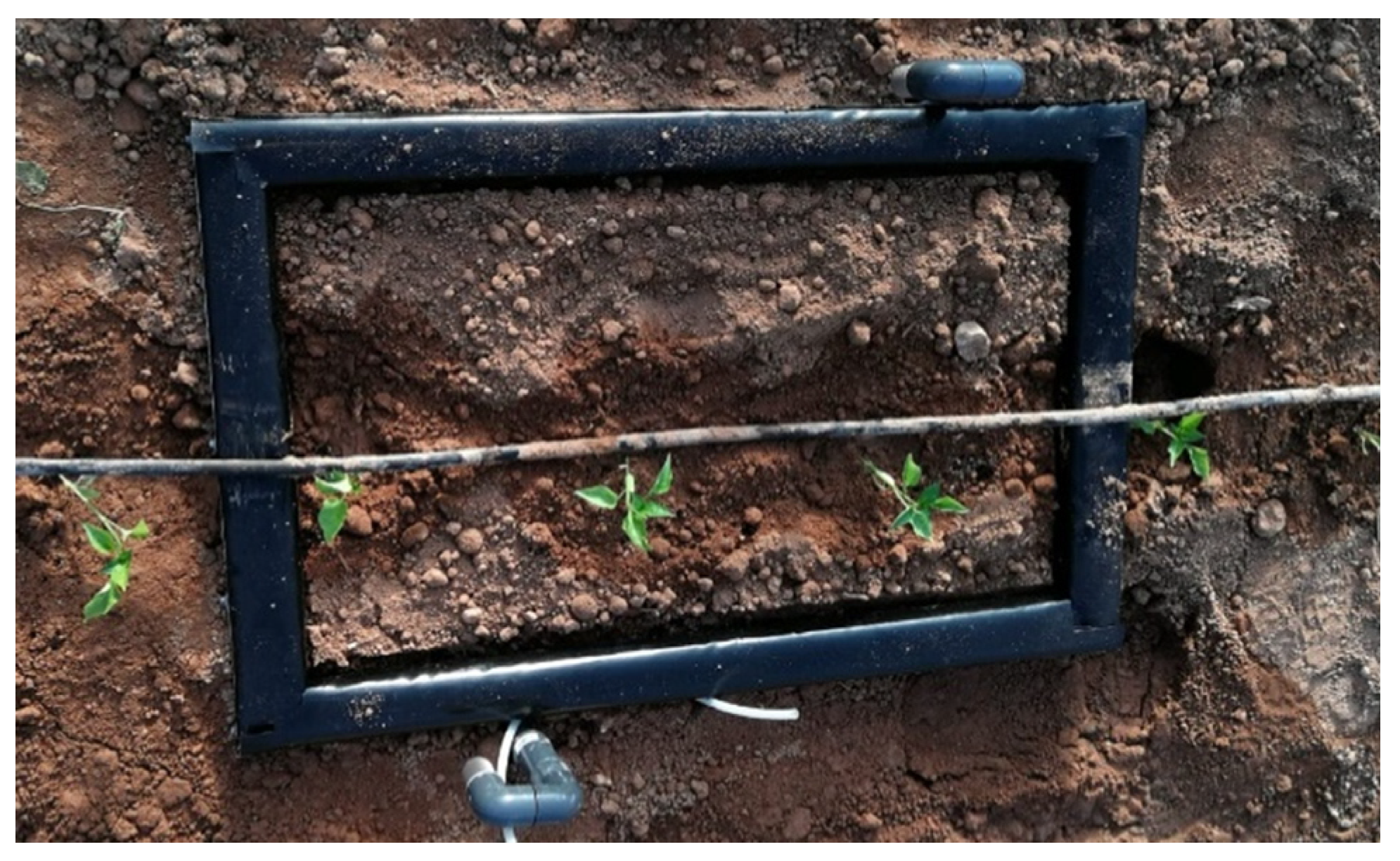
2.2. Description of the Removable Weighing Lysimeter

The removable weighing lysimeter consists of two recipients. One of them is the cultivation recipient (CR) that contains the soil profile and the crop. It has the dimensions of 0.56 × 0.96 × 0.30 m with a small slope at the bottom along all four sides of the container, so that the drained water is guided by gravity to a central hole at the bottom to avoid water accumulation. The second is the drainage recipient (DR) that stores the water that vertically drains from the CR, similar to the one used by Nicolás Cuevas et al. [31].
The lysimeter was installed in the center of the plot, avoiding the edges, because it was necessary that it be surrounded by the same crop to obtain reliable measurements [34]. In a previously excavated hole, in which the dimensions of the lysimeter were considered, the soil extracted during the excavation was then placed in the CR, while trying to keep the soil unaltered. A hydrodynamic characterization of the clay soil was performed based on the methodology proposed by the U.S. Department of Agriculture (USDA) [35] with a bulk density of 1.38 g/cm3. The irrigation system used was drip irrigation, with emitters placed every 25 cm and an application rate of 2.2 L/h (Figure 2).

2.3. Crop Management

The bell pepper crop (Capsicum annuum L.), previously sowed under greenhouse conditions, was transplanted at 10 cm height. The planting frame measured 1 m between lines and 0.33 m between plants, leaving a total of three plants and three drippers within the CR (Figure 2). The vegetative cycle until the harvest was 195 days. The irrigation scheduling was performed following the E T C computation with the lysimeter and with 91% application efficiency.
The fertilization dose was applied with the irrigation water according to the recommendations of the Ministry of Agriculture, Fisheries and Food of Spain [36]; meanwhile, weeds and pests were managed according to the common practices in the agricultural area.

2.4. Determination of Evapotranspiration and Crop Coefficients

The computation of evapotranspiration started with the crop transplanting. Then, through the application of irrigation, the soil reached field capacity, with the initial value of CR representing the soil mass plus water mass plus the mass of three plants. During the crop development, if the soil did not receive water, the CR mass decreased because of the E T C . When irrigation was applied or rainfall occurred, the RC’s mass increased rapidly; if the soil field capacity was exceeded, the soil began to drain or discharge the excess water from the bottom of the RC, which was reflected by the increased mass of the DR. Once irrigation or rainfall was stopped, the soil lost water because of the E T C .
From the operation behavior of the lysimeter described above, the daily crop evapotranspiration was calculated by applying the water balance equation [37] and the conditions established in the work of Peters et al. [28], as in Equations (1) and (2):
E T C L Y S = I Δ DR ± Δ CR
Under conditions of no rain or irrigation water, Equation (1) would be as follows:
E T C L Y S = Δ CR Δ DR
where I is the irrigation depth (mm), ΔCR is the mass variation in the cultivation recipient (mm), and ΔDR in the mass increase in the drainage recipient (mm), considering that 1 kg of lysimeter variation represents 1.85 mm of water.
From the data obtained with the lysimeter, the daily values of the crop coefficient ( K C l y s ) were calculated using Equation (3) [12]:
K C l y s = E T C L Y S E T O
where E T O is the reference evapotranspiration estimated by the FAO Penman–Monteith method [12], considering the climate records generated in an automatic weather station built with a datalogger (CR10X model, Campbell Scientific, Logan, UT, USA), a pyranometer (CM14 model, KIPP&ZONEN Delft), temperature and relative humidity sensors placed at 1.5 m above the ground level (MP100 probe, Campbell Scientific, Logan, UT, USA), anemometer and anemovelta at a 2 m height (A100R and W200P models, respectively, of Vector Instruments Ltd., Rhyl, North Wales, UK), and a rain gauge (ARG100 model, Campbell Scientific, Logan, UT, USA). The automatic weather station was installed next to the weighing lysimeter. The phenological stages were defined according to the Allen et al. [12]’s recommendations.
The E T C value determined with the FAO-56 method [12] was compared with the E T C obtained with the lysimeter, and the model used was as follows:
E T C F A O = E T O × K C F A O
where K C F A O refers the values proposed by the FAO-56 for bell pepper for the different stages of crop development.
From the average air temperature obtained with the weather station, the crop thermal units ( T U ) were determined for the whole cycle [14] by considering a 10 °C basal temperature ( T b ), proposed by Vidal [38], which is the minimum temperature at which the bell pepper can develop.
If   T a > T b :        T U i = ( T a T b ) i If   T a T b : T U i = T U i 1
where T U i is the thermal unit for day i (°C), T U i 1 is the thermal unit for day i 1 (°C), and T a is the average air temperature in (°C) for day i .
The T U values were converted to accumulated fraction thermal units ( F T U ):
F T U i = T U i Σ T U i
where Σ T U i is the total accumulative T U for optimal growth of the bell pepper, proposed by Vidal to be 2200 ± 220 °C [38]. In this experiment, the total cumulative thermal units for the 2019 and 2020 seasons were 1860 and 1904 °C, respectively. A relationship was obtained for the F T U results and the crop coefficient from the lysimeter using the least squares algorithm [39].
Different metrics were used to compare the results obtained from the different methodologies, such as the mean estimation error ( MEE ), the root mean square error ( RMSE ), the systematic mean square error ( MSE s ), the coefficient of determination ( R 2 ), and the index of agreement ( IA ).
MEE = 1 n i = 1 n Y i Y ^ i
RMSE = 1 n i = 1 n ( Y i Y ^ i ) 2
MSE s = 1 n i = 1 n ( Y ^ i Y i ) 2
IA = 1 i = 1 n ( y Y ^ i ) 2 i = 1 n ( | Y ^ y ¯ | + | y y ¯ | ) 2
where n is the data number, Y i is the value measured of i , Y ^ i is the estimated value in the regression of day i or value to be compared, and y ¯ is the mean of the measured values of day i [40,41].

2.5. Water Productivity

According to the methodology proposed by Playán and Mateos [42], the water productivity was determined by the relationship between the production obtained and the volume consumed, expressed in kg/m3, which related to the crop yield per cultivated area in t/ha and the economic benefits per cultivated area, EUR/ha.

3. Results and Discussion

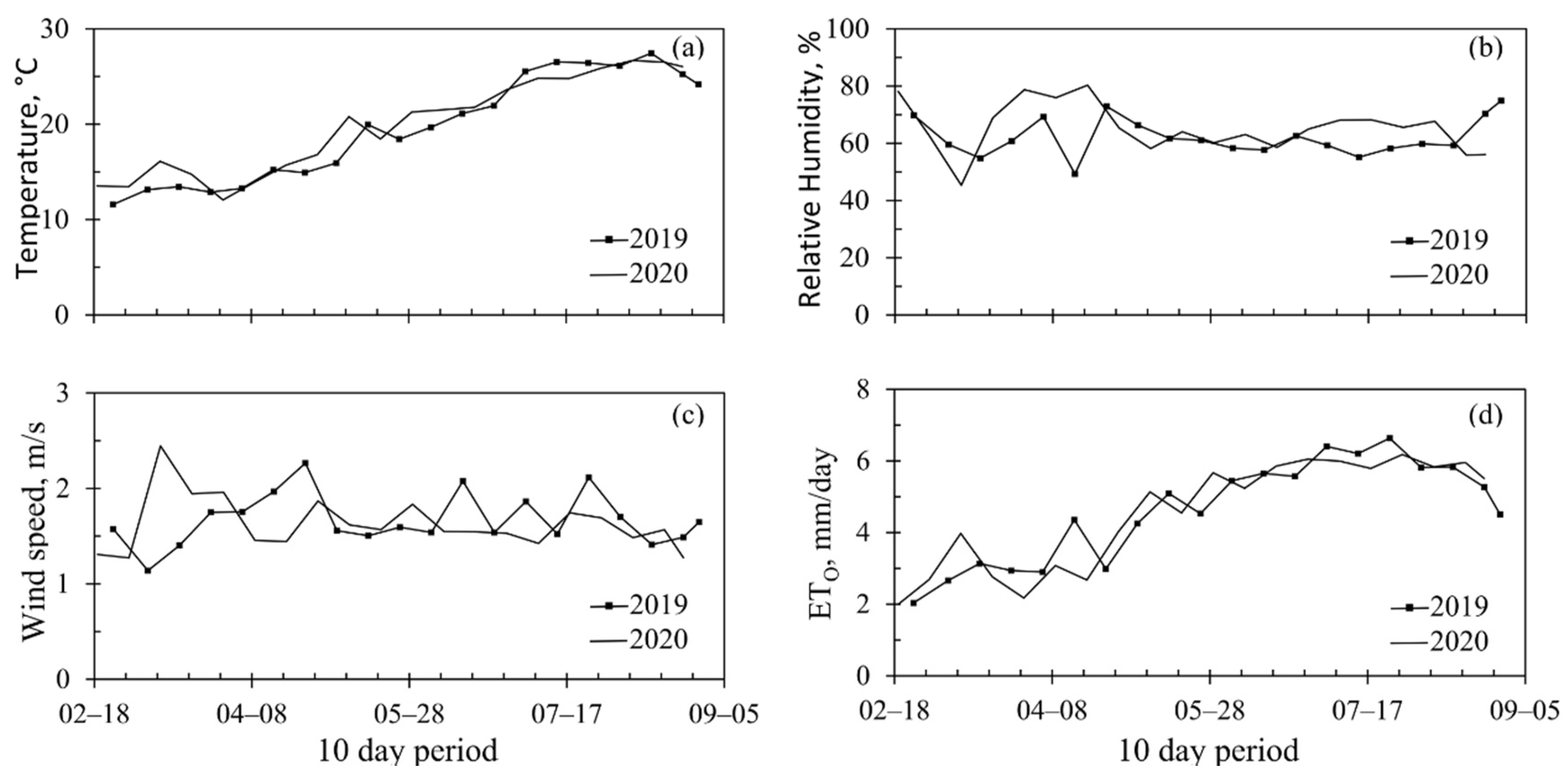
3.1. Meteorological Conditions

The 2019 growing season was from 15 February to 28 August, while the 2020 season was from 10 February to 22 August, both from the date of transplant. The 2019 and 2020 average air temperature, average relative humidity, average wind speed, and E T O for the different periods are shown in Figure 3. The behavior of the climatic variables was very similar for the two seasons. Comparing the two years, March, the end of April, and the first days of June were warmer in 2020, while late June and early July were warmer in 2019.
The relative humidity and wind speed were lower in 2019 than in 2020 for most of the growing season. The relative humidity was especially lower from 14 March to 18 April and from 27 July to 10 August in 2020. The average relative humidity values recorded for the two seasons were greater than 60%, with minimum and maximum averages of 47.31% and 76.61%, respectively. The average wind speed was 1.67 m/s in 2019 and 1.65 m/s in 2020. The E T O increased in a similar manner to the ambient temperature, with the average E T O being 4.6 mm/day in 2019 and 4.6 mm/day in 2020.

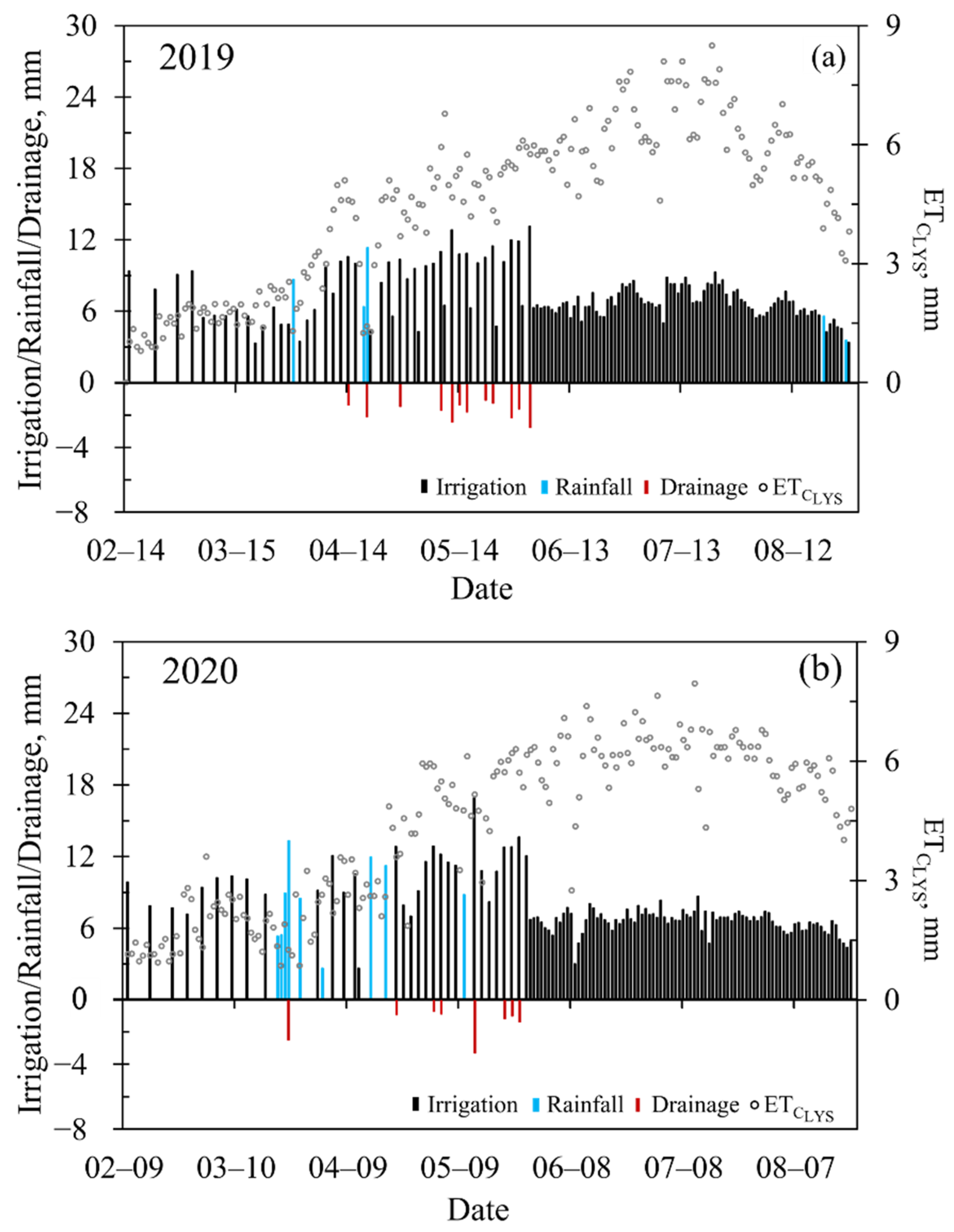
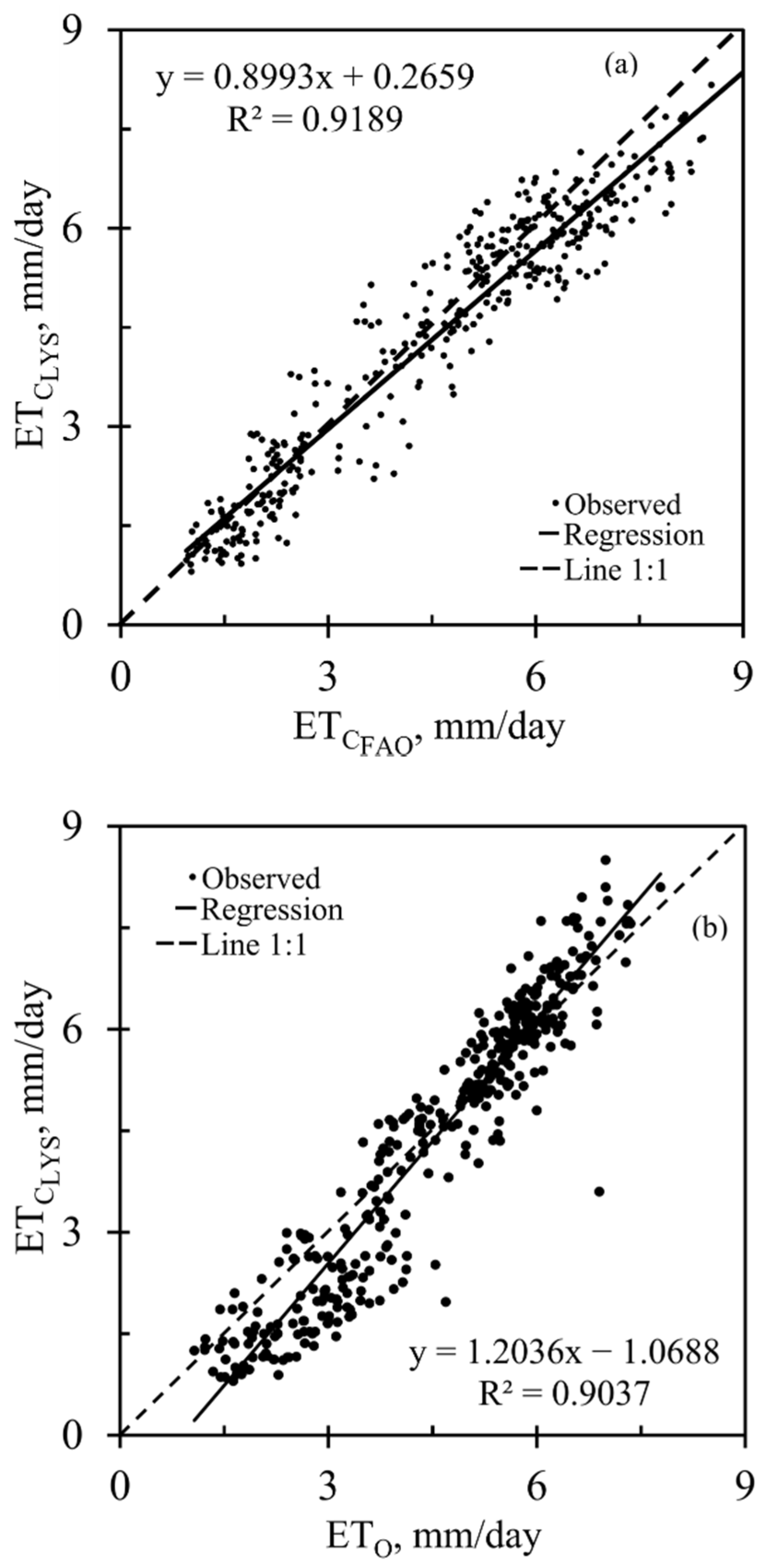
3.2. Crop Evapotranspiration

Figure 4 shows the daily values of the E T C of the crop, the inputs due to rain and/or irrigation, and the water losses by drainage. Initially, irrigation was applied every three days on average; however, according to the crop growth and an increase in E T C as a result of high summer temperatures, the schedule changed to every two days, then decreased again to one day between irrigations.
The irrigation intervals showed a similar trend in both seasons; the widest interval between irrigations for the 2019 season was five days and extended only until February, while for the 2020 season, the widest interval was three days on average and extended until 20 April. In April, the E T C increased, causing the interval to decrease to two days. In the days at the end of May, when summer started, irrigation took place daily. In this period, the daily evapotranspiration of the crop was higher than 5 mm. This interval started earlier in the 2020 season. The total application of irrigation was 960.3 mm in 2019 and 936.1 mm in 2020. In 2020, there were more rainfall events and therefore less irrigation was applied, with 40.7 mm more rain and double the number of events, meaning 2.52% less irrigation applied.
Table 1 shows the average values for irrigation, rainfall, drainage, and evapotranspiration for both years.
Comparing the gross depth of irrigation obtained with the lysimeter to that obtained with the FAO-56 methodology, a decrease of 1.33% was found in 2019 because the water depth was 947.6 mm with FAO. In 2020, the water depth was 928.8 mm, representing a decrease of 0.78% with respect to the lysimeter measurements. These decreases were small, and the difference in depth can mean just one or two irrigations. The drainages reported by the lysimeter achieved an average of 12 mm, with 12 and 14 events for the 2019 and 2020 seasons, respectively. In the first season, the drainages did not exceed 4 mm and were caused by the irrigations that came to exceed a 10 mm depth; for instance, the drainage caused by the rains on 19–21 April with a 28.4 mm depth. In the second season, one of the drainages was caused by rain on 21–24 March of 33 mm in depth and the others were caused by an irrigation depth larger than 12 mm. The major rainfall events were in the months of March and April; for the first year, there were five days of rain with an accumulated depth of 35.4 mm, while in the second year, there were double the number of days and an accumulated depth of 76.1 mm.
The E T C increased when the temperature increased and the interval between irrigations decreased, indicating the relationship that E T C has with both variables. The maximum E T C value was reached close to 16 July for the both seasons. When the irrigation application was on a daily scale, the E T C had high values above 5 mm. The behavior of the E T C during rainy days was small, and it was larger the day after irrigation or rain because the evaporation of the wet soil was more significant; in this same context, in the days when no irrigation was performed, due to longer intervals, the E T C was maintained or declined, because there is less evaporation from a soil with a dry surface [12]. The total E T C for the 2019 and 2020 seasons were 874.4 mm and 854.6 mm, respectively.
The lysimeter-measured E T C L Y S values for both seasons were compared to the E T O calculated using the Penman–Monteith method and the E T C obtained using the method established by the standard methodology of FAO-56 ( E T C F A O ) [12], presented in Figure 5. The resulting average E T C L Y S values for the initial, middle, and final stages were 1.6, 5.8, and 5.4 mm/day, respectively.
The linear correlation between E T C L Y S and E T O showed a good agreement (Figure 5b). The determination coefficient was 0.90 and the RMSE was 1.04 mm/day for both seasons, indicating the dependence that exists between the variables. In the comparison of E T C L Y S and E T C F A O , the linear regression slope was close to unity and the RMSE was 0.63 mm/day. The values of E T C F A O in the whole crop cycle overestimated the E T C L Y S by 37.44%, with an average value of 0.4 mm/day; this may be due to the fact that the K C values used in the FAO-56 methodology were standard values calibrated under different conditions than those of this experiment.
The MEE was close to zero (0.03 mm/day in 2019 and 0.01 mm/day in 2020), indicating a low bias between E T C L Y S and E T C F A O . Similarly, the other metrics showed the same behavior. The IA values were close to one (0.98 in 2019 and 0.98 in 2020), indicating a good agreement with both E T C models. However, the MSE S values were 4.05% in 2019 and 3.91% in 2020, indicating high bias, meaning one of the methods should be improved. The MSE S obtained by Martínez-Cob [14] are very similar to the results of this research, with both MSE S being greater than two.

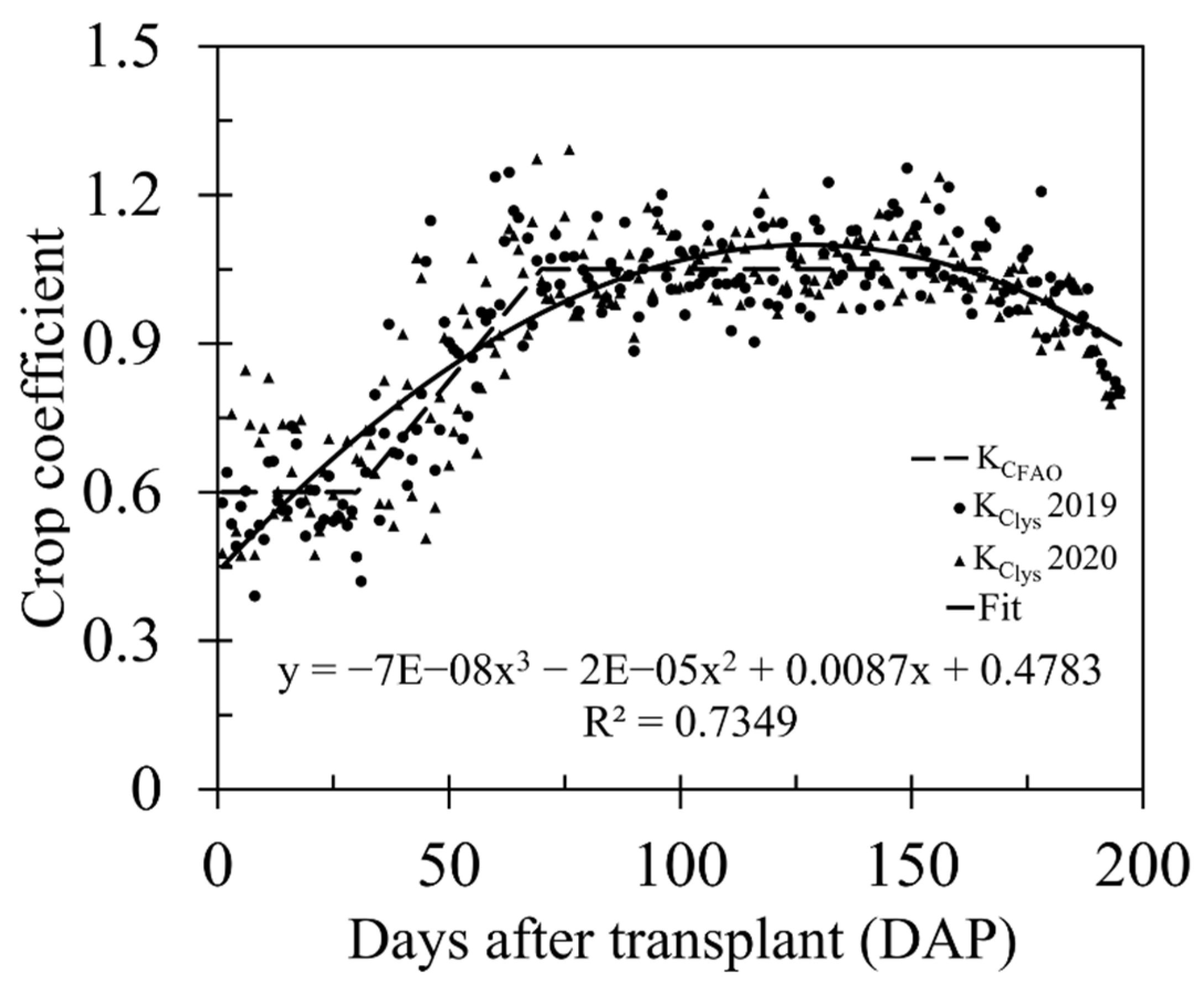
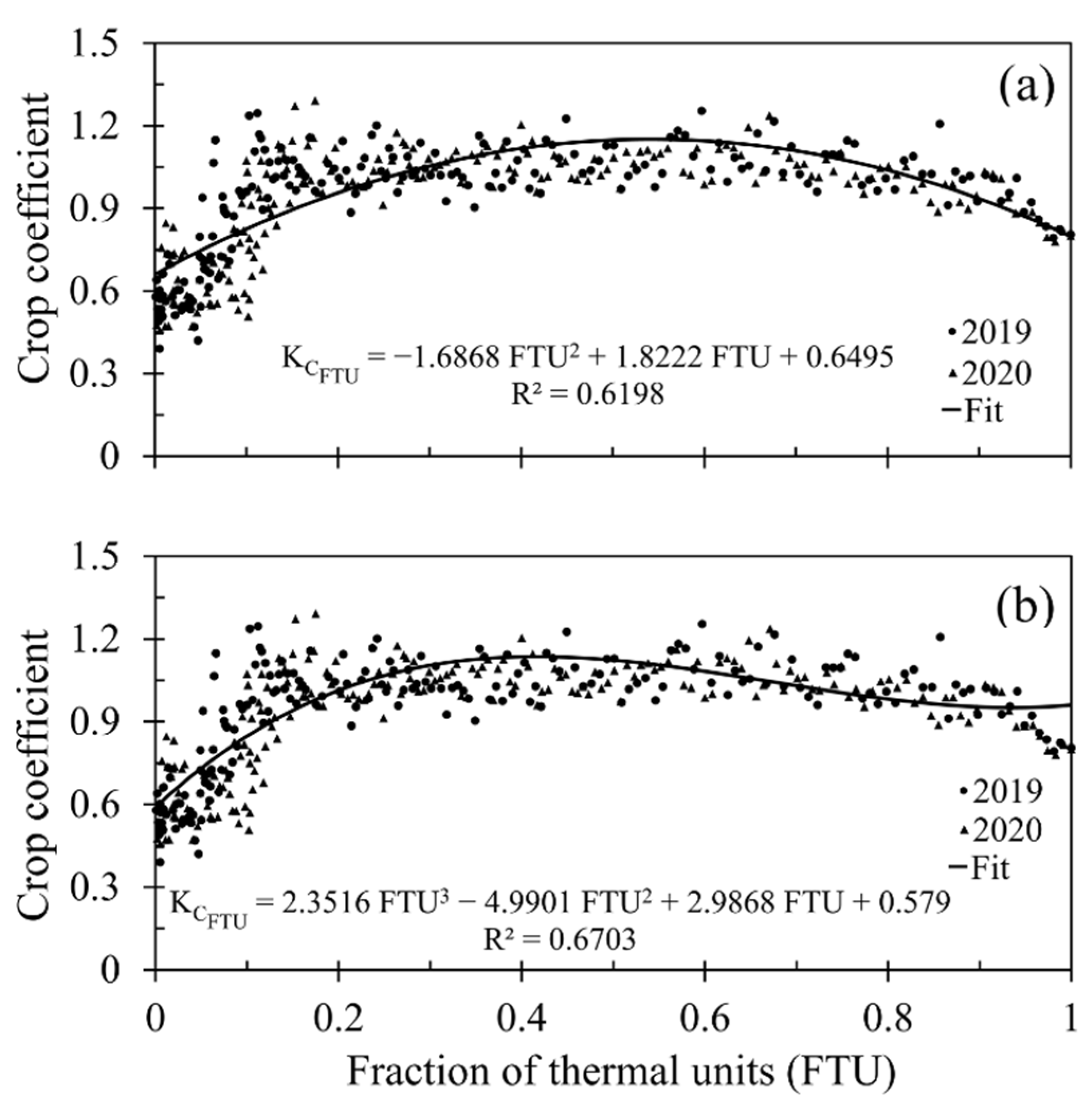
3.3. Crop Coefficient

The crop coefficient values estimated from Equation (3) ( K C l y s ) and the values established in the FAO-56 paper for this crop ( K C F A O ) are show in Figure 6. The K C l y s   i n i of the lysimeter was 0.57, K C l y s   m i d was 1.06, and K C l y s   e n d was 0.80. These data were adjusted to a third-degree polynomial curve, with an R 2 of 0.73. In this model, a maximum K C of 1.11 and a minimum of 0.48 were observed.
When comparing K C l y s to K C F A O , an R 2 of 0.79 and an RMSE of 0.09 were obtained. The values of K C l y s oscillated around the values recommended by Allen et al. [12].
The jump in K C l y s between DAP 50 and 75 (Figure 6) may be due to the low reference evapotranspiration values reported on those days in both seasons, being more significant for the 2020 season. It should be remembered that in Equation (3), K C l y s is a function of E T O , so the lower the E T O , the higher the K C l y s .
A relationship between K C l y s and the fraction thermal units ( F T U ) was obtained; Figure 7 shows the two resulting graphs of the polynomial fit. As shown in Figure 7a, the maximum K C F T U value was 1.15 for the F T U range of 0.43–0.62; the maximum for Figure 7b was 1.15 in the range of 0.36–0.49. Although, the second setting (Figure 7b) showed a slightly better R 2 , it reached a maximum curve during the early F T U period and a slower decrease; the curve at the end of the cycle rose and moved away from the observed points.
The average total of F T U was 1881.76, a value in the range proposed by Vidal [38]. There was a lower bias between K C F A O and K C F T U , followed by K C F A O against K C l y s with 0.09 and K C F T U against K C l y s with 0.48. These values are shown in Table 2.
Table 2 shows the K C values of two works that estimated the K C values for the bell pepper. The work of Shukla et al. [43] was performed in Florida, USA during the 2003–2008 fall–winter seasons, with a temperature range of 17–29 °C, an annual rainfall of 1260 mm/year, a total E T C of 267 mm, and with a high water table. The crop bed was covered with plastic mulch that covered 33% of the lysimeter area.
In the area of Peninsular Malaysia, characterized by a warm and humid climate, the second study was performed by Muniandy et al. [44] during August 2013 and May 2014, with an average temperature range of 24–30 °C, a monthly rainfall of 125–270 mm, and relative humidity (RH) between 63% and 88%. Both investigations used the same methodology to determine the E T C and K C as used in this study.
The temperature range and the relative humidity of both works were in the same range as our work, but with higher rainfalls than those registered in a whole year in our study zone and performed in a different sowing season. Shukla et al. [43] reported high bimonthly values of E T C for their seasons, because irrigation and rainfall kept the groundwater table high and increased the soil moisture with mulching. Therefore, the K C values of this research were the highest (Table 1); they were 50.88%, 14.15%, and 60% higher in each stage, respectively, compared to values reported with the lysimeter in this research.
In contrast, the values of Muniandy et al. [44] in the middle and final stages were the lowest, as shown in Table 2. The climatic conditions were very similar to those of the work mentioned above, but without the influence of the water table. These values presented a reduction of 10.38% and 5% in K C m i d and K C e n d , respectively, from those reported in this work with the lysimeter. The values proposed by Allen et al. [12] presented less variability with respect to those obtained with the lysimeter in this research, with an increase in the initial and final stages of 5.26% and 12.5%, respectively, and a decrease in the middle stage of 0.94%. The FAO values pertain to climates with a RH close to 45% and wind speeds close to 2 m/s; our conditions satisfy these figures.

3.4. Yield

Table 3 shows a summary of the final production achieved in each season. The bell pepper yield for both seasons was superior to that reported by the Ministry of the Environment and Rural and Marine Areas of the Spanish Government in 2019 of 75.66 t/ha for the Region of Murcia [6]. The removable weighing lysimeter allowed greater precision in the control of the crop water balance, which increased the crop yield and produced a significant water saving in comparison to the common practices of the Region of Murcia. The water production and economic yields were similar for both seasons.
In 2019, a better yield was obtained, as the excess humidity in the soil caused by the rains in 2020 generated an abortion of flowers, reducing the productivity of the bell pepper in that year [45].

4. Conclusions

The E T C and K C values for the bell pepper crop were calculated using a compact weighing lysimeter and an automatic weather station for two seasons in the semiarid southeast of Murcia, Spain. The E T C was affected by irrigation and rainfall events, which increased the soil evaporation, most notably when there was a shorter interval between irrigations. Second- and third-order models were developed for K C as a function of fraction thermal units, based on the data of K C inferred from the lysimeter with determination coefficients greater than 0.60. The average values of K C for the bell pepper for the initial, middle, and final stages were 0.57, 1.06, and 0.80, respectively. The K C values were similar to those proposed by Allen et al. [12] because the climatic conditions were similar in both studies, which were lower compared to the values of Shukla et al. [43], where the climatic conditions were similar but the rain and the contribution of the water table caused greater evaporation.
An increase in the bell pepper yield of 7.72% in 2019 and of 3.49% in 2020 was achieved compared to the yield established by the Ministry of the Environment and Rural and Marine Areas of the Spanish Government [6]. The K C l y s values and the F T U models for the bell pepper obtained in this study will help farmers to determine the water requirement and to improve the crop water efficiency in semiarid locations with conditions similar to those of this study.

Author Contributions

Conceptualization and methodology L.Á.-D., J.M.M.-M., and C.B.-C.; validation and formal analysis, L.Á.-D., J.M.M.-M., C.B.-C., M.S.-M., and J.G.-T.; investigation and resources, M.S.-M., H.E.J.-F., C.O.R.R., and J.G.-T.; writing—original draft L.Á.-D., J.M.M.-M., and C.B.-C.; writing—review and editing, M.S.-M., H.E.J.-F., C.O.R.R., and J.G.-T.; visualization and supervision, L.Á.-D., J.M.M.-M., C.B.-C., M.S.-M., and J.G.-T.; project administration and funding acquisition, J.M.M.-M., and M.S.-M. All authors have read and agreed to the published version of the manuscript.

Funding

This research was financed by the Project of Research and Development, reference IDI-20190146, titled “Development and implementation of a ferticontrol equipment by weighing lysimetry for use in intensive agriculture,” in collaboration with the AGROSOLMEN, S.L. company, co-financed by the European Regional Development Fund (FEDER) through the Spanish Pluri-Regional Operational Programme 2014–2020.

Institutional Review Board Statement

Not applicable.

Informed Consent Statement

Not applicable.

Data Availability Statement

No new data were created or analyzed in this study. Data sharing is not applicable to this article.

Acknowledgments

The authors acknowledge CONACyT for the grant provided to L.A.-D. for her PhD studies.

Conflicts of Interest

The authors declare no conflict of interest.

References

  1. Fernández-Pacheco, D.G.; Escarabajal-Henarejos, D.; Ruiz-Canales, A.; Conesa, J.; Molina-Martínez, J.M. A digital image-processing-based method for determining the crop coefficient of lettuce crops in the southeast of Spain. Biosyst. Eng. 2014, 117, 23–34. [Google Scholar] [CrossRef]
  2. Escarabajal-Henarejos, D.; Molina-Martínez, J.M.; Fernández-Pacheco, D.G.; Cavas-Martínez, F.; García-Mateos, G. Digital photography applied to irrigation management of Little Gem lettuce. Agric. Water Manag. 2014, 151, 148–157. [Google Scholar] [CrossRef]
  3. López-Urrea, R.; Montoro, A.; López-Fuster, P.; Fereres, E. Evapotranspiration and responses to irrigation of broccoli. Agric. Water Manag. 2009, 96, 1155–1161. [Google Scholar] [CrossRef]
  4. Egbuikwem, P.N.; Obiechefu, G.C. Evaluation of Evapotranspiration Models for Waterleaf crop using Data from Lysimeter. In Proceedings of the 2017 Spokane, Washington, DC, USA, 16–19 July 2017; American Society of Agricultural and Biological Engineers: St. Joseph Charter Township, MI, USA, 2017. [Google Scholar]
  5. Yimam, A.Y.; Assefa, T.T.; Adane, N.F.; Tilahun, S.A.; Jha, M.K.; Reyes, M.R. Experimental Evaluation for the Impacts of Conservation Agriculture with Drip Irrigation on Crop Coefficient and Soil Properties in the Sub-Humid Ethiopian Highlands. Water 2020, 12, 947. [Google Scholar] [CrossRef] [Green Version]
  6. Ministerio de Medio Ambiente y Medio Rural y Marino Estadísticas Agrarias. Available online: https://www.mapa.gob.es/es/estadistica/temas/estadisticas-agrarias/ (accessed on 15 October 2020).
  7. Nikolaou, G.; Neocleous, D.; Christou, A.; Kitta, E.; Katsoulas, N. Implementing Sustainable Irrigation in Water-Scarce Regions under the Impact of Climate Change. Agronomy 2020, 10, 1120. [Google Scholar] [CrossRef]
  8. González-Esquiva, J.M.; García-Mateos, G.; Escarabajal-Henarejos, D.; Hernández-Hernández, J.L.; Ruiz-Canales, A.; Molina-Martínez, J.M. A new model for water balance estimation on lettuce crops using effective diameter obtained with image analysis. Agric. Water Manag. 2017, 183, 116–122. [Google Scholar] [CrossRef]
  9. Feltrin, R.M.; de Paiva, J.B.D.; de Paiva, E.M.C.D.; Beling, F.A. Lysimeter soil water balance evaluation for an experiment developed in the Southern Brazilian Atlantic Forest region. Hydrol. Process. 2011, 25, 2321–2328. [Google Scholar] [CrossRef]
  10. Soldevilla-Martinez, M.; Quemada, M.; López-Urrea, R.; Muñoz-Carpena, R.; Lizaso, J.I. Soil water balance: Comparing two simulation models of different levels of complexity with lysimeter observations. Agric. Water Manag. 2014, 139, 53–63. [Google Scholar] [CrossRef]
  11. Cunha, H.; Loureiro, D.; Sousa, G.; Covas, D.; Alegre, H. A comprehensive water balance methodology for collective irrigation systems. Agric. Water Manag. 2019, 223, 105660. [Google Scholar] [CrossRef]
  12. Allen, R.G.; Pereira, L.S.; Raes, D.; Smith, M. Crop Evapotranspiration-Guidelines for Computing Crop Water Requirements-FAO Irrigation and Drainage Paper 56; FAO: Rome, Italy, 1998; Volume 300. [Google Scholar]
  13. Sepaskhah, A.R.; Andam, M. Crop coefficient of sesame in a semiarid region of IR Iran. Agric Water Manag. 2001, 49, 51–63. [Google Scholar] [CrossRef]
  14. Martínez-Cob, A. Use of thermal units to estimate corn crop coefficients under semiarid climatic conditions. Irrig. Sci. 2008, 26, 335–345. [Google Scholar] [CrossRef] [Green Version]
  15. Mateos, L.; González-Dugo, M.P.; Testi, L.; Villalobos, F.J. Monitoring evapotranspiration of irrigated crops using crop coefficients derived from time series of satellite images. I. Method validation. Agric. Water Manag. 2013, 125, 81–91. [Google Scholar] [CrossRef]
  16. Kullberg, E.G.; DeJonge, K.C.; Chávez, J.L. Evaluation of thermal remote sensing indices to estimate crop evapotranspiration coefficients. Agric. Water Manag. 2017, 179, 64–73. [Google Scholar] [CrossRef] [Green Version]
  17. Vaughan, P.J.; Trout, T.J.; Ayars, J.E. A processing method for weighing lysimeter data and comparison to micrometeorological ETo predictions. Agric. Water Manag. 2007, 88, 141–146. [Google Scholar] [CrossRef]
  18. Evett, S.R.; Mazahrih, N.T.; Jitan, M.A.; Sawalha, M.H.; Colaizzi, P.D.; Ayars, J.E. A Weighing Lysimeter for Crop Water Use Determination in the Jordan Valley, Jordan. Trans. ASABE 2009, 52, 155–169. [Google Scholar] [CrossRef]
  19. Bello, Z.A.; Van Rensburg, L.D. Development, calibration and testing of a low-cost small lysimeter for monitoring evaporation and transpiration: Development, calibration and testing of a low cost small lysimeter. Irrig. Drain. 2017, 66, 263–272. [Google Scholar] [CrossRef]
  20. Benli, B.; Kodal, S.; Ilbeyi, A.; Ustun, H. Determination of evapotranspiration and basal crop coefficient of alfalfa with a weighing lysimeter. Agric. Water Manag. 2006, 81, 358–370. [Google Scholar] [CrossRef]
  21. Anapalli, S.S.; Ahuja, L.R.; Gowda, P.H.; Ma, L.; Marek, G.; Evett, S.R.; Howell, T.A. Simulation of crop evapotranspiration and crop coefficients with data in weighing lysimeters. Agric. Water Manag. 2016, 177, 274–283. [Google Scholar] [CrossRef] [Green Version]
  22. Wegehenkel, M.; Zhang, Y.; Zenker, T.; Diestel, H. The use of lysimeter data for the test of two soil-water balance models: A case study. Z. Pflanzenernähr. Bodenk. 2008, 171, 762–776. [Google Scholar] [CrossRef]
  23. Meissner, R.; Seeger, J.; Rupp, H.; Seyfarth, M.; Borg, H. Measurement of dew, fog, and rime with a high-precision gravitation lysimeter. J. Plant Nutr. Soil Sci. 2007, 170, 335–344. [Google Scholar] [CrossRef]
  24. Schrader, F.; Durner, W.; Fank, J.; Gebler, S.; Pütz, T.; Hannes, M.; Wollschläger, U. Estimating Precipitation and Actual Evapotranspiration from Precision Lysimeter Measurements. Procedia Environ. Sci. 2013, 19, 543–552. [Google Scholar] [CrossRef] [Green Version]
  25. Herbrich, M.; Gerke, H.H. Autocorrelation analysis of high resolution weighing lysimeter time series as a basis for determination of precipitation. J. Plant Nutr. Soil Sci. 2016, 179, 784–798. [Google Scholar] [CrossRef]
  26. Hannes, M.; Wollschläger, U.; Schrader, F.; Durner, W.; Gebler, S.; Pütz, T.; Fank, J.; von Unold, G.; Vogel, H.-J. A comprehensive filtering scheme for high-resolution estimation of the water balance components from high-precision lysimeters. Hydrol. Earth Syst. Sci. 2015, 19, 3405–3418. [Google Scholar] [CrossRef] [Green Version]
  27. Hoffman, M.; Schwartengräber, R.; Wessolek, G.; Peters, A. Comparison of simple rain gauge measurements with precision lysimeter data. Atmos. Res. 2016, 174–175, 120–123. [Google Scholar] [CrossRef]
  28. Peters, A.; Nehls, T.; Schonsky, H.; Wessolek, G. Separating precipitation and evapotranspiration from noise—A new filter routine for high-resolution lysimeter data. Hydrol. Earth Syst. Sci. 2014, 18, 1189–1198. [Google Scholar] [CrossRef] [Green Version]
  29. Young, M.H.; Wierenga, P.J.; Mancino, C.F. Large Weighing Lysimeters for Water Use and Deep Percolation Studies. Soil Sci. 1996, 161, 491–501. [Google Scholar] [CrossRef]
  30. Ruiz-Peñalver, L.; Vera-Repullo, J.A.; Jiménez-Buendía, M.; Guzmán, I.; Molina-Martínez, J.M. Development of an innovative low cost weighing lysimeter for potted plants: Application in lysimetric stations. Agric. Water Manag. 2015, 151, 103–113. [Google Scholar] [CrossRef]
  31. Nicolás-Cuevas, J.A.; Parras-Burgos, D.; Soler-Méndez, M.; Ruiz-Canales, A.; Molina-Martínez, J.M. Removable Weighing Lysimeter for Use in Horticultural Crops. Appl. Sci. 2020, 10, 4865. [Google Scholar] [CrossRef]
  32. METER Group Smart Field Lysimeter. Available online: https://www.metergroup.com/environment/products/smart-field-lysimeter/%20or/ (accessed on 12 December 2020).
  33. UGT-Team Lysimeter Technology. Available online: https://www.ugt-online.de/en/products/lysimeter-technology/ (accessed on 12 December 2020).
  34. Aboukhaled, A.; Alfaro, A.; Smith, M. Lysimeters. In FAO Irrigation and Drainage Paper 39; Food and Agriculture Organization United Nations: Rome, Italy, 1982. [Google Scholar]
  35. Soil Survey Staff. Soil Survey Manual; United State Department of Agriculture: Washington, DC, USA, 1951. [Google Scholar]
  36. Ministerio de Agricultura, Pesca y Alimentación Guía Práctica de la Fertilización Racional de los Cultivos en España. Available online: https://www.mapa.gob.es/es/agricultura/publicaciones/Publicaciones-fertilizantes.aspx (accessed on 7 February 2019).
  37. Miranda, F.R.; Gondim, R.S.; Costa, C.A.G. Evapotranspiration and crop coefficients for tabasco pepper (Capsicum frutescens L.). Agric. Water Manag. 2006, 82, 237–246. [Google Scholar] [CrossRef]
  38. Vidal, J.L. Efectos del Factor Térmico en el Desarrollo del Crecimiento Inicial de Pimiento (Capsicum annum L.) Cultivado en Campo; Universidad Nacional de Tucumán: Tucumán, Argentina, 2011. [Google Scholar]
  39. Verma, S.P. Análisis Estadístico de Datos Composicionales; Universidad Autónoma de México: Ciudad de México, Mexico, 2016. [Google Scholar]
  40. Wackerly, D.D.; Mendenhall, W.; Schaeaffer, R.L. Mathematical Statics with Applications, 7th ed.; Learning Cengage; Cengage Learning: Boston, MA, USA, 2010. [Google Scholar]
  41. Willmott, C.; Ackleso, S.; Davis, O.; Feddema, J.; Klink, K.; Legate, D.; Rowe, A. Statistics for the Evaluation and Comparison of Models. J. Geophys. Res. Oceans 1985, 90, 8995–9005. [Google Scholar] [CrossRef] [Green Version]
  42. Playán, E.; Mateos, L. Modernization and optimization of irrigation systems to increase water productivity. Agric. Water Manag. 2006, 80, 100–116. [Google Scholar] [CrossRef] [Green Version]
  43. Shukla, S.; Jaber, F.H.; Goswami, D.; Srivastava, S. Evapotranspiration losses for pepper under plastic mulch and shallow water table conditions. Irrig. Sci. 2013, 31, 523–536. [Google Scholar] [CrossRef]
  44. Muniandy, J.M.; Yusop, Z.; Askari, M. Evaluation of reference evapotranspiration models and determination of crop coefficient for Momordica charantia and Capsicum annuum. Agric. Water Manag. 2016, 169, 77–89. [Google Scholar] [CrossRef]
  45. López-Marín, J.; Angosto, J.L.; González, A. El cultivo de pimientos en invernadero y al aire libre. El caso del Campo de Cartagena. Bibl. Hortic. 2017, 1, 1–67. [Google Scholar]
Figure 1. Study area: (a) Region of Murcia and (b) location of the experimental plot.
Sustainability 13 00747 g001
Figure 2. Top view of the compact weighing lysimeter during the experimentation.
Sustainability 13 00747 g002
Figure 3. Average meteorological data for a 10-day period: (a) ambient temperature, (b) relative humidity, (c) wind speed, and (d) reference evapotranspiration ( E T O ).
Sustainability 13 00747 g003
Figure 4. Daily evapotranspiration of the bell pepper measured with the weighing lysimeter ( E T C L Y S ) and irrigation, rainfall, and drainage: (a) 2019 and (b) 2020.
Sustainability 13 00747 g004
Figure 5. Correlation between E T C L Y S measured by the weighing lysimeter and E T C F A O determined by FAO-56 method (a) and between E T C L Y S and   E T O (b).
Sustainability 13 00747 g005
Figure 6. Bell pepper crop coefficients the during the crop cycle (lysimeter and FAO-56 method values).
Sustainability 13 00747 g006
Figure 7. Polynomial fitting of the crop coefficient ( K C ) values obtained for 2019 and 2020: (a) Second-order polynomial fitting and (b) third-order polynomial fitting.
Sustainability 13 00747 g007
Table 1. Seasonal water balance in millimeters.
SeasonIrrigationRainfallDrainage E T C L Y S
2019960.335.412.31874.4
2020936.176.112.03854.6
Table 2. K C values obtained in this study and other works.
K C Values Crop StageLocationIrrigation MethodClimateCrop Cycle
(Day)
InitialMiddleEndConditions
K C l y s 0.571.060.80Murcia, SpainDripTemp. 12–28 °C
RH 47%–77%
Rain <100 mm/season
E T c ≈ 860 mm/season
195
K C F T U *0.691.050.78
K C F T U **0.651.060.93
Allen et al. [12]0.61.050.9Europe and Mediterranean__RH ≈ 45%125
Shukla et al. [43]0.861.211.28Florida, USASub-surfaceTemp. 17–29 °C
Rain 1260 mm/year
E T c 267 mm
100
Muniandy et al. [44]0.670.950.76Kluang, MalaysiaSprinklerTemp. 24–30 °C
Rain 125–270 mm/month
RH 63%–88%
125
* Second-order polynomial fit values; ** third-order polynomial fit values. RH, relative humidity.
Table 3. Production data of both seasons.
YearBell Pepper Yield (t/ha)Water Productivity (Kg/m3)Economic Yield (EUR/ha)
201981.58.4964,457.55
202078.38.3664,808.91
Publisher’s Note: MDPI stays neutral with regard to jurisdictional claims in published maps and institutional affiliations.

