Article

Turbulence Effect of Urban-Canopy Flow on Indoor Velocity Fields under Sheltered and Cross-Ventilation Conditions

1
Malaysia-Japan International Institute of Technology, Universiti Teknologi Malaysia, Kuala Lumpur 54100, Malaysia
2
Faculty of Engineering Sciences, Kyushu University, Fukuoka 816-8580, Japan
*
Authors to whom correspondence should be addressed.
Sustainability 2021, 13(2), 586; https://doi.org/10.3390/su13020586
Submission received: 1 December 2020 / Revised: 30 December 2020 / Accepted: 7 January 2021 / Published: 9 January 2021
(This article belongs to the Special Issue Sustainable Urban Environment and Building Energy Efficiency)

Abstract

:
Understanding the characteristics of natural, wind-induced ventilation of buildings is essential for accurate predictions of ventilation flow rates; however, indoor ventilation is significantly influenced by surrounding buildings. Therefore, a series of wind-tunnel experiments were performed to clarify the relationship between outdoor and indoor air flows around and within a target cube model with several openings. Two surrounding building arrangements, namely square (SQ) and staggered (ST), were placed under the condition of a building coverage ratio of 25%. The results indicated that the wind speed near the windward openings on the streamwise faces showed 0.3 to the reference wind speed, whereas those on the lateral faces were less than 0.1; these numbers indicate that the opening positions significantly affect the mean indoor wind speed. Furthermore, the temporal fluctuations of velocities near the opening demonstrated that the introduction of the flow is significantly affected by turbulent flow due to the surrounding buildings. In addition, correlation between the outdoor and indoor air flows was observed. The highest correlations were obtained for both opening conditions with a certain temporal delay. This result indicates that indoor air flows become turbulent because of the turbulent flows generated by the surrounding outdoor buildings; however, slight temporal delays could occur between indoor and outdoor air flows. Although the present study focuses on the fundamental turbulent characteristics of indoor and outdoor air flows, such findings are essential for accurately predicting the ventilation flow rate due to turbulent air flows for sheltered buildings.

1. Introduction

Utilizing wind-induced, natural ventilation is a passive method to reduce the energy consumption associated with mechanical ventilation and air-conditioning load. Generally, dependence on mechanical ventilation can be reduced when indoor spaces are naturally ventilated. To adequately utilize natural ventilation, assessing the factors that influence the ventilation rate of a building is essential. For example, natural ventilation rates depend on various factors such as the shape of the target building, opening condition, and wind direction [1,2]. Studies on indoor air-flow fields for natural ventilation include numerical simulations [3,4,5,6] and experiments [7,8,9,10].
Numerous studies have investigated the indoor air flow of isolated buildings. For example, Asfour and Gadi [2] adopted the computational fluid-dynamics (CFD) approach and applied a mathematical model to predict the air-flow rate for the cross-ventilation of an isolated model exposed to perpendicular and oblique wind directions. Bangalee et al. [11] adopted both wind-tunnel experimentation and CFD to compare the flow patterns from the inlet to the outlet of a cube model. To improve the prediction of air-flow rates for building ventilation, Shirzadi et al. [12] proposed a discharge coefficient, which is a function of the building geometry and opening position. Essentially, previous studies have demonstrated the significance of the introduction of air through the windward opening in relation to the efficiency of cross-ventilation in unsheltered models.
However, the presence of surrounding buildings tends to influence the wind flow in the vicinity of a target building, and this is the typical configuration of an urban residential area. To elucidate the mechanism of ventilation so it reflects the real world, it is necessary to conduct research on the indoor air flow of buildings by considering the presence of surrounding buildings. In fact, it was discovered that changes in a building’s inflow of air due to the presence of surrounding buildings may greatly change the average indoor air flow and turbulent flow-intensity distribution [13], which has a great effect on the mixing of air inside the room. The dependence of the air flow properties inside the buildings on the arrangement conditions of the surrounding buildings was also supported by the wind-tunnel experiments of Hasegawa [14]. In addition, the CFD studies by Kasim et al. [5] and Zaki et al. [6] focused on the internal flow of a building with cross-ventilation, and showed that the mean wind flow had a higher velocity towards the lower part of the building’s indoor space. Furthermore, the dynamics of wind flow upon entering the windward opening of an enclosure, known as jet according to van Hoof et al. [15], is defined by a higher wind velocity in a downward direction; this was well captured by their large eddy simulation (LES) and wind-tunnel experiment.
In urban-related research, the arrangement conditions of surrounding buildings are often simplified using building arrays such as square and staggered arrays. According to Ikegaya et al. [16], in the case of a square array, there is a street region in which obstruction to the wind flow is minimal; this allows the wind velocity to be higher than that in the region between two adjacent buildings. It is also speculated that the high-speed flow from this street area induces the introduction of air flow into a building through its windward opening. In the staggered array, a high-speed freestream flow enters the canopy layer, which is a region below the average building height, producing a strong downward flow into a building through its windward opening while maintaining a large mean wind speed. These speculations, however, have not been clarified by experiments.
In addition, factors causing the introduction of air into a building through an opening remain undefined in the literature. The findings from the experimental study of Hasegawa [14], obtained using particle image velocimetry (PIV), may have clarified that the dynamics of unsteady airflow introduction change significantly based on the arrangement conditions of surrounding buildings. However, the correlation between the indoor and outdoor air-flow properties, which is subject to the influence of the surrounding buildings, has not been defined. Such findings would be significant in estimating the potential of natural ventilation in a building located in the vicinity of other buildings.
Therefore, in this study, indoor and outdoor velocity measurements were performed using hot-wire anemometers simultaneously for a target building with several openings. To demonstrate the influence of surrounding buildings, the square and staggered arrays were used in the wind-tunnel experiments with two different opening conditions. This study aimed to clarify the effect of air flow around the building on the indoor air-flow properties. In the next section, the methodology of the experiment is described in detail. In Section 3, the results of the wind-tunnel experiment are discussed and presented. Finally, conclusions are provided in Section 4.

2. Methodology

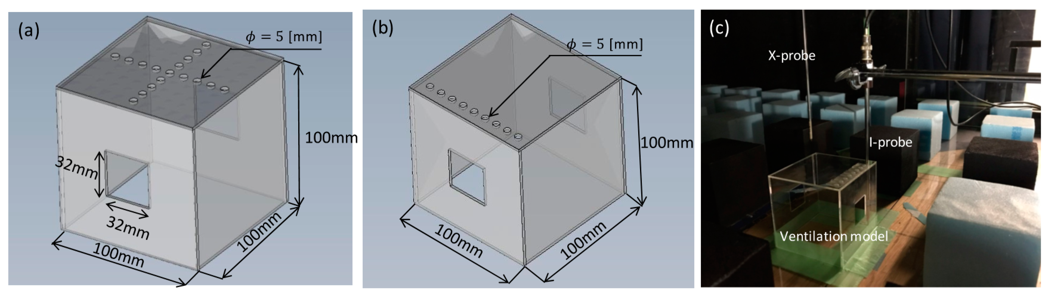
2.1. Experimental Setup

This experiment was carried out using the circulating boundary-layer wind tunnel at the Department of Environmental Energy Engineering of Kyushu University. The wind tunnel, which was 19.5 m long, had a test section of 8.0 m in length, 1.0 m in height, and 1.5 m in width. In order to fully develop the turbulent boundary layer, a dimensional rough surface made up of cube models, each with a side of 100 mm (denoted as H hereafter), was created. The cube models, which formed a building coverage ratio of 25%, were arranged in 23 rows (main stream direction) by 7 rows (spanwise direction). Figure 1 shows a schematic of the wind-tunnel test section, illustrating the cube array. The figure also indicates the position of the target-cube model which is at the 16th row; in the test-section span, the target-cube model was at the center.
The target cube was a hollow model with two openings arranged in block arrays as shown in Figure 2. The target model was made of acrylic with a thickness of 2 mm. Each opening, located at the center of the cube wall, had a size of about 10% (31.6 mm × 31.6 mm) of the wall area as shown in Figure 2c,d. Two types of cube arrays were used, i.e., a square arrangement (SQ, Figure 2a), in which the models were arranged in the same row when viewed from the main stream direction, and a staggered arrangement (ST, Figure 2b), in which the models were arranged in a staggered pattern. There were two opening positions: Streamwise (STR) and lateral (LAT), as shown in Figure 2c,d. By combining these conditions, we adopted four conditions, namely ST-STR, SQ-STR, ST-LAT and SQ-LAT.
In addition, holes with a diameter of 5 mm were provided on the upper surface, as shown in Figure 3a,b, according to the internal-measurement cross section. In this study, the openings of the target model were subject to two orientations, perpendicular and parallel, with respect to the main stream, as shown in Figure 3. The main stream direction, span direction, and vertical direction are defined as x, y, and z, respectively. Figure 3c shows the installation of the block arrays, target block, and hot-wire anemometers for SQ-STR conditions.

2.2. Measurement

In this experiment, the air-flow field around the target model and the wind speed therein were measured simultaneously using two hot-wire anemometers, as shown in Figure 4. An upstream X-type probe (KANOMAX, 0249R-T5) was placed in the canopy layer outside the model, and the wind speeds of the two components (ux, wx) were measured. An I-type probe (KANOMAX, 0251R-T5) was installed inside the model, and the in-plane wind speed perpendicular to the hot wire and the scalar wind speed (v1), affected by the wind-velocity component along the hot wire, were measured as the internal flow velocity.
When the measurement was performed, the position of the upstream X-type probe was fixed, while the I-type probe was inserted through the measurement hole before traversing from z = 5 mm to z = 95 mm at 3 mm intervals. The outer diameter of the probe support was 4.6 mm, while the inner diameter of the measuring hole was 5 mm. The inflow and outflow of air from the measuring hole was suppressed as much as possible. The upstream X-type probe was installed at a height of 1H at five measurement points under the perpendicular opening condition and three under the parallel opening condition; these points functioned as reference points that were expected to have a large effect on air introduction. The measurement time was 30 s, and the measurement frequency was 1000 Hz. Ikegaya et al. [17] showed that the maximum range of the bias errors for the mean wind speed and standard deviations were less than 0.2% and 2%, respectively, using the same type of hot-wire anemometry. Holes that were not used during the measurement were sealed off using tape on the inside and outside of the target model. The wind speeds measured by the I-type and X-type probes are referred to as v I and ( u x ,   w x ), respectively. The fluctuation part of v I and ( u x ,   w x ) are denoted as v I , u’x, and w’x, respectively.

3. Results

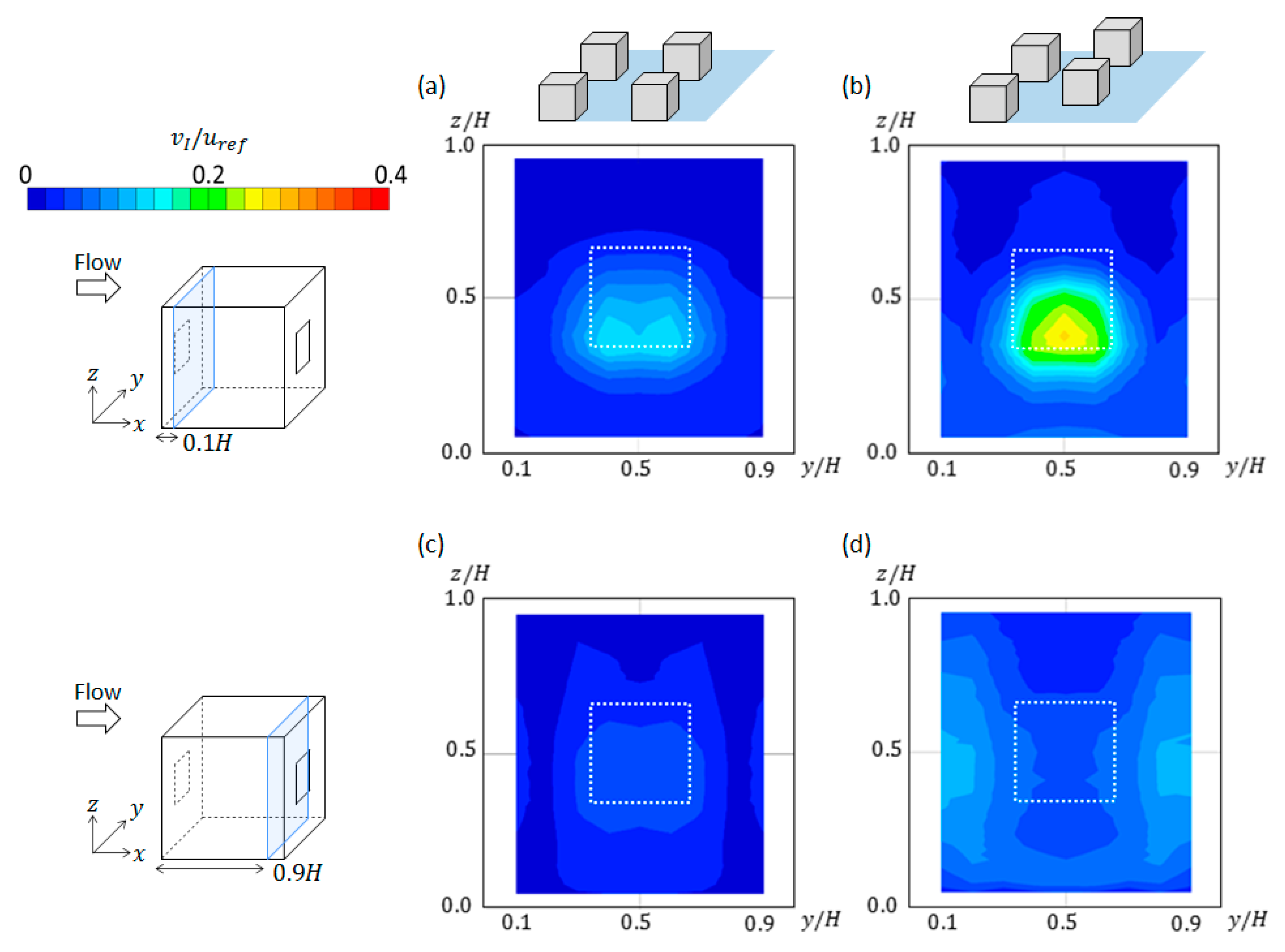
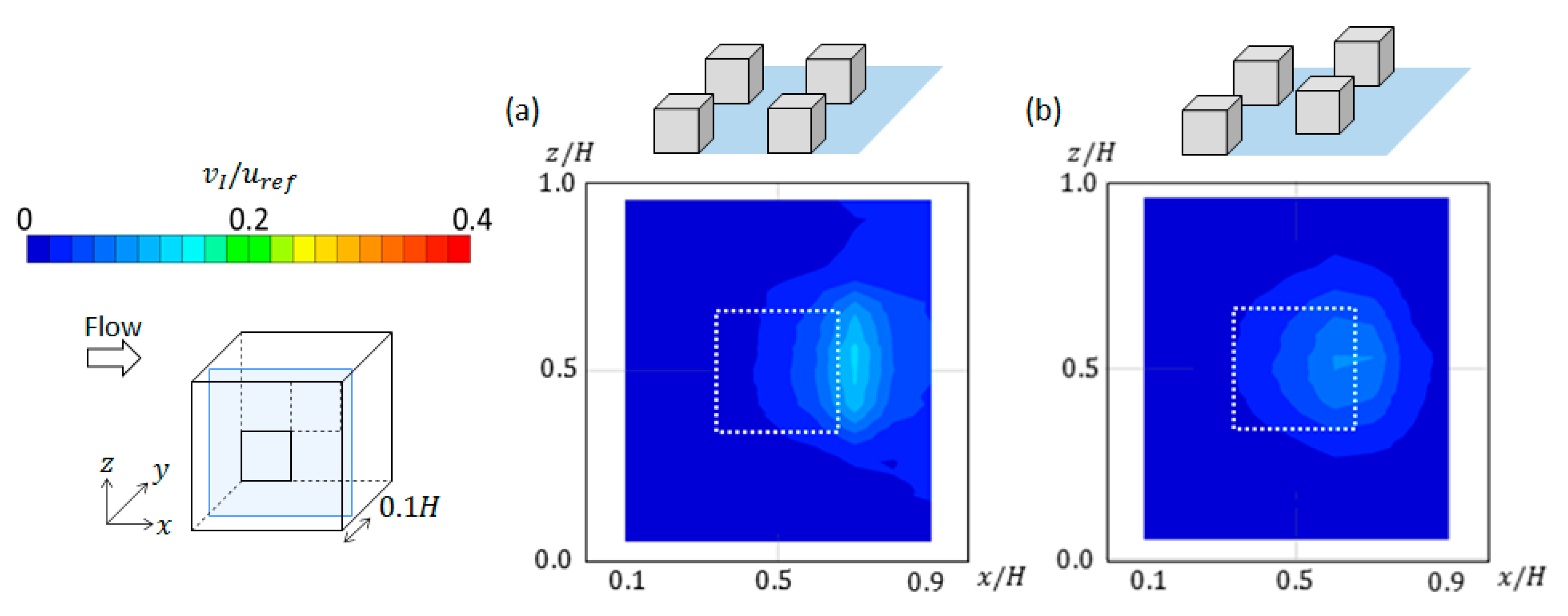
3.1. Mean Flow Field

To analyze the introduction of air into the target model, the mean flow field in the target model was extracted from the wind-tunnel data and presented in diagrams. Figure 4 shows the distribution of mean wind speed, v1, in the y-z cross section (x/H = 0.1) under ST-STR and SQ-STR. The dotted line in the figure indicates the opening position on the windward surface. As shown in Figure 4a,b, it can be confirmed that the mean wind speed was relatively high at the bottom of the windward opening. This is because the airflow was introduced from the upper part into the canopy due to the influence of the neighboring model. Such observations were consistent with previous studies [5,6,15].
Comparing the two arrays, the mean wind speed near the opening was more than 0.2 for the ST arrangement, whereas that in the SQ arrangement was less than 0.1. The ST cube models were arranged alternately, creating a larger upwind region between two consecutive cube models in the streamwise direction. Unlike in the SQ array, the target model in the ST array experienced less blockage for the mean flow path to reach its windward wall, as shown in previous studies [18,19,20]. This observation is further supported by the findings of Ikegaya et al. [16], who showed that there was a higher instantaneous streamwise velocity at an indoor point near the windward opening of a target cube in the ST array compared to the SQ array. The findings in the aforementioned previous studies are consistent with our observation of the higher mean wind speed near the windward opening in the target ST cube model.
In addition, Figure 4c,d display the mean wind-speed distributions near the leeward openings (x/H = 0.9) of the target cubes in the SQ and ST arrays. The figures shown further demonstrate that the mean wind speed of the flow entering the windward opening affects the mean wind distribution near the leeward opening [16]. Additionally, the mean wind flow in the lee of the target cube, characterized by a reverse flow [18], may also affect the mean wind-speed distribution inside the leeward opening. A previous study by Kim et al. [21] is in agreement with the lower mean wind speeds observed in the present study near the leeward opening. Moreover, the skimming-flow effect typically observed in the roughness arrays with coverage ratios of equal to or more than 25% [22,23] may also lead to this observation.
Figure 5 shows the in-plane (y/H = 0.1) mean wind-speed distribution of ST-LAT and SQ-LT. The figure demonstrates that the wind speed slightly increased in the main stream direction near the opening in both arrangements. This is likely because of the unobstructed mean flow path in the street area between the rows of the outdoor models [18,19]. The large difference between pressures outside and inside the target cube increases the probability of air introduction through the parallel opening in the SQ target cube. In fact, this causes the mean wind speed in the SQ array to be higher than that in the ST array. In the ST array, this is not quite significant, since the mean flow path leading to the opening of the target cube is obstructed, causing the wind flow to lose momentum and reduce its speed as it approaches the parallel opening.
From the presented findings, it was confirmed that the difference in the outdoor model arrangement conditions and the opening position has a significant influence on the average opening wind speed.

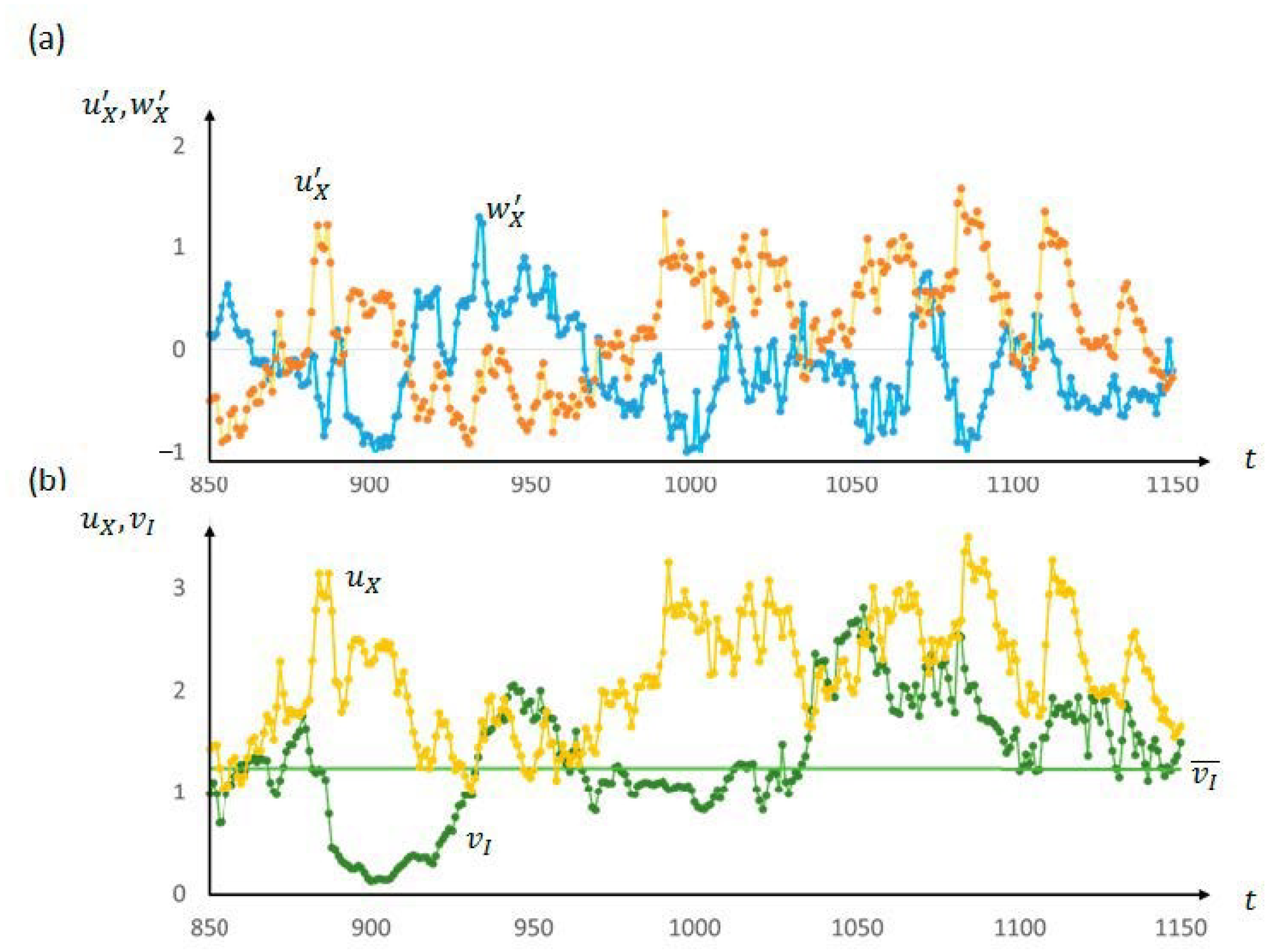
3.2. Temporal Correlation of Indoor and Outdoor Wind Speeds

To illustrate the characteristics of the temporal change in indoor and outdoor wind speeds, Figure 6 shows the time-series fluctuations of the outdoor velocity and indoor wind speed near the perpendicular opening of the target cube in the ST-STR. In Figure 6a, the time-series fluctuations of u’x and w’x, which represent the velocity-variation components in the x-direction measured by the X-type probe, are rather significant. Both components fluctuate between negative and positive values, resulting in large variations which occur continuously near the windward opening, as shown by Ikegaya et al. [16]. On the other hand, Figure 6b shows the time-series fluctuations of ux and v1, which represent the mean wind-velocity fluctuation components measured by the I-type probe. Large fluctuations of both velocity components also occurred continuously due to the surrounding interference, which caused turbulent flow structures to form in street canyons [18]. Since the outdoor Reynolds stress is usually negative, indicating that the downward momentum transport occurred, it is possible to observe the negative correlation between u x and w x in Figure 6a. Interestingly, such fluctuations of u x also caused temporal variations in the indoor velocity, v I , with a slight temporal delay of approximately 50 ms. In summary, the presented figures indicate that indoor wind speed becomes turbulent because of the turbulent outdoor air flows generated by the surrounding buildings.
To quantitatively evaluate the correlation between the outdoor air flow and the internal flow of the model, the two-point correlation coefficient, RuXvI(∆t) inside and outside the model, considering the delay time of Δt, was calculated by the following equation:
R u X v I ( t ) = u X ( t ) v I ( x , y , z , t + t ) ¯ σ u X ( t ) σ v I ( z , t + t )
where u’X is the velocity-variation component in the x-direction measured by the X-type probe, vI’(x, y, z, t) is the mean wind-velocity fluctuation component measured by the I-type probe inside the measurement target point defined by coordinates (x, y, z), σ(uX) is the standard deviation of uX, and σ(vI) is the standard deviation of vI. Figure 7, Figure 8, Figure 9 and Figure 10 show the two-point correlation-coefficient distribution under each opening condition.
Figure 7 shows the perpendicular opening in the x-z plane (y/H = 0.5) in the ST-STR arrangement and the reference point (i.e., the location where the X-type probe was placed) with the coordinates x = −0.5 H and y = −0.5 H from the measurement target. In Figure 7a, the largest positive correlation can be seen in the slightly downward position from the windward opening. In the upper region where z/H ≥ 0.5, the correlation coefficient was extremely small, i.e., 0.1 or less. In Figure 7b, the correlation-coefficient distribution at the delay time of Δt = 50 ms shows a strong positive correlation mainly in the region located near the windward opening, where z/H ≤ 0.5 and x/H ≤ 0.5. As shown in Figure 7c, when the delay time was Δt = 100 ms, the positive correlation near the windward opening was weakened, and the correlation near the model floor was strengthened. In addition, a region with an inverse correlation could be seen near the upper part of the windward opening. The time change of the above correlation-coefficient distribution was due to a strong downward flow that entered the model through the windward opening.
In Figure 7d–f, the correlation-coefficient distribution is shown for the mean velocity variation in the z-direction. At Δt = 0, a strong negative correlation was observed near the windward opening and towards the leeward opening. Subsequently, the distribution of negative the correlation coefficient moved downward at Δt = 50 ms, indicating a strong downward flow in the target model due to the introduction of air flow from the outside. Then, the lower distribution of the correlation coefficient was observed at Δt = 100 ms. This is consistent with the distribution of the correlation coefficient for the velocity component in the x-direction.
Figure 8 and Figure 9 show the correlation-coefficient distributions in the y-z cross section near the windward opening for ST-STR and SQ-STR, respectively. The reference position was x/H = −0.5 and y/H = 1.5, respectively, as shown in Figure 8. The measurement on the y-z plane was at x/H = 0.1. The basic correlation trends were similar in both ST and SQ arrays. However, the correlation coefficient of the SQ array was larger than that of the ST array due to the unsheltered air-flow introduction from the outside in the SQ array. The street region between two consecutive rows of cubes in the SQ array was typically characterized by high wind velocity [18], and this induced the introduction of air into the target model. In the ST array, the reference point, which was outside the target model, lay in the lee of a neighboring model; the reverse flow in this region did not lead to a significant introduction of air into the target model. Despite the difference in terms of the degree of influence between the two arrays, this observation clearly illustrates the effect that the outdoor airflow has on the indoor airflow.
A similar observation may be made in Figure 9 for the correlation coefficient distribution near the opening parallel to the wind direction. The reference position was at x/H = 0 and y/H = 1.5, as shown in Figure 9. The measurement plane was at x/H = 0.9. The distribution was consistent with the results of mean flow near the parallel opening shown in Figure 5; the target model in the SQ array was recorded with the higher mean wind speed, corresponding to the higher positive correlation near its opening. This indicated a strong correlation between the outdoor and indoor flows in the SQ array, which was not observed in the target model of the ST array. The flow path was disrupted in the ST array due to the surrounding building arrangement. Consequently, the correlation between the outdoor and indoor flows was lower.
Finally, Figure 10 shows the correlation-coefficient distribution in the y-z plane (y/H = 0.1). The reference point was at x/H = 0 and y/H = −1.5. Here, the results of ∆t = 20 ms, showing the correlation-coefficient distributions, are shown for both the ST and SQ arrays. In the ST arrangement, the correlation coefficient was zero, suggesting a negligible impact of the outdoor air flow on the air introduction into the target model. This might have been due to the location of the reference point and the opening of the target model which were downstream of nearby models. Such locations were sheltered from the undisturbed flow path. On the other hand, in the SQ arrangement, when the air flow in the street area flowed into the canyon, air was introduced into the target model. This resulted in a stronger inverse correlation in y/H ≥ 0.5 and a strong positive correlation in y/H ≤ 0.5.

4. Conclusions

A series of wind-tunnel experiments were conducted using hot-wire anemometry for the turbulent urban-canopy flow fields generated by ST and SQ arrays. A target ventilation building with several openings was immersed within the block arrays. The outdoor and indoor wind speeds were measured simultaneously. The results indicated that the wind speed near the windward openings on the streamwise faces showed 0.3 to the reference wind speed, whereas those on the lateral faces were less than 0.1. In contrast, the indoor wind speeds were higher than 0.1 in the target model in the SQ array for the openings on the lateral faces to the wind-flow direction. These results quantitatively clarify that both the arrangements of surrounding buildings and the opening positions have a significant influence on the introduction of air into the target building. This implies that the indoor ventilation rate is significantly affected by the surrounding conditions due to complex, turbulent urban-canopy flows.
In addition, the correlation between the outdoor and indoor air flows was quantified by determining the two-point correlation coefficients. The highest correlations were obtained for both opening conditions with a certain temporal delay. This result indicates that indoor air flows become turbulent because of the turbulent flows generated by the surrounding outdoor buildings; however, slight temporal delays may occur. The correlation-coefficient distribution was influenced by the surrounding building arrangement, whereby the square array promoted more air introduction into the target model than in the staggered array with the same temporal delay. On the whole, the fundamental turbulent characteristics of indoor and outdoor air flows obtained in this study are essential for predicting ventilation-flow rates due to turbulent air flows, and are applicable for sheltered buildings.

Author Contributions

Conceptualization, N.I. and A.F.M.; methodology, R.H.; investigation, R.H.; writing—original draft preparation, R.H., A.F.M., N.I. and S.A.Z.; writing—review and editing, N.I. and A.F.M.; visualization, R.H.; funding acquisition, S.A.Z. All authors have read and agreed to the published version of the manuscript.

Funding

This work was partially supported by the Ministry of Education (MOE) through the Fundamental Research Grant Scheme [FRGS/1/2019/TK07/UTM/02/5], Fellow Research Grant [Vot 00P01] under Universiti Teknologi Malaysia, and Takasago Engineering Ltd. Grant [Vot 4B424].

Institutional Review Board Statement

Not applicable.

Informed Consent Statement

Not applicable.

Data Availability Statement

Not applicable.

Acknowledgments

The authors would like to acknowledge Aya Hagishima of Kyushu University for her valuable suggestion for conducting this work.

Conflicts of Interest

The authors declare no conflict of interest.

References

  1. Seifert, J.; Li, Y.; Axley, J.; Rösler, M. Calculation of wind-driven cross ventilation in buildings with large openings. J. Wind Eng. Ind. Aerodyn. 2006, 94, 925–947. [Google Scholar] [CrossRef]
  2. Asfour, O.S.; Gadi, M.B. A comparison between CFD and Network models for predicting wind-driven ventilation in buildings. Build. Environ. 2007, 42, 4079–4085. [Google Scholar] [CrossRef]
  3. Jiang, Y.; Alexander, D.; Jenkins, H.; Arthur, R.; Chen, Q. Natural ventilation in buildings: Measurement in a wind tunnel and numerical simulation with large-eddy simulation. J. Wind Eng. Ind. Aerodyn. 2003, 91, 331–353. [Google Scholar] [CrossRef]
  4. Hiyama, K.; Kato, S.; Takahashi, T.; Kono, R. Study on effect of opening area ratio and relative opening location on air flow characteristics in cross-ventilation models. J. Environ. Eng. (Trans. AIJ) 2005, 70, 21–27. [Google Scholar] [CrossRef]
  5. Kasim, N.F.M.; Zaki, S.A.; Ali, M.S.M.; Ikegaya, N.; Razak, A.A. Computational study on the influence of different opening position on wind-induced natural ventilation in urban building of cubical array. Procedia Eng. 2016, 169, 256–263. [Google Scholar] [CrossRef]
  6. Zaki, S.A.; Kasim, N.F.M.; Ikegaya, N.; Hagishima, A.; Ali, M.S.M. Numerical simulation on wind-driven cross ventilation in square arrays of urban buildings with different opening positions. J. Adv. Res. Fluid Mech. Therm. Sci. 2018, 49, 101–114. [Google Scholar]
  7. Ohba, M.; Irie, K.; Kurabuchi, T. Study on airflow characteristics inside and outside a cross-ventilation model, and ventilation flow rates using wind tunnel experiments. J. Wind Eng. Ind. Aerodyn. 2001, 89, 1513–1524. [Google Scholar] [CrossRef]
  8. Kotani, H.; Sagara, K.; Yamanaka, T. Airflow field analysis around the building during ventilation by PIV. J. Vis. Inf. Soc. 2009, 29, 18–24. [Google Scholar]
  9. Karava, P.; Stathopoulos, T.; Athienitis, A.K. Airflow assessment in cross-ventilated buildings with operable façade elements. Build. Environ. 2011, 46, 266–279. [Google Scholar] [CrossRef]
  10. Arinami, Y.; Akabayashi, S.; Takano, Y.; Tominaga, Y.; Sakaguchi, A. Visualization and measurements for fluctuating cross ventilation airflow in simple house model using large-size boundary layer wind tunnel: Study on PIV measurement and analysis for room air flow distribution Part 2. J. Environ. Eng. (Trans. AIJ) 2015, 80, 127–137. [Google Scholar] [CrossRef] [Green Version]
  11. Bangalee, M.Z.I.; Miau, J.J.; Lin, S.Y.; Yang, J.H. Flow visualization, PIV measurement and CFD calculation for fluid-driven natural cross-ventilation in a scale model. Energy Build. 2013, 66, 306–314. [Google Scholar] [CrossRef]
  12. Shirzadi, M.; Mirzaei, P.A.; Naghashzadegan, M. Development of an adaptive discharge coefficient to improve the accuracy of cross-ventilation airflow calculation in building energy simulation tools. Build. Environ. 2018, 127, 277–290. [Google Scholar] [CrossRef]
  13. Tominaga, Y.; Blocken, B. Wind tunnel experiments on cross-ventilation flow of a generic building with contaminant dispersion in unsheltered and sheltered conditions. Build. Environ. 2015, 92, 452–461. [Google Scholar] [CrossRef] [Green Version]
  14. Hasegawa, Z. Winds of Buildings with Openings in the Urban Turbulent Boundary Layer: PIV Measurement. Master’s Thesis, Kyushu University, Fukuoka, Japan, 2018. [Google Scholar]
  15. Van Hooff, T.; Blocken, B.; Tominaga, Y. On the accuracy of CFD simulations of cross-ventilation flows for a generic isolated building: Comparison of RANS, LES and experiments. Build. Environ. 2017, 114, 148–165. [Google Scholar] [CrossRef]
  16. Ikegaya, N.; Hasegawa, S.; Hagishima, A. Time-resolved particle image velocimetry for cross-ventilation flow of generic block sheltered by urban-like block arrays. Build. Environ. 2019, 147, 132–145. [Google Scholar] [CrossRef]
  17. Ikegaya, N.; Morishige, S.; Matsukura, Y.; Onishi, N.; Hagishima, A. Experimental study on the interaction between turbulent boundary layer and wake behind various types of two-dimensional cylinders. J. Wind Eng. Ind. Aerodyn. 2020, 204, 104250. [Google Scholar] [CrossRef]
  18. Coceal, O.; Thomas, T.G.; Castro, I.P.; Belcher, S.E. Mean flow and turbulence statistics over groups of urban-like cubical ob-stacles. Bound. -Layer Meteorol. 2006, 121, 491–519. [Google Scholar] [CrossRef]
  19. Lin, M.; Hang, J.; Li, Y.; Luo, Z.; Sandberg, M. Quantitative ventilation assessments of idealized urban canopy layers with various urban layouts and the same building packing density. Build. Environ. 2014, 79, 152–167. [Google Scholar] [CrossRef]
  20. Razak, A.A.; Hagishima, A.; Ikegaya, N.; Tanimoto, J. Analysis of airflow over building arrays for assessment of urban wind environment. Build. Environ. 2013, 59, 56–65. [Google Scholar] [CrossRef]
  21. Kim, Y.C.; Tamura, Y.; Yoon, S.-W. Proximity effect on low-rise building surrounded by similar-sized buildings. J. Wind Eng. Ind. Aerodyn. 2015, 146, 150–162. [Google Scholar] [CrossRef]
  22. Zaki, S.A.; Hagishima, A.; Tanimoto, J. Experimental study of wind-induced ventilation in urban building of cube arrays with various layouts. J. Wind Eng. Ind. Aerodyn. 2012, 103, 31–40. [Google Scholar] [CrossRef]
  23. Ikegaya, N.; Hirose, C.; Hagishima, A.; Tanimoto, J. Effect of turbulent flow on wall pressure coefficients of block arrays within urban boundary layer. Build. Environ. 2016, 100, 28–39. [Google Scholar] [CrossRef]
Figure 1. Schematics of the wind-tunnel device, where 15 rows of cubical blocks were arranged upstream of the target ventilation model.
Sustainability 13 00586 g001
Figure 2. Schematics of block arrangement and opening positions. (a) Square array (SQ), (b) staggered array (ST) (c) Streamwise (STR) openings, and (d) Lateral (LAT) openings. l = 32 mm and H = 100 mm represent the opening length and the block height, respectively.
Sustainability 13 00586 g002
Figure 3. Measurement locations of ventilation model for (a) indoor wind speed and (b) near-opening wind speed. (c) Photograph showing installations of an X-probe to measure outdoor velocity and I-probe to measure indoor wind speed.
Sustainability 13 00586 g003
Figure 4. Mean wind-speed distribution in the y-z cross section near the opening for streamwise openings at (a,b) x / H   =   0.1 and (c,d) x / H = 0.9 , respectively. (a,c) ST-STR, and (b,d) SQ-STR. The white, dashed lines indicate the opening location.
Sustainability 13 00586 g004
Figure 5. Mean wind-speed distribution in the x-z cross section near the opening at y / H   =   0 .1 for (a) SQ-LAT, and (b) ST-LAT. The white, dashed lines indicate the opening location.
Sustainability 13 00586 g005
Figure 6. Time series of (a) outdoor velocity and (b) indoor wind speed for ST-STR.
Sustainability 13 00586 g006
Figure 7. Distributions of the two-point correlation coefficient between indoor and outdoor wind speeds within the vertical cross section at y / H = 0.5 for ST-STR. (ac) R u X v I and (df) R w X v I . Time delays in distributions are (a,d) Δ t = 0 , (b,e) Δ t = 50 ms, and (c,f) Δ t = 100 ms, respectively.
Sustainability 13 00586 g007
Figure 8. Distributions of the two-point correlation coefficient between indoor and outdoor wind speeds within the vertical cross section at x / H = 0.5 for (a) ST-STR and (b) SQ-STR. The time delay for the distributions shown is Δ t = 20 ms.
Sustainability 13 00586 g008
Figure 9. Distributions of the two-point correlation coefficient between indoor and outdoor wind speeds within the vertical cross section at y / H = 0.9 for (a) ST-LAT and (b) SQ-LAT. The time delay for the distributions shown is Δ t = 20 ms.
Sustainability 13 00586 g009
Figure 10. Distributions of two-point correlation coefficient between indoor and outdoor wind speeds within the vertical cross section at y / H   =   0.1 for (a) ST-LAT and (b) SQ-LAT. The time delay for the distributions shown is Δ t = 20 ms.
Sustainability 13 00586 g010
Publisher’s Note: MDPI stays neutral with regard to jurisdictional claims in published maps and institutional affiliations.

