Abstract
Estimating sediment flow rate from a drainage area plays an essential role in better watershed planning and management. In this study, the validity of simple and wavelet-coupled Artificial Intelligence (AI) models was analyzed for daily Suspended Sediment (SSC) estimation of highly dynamic Koyna River basin of India. Simple AI models such as the Artificial Neural Network (ANN) and Adaptive Neuro-Fuzzy Inference System (ANFIS) were developed by supplying the original time series data as an input without pre-processing through a Wavelet (W) transform. The hybrid wavelet-coupled W-ANN and W-ANFIS models were developed by supplying the decomposed time series sub-signals using Discrete Wavelet Transform (DWT). In total, three mother wavelets, namely Haar, Daubechies, and Coiflets were employed to decompose original time series data into different multi-frequency sub-signals at an appropriate decomposition level. Quantitative and qualitative performance evaluation criteria were used to select the best model for daily SSC estimation. The reliability of the developed models was also assessed using uncertainty analysis. Finally, it was revealed that the data pre-processing using wavelet transform improves the model’s predictive efficiency and reliability significantly. In this study, it was observed that the performance of the Coiflet wavelet-coupled ANFIS model is superior to other models and can be applied for daily SSC estimation of the highly dynamic rivers. As per sensitivity analysis, previous one-day SSC (St-1) is the most crucial input variable for daily SSC estimation of the Koyna River basin.
1. Introduction
To prevent soil degradation and improve the water quality, the soil and water management treatments must be carried out at the watershed level. Sediment loss measurement is crucial to assess soil and water conservation treatments on sediment flow through the river [1,2,3]. Sediment transport information is essential for designing and planning soil and water conservation structures on the river. The sediment movement’s magnitude depends on rainfall volume and intensity, Land Use/Land Cover (LULC), topography, and soil physical properties [4]. Sediment concentration flow prediction is important because the accumulation of sediments reduces the reservoir capacity. It also reduces the productivity of such land over which sedimentation takes place. Sedimentation is responsible for increasing the flood hazard due to sediment mass trapping over the river bed [2,5].
Accumulated sediment also blocks the entrance of the intake structure. It also reduces the flow capacity and increases the maintenance and repair cost of irrigation and drainage channels. Increased sediment concentration reduces the available dissolved oxygen in water; hence it is responsible to retard water life [6]. Increased sediment concentration is responsible for increasing the domestic and drinking water purification cost. Higher sediment flow also carries contaminants developed over upstream areas due to point and non-point pollution sources and increases environmental pollution. Sediment flow forms visual pollution, and hence it reduces the recreational potential of wetlands and lakes. It also reduces fish eggs proliferation by accumulating over the surroundings [6,7]. Sediment load information is essential for the design of reservoirs and dams, stable channels, the design of lakes and estuaries, the reduction of sediment and pollutants flow in rivers, environmental impact assessment, and the wildlife protection of fish habitats [4].
Suspended sediment load measurements are carried out by taking samples along the river section using different samplers. Such samplers truly represent the flowing sediment concentration at a given measuring point of river cross-section. It is still very time-consuming, expensive, and frequent sampling cannot be easily conducted [8,9]. Another method of suspended sediment load measurement is empirical and semi-empirical equations that depend on laboratory experiments conducted under uniform flow conditions with uniform bed material [1]. Still, it is contradictory to real practical conditions [7]. The existing empirical equations and theories available in the literature for sediment load computation are only approximate values because of the complex interaction between sediment transport and water movement. It is challenging to describe sediment flow mathematically because of such a complex relationship between discharge and sediment flow. Different empirical equations provide different results with significant errors [7,10]. The relationship between suspended sediment and discharge is significant in the estimation of sediment load. In the past, many studies have been conducted for the sediment modeling process.
Generally, mathematical models require many data with a long response time, which is rarely available [11]. The detailed information of the watershed’s physical properties must be known [12]. The traditional methods are limitedly used and not preferable because of non-linear relationships among hydrological variables and dependence on many hydrological field data [13]. Hence, it is quite a tricky task to forecast a non-stationary time series by using statistical models. However, it is essential to select alternative models to disseminate non-stationary and non-linearity in the time series data. The Artificial Intelligence (AI) technique has an advantage over traditional methods. It can perform well with a large amount of noisy data resulting from the dynamic and non-linear system where the system’s fundamental physical relationships are unknown [14,15,16,17]. AI techniques can solve the complex problems of different hydrologic processes [18]. A black box model such as an Artificial Neural Network (ANN) does not need watershed physical characteristics to transform inputs into an output and to recognize any hydrologic process [8,19]. AI-based data-driven models such as ANN do not need site-specific information that is rarely available but instead focuses on forming the relationship between input and output variables [20,21,22]. The modeling of different hydrological processes using ANN is the latest technique [23]. It considers both linearity and non-linearity concepts for model construction. It can perform satisfactorily for the memoryless or dynamic input–output system.
Therefore, ANNs have been used in most of the application areas. Some of the application areas are water resource and hydrology, including modeling of drought, rainfall-runoff, water quality, runoff-sediment, precipitation forecasting, climate change impacts on streamflow, sediment transport process, and groundwater quality and groundwater level forecasting, water level forecasting in aquifers and lakes [7,24,25,26] •ANN is a modeling tool capable of identifying high complexity present in input-output data, which operates by considering previously recorded input-output data [12] •ANN modeling is crucial for predicting suspended sediment concentration in the river flow [27] • ANN is considered as a lumped parameter model to simulate rainfall, runoff, and sediment • ANN undergoes strong generalization ability; once the ANN architecture is adequately trained, ANN can give accurate results even for those that have never been seen before [28]. •Many researchers have recently applied the ANN model for rainfall–runoff and runoff–sediment modeling [4,19,20,24,28].
The time-series data used for rainfall–runoff–sediment modeling usually contains uncertainties. In such a case, the fuzzy theory can be adapted to model these uncertainties to solve real-world problems. Adaptive Neuro-Fuzzy Inference System (ANFIS) can be made by combining ANN and fuzzy logic and subsequently receiving benefits from both [22,26]. The ANN model must perform a trial-and-error process to generate the optimal network architecture. Still, the ANFIS model is free from such a tedious procedure. The ANFIS is a multilayer self-organize network structure that adapts the fuzzy system’s parameters to predict the system output. However, the fuzzy logic approach’s main problem is that no systematic procedure is available to design a fuzzy controller [12]. The ANFIS technique has recently been applied successfully for rainfall–runoff–sediment modeling [7,21,23]. Generally, Fourier transform requires static data for investigation purposes, but signals of hydrological time series are highly non-stationary. The difficulty with Fourier transforms during non-stationary hydrologic modeling is that it only considers the central time-series’ frequency feature. It is suitable only for static time series [29].
To overcome this weakness, a wavelet transform can be used. Wavelet transform comes into effect while modeling with non-stationary data. It can produce different series which identify possible trends, seasonal variations, and internal correlation among different components [20]. Wavelet analysis consists of the shifting and scaling of the original (mother) wavelet. Wavelet transform improves the model performance because it simultaneously considers both temporal and spectral information available within the signal; this feature overcomes the Fourier analysis’s fundamental limitation. The Fourier spectrum provides only globally averaged information [26]. Wavelet transform decomposes primary time series data into different sub-components without losing any information and extracting required information from historical data using few coefficients. It reveals the hidden information available in the data. It provides a more concise form of original time series data with a timescale representation of processes relationships within them [30,31]. Hence, wavelet data-driven models use these different sub-components’ data, which improves the model’s performance by capturing the required information available in the central time series hydrological data [22,32]. Different researchers recently used the wavelet transform technique for hydrological time series modeling to improve models’ performance accuracy. Grossmann and Morlet [33] introduced wavelet transform, which can reveal the different aspects of time series data such as breakdown points, trends, and discontinuities; this is the superiority of wavelet over other signal analysis techniques [31,32,34].
In a few last years, simple data-driven models, as well as the coupling of data-driven models and wavelet transform, have been applied successfully for hydrological modeling [29,35,36,37]. Accordingly, this study has been carried out with the following objectives: (a) Select the best input variables for reasonable daily SSC prediction of Koyna River basin using the Gamma test (GT). (b) Develop simple AI and hybrid wavelet-coupled AI models for daily SSC prediction of the study area. (c) Assess the reliability of the best-selected models using uncertainty analysis, and (d) analyze the sensitivity of selected input variables for daily SSC modeling using sensitivity analysis. Different AI techniques behave differently at varying climatic and topographic conditions. Hence, in this study, such a complex river basin having a highly dynamic nature was selected to assess different AI techniques’ performance. In this study, different simple AI and hybrid wavelet-coupled AI models were developed to compare their suspended sediment estimation performances. The performance of the developed models was assessed using standard model performance criteria. The novelty of this study includes the finding that the coiflet wavelet-coupled ANFIS model could be used for daily suspended sediment estimation in highly dynamic rivers like the Koyna River basin.
2. Materials and Methods
2.1. Study Area and Data Collection
The Koyna River (a tributary of Krishna River) originates at Mahabaleshwar in the Satara district of Maharashtra, India. The Konya River flows North to South from its origin for about 65 km and then flows for about 56 km eastward to meet the Krishna River. Before taking an eastward turn, it is dammed at Koynanagar, called Koyna dam. The study area lies between 17°7′55″ N to 17°57′50″ N latitude and 73°33′15″ E to 74°11′10″ E longitude, as shown in Figure 1a.
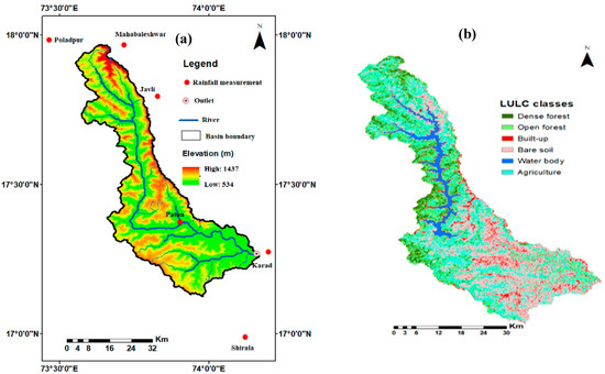
Figure 1.
(a) The geographical location and the gauging stations (b) land use/land cover of the Koyna River basin.
The Koyna River basin has a geographical area of 1917 km2 on the Deccan plateau. The study area comes under the survey of India toposheets 47G/9, 47G/11, 47G/11, 47G/13, 47G/14, 47G/15, 47G/16, 47K/13, and 47K/14. The study area comes under varying climatic and topographic conditions. The annual rainfall at the upstream part of the basin is 5000 mm, reducing to 866 mm downstream. About 88% rainfall occurs in the monsoon (1 June to 30 September) season. In this study, the mean areal rainfall of the study area was determined using the Thiessen polygon method in ArcGIS 10.2 software. The study area comes under a subtropical climate. The winter season starts in October and extends up to January, while the summer season extends from February to May. The daily mean monthly maximum temperature varies between 31 °C to 37 °C, while the daily mean monthly minimum temperature varies between 10 °C to 14 °C. Agriculture is the primary source of income for people who lives in the River basin. The soil at the upstream part of the basin is light laterite, while the central and downstream area is under black cotton soil. The elevation in the basin varies between 534 m to 1437 m above the mean sea level. The dominant part of the basin is under the steep sloping condition with varying topography and prone to soil loss. The entire basin area is covered by agriculture (717.13 km2), bare soil (491.69 km2), open forest (342.60 km2), dense forest (159.84 km2), built-up land (120.20 km2), and water body (85.68 km2), as shown in Figure 1b which was prepared using ArcGIS 10.2 software in this study runoff and sediment measurements were conducted at the basin’s outlet, situated at Warunji village in the Satara district.
The monsoon season’s daily rainfall data from 1999 to 2005 (7 years) were collected from the agricultural department of Maharashtra state, India. The daily runoff and suspended sediment concentration (SSC) data of monsoon season for the same duration reported for rainfall were collected from India’s central water commission (CWC). Out of the total data, the first 70% data were used for training. The remaining 30% of the data were used for testing the developed models.
2.2. ANN
ANN is inspired by the biological (brain) neuron system. Each neuron receives processes and sends the signal to make functional relationships between future and past events [38]. The most common structure of ANN is shown in Figure 2.
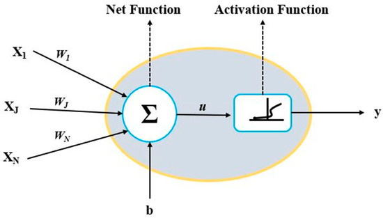
Figure 2.
The basic structure of ANN.
ANN consists of the input layer, one or more hidden layers, and the output layer. In the neural network, each neuron (node) has input variables and output variables. A neuron determines the output variable’s value after applying the net and activation (transfer) function on input variables. The net function (u) is determined by adding the product of input variables (xi) with their corresponding connection weights (Wi) plus the bias or threshold value (b) of a neuron. Usually, the net function is in the linear form given as:
where xi is an input variable, Wi is the connection weight from the ith neuron in the input layer, and b is the bias/threshold value of the neuron [39]. The net function (u) at a hidden node is transformed into output (y) using a non-linear activation function. More details of ANN were added in the Appendix A.
2.3. ANFIS
The Fuzzy Inference System (FIS) is a popular computing framework that depends on fuzzy set theory. The building blocks of FIS are the fuzzy operators, fuzzy sets, and the knowledge base. It allows extracting fuzzy rules from expert knowledge or numerical data and constructs a rule base adaptively. Moreover, it can adapt to the complicated conversion of human intelligence to fuzzy systems. Fuzzy theory can be adapted to model the uncertainties to solve real-world problems. For prediction purposes, the ANFIS model is better than the ANN model in peak flow prediction accuracy, prediction error, and computational error [26]. ANFIS is functionally equivalent to FIS; it is a multilayer feed-forward network that uses ANN learning algorithms and fuzzy reasoning to characterize an input space to an output space, powerful in modeling numerous time series processes.
ANFIS is a universal approximator because it has set-off If-Then rules that have the learning potential to approximate a non-linear system. It can approximate any real continuous function. ANFIS structure consists of many nodes connected through directional links with each other. Each node has to perform a specific function with adjustable or fixed parameters [40]. For first-order Takagi-Sugeno-Kang (TSK) FIS with two inputs (x and y) and one output (f), two typical rules can be expressed as:
where Ai and Bi are Membership Functions (MFs) for input x and y, respectively. Simultaneously, pi, qi, and ri are the design (consequent) parameters estimated during the training process. The TSK model’s fuzzy reasoning mechanism derives an output (f) with inputs (x and y). General ANFIS structure with two inputs, two rules, and a single output. The functioning of the ANFIS structure (five layers) is described below. The description of the ANFIS layers functions was presented in the Appendix B.
Rule 1: If x is A1 and y is B1, then f1 = p1x + q1y + r1
Rule 2: If x is A2 and y is B2, then f2 = p2x + q2y + r2
2.4. Subtractive Clustering
Data clustering is a process that puts similar data into groups. A clustering algorithm divides the whole data into various groups. The existence of similarity within a group is more than in other groups. Clustering algorithms are mostly used for data categorization as well as data compression and model construction. When there is no clear idea to select how many clusters in a given data set, then the subtractive clustering method can be used. It is a fast, one-pass algorithm to estimate the number of clusters and cluster centers in a given data set [37]. In subtractive clustering, the number of the fuzzy rule set is equal to the number of cluster centers.
Considering n data points (x1, ….., xn), subtractive clustering assumes each data point act as a candidate for representing the cluster center. The subtractive clustering depends on data density. The density index at any point xi is expressed as:
Di represents density index, and ra is positive (ra > 0), indicating the neighborhood radius in each cluster center. So, the data point which has more neighborhood points indicates more potential to represent as cluster center. Those data points which are located outside the radius create less impact on the density index. Selection of clustering radius receives greater importance while determining the number of clusters. The high value of ra causes the minimum number of clusters and vice versa. After determining a data point with a high potential to act as a cluster center, say Xc1 is a point act as a first cluster center determined by the Dci density index. The expression recalculates the next density index for each data point Xi:
where rb is a positive constant (rb > 0), which indicates the neighborhood radius for which the most significant reduction in the density will be achieved. To prevent closely spaced cluster centers, rb is usually equal to 1.5 times of ra. After this density measurement, the next cluster center Xc2 is selected. The same process is repeated until sufficient numbers of cluster centers are achieved.
2.5. Wavelet Transform
In total, two types of wavelet transform, namely, Continuous Wavelet Transform (CWT) and Discrete Wavelet Transform (DWT), are used. The DWT can capture the non-linear and non-stationary time series’ dynamic properties using different wavelet coefficients [11]. DWT analysis is mostly preferred for forecasting water resource system problems because it needs a short computational time [30]. The discrete mother wavelet can be expressed as [26]:
where a and b are the integers that control the wavelet dilation and translation, respectively. The most commonly used value for these parameters is m0 = 2 and n0 = 1, where n0 is the location parameter. It must be greater than zero and m0 displays fined dilation step that is greater than one. The DWT scale and position are based on the power of two (dyadic scales and positions); this power of two logarithmic scalings of the translation and dilation is known as the dyadic grid arrangement. The dyadic wavelet function is defined as [41]:
For a discrete-time, series, xi, the dyadic wavelet transform becomes [26]:
Ta,b is the wavelet coefficient for the discrete wavelet with scale m = 2a and location n = 2a, b. (i = 0, 1, 2,…, L-1; and L is an integer power of 2: L = 2A).Also, the signal’s smoothed component, which represents the time series’ overall trend, is considered T. The discrete inverse transform can reconstruct the signal xi as [42]:
where T(t) is the approximate sub-signal at level A and Ta,b(t) are details sub-signals at levels a = 1, 2,..., A and time dimension of t (t = 1, 2,.., b). The wavelet coefficients, Ta,b(t) with (a = 1, 2,…, A), give the detailed sub-signals which can capture small features of interpretational value available in the time series data. The residual term T(t) indicates an approximate sub-signal, representing background information available in the time series data. An approximate sub-signal represents the general trend of the original time series signal. In contrast, a detailed sub-signal represents high-frequency components of the original time series signal [42]. Using these approximate and detail sub-signals, the characteristics of time series like jump, period, hidden period, and dependence can be identified easily [22]. When the original signal passes through low and high pass filter at each decomposition level, it gets resolved into approximate and detail sub-signals; the decomposition at each level is satisfied by the condition given as:
In this study, original rainfall, runoff, and SSC time series data were decomposed through DWT into approximate and detail sub-signals using MATLAB (R2015a) wavelet toolbox.
2.6. Mother Wavelets
Different mother wavelets are characterized by their features, such as their support region and the corresponding number of vanishing moments. In this study, for investigation purposes, Haar, Daubechies, and Coiflets mother wavelets were selected for assessing their comparative prediction performance for daily SSC prediction. Some of the most-used mother wavelets are described below.
Haar wavelet: It is the first and the most straightforward form of all other wavelets. It is discontinuous and resembles a step function. It is suitable for such time series which has sudden transitions. Nevertheless, this property may be a disadvantage of the Haar wavelet as it is not differentiable [31]. Daubechies wavelet (db): It is compactly supported (finite length) orthonormal wavelets and makes discrete wavelet transform possible. It is represented by dbN where N is the number of vanishing or zero moments. The ordinary members of this family are db2, db3, db4, db5, db6, db7, db8, db9, and db10.
Coiflets wavelet (coif): In the Coiflet wavelet, both the scaling function and wavelet function have vanishing moments. It facilitates wavelet transformation and provides an excellent approximation of polynomial function at different resolutions, increasing computational efficiency. This wavelet family has four members, namely coif1, coif2, coif3, and coif4. In this study, for investigation purposes, Haar, Daubechies (db2), and Coiflets (coif2) mother wavelets were selected to assess their comparative prediction performance for daily SSC prediction. Schematic representation of the selected mother wavelets.
2.7. Gamma Test (GT)
Hydrological processes are highly complex, dynamic, and non-linear. To select the best input combination, it needs to carry out a trial-and-error procedure. GT provides useful information to select the best input variables for constructing a reliable and smooth model. It also reduces the workload required to develop models by considering all input combinations [12]. GT is a non-parametric test. GT determines the variance of noise or the Mean Square Error (MSE) without any over-fitting. GT evaluates the non-linear correlation between two random variables like input and output pairs.
GT assumes that if two variables b and b’ are close together in the input space, their corresponding output variables c and c’ should also be close in the given output space. If the outputs are not close together, then it will indicate noise. Suppose the data set is given in the form as:
where vector b ϵ RN denotes input, corresponding scaler c ϵ R denotes output. Here, the assumption is that the input vector consists of useful information that can affect output c. The relationship among variables in the system is assumed in the form as:
where s denotes the noise. Here, it is also assumed that variance of the noise is bounded. The additional Gamma test forms were illustrated in the Appendix C.
In this study, the best input combination for daily SSC prediction was selected based on a minimum value of gamma (Γ) and Vratio. To apply the GT, win GammaTM software was used.
2.8. Data Normalization
In this study, the original time series data were normalized between 0 and 1 for practical training of the developed models. It will give equal attention to all input parameters and helps in fast convergence during training. Interpretability of models improves due to normalization [30]. Here, the normalization of supplied input data was done for eliminating their dimensions using the expression as:
where Smax and Smin are the maximum and minimum values of original time series data, n is the number of data points, and x is the original input variable’s normalized value.
2.9. Training and Testing of Developed Models
MLP based feed-forward ANN is the most commonly used in hydrology while coupling with wavelet transform [32]. In this study, feed-forward MLP based ANN models were trained and tested in MATLAB (R2015a) software. The single hidden layer with (BP) algorithm can model the input-output system’s complex and non-linear behavior [30]. Hence, in this study, three layered (one input, one hidden, and one output layer) neural network models were developed for daily SSC prediction. The most accurate, reliable, and fast BP based Levenberg-Marquardt (LM) learning rule was used to train neural network models [30,39]. The selection of the number of neurons in the hidden layer is also a difficult task. The number of neurons in the input layer is equal to the number of input variables. In contrast, the number of neurons in the output layer is the same as that of the number of output variables (only one in this study). To date, no clear guideline is available to select the optimum number of neurons in the hidden layer. However, Olyaie, et al. [11] suggested that the hidden layer neurons should be increased from (2(√n) + m) to (2n + 1) for selecting the optimal number, where n is the number of input variables and m is the number of output variables. It can solve the problem of under- and over-fitting of models. Due to under- and over-fitting, the model cannot detect signals [30]. In this study, the number of neurons was increased from 1 to 2n + 1 in the single hidden layer of both ANN and WANN models to avoid under- and over-fitting. The non-linear sigmoid transfer function is capable of solving a complex problem. Hence, the hyperbolic tangent sigmoid (tan sig) transfer function was used in this study, whose mathematical representation is given in Equation (21). Developed ANN and WANN models were trained with maximum iterations of 1000. In this study, feed-forward MLP based ANN/WANN models were developed using ‘’nntool’’ in MATLAB (R2015a) software.
Generally, grid partitioning and subtractive clustering are used for FIS generation. Nevertheless, the problem with grid partitioning is that it creates mn number of fuzzy rules (here, n is the number of input variables, and m is the number of MFs per input). Hence, when the inputs increase slightly, fuzzy rules increase rapidly [43]. Grid partitioning can be easily used for solving problems with less than 6 input variables [44]. Hence, in this study, subtractive clustering was employed to develop ANFIS/WANFIS models. In total, eight input MFs were used by changing the number of MFs per input from 2 to 4. The rule base was constructed with OR logical operation by changing the number of rules from 2 to 4. A total of two output MFs, such as constant and linear, were used. Hence, individually 48 (8 input MFs × 2 output MFs × 3 rules) ANFIS models were developed by applying simple ANFIS or any WANFIS models technique by keeping the error tolerance of 0.001 and maximum iterations of 1000 in MATLAB (R2015a) software with a hybrid learning algorithm. In this study, different ANFIS/WANFIS models were developed using ‘’anfisedit’’ tool in MATLAB (R2015a) software with hybrid learning algorithm and Takagi–Sugeno–Kang (TSK) FIS.
2.10. Performance Evaluation of Developed Models
2.10.1. Quantitative Evaluation
To avoid personal bias for selecting the best performing model with qualitative assessment method, different statistical and hydrological parameters were used quantitatively to evaluate the developed models’ effectiveness. Statistical indices applied such as root mean squared error (RMSE), the correlation coefficient (r), and Willmott Index (WI) were included in Appendix D.
2.10.2. Hydrological Indices
Coefficient of Efficiency (CE)
Reference [45] introduced the coefficient of efficiency. It is used to evaluate the predictive power of developed models in the field of hydrology. Its value ranges between −∞ to 1. The CE value of 1 indicates perfect matching of predicted and observed values. The CE value of 0 indicates that the model’s prediction is as accurate as the mean value of the observed data values. When the CE value is less than 0, the observed data series is a better predictor than the developed model. As the CE value is closer to 1, the model will be more accurate. It is expressed as:
Pooled Average Relative Error (PARE)
PARE can be used to judge the model’s under-prediction and over-prediction performance [23]. PARE’s positive value indicates over-prediction, and PARE’s negative values indicate the under-prediction performance of the developed model. It can be expressed as:
2.11. Qualitative Evaluation
The qualitative and quantitative evaluation was carried out to select the best model for prediction purposes to assess developed models’ performance. Hence, both qualitative and quantitative evaluation was performed to judge the goodness of fit between predicted and observed values. Here, the qualitative evaluation was completed from the graphical comparison of time series (sedimentographs) and scattered plots of observed and predicted SSC values. The best model was selected based on quantitative and qualitative evaluation criteria like maximum CE, r, WI, R2and minimum RMSE, and PARE.
2.12. Uncertainty Analysis
Due to the highly stochastic nature of hydrologic processes, the developed models may have too much uncertainty. The predicted values are not the same as observed values, while predicted values always have some uncertainties. Hence, in this study, to test the reliability of developed models, an uncertainty analysis was also carried out using the following indices.
2.12.1. Width of Uncertainty Band of Error Prediction (We)
The uncertainty band’s width at a 95% confidence level is + (1.96 σ/√n). It indicates the margin of the prediction error, where σ is the standard deviation of prediction error, and it is expressed as:
where is the mean error of prediction, and e is the individual prediction error, e = Qp − Qo.
2.12.2. 95% Confidence Interval of Error Prediction (CIe)
It represents the 95% probability that the error incorporated in the model’s prediction can lie within the specified interval. A wider interval indicates the presence of more uncertainty or vice versa. Its expression is given as:
The flowchart of the methodology adopted for daily suspended sediment estimation is shown in Figure 3.
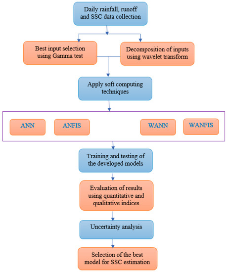
Figure 3.
Flowchart of the methodology adopted for daily suspended sediment concentration (SSC) estimation.
3. Results
3.1. Data Analysis
Different statistical parameters of original rainfall, runoff, and SSC time series used in this analysis are presented in Table 1.

Table 1.
Statistical parameters of the dataset used for daily SSC prediction.
The lower values of skewness of rainfall, runoff, and SSC were observed in both the training and testing data set. The low value of skewness is necessary for appropriate modeling. Table 2 represents the existence of a degree of correlation among rainfall (R), runoff (Q), and SSC (S) with three days lagged duration. The previous 3 days’ rainfall, runoff, and SSC were considered for applying GT based on the degree of correlation.
Table 2.
Cross-correlation matrix between different variables for daily SSC prediction.
3.2. GT for Input Selection
As the hydrologic processes are highly dynamic, the present response depends on the current response system and the past response in the hydrologic system’s memory. Hence, it is considered that present-day SSC response depends on the present day’s response of rainfall and runoff and the past three days’ response of rainfall, runoff, and SSC. The relationship between input and output variables can be expressed mathematically as:
where Rt and Qt are the present day’s rainfall and runoff, respectively. Rt − 1, Rt − 2, and Rt − 3 are the previous one, two- and three-days rainfall, respectively, Qt − 1, Qt − 2, and Qt − 3 are the previous one, two- and three-days runoff, respectively, St − 1, St − 2, and St − 3 is the previous one, two- and three-days SSC, respectively. Here, initially, a total of 11 input variables (j) were selected for GT. Based on these 11 input variables, a total of 2j − 1 (i.e., 2047) input combinations can be possible, but, in this study, reliable 58 input combinations were made and analyzed as presented in Table 3.
Table 3.
Selection of the best input combination using a Gamma test (GT).
The best input combination was selected based on minimum Gamma (Γ) and Vratio value. As per GT, the model (M14) with six input variables (Rt, Rt − 1, Rt − 2, Rt − 3, Qt, St − 1) were selected and used to develop different models.
3.3. Hydrological Model Development
3.3.1. ANN/ANFIS Models for Daily SSC Prediction
The original input variables selected by GT were directly used to construct simple ANN and ANFIS models. The schematic representation of different ANN/ANFIS models for daily SSC prediction is shown in Figure 4.
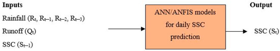
Figure 4.
Schematic representation of ANN/ANFIS models for daily SSC prediction.
In simple ANN models, the number of neurons in the single hidden layer varied from 1 to 2n + 1 (2 × 6 + 1). Hence, 13 simple ANN models were developed to assess their performance for daily SSC prediction.
3.3.2. WANN/WANFIS Models for Daily SSC Prediction
For the prediction of daily SSC using WANN/WANFIS models, the original time series data selected by GT were decomposed by applying DWT and fed as input to ANN/ANFIS models. Here, wavelet transformed data were linked to the ANN/ANFIS network to develop WANN/WANFIS models, respectively. Haar, db2, and coif2 mother wavelets were used to decompose selected six input variables into different multi-frequency sub-signals at the appropriate decomposition level. The appropriate decomposition level was selected using the suggested empirical relation as [29,42]:
where i is the appropriate decomposition level, N is the number of data points (Here, N was taken as 854 data points, and int [.] is the integer part function. Therefore, selected six input variables were decomposed at level (i) 2 using selected mother wavelets. Here, each of the selected input variables was decomposed at level 2, which produced 1 approximate (A2) and 2 detail (D1, D2) (total 3) sub-signals. Now, the best selected six input variables (i.e., Rt, Rt-1, Rt-2, Rt-3, Qt, St-1) produced 18 (6 × 3) sub-signals. Hence, these total 18 sub-signals (input variables) were fed to ANN/ANFIS to develop WANN/WANFIS models, respectively, for daily SSC prediction, as shown in Figure 5 schematically.
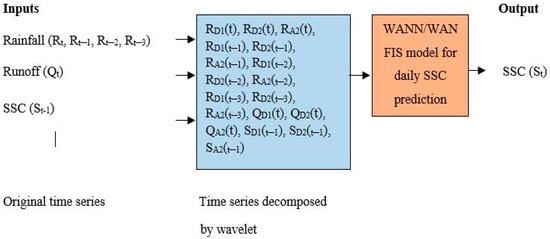
Figure 5.
Schematic representation of wavelet coupled ANN/wavelet coupled ANFIS models for daily SSC prediction.
The decomposed sub-signals of normalized rainfall, runoff, and SSC time series with selected mother wavelets at level (i) 2 are shown in Figure 6, Figure 7 and Figure 8, respectively.
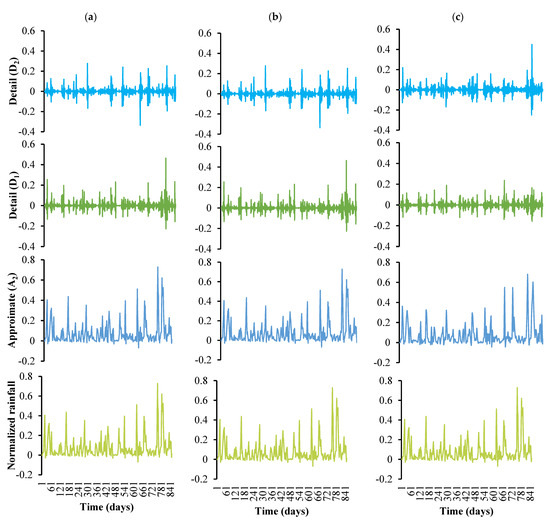
Figure 6.
Decomposition of original rainfall time series using different mother wavelets. (a) Haar, (b) db2, (c) coif2.
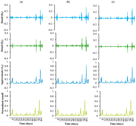
Figure 7.
Decomposition of original runoff time series using different mother wavelets. (a) Haar, (b) db2, (c) coif2.
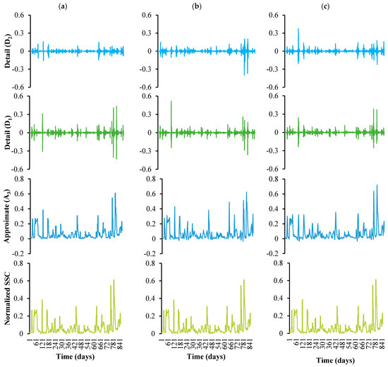
Figure 8.
Decomposition of original SSC time series using different mother wavelets. (a) Haar, (b) db2, (c) coif2.
Each sub-signal plays a different role during prediction [30]. In WANN models, the number of neurons in the hidden layer varied from 1 to 2n + 1 (2 × 18 + 1). Hence, a total of 37 WANN models per single mother wavelet were developed to assess their daily SSC prediction performance.
3.4. Quantitative Performance Evaluation of Developed Models for Daily SSC Prediction
Quantitative performance evaluation indicators like RMSE, r, WI, CE, and PARE were used to assess developed models’ predictive performance. Different AI techniques were employed for that purpose. The single best model was selected from each technique presented in Table 4 and Table 5.
Table 4.
Quantitative performance evaluation indices of the best selected Artificial Neural Network (ANN) and wavelet coupled ANN (WANN) models.
Table 5.
Quantitative performance evaluation indices of the best selected ANFIS and WANFIS models.
After comparing the quantitative performance among 13 simple ANN models, it was revealed that RMSE, r, WI, CE, and PARE varies from 0.04 g/L to 0.067 g/L and 0.078 g/L to 0.119 g/L, 0.48 to 0.83 and 0.32 to 0.75, 0.56 to 0.78 and 0.56 to 0.73, 0.063 to 0.67 and −0.016 to 0.560, −0.09% to 0.032% and −0.189% to 0.089% during training and testing, respectively. Among 13 simple ANN models, the ANN-3 model with architecture (6-3-1) was the superior model compared to others based on quantitative performance criteria. The results obtained were extremely acceptable and agree with those suggested by Rajaee [46], who applied the ANN for predicting daily SS under different time series and found that determination coefficients (R2) ranged from 0.12 to 0.87 for training and from 0.10 to 0.83 for testing datasets. Moreover, these results coincide with Sudhishri, et al. [47] observation, who investigated that ANN produced high correlations for predicting SS varied from 0.81 to 0.83. From 0.74 to 0.75 for training and validation periods, respectively. Similarly, from all 37 Haar-WANN models, it was observed that RMSE, r, WI, CE, and PARE ranges from 0.026 to 0.083 g/L and 0.069 g/L to 0.120 g/L, 0.22 to 0.93 and 0.55 to 0.85, 0.38 to 0.87 and 0.48 to 0.75, −0.454 to 0.852 and −0.039 to 0.661, −0.166% to 0.142% and −0.181% to 0.185% during training and testing, respectively. Out of 37 Haar-WANN models, the Haar-WANN-21 model with architecture (18-21-1) was selected as the best among others. The findings were parallel to Nourani and Komasi [26] results, who predicted daily multi-step ahead SS based on WANN. Their results confirmed high correlations from 0.6 to 0.89 for calibration, and from 0.55 to 0.85 for verification periods were obtained. These findings were similar to those revealed by Rajaee [46], who used several mother wavelets for daily SS simulation and stated that Haar-WANN at ANN structure (6-4-1) generated R2 0.63 RMSE of 4321 ton/day. Additionally, research outcomes are in line with those who evaluated wavelet-based ANN models for estimating daily SS and obtained a positive relationship (R2 = 0.70) between the observed–predicted data. By comparing prediction performance among 37 db2-WANN models, it was revealed that RMSE, r, WI, CE, and PARE varies from 0.015 g/L to 0.042 g/L and 0.061 g/L to 0.132 g/L, 0.81 to 0.98 and 0.43 to 0.86, 0.65 to 0.90 and 0.62 to 0.76, 0.628 to 0.952 and −0.025 to 0.734, −0.018% to 0.054% and −0.071% to 0.138% during training and testing, respectively and db2-WANN-21 model with architecture (18-21-1) was observed to be the best model for SSC prediction. These models generated more favorable outcomes compared with the results of Rajaee [46], who observed that db2-WANN at ANN structure (6-1-1) achieved R2 of 0.55 and RMSE of 4751.8 ton/day. Similarly, from all 37 coif2-WANN models, it was observed that RMSE, r, WI, CE, and PARE varies between 0.020 g/L to 0.041 g/L and 0.065 g/L to 0.120 g/L, 0.86 to 0.96 and 0.49 to 0.84, 0.69 to 0.88 and 0.62 to 0.76, 0.650 to 0.915 and −0.033 to 0.696, −0.033% to 0.056% and −0.10% to 0.123% during training and testing, respectively. By comparing all coif2-WANN models’ predictive performance, the coif2-WANN-11 model with architecture (18-11-1) was observed to be the best. These results agree with Rajaee [46], who found that the coif-WANN gave satisfactory results (R2 = 0.74, and RMSE =3601.1 ton/day) at ANN structure 4-1-1. After analyzing the quantitative prediction performance among all 48 simple ANFIS models, it was revealed that RMSE, r, WI, CE, and PARE varies between 0.033 g/L to 0.044 g/L and 0.080 g/L to 1.23 g/L, 0.77 to 0.88 and −0.43 to 0.78, 0.71 to 0.80 and 0.27 to 0.74, 0.587 to 0.772 and −107.9 to 0.545, −1 × 10⁻⁸% to 2.3 × 10⁻⁸% and −0.736% to 0.975% during training and testing, respectively. Among all 48 simple ANFIS models, the ANFIS-29 model (triangular input MF, constant output MF and 3 MFs/input) performed better during the training and testing period. Similarly, for all 48 Haar-WANFIS models, it was found that RMSE, r, WI, CE, and PARE ranges from 0.016 g/L to 0.050 g/L and 0.074 g/L to 0.288 g/L, 0.69 to 0.97 and 0.1 to 0.82, 0.63 to 0.88 and 0.5 to 0.76, 0.47 to 0.947 and −4.955 to 0.605, −4 × 10⁻⁹% to 2.5 × 10⁻⁹% and −0.105% to 0.094% during training and testing, respectively. Here, the Haar-WANFIS-27 model (triangular input MF, linear output MF, and 4 MFs/input) performed better during both the training and testing period. After comparing the prediction performance of all 48 db2-WANFIS models, it was observed that RMSE, r, WI, CE, and PARE varies between 0.012 g/L to 0.087 g/L and 0.068 g/L to 0.808 g/L, 0.11 to 0.98 and −0.51 to 0.84, 0.00 to 0.91 and 0.24 to 0.77, −0.607 to 0.969 and −45.92 to 0.666, −5 × 10⁻⁹% to 0.029% and −0.96% to 0.115% during training and testing, respectively. Here, the db2-WANFIS-25 model (triangular input MF, linear output MF and 2 MFs/input) performed better during both the training and testing period. Similarly, among all 48 coif2-WANFIS models, it was revealed that RMSE, r, WI, CE, and PARE ranges between 0.013 g/L to 0.045 g/L and 0.06 g/L to 0.392 g/L, 0.76 to 0.98 and −0.40 to 0.87, 0.69 to 0.92 and 0.41 to 0.80, 0.573 to 0.964 and −10.04 to 0.745, −5 × 10⁻⁹% to 8.9 × 10⁻⁸% and −0.398% to 0.07% during training and testing, respectively. Among all 48 coif2-WANFIS models, the coif2-WANFIS-43 model (z input MF, linear output MF and 2 MFs/input) performed better for both the training and testing period. Our results are in line with Rajaee, et al. [48], who found high linear relationships from R2 of 0.72 to 0.87 and RMSE ranged from 1805.3 ton/day to 2459.6 ton/day applying ANFIS. While the R2 was from 0.62 to 0.67, and RMSE varied from 2543 ton/day to 2838 ton/day by using WANFIS.
3.5. Qualitative Performance Evaluation of Developed Models for Daily SSC Prediction
Qualitative performance evaluation was carried out by comparing the scatter plots and time series (sediment) graphs of predicted versus observed SSC during the testing period, as shown in Figure 9 and Figure 10, respectively.
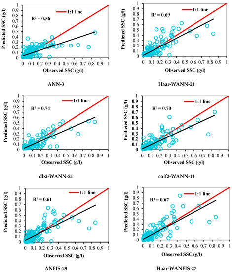
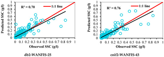
Figure 9.
Scatter plots showing the predictive performance of different models during testing.
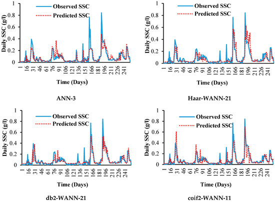
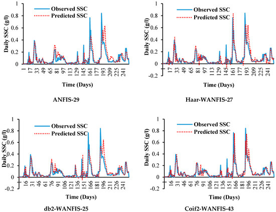
Figure 10.
Actual daily SSC versus the predicted of different models.
The best models selected from each technique as per quantitative evaluation were also assessed qualitatively to analyze their capability to capture the observed SSC time-series graph. The capability of the best-selected models for capturing low, medium, and high (peak) SSC values was examined using a time-series graph and observing the regression line’s shifting from a 1:1 line in scatter plots. Here, it was revealed that the best selected coif2-WANFIS-43 model is more accurate to capture the overall shape of the observed SSC time series. The selected coif2-WANFIS-43 model closely predicted low, medium, and high SSC values with a strong R2 of 0.76 during the testing period compared to other selected models.
All the observed and predicted data points are concentrated near the 1:1 line. The regression line is not too much shifted above or below from the 1:1 line than other models. Hence, it is revealed that the coif2-WANFIS-43 model can predict low, medium, and peak SSC values of the Koyna River basin.
3.6. Uncertainty Analysis
The strength of correlation between inputs and output determines the amount of uncertainty present in any prediction model. The amount of uncertainty incorporated in the best-selected models during the testing period is presented in Table 6.
Table 6.
Uncertainty analysis of the best-selected models during the testing period for daily SSC predictions.
Better prediction models must have small We and CIe. In this study, the coif2-WANFIS-43 model represented significantly less uncertainty in prediction, indicated by smaller We (±0.0073 g/L) and narrower CIe (0.0146 g/L) other best-selected models. All WANN models have less uncertainty than a simple ANN model for prediction purposes.
Similarly, all WANFIS models have less uncertainty than the simple ANFIS model for daily SSC prediction. Finally, it is concluded that the coif2-WANFIS-43 model is less uncertain than others. Hence, it could provide accurate daily SSC predictions. Hence, in this study, it is revealed that data pre-processing using DWT is essential to improve the model predictive accuracy.
3.7. Sensitivity Analysis
In this study, the sensitivity analysis was completed to determine the most effective hydrologic variable of the original time series data for daily SSC prediction. The best selected simple ANN-3 model was selected for detecting the critical variable. In this study, the approach given by Azamathulla, et al. [49] was used for sensitivity analysis. In this approach, a total of 10 scenarios were considered. During each scenario, the developed model performance was tested by varying the input variables one by one. During the first scenario, the developed model performance was tested by using all the input variables. During the second scenario, the developed model performance was tested by removing only one input variable and keeping all other input variables. This process of removing a single input variable and keeping all other input variables as it is was continued until the removal of all the input variables one by one and tested its performance simultaneously. The model’s predictive performance will be reduced by removing a single input variable from the selected input vector. After studying the degree of reduction in any model’s prediction performance during the absence of any single input variable, the degree of sensitivity of such an absent input variable can be determined. In this way, the essential input variable for daily SSC prediction can be determined. Hence, this approach was used here. The prediction performance observed after removing all input variables, one by one, is presented in Table 7.
Table 7.
Sensitivity analysis for detection of the most crucial variable for daily SSC prediction.
Here, it was revealed that in the absence of the previous 1-day SSC (St − 1), the selected ANN-3model’s predictive performance decreased dramatically. Therefore, it is concluded that St − 1 is the most critical hydrologic variable in the daily SSC prediction. The order of sensitivity for daily SSC prediction was observed to be St − 1 followed by Rt − 3, Rt, Rt − 2, Qt, Rt − 1.
4. Discussion
Comparison of ANN, WANN, ANFIS, and WANFIS Models for Daily SSC Prediction
The best models selected after applying different techniques were compared with each other based on quantitative and qualitative performance evaluation criteria to select the single most accurate model with high SSC prediction performance. Different performance indicators like RMSE, r, WI, CE, PARE, and R2 were used for that purpose. It was observed that WANN models performed better than simple ANN models. Among WANN models, db2-WANN models performed better than Haar- and coif2-WANN models. Similarly, WANFIS models outperformed simple ANFIS models. Among all WANFIS models, coif2-WANFIS models performed better than Haar- and db2-WANFIS models (Figure 11).
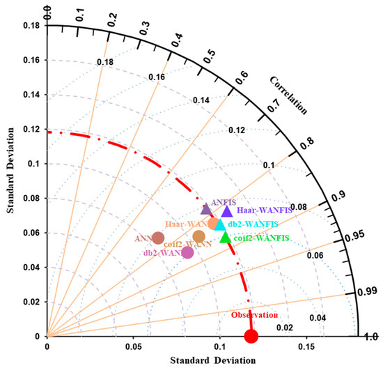
Figure 11.
Taylor diagram of the developed models for daily SSC prediction.
Here, it was revealed that the coif2-WANFIS model performed better than all other models. Here, it is observed that the wavelet-coupled hybrid models performed better than simple data-driven models. Based on sensitivity analysis, it was observed that the previous one day SSC is an essential input variable for daily SSC estimation. Koyna River basin is a very complex River basin having varying climatic and topographic conditions. Due to the complex nature of the basin, the sediment flow is highly dynamic. In this study, it is found that the coiflet mother wavelet-coupled ANFIS model is capable of predicting the highly dynamic behavior of the Koyna River basin. Hence, it can be concluded that the coiflet mother wavelet, coupled with the ANFIS model, can be able to predict the dynamic nature of the suspended sediment flow of any other complex river basin. Hence, it can be applied to other areas that have highly varying climatic and topographic conditions. Hence, the coiflet mother wavelet, coupled with the ANFIS model, is highly recommended for the river basins that come under varying climatic and topographic conditions.
5. Conclusions
In this study, the predictive performances of simple and wavelet-coupled AI models were analyzed for daily SSC prediction. In this study, 124 ANN/WANN and 192 ANFIS/WANFIS models were developed to predict daily SSC and tested their predictive performance. The developed models’ capability to capture the observed sediment graph at low, medium, and peak SSC was evaluated. Finally, it is revealed that the hybrid wavelet-coupled AI models can model non-linear behavior between inputs and output variables.
Hybrid AI models outperformed simple AI models. Hydrologic processes such as runoff flow and sediment flow are highly complex and non-stationary; hence data pre-processing with DWT receives too much importance. Here, it was observed that simple AI models like ANN or ANFIS could not precisely model the hydrologic process without pre-processing original time series data. Out of 316 models, the coif2-WAFIS-43 model performed better based on quantitative and qualitative performance evaluation criteria. Hence, it could be applied for daily SSC prediction of the Koyna River basin. The final selected model is better, consistent, and accurate for daily SSC predictions among all other models. The reliability of the developed models was evaluated using uncertainty analysis. Here, it was revealed that simple AI models’ reliability increased after coupling it with wavelet transform. The uncertainty analysis also indicated that the coif2-WAFIS-43 model is more reliable than others for daily SSC prediction. St-1 input variable was observed to be the most critical input variable, followed by Rt-3, Rt, Rt-2, Qt, Rt-1 for daily SSC modeling based on sensitivity analysis.
Here, in this study, it was found that the coiflet wavelet-coupled ANFIS model can predict sediment flow of highly complex river basin with varying climatic and topographic conditions. Hence, it is concluded that a coiflet mother wavelet, coupled with the ANFIS model, is more capable of modeling the dynamic behavior of complex river basins like the Koyna River basin. The future study should be focused on investigating the validity of this approach for multiple time steps (1, 2, 3 days/months ahead) SSC prediction. The impact of some additional inputs such as rainfall intensity, soil moisture content, maximum and minimum temperature, wind speed, relative humidity, bright sunshine hours, etc., should be assessed to improve the model’s predictive efficiency. The applicability of other AI models like a genetic algorithm (GA), support vector machine (SVM), and wavelet-coupled SVM should be investigated to improve the prediction performance. Further, the result of the hybrid mentioned above approach should also be verified by selecting only those sub-signals with a higher correlation to output.
Author Contributions
Conceptualization, T.S.B. and P.K.; methodology, T.S.B. and P.K.; software, T.S.B., M.K., and P.K.; validation, T.S.B. and P.K.; formal analysis, T.S.B., P.K., A.E., and A.K.; investigation, T.S.B., P.K., A.E., and A.K.; writing—original draft preparation, T.S.B. and M.K.; writing—review and editing, T.S.B., P.K., M.K., and A.K.; visualization, T.S.B., P.K., A.E., and A.K.; supervision, P.K., A.E., and A.K.; project administration, A.K. funding acquisition, A.K. All authors have read and agreed to the published version of the manuscript.
Funding
This research received no external funding.
Institutional Review Board Statement
Not applicable.
Informed Consent Statement
Not applicable.
Acknowledgments
The authors would like to thank the anonymous reviewers for their valuable comments and suggestions to improve this manuscript further. Alban Kuriqi was supported by a Ph.D. scholarship granted by Fundação para a Ciência e a Tecnologia, I.P.P (FCT), Portugal the Ph.D. Program FLUVIO—River Restoration and Management, grant number: PD/BD/114558/2016.
Conflicts of Interest
The authors declare no conflict of interest.
Appendix A
The activation function f reduces the amplitude of output and show its non-linearity in the form given as:
The neurons’ performance can be altered by varying the transfer functions and changing the parameter like thresholds or gains. The processing at particular neurons occurs independently of all the other neurons of a given network. The processing completed at particular neurons can affect the whole neural network at the same time because the output of that particular neuron becomes an input to many other neurons of a neural network. Similarly, the neural network learns by changing the connection weights between the neurons. By using a suitable learning algorithm, the connection weights are altered using the training data set. The weights are frozen after the completion of learning. A feed-forward Multilayer Perceptron (MLP) neural network is the most widely used neural network in hydrology [11]. In the feed-forward network, the input vector is first forwarded to the output layer through a hidden layer using a non-linear transfer function that may be differentiable, continuous, or bounded. The output layer’s error between simulated output and target output is propagated to adjust weights through some training mechanism. This process of “feed-forward” and “error back-propagation” is repeated until there is an acceptable reduction in error.
Appendix B
Layer 1: Every node in this layer creates a membership grade for an input variable. Every node i in this layer is a square node (or adaptive node), whose node function is defined as:
where (x or y) is the input to the ith node, Ai (or Bi−2) is the fuzzy set associated with this node, and it is characterized by MFs shape. The MF may be any appropriate functions (continuous and piecewise differentiable) like Gaussian, Trapezoidal, Generalized bell, and Triangular shaped functions. Different researchers apply different MFs for the search for the solution to any problem. Considering, generalized bell function, the output of the first layer (ith node) is determined as:
where (ai, bi, ci) is the premise parameter set, and by varying this premise parameter, the shape of MF can change. For a Gaussian function, the output of the first layer (ith node) is determined as:
where (ci or σi) is the premise parameter set, and by varying this premise parameter, the shape of MF can change. Here, MFs center is represented by c while MFs width is represented by σ.
Layer 2: Every node in this layer is a fixed node labeled as II, whose output multiplicate all incoming signals. The output Oi2 indicates the firing strength of a rule, and it can be determined as:
Layer 3: Every node in this layer is a fixed node labeled as N. The ith node in this layer determines the normalized firing strengths as:
Layer 4: Every node i in this layer is a square node with a node function given as:
where is a normalized firing strength obtained in layer 3 and {pi, qi, ri} is the parameter set of this node (consequent parameters).
Layer 5: The single node in this layer is a fixed node labeled as sigma that computes the overall output as the summation of all incoming signals,
The single fixed node of this layer computes the final output by adding the entire incoming signal. In this manner, the input vector can be fed layer by layer into the ANFIS structure. The ANFIS uses a hybrid algorithm as a learning model for training, representing a combination of the least square and gradient descent method. The consequent parameters {pi, qi, ri} and premise parameters {ai, bi, ci} are required to be optimized. Consequent parameters are identified using the least square method during the forward pass of the hybrid learning approach when the node outputs move forward. The error signals are propagated backward during the backward pass. The premise parameters are adjusted by using the gradient descent method [22].
Appendix C
Gamma statistic Γ defines the determination of such a part of output variance, which cannot be accounted for in the smooth data model. Let, bT[i,k] represents kth (1 ≤ k ≤ p) nearest neighbor, in terms of Euclidean distance to bi(1 ≤ I ≤ N). GT derived from Delta function of the input vector is given as:
where |….| is the Euclidean distance and corresponding output values Gamma function is denoted as:
After applying the least square regression analysis, Γ value can be determined through p points (i.e., δN (k), γN(k)) which is given as:
The intercept on the vertical axis (δ = 0) gives the Γ value. It can be indicated as:
ΓN (k) Var (s) in probability as δN (k) 0
To standardize the results, another term, Vratio, can be used. It ranges from 0 to 1, and it is defined as:
where σ2(c) represents the variance of output (c). The value of Vratio closer to 1 represents a higher degree of predictability.
Appendix D
Appendix D.1. Root Mean Squared Error (RMSE)
It is an indicator of determining the prediction accuracy of any model. It compares the values of observation versus prediction and finds the difference between them. RMSE represents how the data points are spread around the line of the best fit. It also measures the average magnitude of the error. It gives positive value ranges between 0 to ∞. For a perfect fit between observed and predicted values, the RMSE is zero. In contrast, the value of RMSE increases as the deviation increases between observed and predicted values [50]. RMSE can be calculated using the relationship as:
Qo is the observed value, Qp is the predicted value, and n is the total number of values.
Appendix D.2. The Correlation Coefficient (r)
It shows the degree of closeness between observed and predicted values. It will be zero only if predicted, and observed values are entirely independent of each other. It can be determined using the following formula:
where is the average of the observed values, is the average of the predicted values.
Appendix D.3. Willmott Index (WI)
Willmott (1981) first invented the Willmott index (index of agreement) to overcome the insensitivity of the coefficient of determination (R2) and Nash-Sutcliffe efficiency. WI lies between 0 to 1; the higher WI values indicate that predicted values show better agreement than observed values. Legates and McCabe Jr. [51] introduced a modified WI followed by a generic form of WI proposed by Willmott [52] to overcome the limitations of original WI against extreme values, which is expressed as:
where is the average of the observed values. The advantage of modified WI is that the errors and differences are not inflated. Their squared values and differences and weights are provided with their appropriate weights. The modified WI also varies from 0 to 1, and the higher values indicate a better fitting model.
References
- Kuriqi, A.; Koçileri, G.; Ardiçlioğlu, M. Potential of Meyer-Peter and Müller approach for estimation of bed-load sediment transport under different hydraulic regimes. Model. Earth Syst. Environ. 2020, 6, 129–137. [Google Scholar] [CrossRef]
- Ardıçlıoğlu, M.; Kuriqi, A. Calibration of channel roughness in intermittent rivers using HEC-RAS model: Case of Sarimsakli creek, Turkey. SN Appl. Sci. 2019, 1, 1080. [Google Scholar] [CrossRef]
- Adnan, R.M.; Liang, Z.; El-Shafie, S.; Zounemat, K.; Kisi, O. Prediction of Suspended Sediment Load Using Data-Driven Models. Water 2019, 11, 2060. [Google Scholar] [CrossRef]
- Melesse, A.M.; Ahmad, S.; McClain, M.E.; Wang, X.; Lim, Y.H. Suspended sediment load prediction of river systems: An artificial neural network approach. Agric. Water Manag. 2011, 98, 855–866. [Google Scholar] [CrossRef]
- Towfiqul Islam, A.R.M.; Talukdar, S.; Mahato, S.; Kundu, S.; Eibek, K.U.; Pham, Q.B.; Kuriqi, A.; Linh, N.T.T. Flood susceptibility modelling using advanced ensemble machine learning models. Geosci. Front. 2020. [Google Scholar] [CrossRef]
- Kuriqi, A.; Pinheiro, A.N.; Sordo-Ward, A.; Garrote, L. Water-energy-ecosystem nexus: Balancing competing interests at a run-of-river hydropower plant coupling a hydrologic-ecohydraulic approach. Energy Convers. Manag. 2020, 223, 113267. [Google Scholar] [CrossRef]
- Buyukyildiz, M.; Kumcu, S.Y. An Estimation of the Suspended Sediment Load Using Adaptive Network Based Fuzzy Inference System, Support Vector Machine and Artificial Neural Network Models. Water Resour. Manag. 2017, 31, 1343–1359. [Google Scholar] [CrossRef]
- Kisi, O. Suspended sediment estimation using neuro-fuzzy and neural network approaches/Estimation des matières en suspension par des approches neurofloues et à base de réseau de neurones. Hydrol. Sci. J. 2005, 50, 696. [Google Scholar] [CrossRef]
- Kumari, A.; Kumar, M.; Kumar, A.; Amitabh, A. Daily Gauge-Discharge Simulation using ANN and Wavelet-ANN Models for Muri Station, Jharkhand. Indian J. Ecol. 2020, 47, 645–649. [Google Scholar]
- Zhu, Y.-M.; Lu, X.X.; Zhou, Y. Suspended sediment flux modeling with artificial neural network: An example of the Longchuanjiang River in the Upper Yangtze Catchment, China. Geomorphology 2007, 84, 111–125. [Google Scholar] [CrossRef]
- Olyaie, E.; Banejad, H.; Chau, K.-W.; Melesse, A.M. A comparison of various artificial intelligence approaches performance for estimating suspended sediment load of river systems: A case study in United States. Environ. Monit. Assess. 2015, 187, 189. [Google Scholar] [CrossRef] [PubMed]
- Güldal, V.; Tongal, H. Comparison of Recurrent Neural Network, Adaptive Neuro-Fuzzy Inference System and Stochastic Models in Eğirdir Lake Level Forecasting. Water Resour. Manag. 2010, 24, 105–128. [Google Scholar] [CrossRef]
- Valizadeh, N.; El-Shafie, A. Forecasting the Level of Reservoirs Using Multiple Input Fuzzification in ANFIS. Water Resour. Manag. 2013, 27, 3319–3331. [Google Scholar] [CrossRef]
- Samantaray, S.; Ghose, D.K. Assessment of Suspended Sediment Load with Neural Networks in Arid Watershed. J. Inst. Eng. Ser. A 2020, 101, 371–380. [Google Scholar] [CrossRef]
- Rajaee, T.; Jafari, H. Two decades on the artificial intelligence models advancement for modeling river sediment concentration: State-of-the-art. J. Hydrol. 2020, 588, 125011. [Google Scholar] [CrossRef]
- Meshram, S.G.; Singh, V.P.; Kisi, O.; Karimi, V.; Meshram, C. Application of Artificial Neural Networks, Support Vector Machine and Multiple Model-ANN to Sediment Yield Prediction. Water Resour. Manag. 2020, 34, 4561–4575. [Google Scholar] [CrossRef]
- Kumar, M.; Kumar, P. Daily Suspended-sediment Concentration simulation using ANN and Wavelet ANN models. Int. Arch. Appl. Sci. Technol. 2019, 11, 60–69. [Google Scholar]
- Hussan, W.; Khurram Shahzad, M.; Seidel, F.; Nestmann, F. Application of Soft Computing Models with Input Vectors of Snow Cover Area in Addition to Hydro-Climatic Data to Predict the Sediment Loads. Water 2020, 12, 1481. [Google Scholar] [CrossRef]
- Talebizadeh, M.; Morid, S.; Ayyoubzadeh, S.A.; Ghasemzadeh, M. Uncertainty Analysis in Sediment Load Modeling Using ANN and SWAT Model. Water Resour. Manag. 2010, 24, 1747–1761. [Google Scholar] [CrossRef]
- Malik, A.; Kumar, A.; Kisi, O.; Shiri, J. Evaluating the performance of four different heuristic approaches with Gamma test for daily suspended sediment concentration modeling. Environ. Sci. Pollut. Res. 2019, 26, 22670–22687. [Google Scholar] [CrossRef]
- Yin, D.; Shu, L.; Chen, X.; Wang, Z.; Mohammed, M.E. Assessment of Sustainable Yield of Karst Water in Huaibei, China. Water Resour. Manag. 2011, 25, 287–300. [Google Scholar] [CrossRef]
- Seo, Y.; Kim, S.; Kisi, O.; Singh, V.P. Daily water level forecasting using wavelet decomposition and artificial intelligence techniques. J. Hydrol. 2015, 520, 224–243. [Google Scholar] [CrossRef]
- Singh, V.K.; Kumar, D.; Kashyap, P.S.; Kisi, O. Simulation of suspended sediment based on gamma test, heuristic, and regression-based techniques. Environ. Earth Sci. 2018, 77, 708. [Google Scholar] [CrossRef]
- Agarwal, A.; Mishra, S.K.; Ram, S.; Singh, J.K. Simulation of Runoff and Sediment Yield using Artificial Neural Networks. Biosyst. Eng. 2006, 94, 597–613. [Google Scholar] [CrossRef]
- Dadaser-Celik, F.; Cengiz, E. A neural network model for simulation of water levels at the Sultan Marshes wetland in Turkey. Wetl. Ecol. Manag. 2013, 21, 297–306. [Google Scholar] [CrossRef]
- Nourani, V.; Komasi, M. A geomorphology-based ANFIS model for multi-station modeling of rainfall–runoff process. J. Hydrol. 2013, 490, 41–55. [Google Scholar] [CrossRef]
- Samantaray, S.; Ghose, D.K. Evaluation of suspended sediment concentration using descent neural networks. Procedia Comput. Sci. 2018, 132, 1824–1831. [Google Scholar] [CrossRef]
- Lohani, A.K.; Goel, N.K.; Bhatia, K.K.S. Improving real time flood forecasting using fuzzy inference system. J. Hydrol. 2014, 509, 25–41. [Google Scholar] [CrossRef]
- Alizadeh, M.J.; Kavianpour, M.R.; Kisi, O.; Nourani, V. A new approach for simulating and forecasting the rainfall-runoff process within the next two months. J. Hydrol. 2017, 548, 588–597. [Google Scholar] [CrossRef]
- Ravansalar, M.; Rajaee, T. Evaluation of wavelet performance via an ANN-based electrical conductivity prediction model. Environ. Monit. Assess. 2015, 187, 366. [Google Scholar] [CrossRef]
- Shoaib, M.; Shamseldin, A.Y.; Melville, B.W. Comparative study of different wavelet based neural network models for rainfall–runoff modeling. J. Hydrol. 2014, 515, 47–58. [Google Scholar] [CrossRef]
- Shoaib, M.; Shamseldin, A.Y.; Khan, S.; Khan, M.M.; Khan, Z.M.; Sultan, T.; Melville, B.W. A Comparative Study of Various Hybrid Wavelet Feedforward Neural Network Models for Runoff Forecasting. Water Resour. Manag. 2018, 32, 83–103. [Google Scholar] [CrossRef]
- Grossmann, A.; Morlet, J. Decomposition of Hardy Functions into Square Integrable Wavelets of Constant Shape. Fundam. Pap. Wavelet Theory 1984, 15, 723–736. [Google Scholar] [CrossRef]
- Kisi, O. Wavelet Regression Model as an Alternative to Neural Networks for River Stage Forecasting. Water Resour. Manag. 2011, 25, 579–600. [Google Scholar] [CrossRef]
- Partal, T.; Kişi, Ö. Wavelet and neuro-fuzzy conjunction model for precipitation forecasting. J. Hydrol. 2007, 342, 199–212. [Google Scholar] [CrossRef]
- Nayak, P.C.; Venkatesh, B.; Krishna, B.; Jain, S.K. Rainfall-runoff modeling using conceptual, data driven, and wavelet based computing approach. J. Hydrol. 2013, 493, 57–67. [Google Scholar] [CrossRef]
- Prahlada, R.; Deka, P.C. Forecasting of Time Series Significant Wave Height Using Wavelet Decomposed Neural Network. Aquat. Procedia 2015, 4, 540–547. [Google Scholar] [CrossRef]
- Hassan, M.; Ali Shamim, M.; Sikandar, A.; Mehmood, I.; Ahmed, I.; Ashiq, S.Z.; Khitab, A. Development of sediment load estimation models by using artificial neural networking techniques. Environ. Monit. Assess. 2015, 187, 686. [Google Scholar] [CrossRef]
- Kişi, Ö. Daily suspended sediment estimation using neuro-wavelet models. Int. J. Earth Sci. 2010, 99, 1471–1482. [Google Scholar] [CrossRef]
- Genç, O.; Kişi, Ö.; Ardıçlıoğlu, M. Determination of Mean Velocity and Discharge in Natural Streams Using Neuro-Fuzzy and Neural Network Approaches. Water Resour. Manag. 2014, 28, 2387–2400. [Google Scholar] [CrossRef]
- Sharghi, E.; Nourani, V.; Najafi, H.; Molajou, A. Emotional ANN (EANN) and Wavelet-ANN (WANN) Approaches for Markovian and Seasonal Based Modeling of Rainfall-Runoff Process. Water Resour. Manag. 2018, 32, 3441–3456. [Google Scholar] [CrossRef]
- Nourani, V.; Kisi, Ö.; Komasi, M. Two hybrid Artificial Intelligence approaches for modeling rainfall–runoff process. J. Hydrol. 2011, 402, 41–59. [Google Scholar] [CrossRef]
- Ebtehaj, I.; Bonakdari, H. Performance Evaluation of Adaptive Neural Fuzzy Inference System for Sediment Transport in Sewers. Water Resour. Manag. 2014, 28, 4765–4779. [Google Scholar] [CrossRef]
- Jang, J.R. ANFIS: Adaptive-network-based fuzzy inference system. IEEE Trans. Syst. Man Cybern. 1993, 23, 665–685. [Google Scholar] [CrossRef]
- Nash, J.E.; Sutcliffe, J.V. River flow forecasting through conceptual models part I—A discussion of principles. J. Hydrol. 1970, 10, 282–290. [Google Scholar] [CrossRef]
- Rajaee, T. Wavelet and ANN combination model for prediction of daily suspended sediment load in rivers. Sci. Total Environ. 2011, 409, 2917–2928. [Google Scholar] [CrossRef]
- Sudhishri, S.; Kumar, A.; Singh, J.K. Comparative Evaluation of Neural Network and Regression Based Models to Simulate Runoff and Sediment Yield in an Outer Himalayan Watershed. J. Agric. Sci. Technol. 2016, 18, 681–694. [Google Scholar]
- Rajaee, T.; Mirbagheri, S.A.; Nourani, V.; Alikhani, A. Prediction of daily suspended sediment load using wavelet and neurofuzzy combined model. Int. J. Environ. Sci. Technol. 2010, 7, 93–110. [Google Scholar] [CrossRef]
- Azamathulla, H.M.; Haghiabi, A.H.; Parsaie, A. Prediction of side weir discharge coefficient by support vector machine technique. Water Supply 2016, 16, 1002–1016. [Google Scholar] [CrossRef]
- Kumar, M.; Kumari, A.; Kushwaha, D.P.; Kumar, P.; Malik, A.; Ali, R.; Kuriqi, A. Estimation of Daily Stage–Discharge Relationship by Using Data-Driven Techniques of a Perennial River, India. Sustainability 2020, 12, 7877. [Google Scholar] [CrossRef]
- Legates, D.R.; McCabe, G.J., Jr. Evaluating the use of “goodness-of-fit” Measures in hydrologic and hydroclimatic model validation. Water Resour. Res. 1999, 35, 233–241. [Google Scholar] [CrossRef]
- Willmott, C.J. On the Evaluation of Model Performance in Physical Geography. In Spatial Statistics and Models; Gaile, G.L., Willmott, C.J., Eds.; Springer: Dordrecht, The Netherlands, 1984; pp. 443–460. [Google Scholar] [CrossRef]


Publisher’s Note: MDPI stays neutral with regard to jurisdictional claims in published maps and institutional affiliations. |
© 2021 by the authors. Licensee MDPI, Basel, Switzerland. This article is an open access article distributed under the terms and conditions of the Creative Commons Attribution (CC BY) license (http://creativecommons.org/licenses/by/4.0/).