Abstract
The search for simple models of drainage–irrigation systems functioning and management has still been an important research objective. Therefore, we presented a conceptual model based on groundwater dynamics equation along with proper assumptions on water equivalent of transient porosity-i.e., storage in the soil profile based on the long-term experience of the research on drainage-sub-irrigation systems. Several parameters have been incorporated in the model to effectively and comprehensively describe drainage/irrigation time, leakage from the soil profile, the soil moisture content in the root zone, and the shape of the groundwater table on the drainage–sub-irrigation plot. The model was successfully validated on groundwater level data in ditch midspacing on an experimental site located within a valley sub-irrigation system with the advantage of a relatively simple representation of flows through the soil profile. The robust character of the conceptual equation of groundwater dynamics, as well as the approach to its’ parameters, were proved through a close match between the model and observations. This promotes the capacities of the proposed modeling procedure to conceptualize drainage-irrigation development with the impact of external and internal sources of water. The potential was offered for the evaluation of water management practices in a valley system influenced by horizontal inflows from surrounding areas as indicated by calibration results. Future challenges were revealed in terms of water exchange between the plots and validation of soil moisture content modeling.
1. Introduction
The quantitative description of physical, chemical, and biological interactions in soils at multiple scales and degree of achievement has been an established goal and key challenge in soil and water sciences. The earliest numerical and analytical models date back to the last century referring mainly to the simulation of water flow [1], heat flow [2], solute transport processes [3], soil organic carbon [4], and nutrient dynamics [5]. These models consisted mostly of analytical solutions of partial differential equations for well-defined soils and porous media, numerical solutions of single partial differential equations, or respective conceptual models dedicated to soil water management [6]. Along with the considerable progress from early modeling efforts, fundamental soil processes and their interactions have become well recognized and documented with some considerations remaining, such as drainage-irrigation impact and maintenance [7,8,9,10,11].
The contemporary research field which still deserves attention and searches for innovative solutions is the drainage-irrigation scheduling including the parameters that can effectively delineate the process [11,12]. For this purpose, we demonstrated a conceptual model developed in the original work of E.Kaca [11]. It is based on drainage/irrigation time constant and specific yield as conditioning groundwater table dynamics along with proper assumptions on fluxes through water table in the soil profile and so-called water equivalent (temporary water reserves in the soil). Its suitability was presented on the lowland Central Poland sub-irrigation system for the sake of possible alterations to water table management and a search for more simple models of drainage-irrigation practices development.
2. Materials and Methods
2.1. Study Site
The research was focused on drainage-irrigation plot no. F2, located in Central Poland lowland valley area (Mazovia voivodship, Góra Kalwaria commune, Solec village, N 52°02′ 22,5276″ E 21°05′ 46,8672′′). That plot became part of a typical sub-irrigation system, constructed between 1941 and 1943 and finally put into operation in 1967, utilized as grassland throughout the research period 2015–2017. The main watercourse of that system-the Mała river (catchment area of 72.8 km2) was designated as a source of water for irrigation and supplier A served for water distribution (Figure 1).
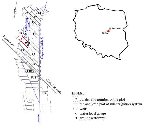
Figure 1.
Drainage-irrigation system and the research plot near Solec town.
Drainage- irrigation ditch spacing varied from 90 to 130 m, and average design depth equaled 100 cm. They were located in the valley and typically linked the river and the supplier to secure proper hydrologic conditions and water requirements for prevailing grassland farming [13]. At the analyzed plot, surface water levels in the Mała river were controlled by the weir and gauged on-site as well as groundwater tables in the distance of 60 m from the river measured on the daily interval (Figure 1).
The soil of the study site involved fen peat with a thickness equal to 0.9 m, mainly sedge (Cariceti) and sedge-reed (Cariceto-Phragmiteti) of the medium and high degree of decomposition and underlain with heavy clay. According to the WRB system, the soil was classified as Rheic Hemic Histosol (Drainic) [14].
Horizontal, saturated hydraulic conductivity of the analyzed fen soil ranged from 1.07 to 1.2 m/day as indicated by direct field measurements [15] while vertical ones estimated in laboratory conditions [16] varied from 0.5 to 0.7 m/day. Soil bulk density reached 0.28 g/cm3 on average with standard deviation of 0.02 g/cm3 while mean particle density equaled 1.67 g/cm3 with standard deviation of 0.09 g/cm3 and Θs—saturated soil moisture content of 0.84 [m3/m3] (std. dev. = 0.01 m3/m3).
2.2. Meteorological Indicators
The weather conditions were recorded at the meteorological station located in the field site. The main purpose of the weather parameter measurements was to determine reference evapotranspiration (Equation (1)). The precipitation was measured with an automatic A-Ster TPG 124 tipping-bucket gauge. All meteorological parameters required for estimates of reference evapotranspiration by Penman-Monteith method [17] including wind speed, air temperature, relative humidity, and sunshine duration were measured by A-Ster, HT-125 type automatic weather station.
Long–term monthly precipitation (1960–2017) was obtained from the nearby meteorological station of Warsaw University of Life Sciences, located in Ursynów district in Warsaw (Table 1).
where:

Table 1.
Distribution of the precipitation data in the years from 2015 to 2017 in the light of the long-term precipitation record.
- ETo—reference evapotranspiration [mm day−1],
- Rn—net radiation at the crop surface [MJ m−2 day−1],
- G—soil heat flux density [MJ m−2 day−1],
- T—mean daily air temperature at 2 m height [°C],
- u2—wind speed at 2 m height [m s−1],
- es—saturation vapor pressure [kPa],
- es − ea—saturation vapor pressure deficit [kPa],
- ∆—slope vapor pressure curve [kPa °C−1],
- γ—psychrometric constant [kPa °C−1].
On the other hand, precipitation totals were estimated for consecutive months (April–October) of years 2015–2017 and the RPI- (Relative Precipitation Index) [18] was used as an accepted indicator of precipitation shortage either excess in meteorological studies (Equation (2)):
where P—monthly precipitation (mm), Pavg—mean, long-term monthly precipitation (mm).
Mean monthly long-term precipitation totals (1960–2017) revealed a gradual increase from April to July, but then they decreased reaching finally the lowest value in October, nearly identical to April. It should be stressed, however, that the highest precipitation totals occurred in the summer from June to August (Table 1).
Monthly precipitation distribution in the analyzed years 2015–2017 was different from the long-term one. The observed totals for the period April–October were equal to 309.7 mm in 2015, 334.7 mm in 2016, and 564.9 in 2017, respectively, while the long-term mean (1960–2017) equaled 396.7 mm. The highest precipitation totals in the research period were observed for autumn months: October 2016 and September 2017 and they were considerably higher from long-term ones. At the same time, the observation period in 2017 (except for September) exhibited the monthly totals closest to long-term values.
Exceptionally lowest precipitation was observed for August 2015 (7.4 mm) in comparison to long-term one (64.6 mm), however, the highest monthly values occurred in September of 2016 and October of 2016 and 2017, considerably exceeding the long-term averages.
One of the frequently used indicators of atmospheric drought is the relative precipitation index (RPI) [19]. Basing on the data given in Table 1, the years 2015–2016 can be estimated as dry, while 2017 as the average year.
The analyzed reference evapotranspiration reached the highest daily values in July and August of 2015 (3–5 mm/day) and in October were subject to decrease to 1–2 mm/day. In 2016 generally lower evapotranspiration values were observed, reaching the maximum ones in August (3–4 mm/day). In 2017, however, daily evapotranspiration values were the lowest in comparison to other observation periods (2015–2016). Total reference evapotranspiration for the whole period April–October reached 717 mm in 2015, 669 mm in 2016, and 608 mm in 2017, respectively.
2.3. Model Description
The main part of the proposed model of drainage-irrigation (sub-irrigation) functioning can be expressed as a conceptual equation of groundwater table dynamics [11] in the following form:
where:
- j = number of the current moment of calculation,
- = the computation interval of time, e.g., day
- n = natural number and zero; τ = n · Δt = time-lag of irrigation or drainage [T],
- T = the time constant of drainage/irrigation [T],
- = the specific yield in soil profile [-],
- = groundwater table level midspacing between the ditches/drain pipes without taking into account deep percolation of soil water, at the moment j + 1 [L],
- = initial condition-groundwater table level midspacing between the ditches/drain pipes after taking into account deep percolation of soil water, at the moment j [L],
- = inducing factors–the water table level in the ditches/in the soil at the lines of the drain pipes in moment j + 1 − n and j − n, respectively.
- = the average level of groundwater at any given time without taking into account deep percolation of soil water [L],
- = the water level in the ditches/in the line of the drain pipes and the groundwater level midspacing between the ditches/drain pipes, respectively, at the cross-section without taking into account deep percolation of soil water [L],
- = coefficient of the shape of the groundwater table curve between the ditches/drain pipes [-],
- ET = flux density of evapotranspiration at the cross-section [LT−1],
- = flux density of effective precipitation and effective sprinkler irrigation rate (infiltration into the unsaturated zone) [LT−1],
- = depth beneath the land surface to the reference level [L],
- = the depth of the root zone of plants in the soil profile [L],
- = water exchange coefficient between the aquifers [T−1],
- = the net lateral flux density of water in horizontal subsurface flow exchanged with adjacent areas (released from or taken into soil storage) [LT−1].
The level of groundwater after the deep percolation of soil water midspacing between the ditches/drain pipes is calculated from the formulas (Figure 2):
where:
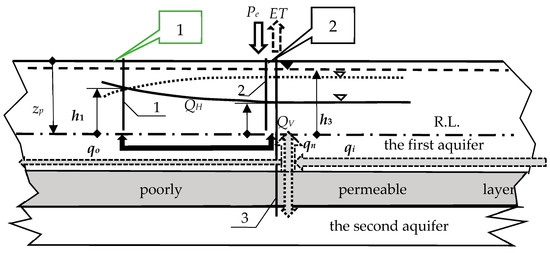
Figure 2.
Cross-section through the field perpendicular to two ditches/drains: 1 and 2—observation wells; 3—piezometer, qn—net lateral exchange of groundwater from adjacent areas (qn = qi − qo).
- = coefficient of the additional water storage capacity of the root zone and soil surface [-],
- = corrected (after soil water deep percolation) water equivalent of transient porosity in the soil profile at j + 1 moment,
- = drainable porosity; ; = maximum value of specific yield [-].
The corrected water equivalent of transient porosity, , is expressed by the relationship:
- = water equivalent of transient porosity in the soil profile at j + 1 moment-corrected (after soil water deep percolation),
- = total specific yield of the soil [L].
The water equivalent of transient porosity can be presented in the following algebraic form:
where: rainfall shortage in the period from tj to tj+1 [L]
In Equations (14) and (15) the relations between δ and the groundwater table level h can be presented as follows:
where: .
As the model requires the input of the water equivalent of transient porosity (Equations (10)–(13)) which starting values are relatively difficult to identify, the resultant average soil moisture of the soil root zone was incorporated into the modeling procedure. This also generates the possibility of the model to compute soil moisture content either use it in the calibration process. The average soil moisture of the root layer of the thickness of za, along with the groundwater table level, hj+1, is given by the following equation:
where:
- = average soil moisture of the root layer of thickness za [L3 L−3],
- = average saturated soil moisture of the root layer of thickness za [L3 L−3],
- = transient porosity below the layer of the main mass of plant roots about thickness za.
The value is described by the following formulas:
2.4. Model Calibration and Validation
The calibration of model parameters was carried out with the method of numeric optimization (non-gradient Hooke–Jeeves algorithm) with introduced limitations on the values of parameters using a series of groundwater level observations- measured in the field site. Hooke and Jeeves algorithm [20] is used to search the optimum values of the process variables. That algorithm incorporates the past history of a sequence of iterations into the generation of a new search direction. It establishes combinations of exploratory moves with pattern moves. The exploratory moves examine the local behavior of the function and seek to locate the direction of so-called stepping valleys that might be present. Finally, the process is finished when the minimalized criterion value of the average approximation error (standard deviation of residual values) is achieved:
where:
- N = the number of results of measurements and the number of results of calculations taken for comparisons,
- = calculated and measured values, respectively.
The values stand herein for the mean level of water or alternatively for moisture content in the root zone of the soil in midspacing between the ditches, calculated and measured in the sub-irrigation plot, respectively. Specific yield—µ, T—drainage/irrigation time constant, coefficient of the additional water storage capacity, -water exchange coefficient between the aquifers, average saturated soil moisture were subject to calibration in the first instance. Their value range was assumed based on literature data [13,21] but in the case of T previous estimates available for the research area were used [13]. Additionally, the S parameter was set to a reasonably low value for the sake of calibration as suggested by relevant literature in the case of poorly permeable, basal, heavy clay [22]. The second calibration target was set for qn—net lateral exchange of groundwater from adjacent areas, so the research plot was situated in the middle of a river valley for which this could be the case.
The essential verification of Equation (3) was done by comparing the results of calculations with the results of measurements for an independent dataset that was not used for the calibration of parameters. Again, the average error was utilized to assess the quality of the validation process (Equation (20)). The visual comparisons of the modeled and observed groundwater tables were used to assess the goodness of fit of parameter values.
3. Results and Discussion
3.1. Estimation of Model Performance
The conceptual model was used herein in an attempt to compute groundwater levels in midspacing of the ditches within the drainage–irrigation (sub-irrigation) plot. The modeling results were supported by necessary, specific assumptions on recharging fluxes (equations for upward or downward aquifer seepage), specific yield estimation basing on groundwater heads, and finally assumptions on water equivalent of transient porosity (volume of leakage from the soil profile for a given time step). This is found to be a sample case for this kind of model, that relates ditch or river water level to groundwater table position measured in a particular spot (ditch or drain midspacing) except for the potential for other water management problems. A point should be made, that the resultant groundwater tables (h2) are obtained through Equation (3), developed further into Equation (10) for which the starting values of the water equivalent were approached through soil moisture content (volumetric content by Equation (16). The values of the soil moisture content were known from gravimetric sampling at the beginning of each analyzed period (2015–2017) and are required every time to launch the calculations even if the moisture content is not explicitly modeled, which was the case herein.
It should be also stated, that we utilized groundwater table dynamics equation (Equation (3)) for the case of drainage/irrigation (sub-irrigation) plot taking into account also the net, horizontal subsurface flow exchanged with adjacent areas (released from or taken into soil storage). This particular situation is assumed to be valid for river valleys, such that the horizontal flow values are not simple in identification or unknown, and must be adjusted during model calibration. Summing up, the testing phase of the proposed model involved the sub-irrigation plot on a fen peat soil, also accounting for the lateral inflow e.g., hydrological feeding from surrounding uplands in particular.
Calibration of the model was performed jointly on the observation period: 5 May to 29 October 2015 and 1 April–27 October 2016 (388 days in total, Figure 3 and Figure 4) utilizing the optimization procedure [20] as a typical, stepwise minimization of the criterion values (Equation (20)). The assumed range of µ-specific yield was from 0.1 to 0.27 [-] while T—the drainage/irrigation time constant—ranged from 35 to 70 days. average saturated soil moisture values—were considered from 0.75 to 0.85 [cm3/cm3], coefficient of the additional water storage capacity: 0.9–0.99 [-] and S-water exchange coefficient between the aquifers ranging from 1∙10−6 to 5∙10−5 day−1. The process revealed the value of µ equal to 0.19, time constant T reaching 47 days, = 0.75 [cm3/cm3], = 0.9, and S = 3∙10−5 day−1. Additionally, as a second target, the daily course of -net, horizontal subsurface flow was established, ranging from 0 to 2.85 mm/day. The standard deviation of residual values (approximation error) Qy was equal to 0.092 m for groundwater tables of the whole calibration period 2015–2016 (388 days as it was previously mentioned). It proves the close match of the modeled and observed variables which can also be deduced from visual comparisons (Figure 3 and Figure 4). It can be seen from the data on those figures that the measured and calculated values of groundwater levels are in good agreement suggesting the appropriateness of the calibrated parameter values.
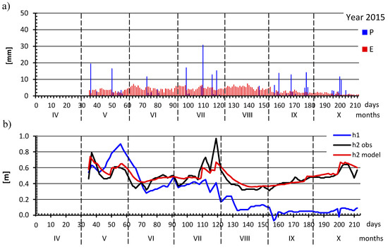
Figure 3.
(a) Precipitation P, Evapotranspiration E (b), measured and modeled groundwater tables (h2) for the calibration period of 2015 and observed water levels in the Mała river (h1).
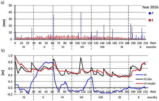
Figure 4.
(a) Precipitation P, Evapotranspiration E, (b) measured and modeled groundwater tables (h2) for the calibration period of 2016 and observed water levels in the Mała river (h1).
Validation was attempted on groundwater level data of 2017 (4 April to 31 October) utilizing the parameter values and lateral inflows qn determined in the previous stage. The resultant approximation error equaled 0.11 m, and the visual estimation of the groundwater level course pointed at a satisfactory model quality (Figure 5). Slightly different meteorological conditions and river water levels (h1) prevailed throughout the validation period (wet year of 2017) contrary to calibration one (dry years of 2015 and 2016—Table 1). This ensures, in particular, that the values of the parameters achieved for more dry conditions are also workable in a more wet, model validation period. Previous estimates of the parameters were available for the time constant T–that for a poorly permeable, decomposed fen soil becomes relatively long in comparison to mineral ones. Its value of 47 days was close to the one estimated in the previous studies-reaching 42.5 days [13] and referring to the same sub-irrigation system. The slightly lower value of was found for the analyzed fen peat soil as compared to literature data [23]. On the other hand, higher values of µ-specific yield were achieved (0.19) but in the proposed model it could be treated as an environmental, proxy parameter that may have a link with the average water table position on the plot (reference to Equations (3)–(7) and (10) in particular). For this reason, the value of µ may be used to explain areal water storage changes on the plot in general, not only within the soil profile. Basing on the above concept, the water balance for the needs of drainage -irrigation scheduling can be further developed for a plot or eventually for the whole system with the use of the proposed model.
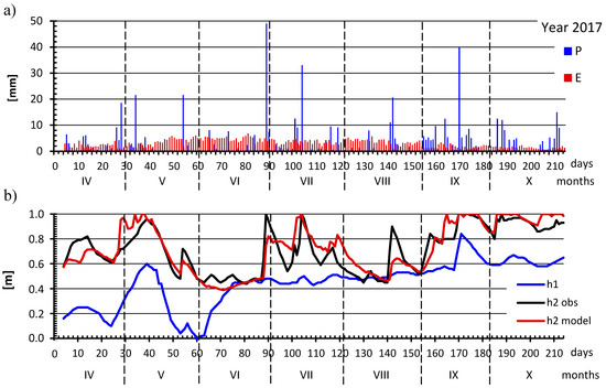
Figure 5.
(a) Precipitation P, evapotranspiration E, (b) measured and modeled groundwater tables (h2) for the validation period of 2017 and observed water levels in the Mała river (h1).
The analyzed organic (fen) soil was underlain by heavy clay leading to the assumption of the limited impact of the vertical leakance between the aquifers. This is consistent with the calibrated, relatively low value of the exchange parameter S = 3∙10−5 day−1 also suggested by the literature data [24].
With respect to the achieved parameter values, the model reflected the typical situation of the drainage-sub-irrigation plot in a lowland valley covered by fen soils. The characteristic feature is the poorly permeable base existing with the system, suggesting the model would explain groundwater tables course in ditch midspacing as driven by river water levels, precipitation and evapotranspiration, and also recharge from external sources, but not influenced by vertical flow exchange with the aquifer.
3.2. Lateral Inflows (qn)
The location of the analyzed subirrigation plot within the river valley may enhance the lateral inflow of groundwater from uplands, slopes—i.e., different neighboring recharge areas. Its’ rates are frequently subject to calibration since the aquifers or water-bearing units are found to be heterogeneous and some hydrogeological information may be missing. This pertains to the nature of hydraulic contact with adjacent areas, either recharging (qn–positive) or discharging (negative values of qn). This is the case that may be approached by the proposed model (qn = qi − qo) along with other issues to be addressed, such as hydraulic contacts with a river or stream or soil water retention temporal courses. Model calibration revealed the following, daily values of qn (Figure 6 and Figure 7).
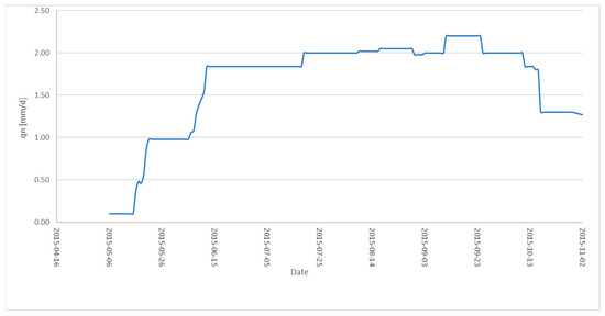
Figure 6.
Inflows qn calibrated for 2015.
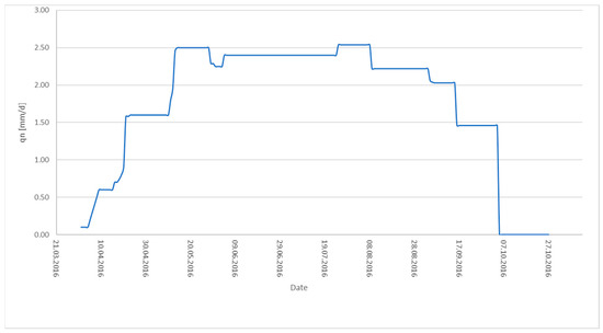
Figure 7.
Inflows qn calibrated for 2016.
Their courses were found to be similar for 2015 and 2016, and the daily averaged values (basing on both years) were used in the validation process on 2017 data to evidence if the model reproduced properly the groundwater level dynamics. In case of a more extensive data range available, 2017 would be also used for the calibration since it was estimated to be a wet year. It could offer better accuracy (smaller approximation error of the model validation than 0.11 m.) suppose the qn values were also calibrated for that year separately–for different hydrologic conditions. All in all, the approach to the calibration involved, at first, the optimization of the global parameter values [17,20] and then manual adjustment of the inflows qn. The resultant standard deviation of residual values (approximation error) reflected the choice of both main parameter values and daily qn rates.
The conceptualization of the lateral inflows involves a couple of cases from the viewpoint of model application. Their values may reflect the impact of other external or internal sources of water (e.g., irrigation, water intakes). Based on the above statement, they allow one to assume the river valley with lateral recharge, as considered herein. However, in a general sense, those inflows explain groundwater fluctuations in case of a lack of upward seepage (impermeable base) or probable, minor impact of river water levels (e.g., detached or disconnected streams). They may also compensate for water shortages either excess existing with the sub-irrigation system-the calibrated positive values for 2015 and 2016 stand for the required amount to come into storage throughout the vegetation season (negative values would suggest the excess be taken out of storage). Their course seems reasonable since both years were characterized as dry and undoubtedly additional inflows to the ditch system were required to maintain the groundwater table position. Nonetheless, this generates the potential for the future applications of the model to account for the impact of adjacent areas on water management practices.
4. Summary and Conclusions
Drainage–irrigation systems functioning has been described by a number of parameters, some of which have been approached conceptually. This pertains to proper mathematical models, having been developed for water movement in the soil taking into account all fluxes through groundwater table in a most common manner. The model proposed herein was conceptualized as the groundwater dynamics equation, soil moisture content equation to interpret transient porosity storage, and finally, the water balance equation that was only mentioned for future model development. This has been initially done in search of more simple, non-complex procedures for drainage–irrigation systems management with a range of measurable and interpretable parameters, which choice becomes specific and depends on the nature of the developed model. This is also the case of the proposed model–named Irrdrain which is dedicated, first of all, to groundwater level and soil moisture content estimation in ditch midspacing, pointing initially at the robustness of applied parameters and indexes.
At first, it can be concluded that a wide range of models has been dedicated to soil processes with some challenges remaining [1,2,4,6]. Models for drainage–irrigation practices estimation have still been important and efforts have been undertaken to devise a workable model with mainly physically- based parameters [9,10,12]. The procedure being developed herein was validated on groundwater level data set of two vegetation seasons showing a satisfactory match between the model and observations. This proves the establishment of a proper link between soil water leakage and the groundwater table of the saturated zone as assumed by the model structure. A flexible character of the modeling procedure was revealed with respect to the form of equations and parameters. The achievement is the existence of easily obtainable parameters, giving the base to develop operational drainage–irrigation scheduling model. This would lead to the more effective management of the water flows to individual plots and evidence for particular hydrological measures.
Generally, the reliability of the proposed procedure is initially proven, since it would require sensitivity analysis and also alternative calibration attempts on precise soil water content dataset.
The model offered the potential for ditch midspacing groundwater level estimates as influenced by river stages and specifically by inflow from adjacent areas. After their successful calibration it would become the base for a reliable, future tool for controlled water table strategies, but also to evaluate hydrological functions, surface water-groundwater interactions, and necessary flow alterations in valley sub-irrigation systems.
Author Contributions
Conceptualization, A.B. and E.K.; methodology, E.K.; validation, R.O., E.K., and J.U.; formal analysis, A.B.; investigation, A.B., E.K., and R.O.; resources, J.J.; writing—original draft preparation, A.B.; writing—review and editing, R.O. and J.J.; visualization, J.U.; supervision, E.K.; project administration, E.K., A.B., R.O., and J.U.; funding acquisition, E.K. All authors have read and agreed to the published version of the manuscript.
Funding
This research was funded by the Polish National Centre for Research and Development grant number BIO-STRATEG3/347837/11/NCBR/2017.
Acknowledgments
This study was done within the project “Technological innovations and system of monitoring, forecasting and planning of irrigation and drainage for precise water management on the scale of drainage/irrigation system (INOMEL)” under the BIO-STRATEG3 program, funded by the Polish National Centre for Research and Development. Contract number BIO-STRATEG3/347837/11/NCBR/2017.
Conflicts of Interest
The authors declare no conflict of interest.
References
- Van Keulen, H.; Van Beek, C.G. Water movement in layered soils—A simulation model. Neth. J. Agric. Sci. 1971, 19, 138–153. [Google Scholar] [CrossRef]
- Wierenga, P.J.; De Wit, C.T. Simulation of heat transfer in soils. Soil Sci. Soc. Am. Proc. 1970, 34, 845–848. [Google Scholar] [CrossRef]
- Gerke, H.H.; van Genuchten, M.T. A dual-porosity model for simulating the preferential movement of water and solutes in structured porous-media. Water Resour. Res. 1993, 29, 305–319. [Google Scholar] [CrossRef]
- Van Veen, J.A.; Paul, E.A. Organic-carbon dynamics in grassland soils. 1. Background information and computer-simulation. Can. J. Soil Sci. 1981, 61, 185–201. [Google Scholar] [CrossRef]
- Cole, C.V.; Innis, G.S.; Stewart, J.W. Simulations of phosphorus cycling in semi arid grasslands. In Grassland Simulation Model; Innis, G.S., Ed.; Springer: New York, NY, USA, 1978; Volume 26, pp. 205–230. [Google Scholar] [CrossRef]
- Hunt, H.W.; Wall, D.H. Modelling the effects of loss of soil biodiversity on ecosystem function. Glob. Chang. Biol. 2002, 8, 33–50. [Google Scholar] [CrossRef]
- Hopmans, J.W.; Bristow, K.L. Current Capabilities and Future Needs of Root Water and Nutrient Uptake Modeling. Adv. Agron. 2002, 77, 103–183. [Google Scholar]
- Javaux, M.V.; Couvreur, J.; Borght, V.; Vereecken, H. Root water uptake: From three-dimensional biophysical processes to macroscopic modeling approaches. Vadose Zone J. 2013, 12. [Google Scholar] [CrossRef]
- Schnepf, A.; Roose, T.; Schweiger, P. Impact of growth and uptake patterns of arbuscular mycorrhizal fungi on plant phosphorus uptake—A modelling study. Plant. Soil 2008, 312, 85–99. [Google Scholar] [CrossRef]
- Leitner, D.; Klepsch, S.; Ptashnyk, M.; Marchant, A.; Kirk, G.J.; Schnepf, A.; Roose, T. A dynamic model of nutrient uptake by root hairs. New Phytol. 2010, 185, 792–802. [Google Scholar] [CrossRef]
- Kaca, E. Modeling of Subirrigation; Wydawnictwo IMUZ: Falenty, Poland, 1999; p. 115, (In Polish with English Summary). [Google Scholar]
- Vogel, H.J.; Roth, K. Moving through scales of flow and transport in soil. J. Hydrol. 2003, 272, 95–106. [Google Scholar] [CrossRef]
- Brandyk, T.; Leeds-Harrison, P.; Skapski, K. A simple flow resistance model for the management of drainage/sub-irrigation systems. Agric. Water Manag. 1992, 21, 67–77. [Google Scholar] [CrossRef]
- IUSS Working Group WRB. World Reference Base for Soil Resources 2014, Update 2015: International Soil Classification System for Naming Soils and Creating Legends for Soil Maps; Fao: Rome, Italy, 2015. [Google Scholar]
- Gurley Kahn, K.; Ge, S.; Saul Caine, J.; Manning, A. Characterization of the shallow groundwater system in an alpine watershed: Handcart Gulch, Colorado, USA. Hydrogeol. J. 2008, 16, 103–121. [Google Scholar] [CrossRef]
- Eijkelkamp. Laboratory Permeameters. User Manual. 2020 [WWW Document]. Available online: https://en.eijkelkamp.com/products/laboratory-equipment/ (accessed on 17 November 2020).
- Brandyk, A.; Kiczko, A.; Majewski, G.; Kleniewska, M.; Krukowski, M. Uncertainty of Derdorff’s soil moisture model based on continuous TDR measurements for sandy loam soil. J. Hydrol. Hydromech. 2016, 64, 23–29. [Google Scholar] [CrossRef]
- Łabędzki, L. Agricultural Droughts an Outline of Problems and Methods of Monitoring and Classification; Wydawnictwo IMUZ: Falenty, Poland, 2006; 107p, (In polish with English summary). [Google Scholar]
- Bąk, B.; Łabędzki, L. Assessing drought severity with the relative precipitation index (RPI) and the standardized precipitation index (SPI). J. Water Land Dev. 2002, 6, 29–49. [Google Scholar]
- Kalyanmoy, D. Optimization for Engineering Design; Prentice Hall: New Delhi, India, 1988. [Google Scholar]
- Calderon-Palma, H.; Bentley, L. A regional scale groundwater flow model for the Leon- Chinandega aquifer, Nicaragua. Hydrogeol. J. 2007, 15, 1457–1472. [Google Scholar] [CrossRef]
- Copty, N.; Sarioglu, M.; Findikakis, A. Equivalent transmissivity of heterogeneous leaky aquifers for steady state radial flow. Water Resour. Res. 2006, 42, W04416. [Google Scholar] [CrossRef]
- Brandyk, T.; Szatylowicz, J.; Oleszczuk, R.; Gnatowski, T. Water-related physical attributes of organic soils. In Organic Soils and Peat Materials for Sustainable Agriculture, 1st ed.; Parent, L.E., Ilnicki, P., Eds.; CRC Press and International Peat Society: Boca Raton, FL, USA, 2002. [Google Scholar]
- Khadri, S.; Pande, C. Ground water flow modeling for calibrating steady state using MODFLOW software: A case study of Mahesh River basin, India. Modeling Earth Syst. Environ. 2016, 2, 39. [Google Scholar] [CrossRef]


Publisher’s Note: MDPI stays neutral with regard to jurisdictional claims in published maps and institutional affiliations. |
© 2020 by the authors. Licensee MDPI, Basel, Switzerland. This article is an open access article distributed under the terms and conditions of the Creative Commons Attribution (CC BY) license (http://creativecommons.org/licenses/by/4.0/).