A Novel Strategy for Optimal PSO Control Parameters Determination for PV Energy Systems

Abstract

This study introduces a novel strategy that can determine the optimal values of control parameters of a PSO. These optimal control parameters will be very valuable to all the online optimization problems where the convergence time and the failure convergence rate are vital concerns. The newly proposed strategy uses two nested PSO (NESTPSO) searching loops; the inner one contained the original objective function, and the outer one used the inner PSO as a fitness function. The control parameters and the swarm size acted as the optimization variables for the outer loop. These variables were optimized for the lowest premature convergence rate, the lowest number of iterations, and the lowest swarm size. The new proposed strategy can be used for all the swarm optimization techniques as well. The results showed the superiority of the proposed NESTPSO control parameter determination when compared with several state of the art PSO strategies.

1. Introduction

Swarm optimization techniques have displayed highly effective tracking of the optimal solutions in various applications. These techniques send searching agents to determine the values of fitness functions and use this information to move these agents toward the optimal value. The first metaheuristic technique was proposed by Tillman (1969) [1]. Particle swarm optimization (PSO) is one of the most popular metaheuristic optimization techniques of the last two decades, owing to its simplicity and reliability, with its usage increasing every day [2]. The PSO technique introduced by Kennedy and Eberhart (1995) [3] is inspired by the behavior of the flocks of fish, birds, swarms, and shoals searching for food, and it is used to determine the optimal solutions for multi-dimensional problems. This technique uses several particles to search for the optimal solution in the search space of the optimization problem. In the consecutive iterations (movements), the PSO collects the information gained from the particles to guide them in the next movement to the global optima. The new movement of each particle depends on the experience gained from the previous movements, the information gained from the best position of the particle itself (cognitive or self-experience), and the information gained from the global optimum (social experience). The confidence of capturing the global peak and the convergence speed are highly affected by the choice of PSO control parameters (acceleration parameters cl and c_g, and inertia weight ω) that are affected considerably by the fitness function. The equations governing the performance of the PSO technique are expressed as shown in (1) and (2) [4]. The acceleration parameters cl and cg are also called the self-confidence and the swarm-confidence parameters, respectively. Increasing the value of c_g affects the attraction of particles toward the best individual. Additionally, increasing the value of cl enhances the self-confidence search and vice versa. The inertia weight ω is used to enhance the stability of the particles, and its value affects the performance of the PSO searching behavior such that a high value of ω enhances the social search and reduces the cognitive search, and vice versa. The first usage of the ω in PSO was reported in [4]. The definitions of these symbols are listed in the list of symbols shown in the Abbreviations.

$$V_{i+1}^k=\omega V_i{}^k+c_l{r}_l^{}\left(L_{}^k-X_i{}^k\right)+c_g{r}_g^{}\left(G-X_i{}^k\right),$$

(1)

$$X_{i+1}^k=X_i{}^k+V_{i+1}^k,$$

(2)

The performance of the PSO in its journey to capture the global optima is governed by the values of ω, c_l, and c_g. While evaluating the performance of the PSO, the premature convergence rate (PCR) and the speed of convergence are the major concerns. The PCR is used to measure the number of times the PSO failed to capture the global optima or was trapped in one of the local peaks divided by the total number of attempts, which can be obtained from (3). The convergence time consumed to reach the final convergence is proportional to the number of iterations N, multiplied by SS, as shown in Equation (4). The factor N_SS is used to count the number of attempts to hit the fitness function, through the optimization process, which can represent the convergence time.

$$PCR=N_{PCR}/N_{av}\ast 100,$$

(3)

where N_PCR is the number of occurrences of premature convergence and N_av is the total number of experimental occurrences.

N_SS = N * SS,

(4)

The purpose of any strategy used to modify the performance of the PSO is to reduce the two factors PCR and N_SS. These two factors are such that for a low PCR, a large N_SS is expected and vice versa. These two factors are vital to be minimized, especially in online applications where the confidence and the convergence time are crucial issues and the focus of this study. Many strategies have been suggested in the literature to minimize these two factors. There are two major modification strategies, the first one is the mutation of the particles’ positions [5,6,7] and the second one is the tuning of PSO control parameters (ω, c_l, and c_g) [8,9,10,11,12,13,14,15]. Some researchers used these two improvement strategies together to improve the performance of PSO [16,17]. The mutation strategy of the PSO changes the position of the particles based on many stochastic strategies without changing the velocity of the particles. Adjusting the next movement helps the particles to escape from convergence at one of the local optimal solutions. An adaptive mutation strategy was introduced in [18] to adjust the particle movement distance automatically. A Gaussian mutation algorithm (GPSO) was introduced in [6] that uses neighbor heuristics and the Gaussian cloud learning PSO algorithm. Cauchy mutation strategy uses a scaling factor on the Cauchy mutation to control the distance the particle moves [7]. A detailed review with the evaluation of the mutation strategies is introduced in [5]. The mutation strategies slightly improve the premature convergence rate; however, they increase the convergence time and add complexity to the PSO strategy. Therefore, they have not been discussed further in this study.

The second improvement in the PSO is achieved by fine-tuning the PSO control parameters ω, c_l, and c_g, which considerably improves the performance of the PSO without adding extra complexity to the conventional PSO technique. Numerous studies have introduced different strategies to estimate the best values of the PSO control parameters [8,9,10,11,12,13,14,15]. Most of these strategies include tuning these parameters to improve the performance of the PSO using the trial-and-error mechanism or using the empirical formulas. Few strategies have shown successful results in certain applications; however, they have failed in some other applications. Thus, there is a need for fine-tuning the PSO control parameters for different applications. Two strategies were used for this purpose, the first one depends on using fixed values of the PSO control parameters, which can be determined using the different strategies suggested in [8,9,10,11,12,13,14,15,19,20,21,22,23,24,25,26,27,28,29], the other strategy is called the online strategy, where the values of PSO control parameters are changing during the execution of the code. Fixed control parameters are fixed during the entire iterations of the searching space. Therefore, these PSO control parameters should be known before running the PSO code to search for the optimal solution. Most of these studies have used the recommended values of these parameters based on the previous studies or after fine-tuning these parameters to be more effective in a certain application. Some researchers introduced empirical formulas to assist in choosing the PSO control parameters [16,19]. Some studies introduced a mathematical derivation for obtaining the optimal values of the PSO parameters [20,21], considering the effects of these parameters on the behavior of the PSO. Kennedy et al. [3] introduced the first study on the effect of the PSO control parameters values on its searching performance; they recommended the values of c_g, c_l, and ω as 2, 2, and 1, respectively. Another study discussed the effect of ω and other PSO parameters, c_g and c_l, on the performance of PSO using the trial-and-error mechanism [30] and concluded that it is beneficial to use the linearly decreasing inertia weight, as will be discussed later. Eberhart [20] introduced a modified strategy considering the relation between the PSO control parameters called the constriction factor, as expressed in (5) and (6). This strategy introduced the values of control parameters that may work well with a certain application; however, they were not suitable for other applications, as shown in the experimental results of this study.

$$\omega =\frac{2}{\left|2-(\varphi )-\sqrt{{\varphi }^2-4\varphi }\right|},$$

(5)

$$\mathrm{where},\varphi =\frac{c_g+c_l}{\omega }>4,$$

(6)

Clerck [9] concluded that the most suitable value of ϕ was 4.1, which showed many positive results. Therefore, from (5) and (6), ω = 0.729, and the author assumed c_g = c_l = 1.49445 [9]. Additionally, an empirical formula was introduced in [16] to examine the performance of the PSO search with the varying PSO control parameters. The main inference from this study was that the balance between the acceleration parameters, c_g and c_l, does influence the regions of the parameter space that leads to approximately optimal performance. The relation between c_g, c_l, and ω is defined in (5). Additionally, this strategy introduced a relation between ω and (c_g + c_l); however, the deterministic values of these parameters that can fit with all optimization problems were not introduced. It was checked with the optimal values of control parameters that show the highest performance; however, it was not compatible with this condition, as shown in [16].

$$c_g+c_l>\frac{24({\omega }^2-1)}{5\omega -7},$$

(7)

Additional empirical formulas that can assist in determining or introducing the boundary values of the PSO control parameters were introduced in [10,17,22,23]. Additionally, all these empirical formulas were tested, and it was found that they might be suitable for a certain application, but not suitable for all optimization problems. The authors of [10] recommended the values ω = 0.715 and c_g = c_l = 1.7, and concluded that the most suitable values of the PSO control parameters depended on the experimental findings. Nevertheless, this strategy was tested, and it was found that it was not suitable for all the optimization problems, as shown in the results of this study. Most of the recommended and popular strategies estimating the control parameters [8,9,10,11,12,13,14,15,19,20,21,22,23,24,25,26,27,28,29] were tested with the final recommendations of this study. This study concludes that all these strategies may work well for a certain application; however, they will not work well in all the optimization problems.

Another strategy is the online strategy; it changes the values of the PSO parameters during the search progress to enhance the social search at the beginning of the search operation to capture the global best (GB) and not fall in one of the local best (LB). Additionally, it enhances the cognitive search to capture the GB accurately and with the least oscillations around it [31]. Most of the online PSO parameter variations were examined and compared in [32,33]. An online strategy can be subclassified into two types, namely, the dynamic strategies [30,34,35,36] and the adaptive strategies [32]. A dynamic strategy uses certain formulas to change the values of the PSO parameters with iterations. The dynamic strategy enhances the social search at the beginning of the iterations by increasing the values of the inertia weight parameter. Subsequently, it enhances the cognitive search by reducing the values of the inertia weight parameter with increasing the number of iterations. Meanwhile, the adaptive strategy adapts the PSO control parameters, depending on the progress achieved during the search based on the online results from the search progress. Reference [37] introduced a formula for dynamic variation equations for the acceleration parameters besides the inertia weight. This strategy requires the introduction of optimal dynamic equations for PSO control parameters.

Based on the previous discussion, it was concluded that the performance of PSO techniques is highly affected by the values of PSO control parameters, especially in online applications where the confidence of capturing the GB and the convergence time are the crucial factors. The previous strategies used recommended or tuned values of PSO control parameters.

The proposed strategy introduced in this study focuses on the determination of the optimal fixed control parameters, and therefore, the dynamic variation in the PSO control parameters has not be further discussed. This is a pioneer study that has introduced a strategy to determine the optimal PSO control parameters in the metaheuristic techniques for minimum PCR and the shortest convergence time that suits all the applications. This new proposed strategy uses two nested PSO loops and is called NESTPSO. The inner one is to get the optimal solution of the fitness function and the outer one optimizes the PSO control parameters of the inner loop to get the lowest PCR and N_SS for the inner loop. Thus, the control parameters of the inner PSO are used as optimization variables in the outer PSO loop. The fitness function to be minimized in the outer loop is a multiobjective function containing the PCR and the N_SS of the inner PSO loop. The stunning results obtained from using the NESTPSO in the optimization of many benchmark functions with different levels of complexity and the real-world application show a substantial reduction in convergence time and PCR compared to 10 state-of-the-art strategies. This improvement gained from NESTPSO allows the use of the PSO in the online applications that need very fast and reliable convergence, such as the maximum power point tracker (MPPT) of the PV systems. Moreover, NESTPSO can determine the optimal swarm size for optimal optimization performance. The author has ambition in this strategy to open a new way of optimally determining the control parameters of all swarm optimization techniques in the engineering optimization field.

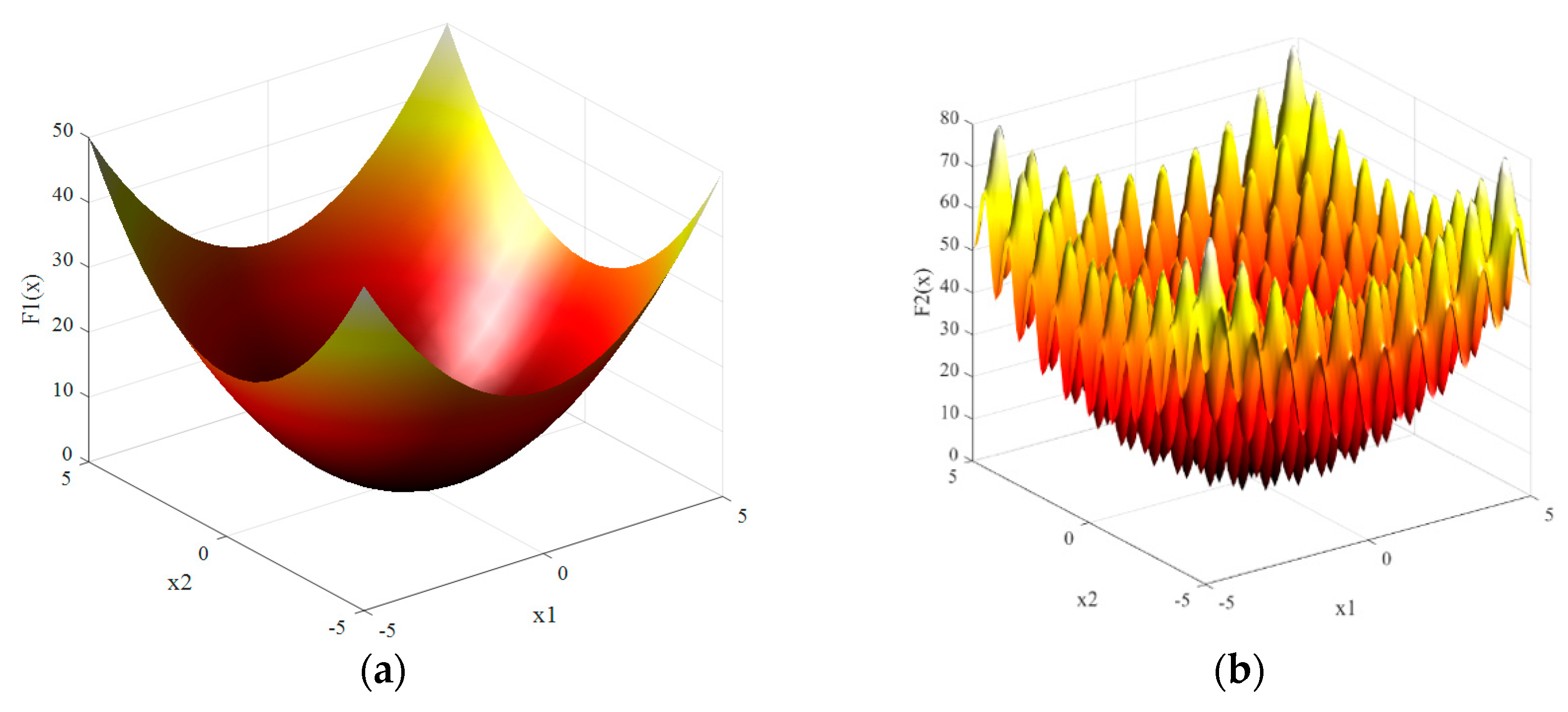
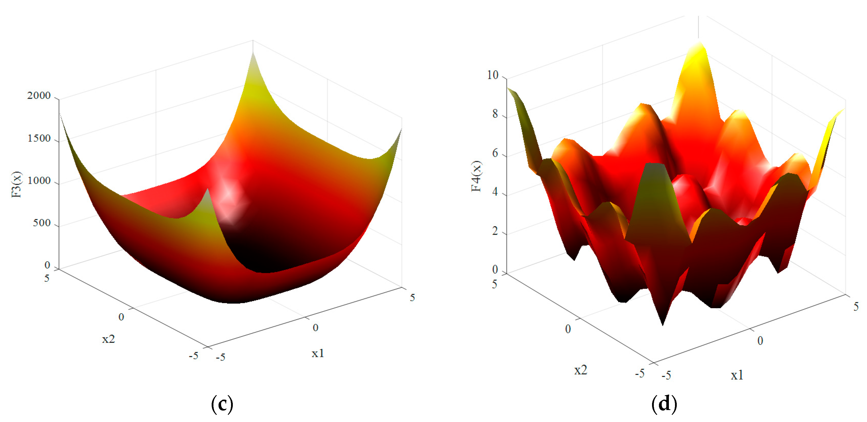
The rest of the paper is designed thus: Section 2 explains the proposed strategy and its logic. Section 3 introduces the experimental results of the proposed strategy compared to the state-of-the-art strategies with four benchmark mathematical functions. Section 4 shows the application of NESTPSO as an MPPT of PV energy system compared to state-of-the-art strategies. Section 5 shows the conclusions of the study and introduced future work.

2. Proposed Strategy

The concept proposed in this study can be applied to all the PSO parameter estimation strategies, where it can be used with fixed PSO parameters, dynamic PSO, and adaptive PSO parameter variations. Moreover, this strategy can be used to determine the optimal parameters for all metaheuristic techniques. The proposed strategy for PSO control parameter (ω, c_l, and c_g) determination is called the nested PSO (NESTPSO). The term nested PSO has been introduced in many researches [38,39,40,41,42,43,44] to handle certain functions. However, it has been used in this paper to determine the control parameters of PSO or any other metaheuristic techniques. All the previous studies depended on non-autonomous strategies to estimate the control parameters of the PSO. Two nested PSO searching loops are used, where the inner PSO loop contains the fitness function required to be optimized. The outer PSO loop uses the inner PSO as a fitness function to minimize the PCR and N_SS. The PSO parameters of the inner loop (ω_i, c_li, and c_gi) and swarm size (SS_i) are used as the variables to be optimized in the outer loop. 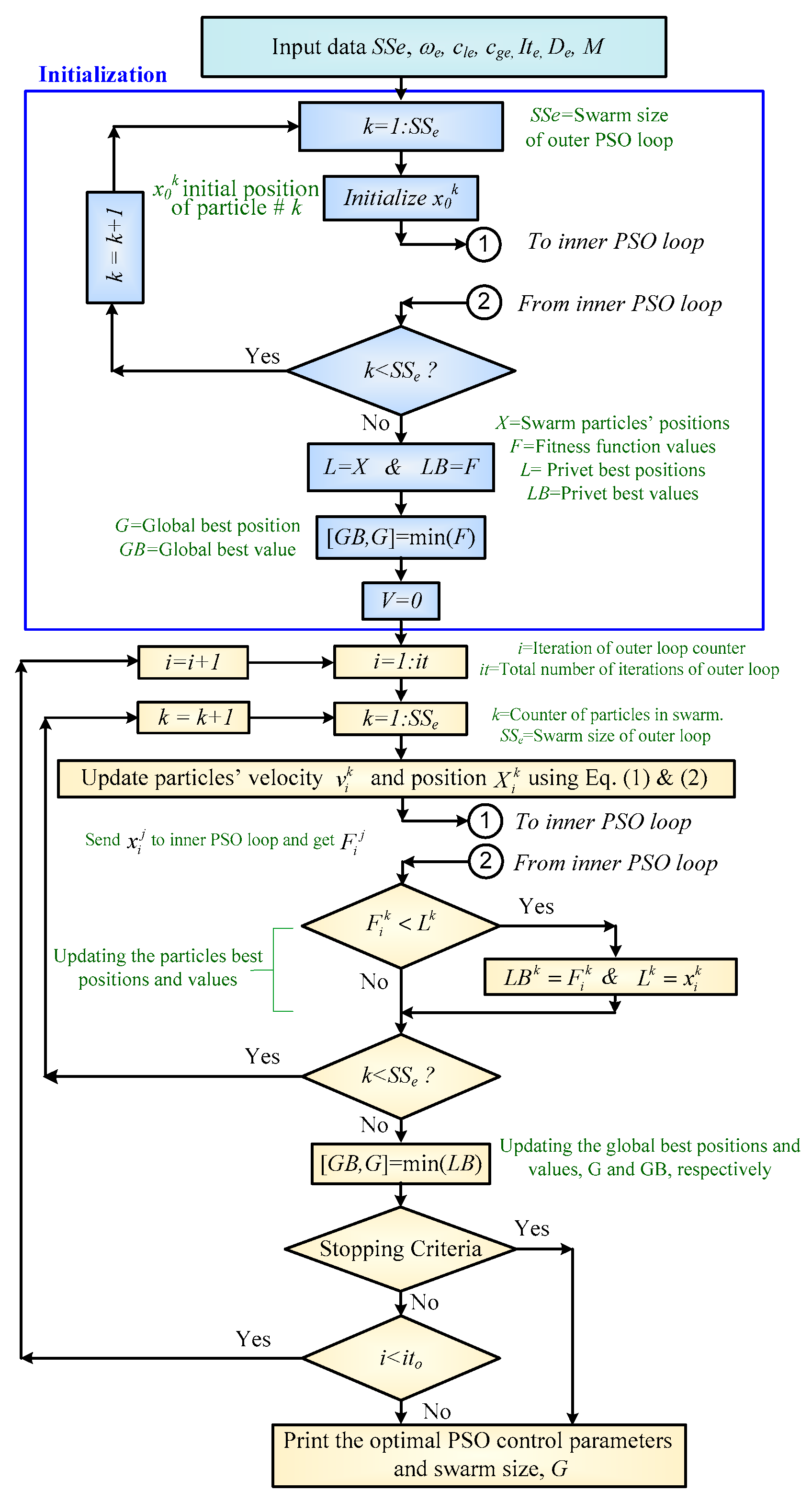The outer PSO loop control parameters’ values are given in [20], where ω_e = 0.729, and c_le = c_ge = 1.49445. The swarm size of the outer loop is chosen to be equal to 50 particles. 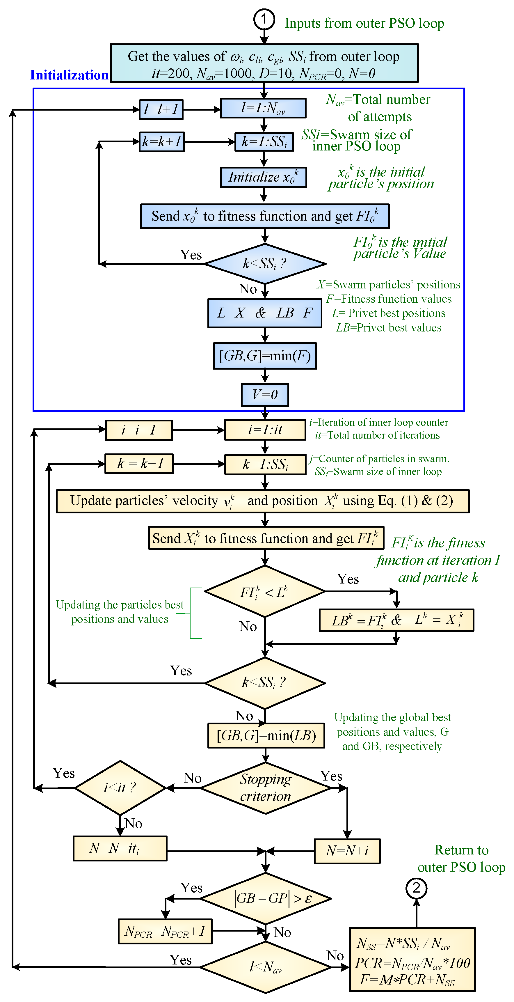A block diagram showing the logic used to determine the optimal values of control parameters in the NESTPSO is shown in Figure 1 and Figure 2 for the outer and inner PSO loops, respectively. At the beginning of the iteration process, the outer PSO loop initiated random values for the control parameters and the swarm size of the inner PSO loop. These values are applied to the inner PSO loop to minimize the benchmark mathematical functions used in this study. To avoid the effect of the random nature inherent in the inner PSO loop, the function is minimized for a certain number of iterations, N_av, to obtain the average results. After performing N_av iterations for the inner loop, the times the inner loop is trapped in the local optima are counted as a variable N_PCR and the PCR is determined from (3). The number of average iterations in the inner loop, N_i, is determined and used to determine the average value of N_SS, as shown in (4). The multi-objective function is determined in terms of PCR and N_SS, as shown in (8), to get the optimal PSO parameters of the inner function for minimum PCR and N_SS. These two parameters displayed opposite performance, which means to get minimum PCR, N_SS had to be increased, and vice versa. Therefore, the multi-objective function shown in (8) is introduced to achieve a trade-off between these two factors.

F = M*PCR + N_SS,

(8)

where M is a weighting value to be multiplied with the PCR to express the importance of PCR compared to the N_SS. A detailed study to determine the value of M is shown in the experimental results.

Minimizing the objective function, F in the outer PSO loop guaranteed optimal PSO control parameters and swarm size of the inner loop for minimum PCR and N_SS. The optimal values of the control parameters of the inner loop are obtained as the optimal solutions for the outer loop. The detailed pseudo-code explaining this new strategy (NESTPSO) for obtaining the optimal values of the PSO control parameters is shown in Figure 3 and Figure 4 for the outer and inner loops, respectively. It is clear that the control parameters and the swarm size of the inner PSO loop are fed from the outer PSO loop as optimized variables. The concept of using the NESTPSO in the determination of the parameters of metaheuristic techniques has not been reported in the literature before. The proposed strategy can be used as an on-shelf optimal parameter estimation for any metaheuristic technique, which will assist researchers and designers to use their proposed metaheuristic techniques with optimal performance. This new strategy ensures fast and reliable convergence for any fitness function used with any metaheuristic technique. The proposed strategy will open a new way for the optimal determination of metaheuristic techniques parameters estimation and other applications.

3. Experimental Results and Discussion

The experimental work of the proposed strategy, NESTPSO, is performed for four benchmark mathematical functions, as shown in (9)–(12). The results obtained from NESTPSO are compared to 10 fixed control parameters in the PSO strategies [8,9,10,11,12,13,14,15].

3.1. Benchmark Mathematical Functions

The four selected benchmark mathematical functions have zero minimum value. These benchmark functions are shown in the following Equations (9)–(12). The order of these benchmark functions is set at D = 10. These function are drawn in Figure 5 for two dimensional order (D = 2).

The first benchmark function, the sphere function is shown in the following equation:

$$F_1\left(x\right)={\displaystyle \sum _{i=1}^D{x}_i^2},$$

(9)

where x = [X₁, X₂, …, X_D], and D denotes the variables that determines the order of fitness function.

The second benchmark function is the generalized Rastrigrin function, which is described by the following equation:

$$F_2\left(x\right)={\displaystyle \sum _{i=1}^D\left(x_i^2-10\cos \left(2\pi x_i\right)+10\right)},$$

(10)

The third benchmark function is the De Jong function, which is described by the following equation:

$$F_3\left(x\right)={\displaystyle \sum _{i=1}^{D}i{x}_i^4}$$

(11)

The fourth benchmark function is the Alpine function, which is described by the following equation:

$$F_4\left(x\right)={\displaystyle \sum _{i=1}^D\left|x_i^{}\sin x_i+0.1x_i\right|}$$

(12)

3.2. Stopping Criterion

The stopping criterion is a condition used to terminate the execution of the code when the convergence occurred with a certain value. Many stopping criteria are introduced in the literature [45] to decide to stop the execution of the code, such as:

• Generation Number: The execution of the code is to stop when the iteration number equals the predefined number of iterations.
• Best Fitness Threshold: This condition stops the execution of the code when the value of the fitness function reached predefined value.
• Population Convergence: This condition stops the execution of the code when the difference between the maximum and minimum values of all particles’ position in the population is less than the predefined tolerance. This idea also can be achieved by using the standard deviation of the particle position of private best is less than predefined tolerance, which has been used in this study for the first time based on the knowledge of the author of this research.
• Fitness Convergence: This stops the iteration when the difference between the maximum and minimum values of objective function during one iteration is less than the predefined tolerance.

In this study, the generation number and population convergence stopping criteria have been used to stop the execution of the logic in the inner and outer loops. Regarding the generation number, the stopping criterion has been used in the inner and outer loops by setting the maximum number of iterations to 200 iterations for inner and outer PSO loops. Regarding the population convergence of the inner loop, it is assumed that the complete convergence occurs when the maximum value of standard deviation (std) for all variables’ values of private particles’ best positions is lower than the predefined tolerance value, ε. The value of ε is chosen here by 0.001, as shown in the following Equation (13). This condition ensures that all the particles are concentrated near to each other, and the standard deviation of their position value is lower than 0.001. This criterion will reduce the convergences time, but it will not highly affect the final results. The value of the predefined tolerance ε is depending on the values of the optimal solutions of variables of the fitness function, which needs a careful selection of ε.

Max(std(P_best(1:SS_i))) ≤ ε

(13)

where P_best(i) is the values of particle best positions of the inner loop, and ε is the acceptable values of the standard deviation of the particle best positions.

The above criteria used in the inner PSO loop will not work with the outer one, because the variables in the outer one are composed of different values of PSO control parameters ω, c_l, c_g, and SS. The fitness convergence stopping criterion is used to stop the outer PSO loop. This is accomplished by stopping the iterations of the outer PSO loop when the difference between the maximum and minimum values of the fitness function during one iteration is less than 1*10⁻⁵. This value has been chosen empirically after studying the performance of the convergence of the outer loop.

3.3. Premature Convergence Rate Determination

The premature convergence occurred when the particles of PSO are all trapped in one of the local optima to the end of the convergence iteration. It is not easy to deduce a generalized formula to be used to judge if the GB is the right global optima (theoretical optima), GO, or is one of the local optima, LO. To have a fair evaluation between all of these strategies, the absolute difference between the GB and GO is higher than 0.01 will be counted as premature convergence occurrence. The PSO searching strategy will be performed 1000 times to reduce the random nature inherent in the PSO technique. The PCR or sometimes called failure rate can be obtained from (3). Where the PCR equals the ratio of the total occurrence of premature convergence, N_PCR divided by the total number of searching occurrences (N_av), as shown in Equation (3). This value used to judge may be varied from one fitness function to another, but this value performed very well in all the benchmark functions (9)–(12) as well as the MPPT of the PV system.

The boundaries for the inner loop variables are set −5 to 5 for all benchmark functions understudy. Regarding the variables of the outer PSO loop that will be used as input to the inner PSO loop, the boundaries of these PSO control parameters (c_g, c_l, and ω) are set in between −5 and +5; meanwhile, the swarm size boundary is selected between 2 to 100.

3.4. Selecting of Multi-Objective Function Weighting Value

Two main studies are introduced here in this paper. The first one is introduced to show the variations of PCR and N_SS for different values of objective function weight parameter, M, for the four benchmark functions under study. The second one is introduced to compare the results obtained from NESTPSO with the recommended values of control parameters introduced in the literature [8,9,10,11,12,13,14,15,19,20,21,22,23,24,25,26,27,28,29].

The objective of the first study is introduced to select the most suitable value of M to achieve the lowest acceptable value of PCR and the lowest number of hitting the fitness function N_SS. As discussed above, the experiment of the benchmark mathematical functions is performed 1000 times to overcome the random nature inherent in the PSO technique. The variations in the control parameters of the inner loop (ω_i, c_li, and c_gi), PCR, and N_SS with M are shown in Figure 6, Figure 7, Figure 8, Figure 9, Figure 10, Figure 11, Figure 12 and Figure 13 for the Sphere, the Rastrigrin, the De Jong, and the Alpine benchmark functions, respectively. The results shown in Figure 6, Figure 7, Figure 8, Figure 9, Figure 10, Figure 11, Figure 12 and Figure 13 have been tabulated in

Table 1. Variation of m with the performance parameters of the inner PSO loop for the sphere function.

M	ωi	cli	cgi	SSi	PCR	Ni	NSS
70	0.8151	0.0048	0.8374	32	7.3400	94.01	3004
90	0.8216	0.0140	0.803	36	4.5000	92.83	3342
100	0.825	0.0187	0.784	38	3.2800	92.53	3516
110	0.8274	0.0232	0.7666	39	2.8500	91.95	3586
130	0.8329	0.031	0.7359	40	2.1800	91.60	3664
150	0.8386	0.0386	0.7053	44	1.2600	91.95	4046
170	0.8437	0.0449	0.6792	44	1.1300	93.34	4107
190	0.8484	0.0506	0.6538	44	0.9800	94.59	4162
200	0.8509	0.0534	0.642	44	0.9750	95.09	4184
210	0.853	0.0556	0.6324	44	0.9500	95.77	4214
300	0.8706	0.0697	0.5725	44	0.7400	104.89	4615
400	0.8839	0.0677	0.544	44	0.5000	111.89	4923
500	0.8905	0.05	0.5500	45	0.4000	116.71	5252

,

Table 2. Variation of M with the performance parameters of the inner PSO loop for the Rastrigrin function.

M	ωl	cli	cgi	SSi	PCR	Ni	NSS
30	0.7238	0.4824	0.4396	21	13.3	85.81	1805
40	0.7279	0.4867	0.4334	22	10.7	81.85	1862
50	0.7318	0.4909	0.424	22	9.5	87.47	1918
60	0.7355	0.495	0.42	23	8.2	89.5	1972
70	0.739	0.499	0.4173	24	6.4	81.94	2025
80	0.7424	0.5029	0.4142	24	5.5	81.464	2077
90	0.7455	0.5068	0.4133	25	4.5	90.83	2127
100	0.7485	0.5106	0.4126	25	4.1	87.34	2175
200	0.77	0.5448	0.4071	26	1.8	103.19	2586
300	0.7795	0.5717	0.409	27	0.99	98.87	2857
400	0.7822	0.5913	0.4158	28	0.4	110.71	2989
500	0.7828	0.6037	0.42	28	0.31	105.79	3005

,

Table 3. Variation of M with the performance parameters of the inner PSO loop for the De Jong function.

M	ωl	cli	cgi	SSi	PCR	Ni	NSS
30	0.803	−0.0005	0.97	25	6.5059	73.04	1826
40	0.789	−0.0002	0.9588	27	5.4398	68.74	1856
50	0.7831	0.0003	0.9501	29	4.496	65.21	1891
70	0.7774	0.0036	0.945	33	2.9464	60.00	1980
90	0.778	0.012	0.945	38	1.7984	54.92	2087
110	0.7838	0.018	0.947	42	0.9936	52.62	2210
130	0.7927	0.0218	0.9563	48	0.4734	48.83	2344
150	0.805	0.0323	0.963	53	0.1791	46.91	2486
170	0.814	0.04	0.966	57	0.0522	46.18	2632
190	0.817	0.045	0.964	60	0.0341	46.25	2775
210	0.82	0.049	0.956	64	0.012	45.94	2940

and

Table 4. Variation of M with the performance parameters of the inner PSO loop for the Alpine function.

M	ω	cli	cgi	SSi	PCR	Ni	NSS
70	0.7934	−0.0013	1.0005	32	12.4200	107.25	3432
100	0.7940	−0.0014	0.7961	38	10.1600	100.71	3827
130	0.7950	−0.0016	0.7229	42	9.1800	98.90	4154
160	0.8004	−0.005	0.6762	45	7.1700	103.11	4640
190	0.8113	−0.0107	0.6583	47	4.3300	113.62	5340
220	0.8248	−0.0132	0.6115	48	2.9500	124.77	5989
250	0.8585	−0.0154	0.5761	50	0.9200	164.30	8215
280	0.8800	−0.017	0.5664	52	0.4500	199.00	10,348

to display the information accurately and to simplify the comparison of these results. The detailed results of each benchmark function are shown in the following sections:

3.4.1. Multi-Objective Weighting Value for the Sphere Benchmark Function

The variation of M, with the control parameters of the inner loop (ω_i, cl_i, and c_gi), PCR, and N_SS are shown in Figure 6 and Table 1. The objective of this section is to determine the optimal value of M shown in Equation (8). It is clear from Figure 6 and Table 1 that the maximum value of PCR is 7.34 at M = 70. However, this value is lower than the best value obtained from the state-of-the-art strategies [8,9,10,11,12,13,14,15], as shown in

Table 5. Fixed control parameters strategies compared to the NESTPSO.

	Parameter	ωl	cli	cgi	SSi	F1, D = 10		F2, D = 10		F3, D = 10,		F4, D = 10
Strategy						NSS	PCR	NSS	PCR	NSS	PCR	NSS	PCR
S1 [8]		0.7298	1.4962	1.49618	50	6962	10.87	6868	0.40	3981	2.60	7452	16.64
S2 [9]		0.729	1.4945	1.4945		6932	11.11	7053	0.40	4022	2.60	7392	16.18
S3 [10]		0.715	1.7	1.7		8073	13.49	8330	0.60	4765	2.60	8228	20.63
S4 [12]		0.729	2.05	2.05		10,936	25.06	11,625	2.60	6989	9.00	10,126	32.37
S5 [11]		0.729	2.0412	0.9477		6190	8.63	6349	0.60	3707	2.40	7148	13.68
S6 [12]		0.724	1.468	1.468		6535	11.65	6664	0.60	4056	3.00	7068	17.55
S7 [13]		0.72	1.108	1.108		4511	14.78	4759	0.20	2979	2.80	5161	18.80
S8 [14]		0.42	1.55	1.55		1682	95.34	2159	42.40	1707	62.20	1702	95.54
S9 [15]		0.5	1.9	1.9		3232	69.26	4054	10.60	3044	29.40	3620	71.01
S10 [15]		0.6	1.8	1.8		4815	38.90	5590	3.20	3951	10.20	5397	42.92
NESTPSO	Case 1(M = 90)	0.8216	0.014	0.803	36	3342	4.50
	Case 2(M = 190)	0.8484	0.0506	0.6538	44	4162	0.98
	Case 3 (M = 90)	0.7455	0.5068	0.4133	25			2127	4.500
	Case 4 (M = 300)	0.7795	0.5717	0.409	27			2857	0.99
	Case 5 (M = 50)	0.7831	0.0003	0.9501	29					1891	4.496
	Case 6 (M = 110)	0.7838	0.018	0.947	42					2210	0.994
	Case 7 (M = 190)	0.8113	−0.0107	0.6583	47							5340	4.33
	Case 8 (M = 250)	0.8585	−0.0154	0.5761	50							8215	0.92

. Additionally, it is clear that the value of M is inversely proportional to the PCR and directly proportional to the N_SS in the lower values of M; meanwhile, it shows a saturated relation with the higher values of M. The variation of SS_i, N_i, and N_SS with the value of PCR is shown in Figure 7. For best operating performance, the PSO should have the minimum value of PCR and N_SS. Here the PCR is inversely proportional to M, and N_SS is directly proportional to M. Therefore, a trade-off between these two values is required. The value of M is selected based on the acceptable lowest value of PCR, where, if PCR <= 5% (Case 1) is the acceptable value, the selected value of M = 90, and the values of ω_i, c_li, c_gi, SS_i, PCR, and N_SS are 0.8216, 0.0140, 0.803, 36, 4.5%, and 3342, respectively, as shown in Figure 6, Figure 7, and Table 1. Meanwhile, if PCR <=1% (Case 2) is the acceptable value, the selected value of M is equal to 190; the values of ω_i, c_li, c_gi, SS_i, PCR, and N_SS are 0.8484, 0.0506, 0.6538, 44, 0.98%, and 4162, respectively. These two cases are further compared to the state-of-the-art strategies [8,9,10,11,12,13,14,15] to show the superiority of NESTPSO. The difference between these two cases is that Case 2 required an additional 820 hitting the fitness function to reduce the PCR from 4.5% to 0.98%.

3.4.2. Multi-Objective Weighting Value for the Generalized Rastrigrin Function

The experimental work for the generalized Rastrigrin benchmark function is performed similarly to the Sphere function. The variation of M with the control parameters of the inner loop (ω_i, c_li, and c_gi), PCR, and N_SS are shown in Figure 8 and Table 2. It is clear from this figure that the value of M is inversely proportional to PCR and directly proportional to N_SS in the lower values of M; however, it saturates after M increases. The maximum value of PCR is 13.3% at M = 30. The value of M is selected based on the acceptable value of PCR, where if PCR <= 5% (Case 3) is the acceptable value, the selected value of M = 90, as shown in Table 2 and Figure 8. The values of ω_i, c_li, c_gi, SS_i, PCR, and N_SS are 0.7455, 0.5068, 0.4133, 25, 4.5%, and 2127, respectively, as shown in Table 5. If the acceptable value of PCR <= 1% (Case 4), the value of M = 300 is selected from Figure 9 and Table 2; the values of ω_i, c_li, c_gi, SS_i, PCR, and N_SS are 0.7795, 0.5717, 0.409, 0.99%, and 2857, respectively. These two cases are further compared to the state-of-the-art strategies [8,9,10,11,12,13,14,15] to show the superiority of the NESTPSO strategy. The difference between these two cases is that Case 4 required an extra 730 hitting the fitness function to reduce the PCR from 4.5% to 0.99%. The variation in SS_i, N_i, and N_SS with PCR for the Rastrigrin is shown in Figure 9.

3.4.3. Multi-Objective Weighting Value for the De Jong Benchmark Function

The experimental work for the De Jong benchmark function is performed in the beginning to determine the weight of the multi-objective function, M. The variation in M with the control parameters of the inner loop (ω_i, c_li, and c_gi), PCR, and N_SS are shown in Figure 10 and Table 3. It is clear from this figure that the maximum value of PCR is 6.5059% at M = 30. The value of PCR reduces swiftly with variation in M compared to the other two benchmark functions. The value of M is selected based on the lowest value of PCR, where, if PCR <= 5% (Case 5) is the acceptable value, the selected value of M = 50; values of ω_i, c_li, c_gi, SS_i, PCR, and N_SS are 0.783, 0.003, 0.9501, 29, 4.496%, and 1891, respectively. If PCR <= 1% (Case 6) is the acceptable value, the selected value of M = 110; values of ω_i, c_li, c_gi, SS_i, PCR, and N_SS are 0.7838, 0.018, 0947, 42, 0.9936%, and 2210, respectively. These two cases are further compared to the state-of-the-art strategies to show the superiority of NESTPSO. The difference between these two cases is that Case 6 required an extra 319 hitting the fitness function to reduce the PCR from 4.496% to 0.9936%. The results of this experiment are shown in Table 3. Negative values of c_li are observed for the first time in the literature. Figure 11 shows the variation in SS_i, N_i, and N_SS along with PCR.

3.4.4. Multi-Objective Weighting Value for the Alpine Benchmark Function

The experimental work for the Alpine Benchmark function is performed to determine the weight of the multi-objective function, M. The variation of the control parameters of the inner loop (ω_i, c_li, and c_gi), PCR, and N_SS, along with M are shown in Figure 12, Figure 13, and Table 4. It is clear from the figure that the value of M is inversely proportional to PCR and directly proportional to N_SS in the lower values of M; however, it saturates after M increases. It is clear that the maximum value of PCR is 12.42 at M = 70. This value is lower than all the state-of-the-art strategies. The value of M can be selected based on the lowest value of PCR, where if PCR <= 5% (Case 7) is the acceptable value, the selected value of M = 190; the values of ω_i, c_li, c_gi, SS_i, PCR, and N_SS are 0.8113, −0.0107, 0.6583, 47%, and 5340, respectively. If the acceptable value of PCR <= 1% (Case 8), the selected value of M = 250; values of ω_i, c_li, c_gi, SS_i, PCR, and N_SS are 0.8585, −0.0154, 0.5761, 50, 0.92%, and 8215, respectively. These two cases are further compared to the state-of-the-art strategies to show the superiority of NESTPSO. The difference between these two cases is that Case 8 needs an extra 2875 hitting the fitness function to reduce the PCR from 4.33% to 0.92%. This implies that Case 7 is faster than Case 8, but with a higher PCR (failure rate).

3.5. Comparison of NESTPSO to State-of-the-Art PSO Strategies

After studying the performance of the NESTPSO with the variation of M in the previous section, two values of M are selected for further study and comparison in each benchmark function under study. The selection of M depends on the allowed PCR, as has been discussed. The PSO control parameters of state-of-the-art strategies have been used to determine the PCR and the N_SS, to be compared to the values obtained in Cases 1–8, as discussed in Section 3.4. The following list is summarizing the different cases understudy:

• Case 1: sphere function and (M = 90)
• Case 2: sphere function and (M = 190)
• Case 3: Rastrigrin function and (M = 90)
• Case 4: Rastrigrin function and (M = 300)
• Case 5: De Jong function and (M = 50)
• Case 6: De Jong function and (M = 110)
• Case 7: Alpine function and (M = 190)
• Case 8: Alpine function and (M = 250)

The experimental work is performed 1000 times to achieve the average value that reduces the dependency of the output results on the stochastic nature of the PSO. Ten popular strategies are selected to be compared to the NESTPSO, as shown in Table 5 [8,9,10,11,12,13,14,15]. The results shown are the PCR and the N_SS. All state-of-the-art strategies [8,9,10,11,12,13,14,15] understudy had SS_i = 50; however, SS_i of the proposed strategy is the optimization variable determined from the NESTPSO. This implies that the proposed simulation program is optimizing the PSO control parameters and SS_i to achieve the lowest possible PCR and the lowest N_SS.

Increasing the value of M gives more weight to the PCR than the N_SS and vice versa. Therefore, it depends on the user’s requirements to give more weight to PCR or N_SS. The comparisons between the results obtained from the state-of-the-art strategies and the results obtained from the NESTPSO for the four benchmark mathematical functions are shown in the following subsections:

3.5.1. Comparison of NESTPSO with the State-of-the-Art PSO Strategies for the Sphere Function

The NESTPSO experimental work for the Sphere function is introduced in Table 1 and Figure 6 and Figure 7. Case 1 (PCR <= 5%, M = 90) and Case 2 (PCR <= 1%, M = 190) are selected to be further compared with the results obtained from the state-of-the-art strategies shown in Table 5.

The results of state-of-the-art strategies shown in Table 5 for the Sphere benchmark function show that the lowest PCR is 8.63% with N_SS = 6190 corresponding to strategy S5 [11]. This means that this strategy loses the global minimum by 8.63% of the total try for the Sphere function; meanwhile, it needs 6190 hits to the fitness function to converge. Meanwhile, the fastest convergence strategy is S8 [14] that needs 1682 hits to the fitness function to converge; however, it has the highest PCR at 95.34%, which indicates that it loses the GB by 95.34%, showing low-performance results. The average value of PCR in all state-of-the-art strategies is 29.91% and the average value of hitting the fitness function during the searching criterion is 5987. These results show the importance of the control parameters of PSO on the performance of searching in terms of PCR and N_SS. The NESTPSO is used to determine the optimal value of the control parameters of PSO to get the best performance in terms of PCR and N_SS. The results of NESTPSO show that, in Case 1, the nearest value for PCR <= 5% is achieved at M = 90 with PCR = 4.5% and N_SS = 3342. These values of PCR and N_SS from NESTPSO are almost half the best value obtained from the best state-of-the-art strategies (S5 [11]) and are much lower than the average value obtained from the state-of-the-art strategies (S1–S10). In Case 2, the value of PCR is 0.98%, which is lower than the value achieved in Case 1 and state-of-the-art strategies. This reduction in PCR is at the expense of increasing the value of N_SS, where the value of N_SS became 4162 in Case 2 instead of 3342 in Case 1 but still less than the fastest state-of-the-art strategy, S8 [14].

Finally, the two cases achieved using NESTPSO displayed better results than all state-of-the-art strategies shown in Table 5. The convergence of Case 1 and Case 2 compared to the 10 state-of-the-art strategies (S1–S10) for the Sphere benchmark function is shown in Figure 14. All Figure 14, Figure 15, Figure 16 and Figure 17 are showing the average results for 1000 runs. It is clear from Figure 14 that these cases are faster and get better convergence compared to the state-of-the-art strategies shown in Table 5. This confirms the superiority of the NESTPSO.

3.5.2. Comparison of NESTPSO with State-of-the-Art PSO Strategies for the Generalized Rastrigrin Function

Results similar to the Sphere function can be obtained for the generalized Rastrigrin function, where Case 3 and Case 4 correspond to PCR <= 5% and 1%, respectively. These two cases are compared to the state-of-the-art strategies shown in Table 5, from where it is clear that the best PCR obtained from the state-of-the-art strategies is for S7 [13], where PCR = 0.2% with N_SS = 4759. Notably, this strategy gives the lowest PCR value compared to the other state-of-the-art strategies, and therefore is the best strategy to be used with the generalized Rastrigrin function compared to the other state-of-the-art strategies. Case 3 and Case 4 obtained from NESTPSO gave better results than the state-of-the-art strategies, where their PCRs and N_SS are, 4.5%, 2127, and 0.99%, 2857, for Case 3 and Case 4, respectively. These values are considerably lower than the values obtained from the state-of-the-art strategies. These results prove the superiority of NESTPSO in determining the optimal control parameter for the generalized Rastrigrin Function. The variation of the fitness function values in state-of-the-art strategies compared to the results obtained from NESTPSO for the generalized Rastrigrin function are shown in Figure 15. This figure shows the superior performance of the results obtained from NESTPSO strategy compared to the state-of-the-art strategies.

3.5.3. Comparison of NESTPSO with State-of-the-Art PSO Strategies for the De Jong Function

A similar experimental study is performed for the De Jong function to compare the performance of the state-of-the-art strategies with the NESTPSO strategy as shown in Table 5. The best PCR from the state-of-the-art strategies is from S5, where PCR = 2.4% with N_SS = 3707. Meanwhile, the maximum value of PCR is achieved with S8, where PCR = 62.2% with N_SS = 1707. Meanwhile with NESTPSO, as discussed before in Case 5 and Case 6, the values of PCR are reduced to 4.496% and 0.994% with N_SS = 1891 and 2210, respectively. It is clear from the results shown in Table 5 that the control parameters obtained from the NESTPSO substantially improved the performance of the PSO for the De Jong function compared to the state-of-the-art strategies in terms of the PCR and N_SS. This proves the superiority of the NESTPSO strategy in determining the control parameters of PSO for the De Jong function. The variation of the fitness function values in all state-of-the-art strategies compared to the results obtained from the NESTPSO for the generalized De Jong function are shown in Figure 16. This figure shows the superior performance of the results obtained from NESTPSO strategy compared to the state-of-the-art strategies [8,9,10,11,12,13,14,15].

3.5.4. Comparison of NESTPSO with State-of-the-Art PSO Strategies for the Alpine Function

The last benchmark function tested to prove the superiority of NESTPSO is the Alpine function. Ten state-of-the-art strategies are used with this function and the results compared to the results obtained from NESTPSO, as shown in Table 5. The first notable result is that the difference in the PCR values obtained from one of the state-of-the-art strategies is extremely high. For S5, PCR = 13.68% with N_SS = 7148, and for S8, PCR = 95.54% with N_SS = 1702. As mentioned before, NESTPSO determines the values of the control parameters for any level of complexity or for any strange behavior of the fitness function, which proves the superiority of the NESTPSO strategy. The PCR values for the Alpine function are 4.33% and 0.92% for Case 7 and Case 8, respectively, which are substantially lower than the similar values obtained from the state-of-the-art strategies [8,9,10,11,12,13,14,15]. The variation of the fitness function values of all state-of-the-art strategies compared to the results obtained from NESTPSO for the Alpine function are shown in Figure 17. This figure shows the superior performance of the results obtained from NESTPSO strategy compared to the state-of-the-art strategies [8,9,10,11,12,13,14,15].

4. Real-World Application

The MPPT of the PV system under partial shading conditions was the motive for developing the new NESTED PSO technique. The PV system shown in Figure 18 is showing PV arrays having five series groups of PV modules, connected to boost converter, and three-phase pulse width modulation (PWM) inverter to be interconnected with the electric utility. Each group of the PV array contains 300 modules placed in 60 parallel branches with five modules in series in each branch. The irradiance on each group is assumed to be the same within the modules of each group; meanwhile, each group is exposed to different irradiance than the others. The inductance and capacitance of the boost converter are L = 0.5 mH and C = 200 μF. The PV module used in this simulation is (Sunperfect Solar CRM185S156P-54) [46], and its specifications are that maximum power per module is 185.22 W and open-circuit voltage and short circuit currents are 32.2 V and 7.89 A, respectively.

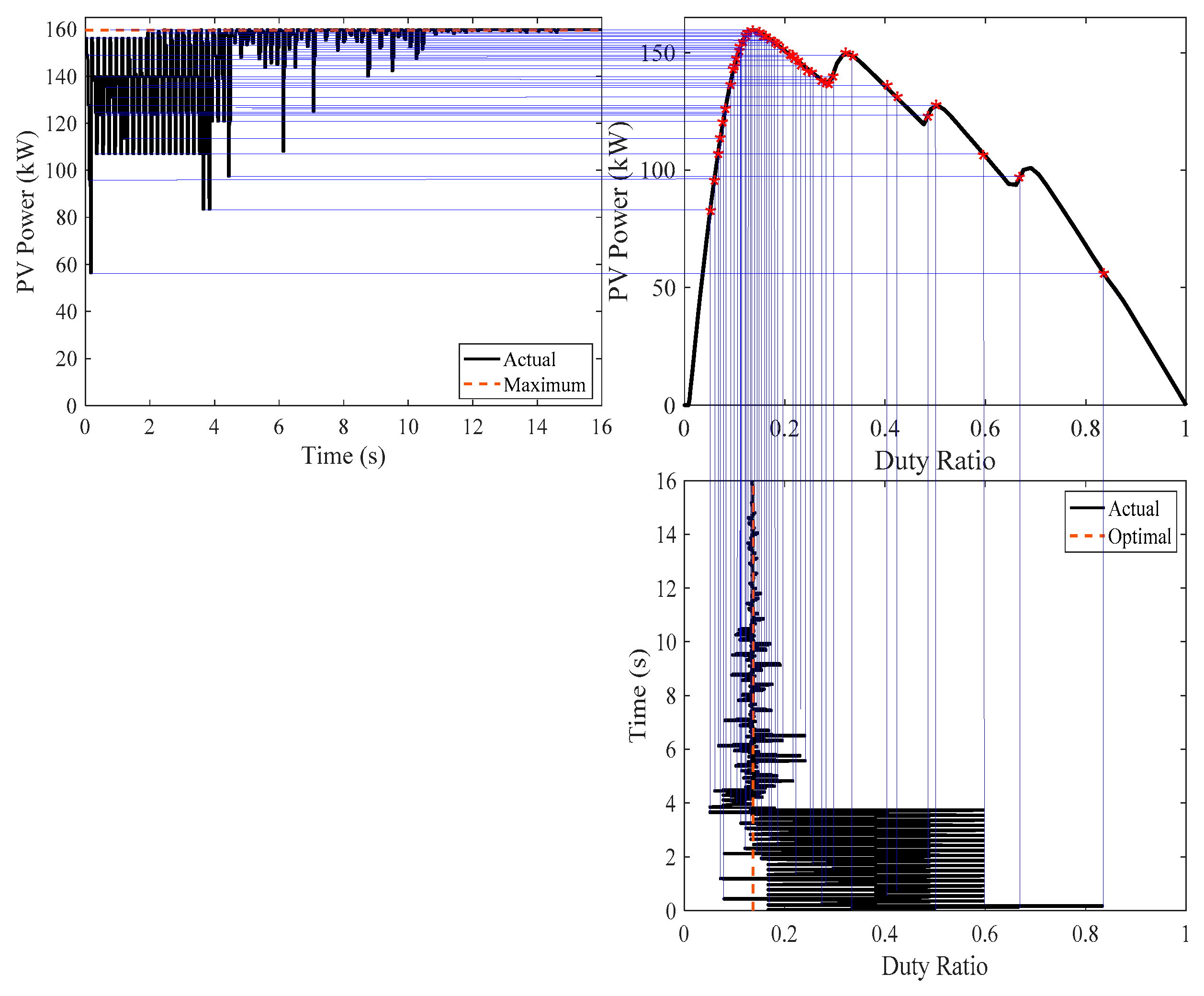
The relation between the PV power from the PV arrays and the duty ratio of the boost converter is shown in Figure 19 for uniform irradiance and partial shading conditions (PSC). For uniform irradiance as shown in SP0 of Figure 19, there is only one peak in the P-V characteristics of PV array. Meanwhile, in the case of PSC, many peaks are generated in the P-V characteristics of the PV array, as shown in SP1-SP3 of Figure 18. Shading patterns based on PSC (SP1-SP3) are having one global peak (GP) and many local peaks (LPs) in each curve. A conventional technique like hill-climbing [47] or perturb and observe [48] are effective in tracking the MPPT of the PV system in uniform irradiance, because there is only one peak. Meanwhile, these techniques may stick at one of the LPs in the case of PSC. For this reason, swarm techniques like the PSO have been used as an MPPT of the PV systems [49,50,51,52,53,54,55,56,57,58,59]. Although these techniques, especially the PSO, showed great improvement; meanwhile, they are suffering from two shortcomings, which are the sluggish convergence and premature convergence possibilities. The main reason for these two shortcomings was the improper selection of the PSO control parameters, which was the main motive to propose a new technique to determine the optimal values of these parameters. The two shortcomings can be measured using the N_SS and PCR. The actual convergence rate of the boost converter is equal to the value of N_SS times the sampling time or switching signal period t_S. The sampling period is chosen in this study to be 0.05 s. The PV system is simulated in Simulink, and the Matlab code of the PSO is simulated in Matlab code. The simulation is carried out for the PV system shown in Figure 18 1000 times to avoid the random nature of PSO. The swarm size is selected to be equal to the maximum number of peaks in the P-V characteristics, which is recommended in the literature [46,50]. For this reason, the swarm size is chosen to be equal to five. Random initialization for the values of duty ratios of boost converter prolongs the convergence rate and increases the value of PCR, and for this reason, the initialization of duty ratios can be obtained from (14). As an example, if SS = 5, then the initial values of duty ratios are [0.166 0.333 0.5 0.667 0.833]. The boundaries for the inner loop variables (duty ratio of boost converter) are set between 0.02 to 0.98. Regarding the variables of the outer PSO loop variables that will be used as input to the inner PSO loop, the boundaries of these PSO control parameters are selected as the same for the benchmark function.

$$d_k=\frac{k}{SS+1}$$

(14)

where, k is the counter representing the particles of the swarm, k = 1, 2, … SS, and SS is the swarm size.

The simulation is performed for the same strategies shown in Table 5 compared to the results obtained from NESTPSO, and the results are shown in

Table 6. The performance evaluation of the PSO with state-of-the-art strategies and the NESTPSO.

	Parameters	ωι	cli	cgi	tc (s)	PCR (%)	% Reduction by NESTPSO
Strategy
S1 [8]		0.72980;	1.49618	1.49618	13.38600	0.00000	383.73810
S2 [9]		0.72900	1.49445	1.49445	13.28518	0.00000	380.09470
S3 [10]		0.71500	1.70000	1.70000	15.01750	0.00000	442.69660
S4 [12]		0.72900	2.05000	2.05000	14.43200	0.00000	421.53800
S5 [11]		0.72900	2.04120	0.94770	12.62018	0.00000	356.06320
S6 [12]		0.72400	1.46800	1.46800	12.78300	0.00000	361.94710
S7 [13]		0.72000	1.10800	1.10800	9.68083	0.00000	249.84190
S8 [14]		0.42000	1.55000	1.55000	5.17117	0.00000	86.87390
S9 [15]		0.50000	1.90000	1.90000	10.15718	0.00000	267.05620
S10 [15]		0.60000	1.80000	1.80000	12.64768	0.00000	357.05700
NESTPSO		−0.00450	−0.0028	1.45720	2.76720	0.00000	0.00000

. The multiobjective function is as shown in (8), where M is chosen to be equal to 1000. It is clear from the results obtained that the PCR is equal to zero for all strategies under study thanks to initialization from Equation (14), and the evaluation of these strategies will be based on the convergence time t_C. It is clear from the results shown in Table 6 that the longest convergence time is 15.0175 s for S3 [10] strategy. Meanwhile, the shortest convergence time is 5.171175 s for S8 [14] strategy. The simulation used to determine the optimal PSO control parameter values using the NESTPSO is started in the beginning using the same logic discussed above. The values of the control parameter obtained from the NESTPSO are used online to see the convergence time for online control where random radiations are chosen for the 5 PV module groups are used. The convergence time with the NESTPSO strategy is 2.7672 s, which is less than half the convergence time of the best state-of-the-art strategy shown in Table 6. This reduction in convergence time shows the superiority of using the NESTPSO in many online optimization applications where the fast response of this strategy allows the PSO to work effectively with the fast-changing weather conditions.

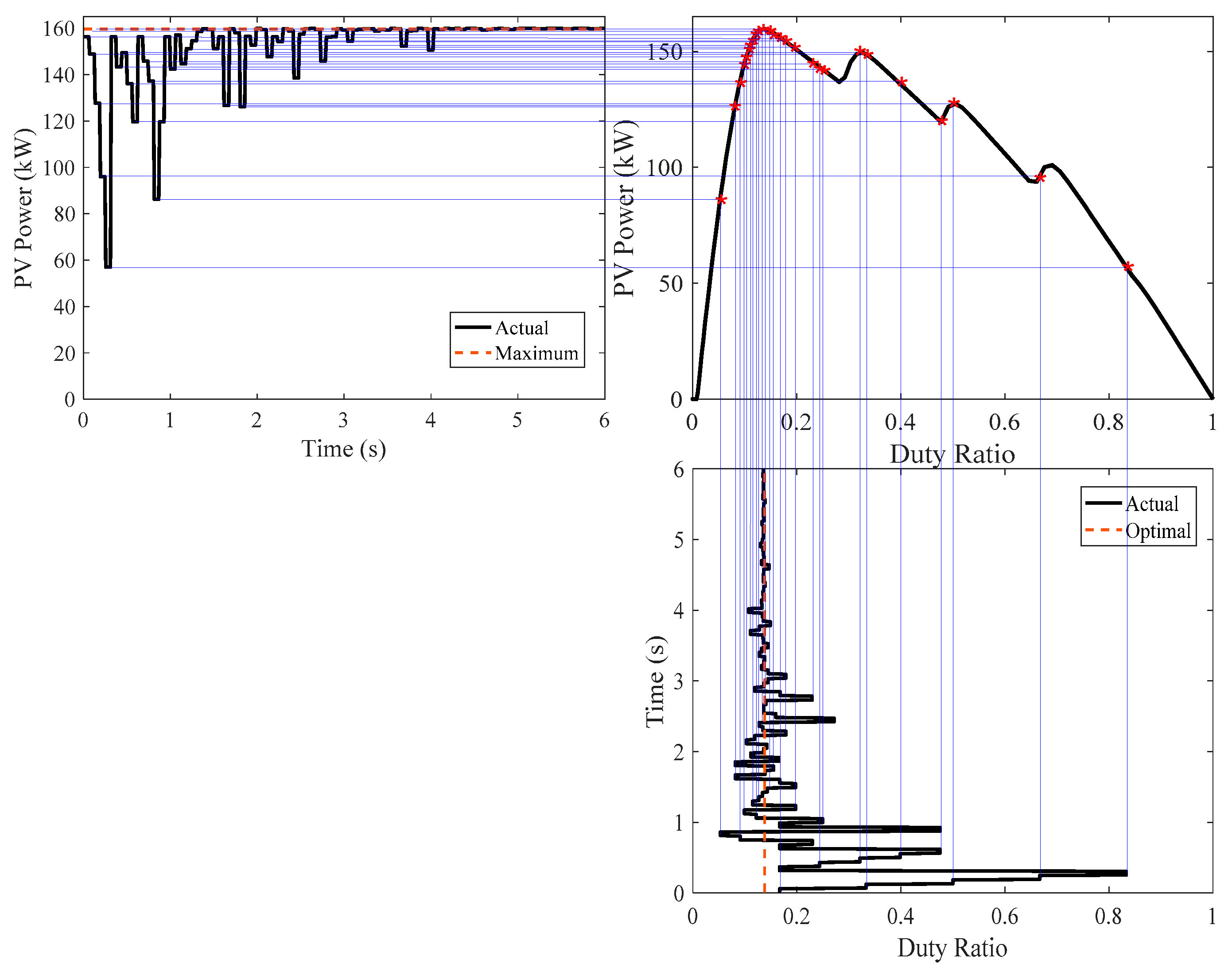
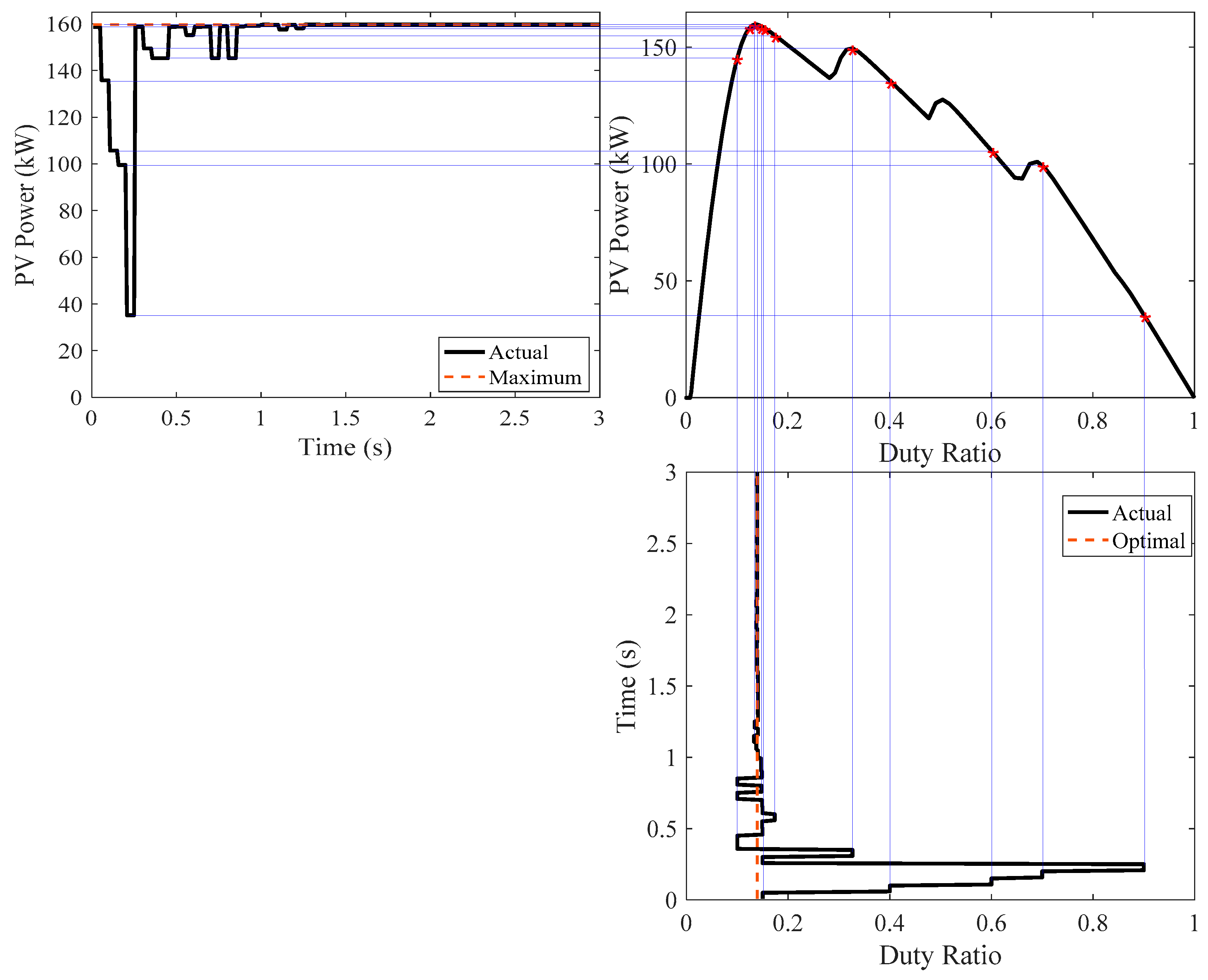
To show the superiority of performance of the NESTPSO in MPPT of the PV system, it will be compared to the longest convergence (S3 [10]) and shortest convergence (S8 [14]) time strategies. Figure 20 shows the performance of the PV system with the longest convergence time (S3 [10]) state-of-the-art strategy. It is clear from this figure that the PSO captured the GP after 15.02 s convergence time. Figure 21 shows the performance of the PV system with the shortest convergence time (S8 [14]) state-of-the-art strategy. It is clear from this figure that the PSO captured the GP after 5.17 s convergence time. Figure 22 shows the performance of the PV system with the control parameters obtained from NESTPSO. It is clear from this figure that the NESTPSO strategy captured the GP with 2.76 s, which is substantially lower than the convergence time from all state-of-the-art strategies, which proved the superiority of the NESTPSO in determining the control parameters of the PSO when it is used as an MPPT of the PV energy systems. This reduction in convergence time will enable the PSO and other swarm optimization techniques to work in online tracking of MPPT with very fast performance.

5. Conclusions and Recommendations

Applying the PSO to search for the optimal conditions in any optimization needs high confidence in getting the global optimal solution and a fast convergence rate, especially in the online applications of the PSO. The high confidence of getting the global optimal solution can be achieved by minimizing the PCR and the convergence time. Therefore, the PCR and convergence time are the key issues to evaluate the performance of the PSO or any other metaheuristic technique. These two factors should be minimized for the high performance of the PSO. These two factors are affected considerably by the control parameters of the PSO. Therefore, these two factors are minimized by varying the control parameters of the PSO that can be achieved by using the new proposed strategy (NESTPSO). It comprises of two nested PSO loops. The NESTPSO has been introduced in this study to determine the optimal PSO control parameters offline, and they will be used in online applications. The NESTPSO is performed with four popular benchmark functions to compare it with the existing PSO strategies. The NESTPSO strategy showed a considerable improvement in the performance of the PSO in terms of reduction in the values of the PCR and convergence time. This improvement in the performance of the PSO will further encourage the researchers, designers, and operators to use the PSO and all the metaheuristic optimization techniques in the optimization of many online problems where the inferior performance of these techniques was a barrier in the online applications in the past. With the superior results obtained from the NESTPSO, the metaheuristic techniques will have big support to surpass any other optimization techniques, especially in online applications. In the future, the NESTPSO can be applied to many applications to achieve the optimal values of control parameters of the PSO to improve their performance. The practical applications in real life or engineering optimization issues such as the MPPT of PV energy system shows the superior of the NESTPSO in terms of the convergence time, where it reduced the convergence time from 442.7% to 86.9% compared to the convergence time of state-of-the-art strategies when they are used in the MPPT of the PV systems.

Major conclusions from this study can be summarized in the following points:

• The control parameters have a great effect on the performance of a PSO technique.
• Desired values of control parameters of PSO for a certain fitness function do not guarantee the same for other fitness functions. This means that every fitness function has different values of optimal PSO control parameters for an optimal PSO performance, and it is not recommended to use fixed values of these parameters in all the applications.
• Tuning the PSO parameters needs high expertise designers, and there is no guarantee that these tuned parameters are the best choice. The NESTPSO provides a guarantee that its results of control parameters display the highest performance.
• The proposed strategy exhibits a rapid convergence to reach the optimal solution compared to the time required by the state-of-the-art strategies.
• The optimal value of inertia weight is approximately constant for all the applications and varies from 0.7536 to 0.8764. Meanwhile, the acceleration parameters have widely different values from one fitness function to another.
• The values of PCR and N_SS reduced considerably for all the benchmark functions with NESTPSO, compared to the state-of-the-art strategies.
• The private PSO parameter c_l is sometimes going to a negative value, which is not shown before in the literature.

Suggested applications of NESTPSO in the future are:

• Determining the control parameters for the dynamic variation control parameters in the PSO strategies.
• Determining the control parameters of other metaheuristic techniques.

References

1. Tillman, F.A. The multiple terminal delivery problems with probabilistic demands. Transp. Sci. 1969, 3, 192. [Google Scholar] [CrossRef]
2. Zhang, Y.; Wang, S.; Ji, G. A comprehensive survey on particle swarm optimization algorithm and its applications. Math. Probl. Eng. 2015, 1, 1–38. [Google Scholar] [CrossRef] [Green Version]
3. Kennedy, J.; Eberhart, R. Particle swarm optimization. In Proceedings of the ICNN′95-International Conference on Neural Networks, Perth, WA, Australia, 27 November–1 December 1995; Volume 4, pp. 1942–1948. [Google Scholar]
4. Shi, Y.; Eberhart, R. A modified particle swarm optimizer. In Proceedings of the IEEE International Conference on Evolutionary Computation Proceedings, IEEE World Congress on Computational Intelligence, Anchorage, AK, USA, 4–9 May 1998; pp. 69–73. [Google Scholar]
5. Li, M.; Zhang, M.; Chen, H.; Lu, S. A Method of Biomedical Information Classification based on Particle Swarm Optimization with Inertia Weight and Mutation. Open Life Sci. 2018, 13, 355–373. [Google Scholar] [CrossRef] [Green Version]
6. Zhan, D.; Lu, H.; Hao, W.; Jin, D. Improving particle swarm optimization: Using neighbor heuristic and Gaussian cloud learning. Intell. Data Anal. 2016, 20, 167–182. [Google Scholar] [CrossRef]
7. Zhang, L.; Tang, Y.; Hua, C.; Guan, X. A new particle swarm optimization algorithm with adaptive inertia weight based on Bayesian techniques. Appl. Soft Comput. 2015, 28, 138–149. [Google Scholar] [CrossRef]
8. Clerc, M.; Kennedy, J. The particle swarm-explosion, stability, and convergence in a multidimensional complex space. IEEE Trans. Evol. Comput. 2002, 6, 58–73. [Google Scholar] [CrossRef] [Green Version]
9. Clerc, M. The swarm and the queen: Towards a deterministic and adaptive particle swarm optimization. In Proceedings of the 1999 Congress on Evolutionary Computation-CEC99, Washington, DC, USA, 6–9 July 1999; Volume 3, pp. 1951–1957. [Google Scholar]
10. Jiang, M.; Luo, Y.P.; Yang, Y. Particle swarm optimization-stochastic trajectory analysis and parameter selection. In Swarm Intelligence, Focus on Ant and Particle Swarm Optimization; IntechOpen: Rijeka, Croatia, 2007; pp. 179–198. [Google Scholar]
11. Carlisle, A.; Dozier, G. An off-The-shelf PSO. In Proceedings of the Workshop on Particle Swarm Optimization; Purdue School of Engineering and Technology: Indianapolis, Indiana, 2001. [Google Scholar]
12. Zhang, W.; Ma, D.; Wei, J.; Liang, H. A parameter selection strategy for particle swarm optimization based on particle positions. Expert Syst. Appl. 2014, 41, 3576–3584. [Google Scholar] [CrossRef]
13. Clerc, M. Stagnation Analysis in Particle Swarm Optimisation or What Happens When Nothing Happens; IntechOpen: Rijeka, Croatia, 2006. [Google Scholar]
14. Liu, Q. Order-2 stability analysis of particle swarm optimization. Evol. Comput. 2015, 23, 187–216. [Google Scholar] [CrossRef] [PubMed]
15. Harrison, K.R.; Engelbrecht, A.P.; Ombuki-Berman, B.M. An adaptive particle swarm optimization algorithm based on optimal parameter regions. In Proceedings of the 2017 IEEE Symposium Series on Computational Intelligence (SSCI), Honolulu, HI, USA, 27 November–1 December 2017; pp. 1–8. [Google Scholar]
16. Harrison, K.R.; Andries, P.; Beatrice, E.; Ombuki-Berman, M. Optimal parameter regions and the time-dependence of control parameter values for the particle swarm optimization algorithm. Swarm Evol. Comput. 2018, 41, 20–35. [Google Scholar] [CrossRef] [Green Version]
17. Bonyadi, M.R.; Michalewicz, Z. Stability analysis of the particle swarm optimization without stagnation assumption. IEEE Trans. Evol. Comput. 2015, 20, 814–819. [Google Scholar] [CrossRef]
18. Alireza, A.L.F.I. PSO with adaptive mutation and inertia weight and its application in parameter estimation of dynamic systems. Acta Autom. Sin. 2011, 37, 541–549. [Google Scholar]
19. Cleghorn, C.W.; Andries, P.E. Particle swarm convergence: An empirical investigation. In Proceedings of the 2014 IEEE Congress on Evolutionary Computation (CEC), Beijing, China, 6–11 July 2014; pp. 2524–2530. [Google Scholar]
20. Eberhart, R.C.; Yuhui, S. Comparing inertia weights and constriction factors in particle swarm optimization. In Proceedings of the 2000 Congress on Evolutionary Computation. CEC00 (Cat. No. 00TH8512), La Jolla, CA, USA, 16–19 July 2000; Volume 1, pp. 84–88. [Google Scholar]
21. Van den Bergh, F.; Engelbrecht, A.P. A study of particle swarm optimization particle trajectories. Inf. Sci. 2006, 176, 937–971. [Google Scholar] [CrossRef]
22. Poli, R.; Bratton, D.; Blackwell, T.; Kennedy, J. Theoretical derivation, analysis and empirical evaluation of a simpler particle swarm optimiser. In Proceedings of the 2007 IEEE Congress on Evolutionary Computation, Singapore, 25–28 September 2007; pp. 1955–1962. [Google Scholar]
23. Poli, R. Mean and variance of the sampling distribution of particle swarm optimizers during stagnation. IEEE Trans. Evol. Comput. 2009, 4, 712–721. [Google Scholar] [CrossRef]
24. Tambouratzis, G. PSO Optimal Parameters and Fitness Functions in an NLP Task. In Proceedings of the 2019 IEEE Congress on Evolutionary Computation (CEC), Wellington, New Zealand, 10–13 June 2019; pp. 611–618. [Google Scholar]
25. Eltamaly, A.M.; Mohamed, A.M. Optimal sizing and designing of hybrid renewable energy systems in smart grid applications. In Advances in Renewable Energies and Power Technologies; Elsevier: Amsterdam, The Netherlands, 2018; pp. 231–313. [Google Scholar]
26. Mohamed, M.A.; Eltamaly, A.M. A PSO-Based Smart Grid Application for Optimum Sizing of Hybrid Renewable Energy Systems. In Modeling and Simulation of Smart Grid Integrated with Hybrid Renewable Energy Systems; Springer: Cham, Switzerland, 2018; pp. 53–60. [Google Scholar]
27. Kennedy, J.; Mendes, R. Population structure and particle swarm performance. In Proceedings of the 2002 Congress on Evolutionary Computation. CEC’02 (Cat. No. 02TH8600), Honolulu, HI, USA, 12–17 May 2002; Volume 2, pp. 1671–1676. [Google Scholar]
28. Mendes, R.; Kennedy, J.; Neves, J. The fully informed particle swarm: Simpler, maybe better. IEEE Trans. Evol. Comput. 2004, 8, 204–210. [Google Scholar] [CrossRef]
29. Farh, H.M.H.; Othman, M.F.; Eltamaly, A.M.; Al-Saud, M.S. Maximum power extraction from a partially shaded PV system using an interleaved boost converter. Energies 2018, 11, 2543. [Google Scholar] [CrossRef] [Green Version]
30. Shi, Y.; Eberhart, R.C. Parameter selection in particle swarm optimization. In International Conference on Evolutionary Programming; Springer: Berlin/Heidelberg, Germany, 1998; pp. 591–600. [Google Scholar]
31. Pedersen, M.E. Good Parameters for Particle Swarm Optimization; Tech. Rep. HL1001; Hvass Lab.: Copenhagen, Denmark, 2010; pp. 1551–3203. [Google Scholar]
32. Bansal, J.C.; Singh, P.K.; Saraswat, M.; Verma, A.; Jadon, S.S.; Abraham, A.A. Inertia weight strategies in particle swarm optimization. In Proceedings of the 2011 Third World Congress on Nature and Biologically Inspired Computing, Salamanca, Spain, 19–21 October 2011; pp. 633–640. [Google Scholar]
33. Rathore, A.; Sharma, H. Review on inertia weight strategies for particle swarm optimization. In Proceedings of Sixth International Conference on Soft Computing for Problem Solving; Springer: Singapore, 2017; pp. 76–86. [Google Scholar]
34. Shi, Y.; Eberhart, R.C. Empirical study of particle swarm optimization. In Proceedings of the Proceedings of the 1999 Congress on Evolutionary Computation-CEC99 (Cat. No. 99TH8406), Washington, DC, USA, 6–9 July 1999; Volume 3, pp. 1945–1950. [Google Scholar]
35. Al-Hassan, W.; Fayek, M.B.; Shaheen, S.I. Psosa: An optimized particle swarm technique for solving the urban planning problem. In Proceedings of the 2006 International Conference on Computer Engineering and Systems, Cairo, Egypt, 5–7 November 2006; pp. 401–405. [Google Scholar]
36. Chatterjee, A.; Siarry, P. Nonlinear inertia weight variation for dynamic adaptation in particle swarm optimization. Comput. Oper. Res. 2006, 33, 859–871. [Google Scholar] [CrossRef]
37. Fouad, K.M.; Elsheshtawy, T.; Dawood, M.F. Parallelized linear time variant acceleration coefficients of PSO algorithm for global optimization. In Proceedings of the 2017 12th International Conference on Computer Engineering and Systems (ICCES), Triumph Hotel Cairo, Egypt, 19–20 December 2017; pp. 556–563. [Google Scholar]
38. Geetha, S.; Poonthalir, G.; Vanathi, P.T. Nested particle swarm optimisation for multi-depot vehicle routing problem. Int. J. Oper. Res. 2013, 16, 329–348. [Google Scholar] [CrossRef]
39. Farsadi, M.; Hosseinnejad, H.; Dizaji, T.S. Solving unit commitment and economic dispatch simultaneously considering generator constraints by using nested PSO. In Proceedings of the 2015 9th International Conference on Electrical and Electronics Engineering (ELECO), Bursa, Turkey, 26–28 November 2015; pp. 493–499. [Google Scholar]
40. Jena, R.K. Multi objective task scheduling in cloud environment using nested PSO framework. Procedia Comput. Sci. 2015, 57, 1219–1227. [Google Scholar] [CrossRef] [Green Version]
41. Matsushita, H.; Tomimura, Y.; Kurokawa, H.; Kousaka, T. Period doubling bifurcation point detection strategy with nested layer particle swarm optimization. Int. J. Bifurc. Chaos 2017, 27, 1750101. [Google Scholar] [CrossRef]
42. Eberhart, R.C.; Groves, D.J.; Woodward, J.K. Deep swarm: Nested particle swarm optimization. In Proceedings of the 2017 IEEE Symposium Series on Computational Intelligence (SSCI), Honolulu, HI, USA, 27 November–1 December 2017; pp. 1–6. [Google Scholar]
43. Matsushita, H.; Kinoshita, W.; Kurokawa, H.; Kousaka, T. Nested-layer particle swarm optimization method for bifurcation point detection in non-autonomous systems. Nonlinear Theory Appl. 2019, 10, 289–302. [Google Scholar] [CrossRef] [Green Version]
44. Eltamaly, A.M.; Al-Saud, M.S. Nested multi-objective PSO for optimal allocation and sizing of renewable energy distributed generation. J. Renew. Sustain. Energy 2018, 10, 035302. [Google Scholar] [CrossRef]
45. Hashim, N.; Salam, Z. Critical evaluation of soft computing methods for maximum power point tracking algorithms of photovoltaic systems. Int. J. Power Electron. Drive Syst. 2019, 10, 548. [Google Scholar] [CrossRef]
46. Farh, H.; Eltamaly, A.M.; Al-Saud, M.S. Interleaved boost converter for global maximum power extraction from the photovoltaic system under partial shading. IET Renew. Power Gener. 2019, 13, 1232–1238. [Google Scholar] [CrossRef]
47. Eltamaly, A.M.; El-Tamaly, H.H.; Enjeti, P. An improved maximum power point tracker for photovoltaic energy systems. In Proceedings of the 2nd Minia International Conference for Advanced Trends in Engineering, Minia, Egypt, 7–9 April 2002. [Google Scholar]
48. Ahmed, J.; Salam, Z. An enhanced adaptive P&O MPPT for fast and efficient tracking under varying environmental conditions. IEEE Trans. Sustain. Energy 2018, 9, 1487–1496. [Google Scholar]
49. Eltamaly, A.M.; Al-Saud, M.S.; Abokhalil, A.G.; Farh, H. Simulation and experimental validation of fast adaptive particle swarm optimization strategy for photovoltaic global peak tracker under dynamic partial shading. Renew. Sustain. Energy Rev. 2020, 124, 109719. [Google Scholar] [CrossRef]
50. Eltamaly, A.M.; Al-Saud, M.S.; Abo-Khalil, A.G. Performance Improvement of PV Systems’ Maximum Power Point Tracker Based on a Scanning PSO Particle Strategy. Sustainability 2020, 12, 1185. [Google Scholar] [CrossRef] [Green Version]
51. Eltamaly, A.M.; Farh, H.; Abokhalil, A.G. A novel PSO strategy for improving dynamic change partial shading photovoltaic maximum power point tracker. Energy Sources Part A Recovery Util. Environ. Eff. 2020, 1–15. [Google Scholar] [CrossRef]
52. Motahhir, S.; Chouder, A.; El Hammoumi, A.; Benyoucef, A.S.; El Ghzizal, A.; Kichou, S.; Kara, K.; Sanjeevikumar, P.; Silvestre, S. Optimal energy harvesting from a multistrings PV generator based on artificial bee colony algorithm. IEEE Syst. J. 2020. [Google Scholar] [CrossRef]
53. Eltamaly, A.M.; Al-Saud, M.S.; Abokhalil, A.G.; Farh, H.M. Photovoltaic maximum power point tracking under dynamic partial shading changes by novel adaptive particle swarm optimization strategy. Trans. Inst. Meas. Control 2020, 42, 104–115. [Google Scholar] [CrossRef]
54. Eltamaly, A.M. Performance of smart maximum power point tracker under partial shading conditions of photovoltaic systems. J. Renew. Sustain. Energy 2015, 7, 043141. [Google Scholar] [CrossRef]
55. Motahhir, S.; Hammoumi, A.E.; Ghzizal, A.E.; Derouich, A. Open hardware/software test bench for solar tracker with virtual instrumentation. Sustain. Energy Technol. Assess. 2019, 31, 9–16. [Google Scholar] [CrossRef]
56. Eltamaly, A.M. Performance of MPPT techniques of photovoltaic systems under normal and partial shading conditions. In Advances in Renewable Energies and Power Technologies; Elsevier: Amsterdam, The Netherlands, 2018; pp. 115–161. [Google Scholar]
57. Eltamaly, A.M.; Farh, H.M.; Othman, M.F. A novel evaluation index for the photovoltaic maximum power point tracker techniques. Solar Energy 2018, 174, 940–956. [Google Scholar] [CrossRef]
58. Farh, H.M.; Eltamaly, A.M.; Othman, M.F. Hybrid PSO-FLC for dynamic global peak extraction of the partially shaded photovoltaic system. PLoS ONE 2018, 13, e0206171. [Google Scholar] [CrossRef] [PubMed]
59. Eltamaly, A.M.; Farh, H.; Al Saud, M. Impact of PSO reinitialization on the accuracy of dynamic global maximum power detection of variant partially shaded PV systems. Sustainability 2019, 11, 2091. [Google Scholar] [CrossRef] [Green Version]
Figure 1. NESTPSO outer PSO loop flowchart.
Sustainability 13 01008 g001
Figure 2. NESTPSO inner PSO loop flowchart.
Sustainability 13 01008 g002
Figure 3. Pseudo-code for the outer PSO loop in NESTPSO.
Sustainability 13 01008 g003
Figure 4. Pseudo-code for the inner PSO loop in NESTPSO.
Sustainability 13 01008 g004
Figure 5. The 3-D pslot of the benchmark function with D = 2. (a) sphere function. (b) Rastrigrin function. (c) De Jong function. (d) Alpine function.
Sustainability 13 01008 g005aSustainability 13 01008 g005b
Figure 6. Variation of M with the performance parameters of the inner PSO loop for the Sphere function.
Sustainability 13 01008 g006
Figure 7. Relation of Ni, SSi, and Nss with PCR for the Sphere function.
Sustainability 13 01008 g007
Figure 8. Variation of M with the performance parameters of the inner PSO loop for the Rastrigrin function.
Sustainability 13 01008 g008
Figure 9. Relation of Ni, SSi, and NSS with PCR for the Rastrigrin function.
Sustainability 13 01008 g009
Figure 10. Variation of M with the performance parameters of the inner PSO loop for the De Jong function.
Sustainability 13 01008 g010
Figure 11. Relation of Ni, SSi, and Nss with PCR for the De Jong function.
Sustainability 13 01008 g011
Figure 12. Relation of Ni, SSi, and Nss with PCR for the Alpine function.
Sustainability 13 01008 g012
Figure 13. Variation of M with the performance parameters of the inner PSO loop for the Alpine function.
Sustainability 13 01008 g013
Figure 14. Fitness function value against NSS for the Sphere function.
Sustainability 13 01008 g014
Figure 15. Fitness function value against NSS for the Rastrigrin function.
Sustainability 13 01008 g015
Figure 16. Fitness function value against NSS for the De Jong function.
Sustainability 13 01008 g016
Figure 17. Fitness function value against NSS for Alpine function.
Sustainability 13 01008 g017
Figure 18. The PV energy system with a PSO-based MPPT.
Sustainability 13 01008 g018
Figure 19. Power vs duty ratio of the boost converter with five modules in series having different irradiances.
Sustainability 13 01008 g019
Figure 20. Performance of PSO MPPT of PV system with the parameter of S3 [10] as shown in Table 6.
Sustainability 13 01008 g020
Figure 21. Performance of PSO MPPT of the PV system with the parameter of S8 [14] as shown in Table 6.
Sustainability 13 01008 g021
Figure 22. Performance of PV energy system using NESTPSO as an MPPT strategy.
Sustainability 13 01008 g022