Article

A Quantitative Modeling and Prediction Method for Sustained Rainfall-PM2.5 Removal Modes on a Micro-Temporal Scale

1
Faculty of Geomatics, Lanzhou Jiaotong University, Lanzhou 730070, China
2
National-Local Joint Engineering Research Center of Technologies and Applications for National Geographic State Monitoring, Lanzhou 730070, China
3
Gansu Provincial Engineering Laboratory for National Geographic State Monitoring, Lanzhou 730070, China
4
Faculty of Geosciences and Environmental Engineering, Southwest Jiaotong University, Chengdu 611756, China
5
Key Lab for Environmental Computation and Sustainability of Liaoning Province, Institute of Applied Ecology, Chinese Academy of Sciences, Shenyang 110016, China
*
Author to whom correspondence should be addressed.
Sustainability 2021, 13(19), 11022; https://doi.org/10.3390/su131911022
Submission received: 27 August 2021 / Revised: 30 September 2021 / Accepted: 1 October 2021 / Published: 5 October 2021
(This article belongs to the Topic Climate Change and Environmental Sustainability)

Abstract

:
PM2.5 is unanimously considered to be an important indicator of air quality. Sustained rainfall is a kind of typical but complex rainfall process in southern China with an uncertain duration and intervals. During sustained rainfall, the variation of PM2.5 concentrations in hour-level time series is diverse and complex. However, existing analytical methods mainly examine overall removals at the annual/monthly time scale, missing a quantitative analysis mode that applies micro-scale time data to describe the removal phenomenon. In order to further achieve air quality prediction and prevention in the short term, it is necessary to analyze its micro-temporal removal effect for atmospheric environment quality forecasting. This paper proposed a quantitative modeling and prediction method for sustained rainfall-PM2.5 removal modes on a micro-temporal scale. Firstly, a set of quantitative modes for sustained rainfall-PM2.5 removal mode in a micro-temporal scale were constructed. Then, a mode-constrained prediction of the sustained rainfall-PM2.5 removal effect using the factorization machines (FM) was proposed to predict the future sustained rainfall removal effect. Moreover, the historical observation data of Nanjing city at an hourly scale from 2016 to January 2020 were used for mode modeling. Meanwhile, the whole 2020 year observation data were used for the sustained rainfall-PM2.5 removal phenomenon prediction. The experiment shows the reasonableness and effectiveness of the proposed method.

1. Introduction

Air pollution is currently a major environmental challenge for both developed and developing countries worldwide, with increasing industrialization, growing urbanization and energy consumption posing a serious threat to public health [1,2]. According to a report from the World Health Organization, PM2.5 is unanimously considered to be an important indicator of air quality [3,4]. The rainfall processes are typically regarded as strong drivers to remove PM2.5 so as to improve the air quality.
However, in the existing available research on an observation data analysis, there are obvious inconsistency between rainfall and the PM2.5 removal effect, especially for sustained rainfall, a kind of typical but complex rainfall process in southern China with an uncertain duration and intervals. For example, Kao et al. [5] found that in a rainforest environment, summers with high precipitation are negatively correlated with PM2.5 levels; Preethi et al. [6] proposed that the effect of simulated Indian monsoon rainfall removal depends to a large extent on climatic wind speeds; Neal et al. [7] pointed out that there has been no systematic improvement in air quality in mid Wales for 17 years in the face of increased rainfall. In addition to the complexity of the sustained rainfall itself, the variations in regional environmental conditions are possibly another important reason. Therefore, studying the relationship between sustained rainfall and the PM2.5 removal effect becomes a multi-factor related scientific issue.
When expressing the effect of rainfall on the removal of PM2.5 concentrations in the air, the observed time series is usually the most intuitive expression [8,9]. The observed value will be considered as a sign of the presence of the rainfall process [10]. However, sustained rainfall, which is characterized by two or more sustained rainfall events within a given period of time, is intermittent, slow to change and uncertain in its length of formation, and its complexity needs to be fully considered [11,12]. During sustained rainfall, the variation of PM2.5 concentrations in hour-level time series is diverse and complex. However, existing analytical methods mainly examine overall removals at the annual/monthly time scale and mainly use the correlation analysis (CA) between rainfall amount and PM2.5 concentration based on macroscopic monitoring data, which refers to the rainfall time series and PM2.5 time series sampled on an annual or monthly temporal scale [13,14]. For example, using the data of a macro-temporal scale, Shaibu et al. [15] confirmed that monthly PM2.5 concentrations in the Niger Delta region of Nigeria show a significant positive correlation with monthly rainfall. Similarly, through a study of annual datasets from five air quality monitoring stations in Bahrain from 2006 to 2012, Jassim et al. [16] indicated little correlation between rainfall and PM2.5, leading to a year-on-year increase in PM2.5 concentrations. They are all missing a quantitative analysis mode that applies micro-scale time data to describe the removal phenomenon. In order to further achieve air quality prediction and prevention in the short term, it is necessary to analyze its micro-temporal removal effect for atmospheric environment quality forecasting.
In addition, due to the sustained rainfall and the atmospheric pollution particulate matter itself being complex, the large-scale temporal analysis lacks guidance for specific sustained rainfall-PM2.5 removal processes [17]. On this basis, a part of the study proposes to extract the historical single rainfall process using hourly observation data and adopt a predetermined calculation model to quantify the removal effect of the rainfall process: Chhavi et al. [18] analyzed the wet removal effect by calculating the PM2.5 concentration difference before and after rainfall, including the positive and negative removal; Kapwata et al. [19], based on the intensity of rainfall, delineate the rainfall classes, counting the percentage of positive removal to summarize the removal effect according to the influence factors, such as rainfall duration and rainfall volume, which have certain guiding significance. The above methods do not take into account the changes in the effects produced by complex sustained rainfall processes at different stages, including effects such as hygroscopic growth and the secondary transformation of gaseous pollutants which cause PM2.5 concentrations to rise or rebound [20,21,22]; at the same time, they lack universal law exploration, having difficulties in serving the scientific prediction and early warning of air quality systems and active prevention [23,24].
In this paper, we propose a quantitative modeling and prediction method for sustained rainfall-PM2.5 removal modes on a micro-temporal scale. The detailed contributions are as follows:
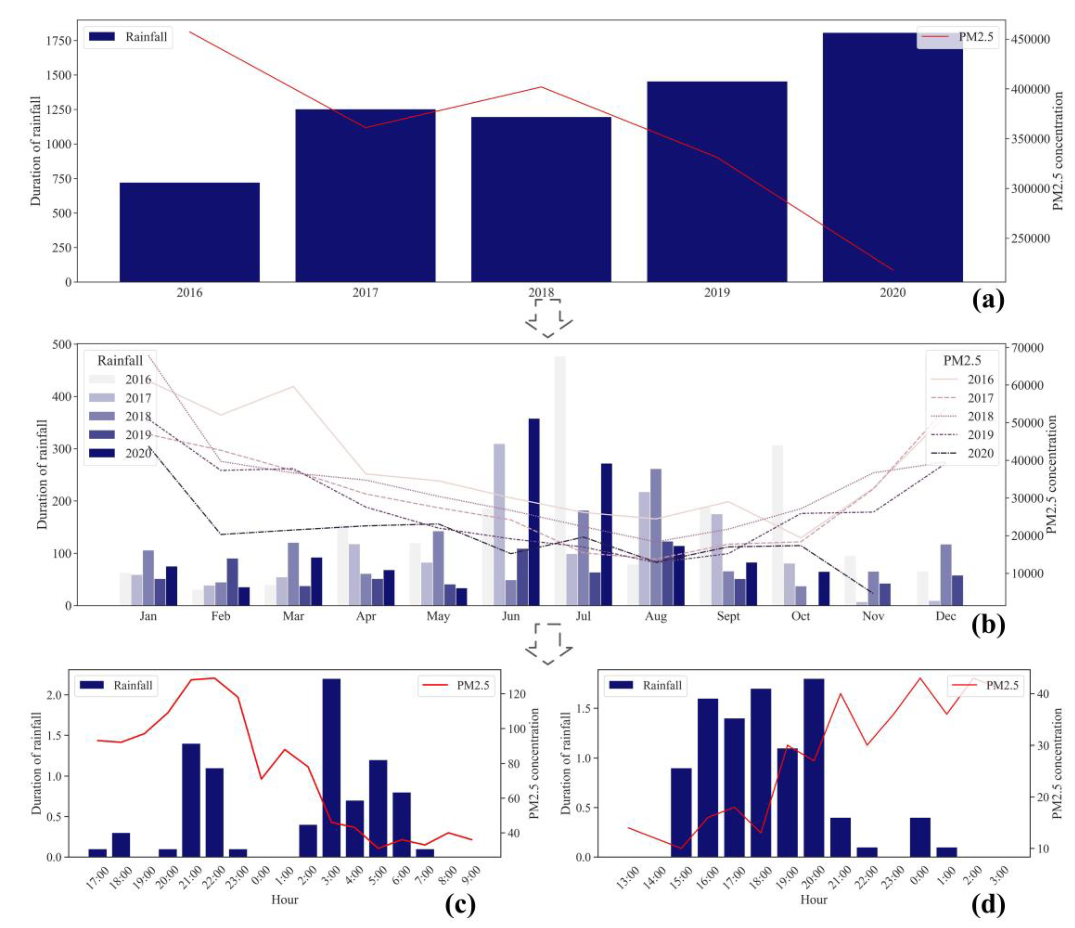
  • A novel micro-scale analytical framework for quantitatively elucidating the mechanism of PM2.5 removal by sustained rainfall was proposed. Compared with the yearly, monthly and daily time scales, the hourly scale is a more suitable form of information for decision making; therefore, the framework would more clearly express the complex characteristics of sustained rainfall than the analysis methods of large-scale data. The innovative hourly scale data analysis in this paper is more useful for practical applications in predicting and assessing air quality.
  • A set of quantitative PM2.5 removal modes based on a micro-analysis are proposed. The modes would highlight the specific and high-level patterns of the removal effect of sustained rainfall at the micro-scale than the traditional micro-scale data analysis methods. During sustained rainfall, the variation of PM2.5 concentrations in an hourly time series is diverse and complex. The analysis of hourly scales reveals new characteristic modes that are different from the traditional large scale. These "declining, rebounding, or rising" modes not only allow the analysis of historical data from different regions, but also allow the prediction of PM2.5 removal at hourly intervals using future hourly rainfall, which can help the relevant systems and departments to make timely decisions on air pollution control.
This paper is organized as follows. The study area and data on analytical framework are viewed in Section 2. Section 3 introduces the quantitative definition of the sustained rainfall-PM2.5 removal mode on a micro-temporal scale, then presents the rainfall-PM2.5 removal phenomenon predicting algorithm based on the quantitative model and Section 4 discusses the experimental results. Finally, the discussions are presented in Section 5.

2. Study Area and Data

2.1. Study Area

The experimental area of this paper is located in Nanjing, which is in the middle of the lower reaches of the Yangtze River and has a subtropical monsoon climate with cold and dry winters, high temperatures and rainy summers and a relatively large rainfall variability, making it one of the regions in China with more droughts and floods [25,26]. Some studies have shown that (i) due to the influence of strong convective weather and global warming, there is a significant increase in the amount and duration of rainfall in Nanjing, which has a different degree of the purifying effect on air pollutants [27]; (ii) at the same time, according to the results of a pollutant source analysis in Nanjing, PM2.5 water-soluble ion concentrations have diurnal and seasonal differences, making the average mass concentration of water-soluble ions higher during the day than at night, and the flushing effect of spring and summer rainfall is generally lower than that of autumn and winter [28,29]; (iii) according to the statistics, the annual average humidity in Nanjing is nearly 80%, and some rainfall in this environment may lead to hygroscopic growth of particulate matter, resulting in higher pollutant concentrations [30].

2.2. Dataset

The experimental data in this paper were obtained from hourly PM2.5 concentrations and meteorological observations released by the China General Environmental Monitoring Station and the National Meteorological Information Centre for the period from January 2016 to December 2020. Based on the geographical location of the monitoring stations in Nanjing and the completeness of the data, the PM2.5 data observed at the CCM (Caochangmen) site (32.0572 °N, 118.7486 °E) and the rainfall data observed at the PK (Pukou) site (32.177 °N, 118.706 °E) were used for the experiment.
Figure 1 demonstrates the phenomenon of PM2.5 concentration removal by rainfall observed on a macro-temporal scale (yearly and monthly) to a micro-temporal scale (hourly): from the annual scale, the average annual PM2.5 concentration in Nanjing decreases year by year from 2016 to 2020, while the pollutant concentration is relatively lower in years with a higher average annual rainfall; from the monthly scale, the monthly rainfall shows an overall stable trend of first increasing and then decreasing, and the average monthly PM2.5 concentration in the period of concentrated rainfall are significantly lower than those during periods of low rainfall, indicating that rainfall has a significant effect on the removal of air pollutants; on an hourly scale, the hour-by-hour PM2.5 concentration changes during a single rainfall process, thus rainfall has an obvious effect on pollutant removal while there are situations that cause concentrations to increase, and it is not possible to obtain the mode of the effect of regional rainfall on PM2.5 from a particular rainfall process. In summary, the mechanism of PM2.5 removal by sustained rainfall in Nanjing is complex, and it is difficult to satisfy the study of the mechanism of PM2.5 removal by rainfall with the macro time statistics and the time series of a single rainfall process, so the micro time-series effect model proposed in this paper is applied for a deeper analysis.

3. Methods

3.1. A Quantitative Modeling for Sustained Rainfall-PM2.5 Removal Mode in Micro-Temporal Scale

3.1.1. Overview

In order to accurately describe the study object and the study boundary from the observation dataset, this section first defines a microscopic time-series fragment model of the sustained rainfall process, on the basis of which the time-series process of the removal effect is structured, further modeling the concomitant factors affecting the role of rainfall in PM2.5 removal, and finally establishes an evaluation mode to quantitatively describe the removal effect.

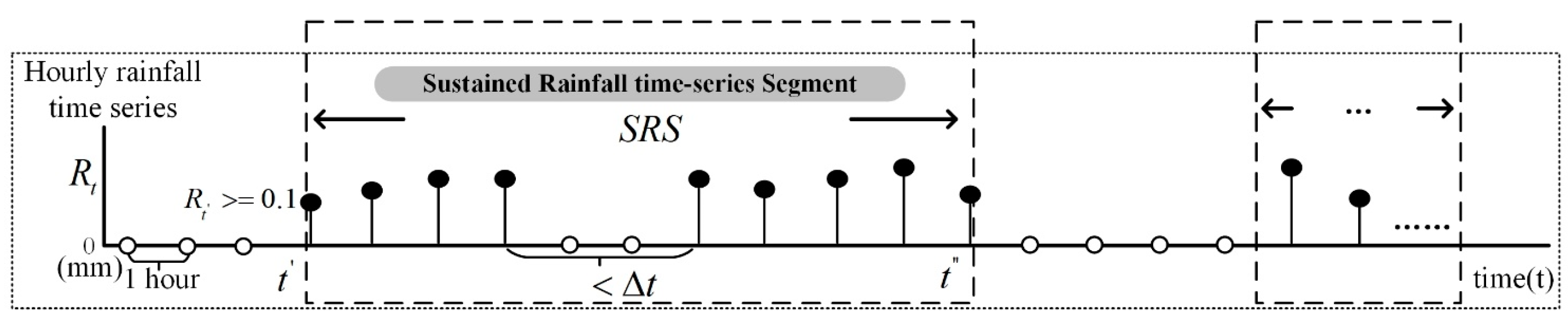
3.1.2. Micro-Temporal Modeling of Sustained Rainfall Process

The model needs to accurately identify a complete sustained rainfall process in micro-scale observations due to the large variation in time duration and the existence of uncertain intervals. The sustained rainfall process is characterized by intermittent multi-fragmentation on hourly observation data series.
Time-series segments (TS) are mathematical frameworks for describing and modeling event sequences in the time domain, and are commonly used to construct interpretable time-series analysis models, such as trend prediction and anomaly detection [31,32]. In this paper, the sustained rainfall time-series segment (SRS) is defined at the micro-temporal scale rainfall: { R t : t = h o u r } . SRS visualizes the variation of rainfall in the time dimension of a sustained rainfall process, as shown in Figure 2, and is defined as follows:
S R S = { [ R t , , R t ] | t , t , t }
The quantitative measurement steps are:
  • Step 1: Using the hourly rainfall values as a benchmark, the moment of the first occurrence of 0.1 mm and above rainfall is taken as the starting point t of the time-series fragment.
  • Step 2: Since rainfall and its resulting effects will remain in space for a certain period of time, a threshold value t is set to indicate the intermittent duration of the sustained rainfall process, i.e., the sequence before and after when rainfall is zero does not exceed t is regarded as the same time-series fragment.
  • Step 3: Satisfy the above conditions and the last occurrence of rainfall greater than zero is the end point t , and obtain a complete S R S .
The micro-temporal model of the sustained rainfall process provides a quantitative basis for determining the baseline interval for the clearance effect analysis.

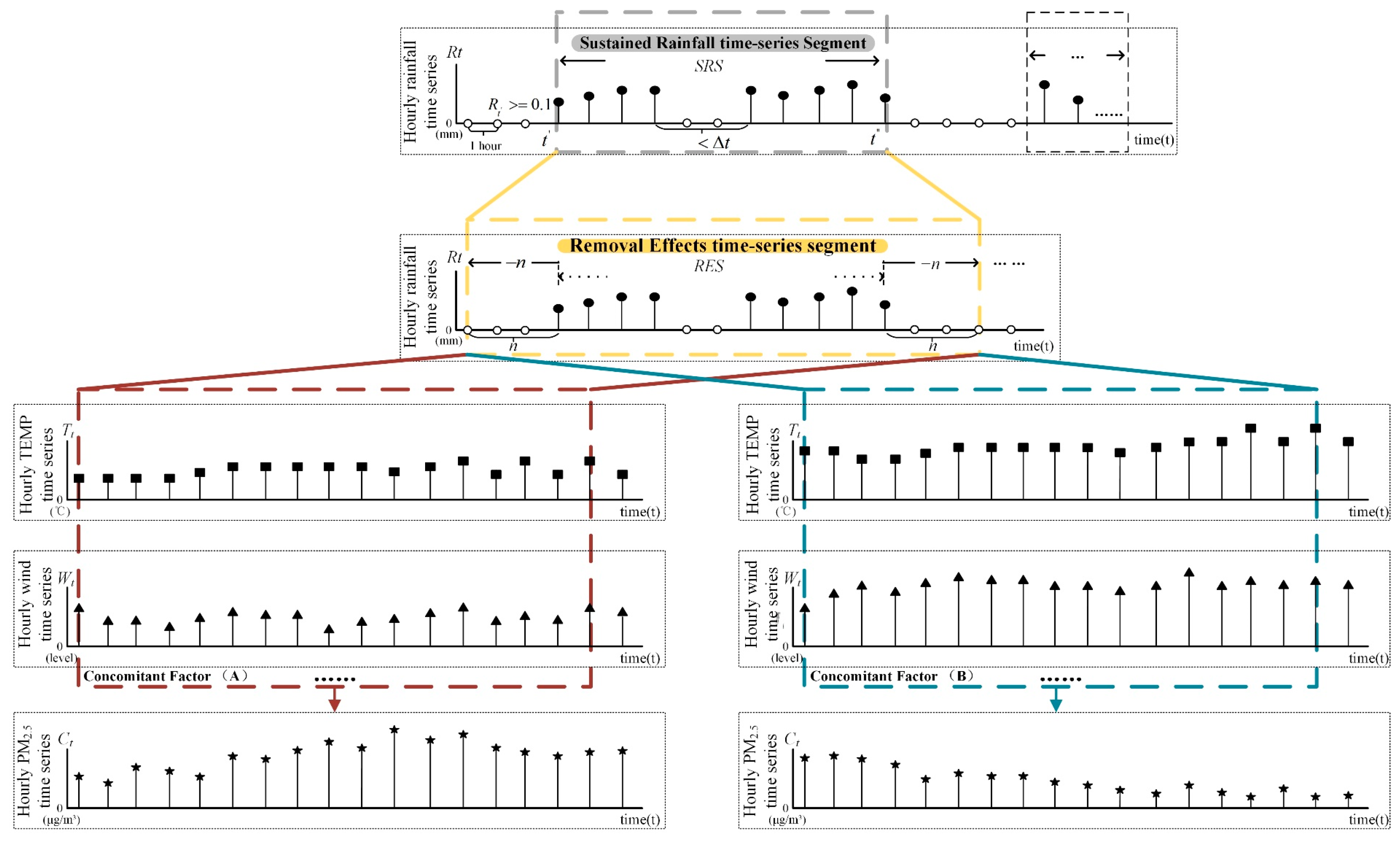
3.1.3. Sustained Rainfall Removal Concomitant Factor Modeling

Sustained rainfall processes are often concomitant by changes in the accompanying meteorological factors such as temperature, humidity, wind speed and direction, which will affect the removal effect to varying degrees [33]. Therefore, in this paper, we consider the effect and intensity of the existing influence factors [34,35,36,37], and balance the availability of their own observational data and the predictability of future trends to establish a set of accompanying influence factors F, including the (i) direct factor (FD) to describe rainfall characteristics, and the (ii) indirect factor (FI) to describe environmental characteristics. The factors and impact effects are shown in Table 1.
On this basis, the removal effects time-series segment (RES) is defined in conjunction with the PM2.5 time series. The RES refers to the process and subsequent effects of rainfall on PM2.5 at the scale of the mechanism of removal, while avoiding the chance of PM2.5 concentration values before rainfall anomalies by expanding the series values for t and t forward and backward for n hours, respectively (Figure 3):
The concomitant factor model { F , R E S } for sustained rainfall removal identifies the information dimensions and effect intervals for the quantitative modeling.

3.1.4. Quantitative Evaluation Modeling of Removal Effects

The effect evaluation refers to the evaluation of the change in the effect produced by a geographical process considering the influence of relevant factors, and usually uses quantitative indicators to measure and analyze its dynamic change characteristics in spatial and temporal modes [38,39]. The quantitative evaluation model of removal effects is proposed based on the above-mentioned models ( S R S , R E S ) :
M = { M i ( T , P , D , U , R , L ) | R P , R F , R S , ( T S R , T S E ) }
(1) Quantitative Measurement of Removal Effect Indicators
Based on the model ( S R S , R E S ) , the following measurable evaluation indicators ( R P , R F , R S ) that quantitatively characterize the temporal variability in the removal processes are defined below:
(i)
Rate of process RP, the ratio of the difference between the very small value of PM2.5 concentration change when it exists and the pre-start PM2.5 concentration.
(ii)
Rate of final RF, the ratio of the difference between the initial PM2.5 concentration before the start and the concentration after the end, the magnitude of which allows a quantitative evaluation of the intensity of removal.
(iii)
Rate of rebound RR, the ratio of the difference between the minimum value and the ending concentration for the entire rainfall process.
(2) Modeling of Removal Mode based on Effect Indicators
The ( S R S , R E S ) and ( R P , R F , R R ) were used to modeling the removal process of sustained rainfall and the indicators were combined with zero boundaries, corresponding to the rising and falling changes in PM2.5 concentrations in Figure 4, and combined with the ensemble theory to classify the effect patterns in Table 2.
The removal mode, classified according to the above rules, covers all of the combinations of indicators and corresponds to realistic removal phenomena, providing a category a priori information for predicting future sustained rainfall.

3.2. The Mode Predicting of Sustained Rainfall-PM2.5 Removal Effect Using the Quantitative Model
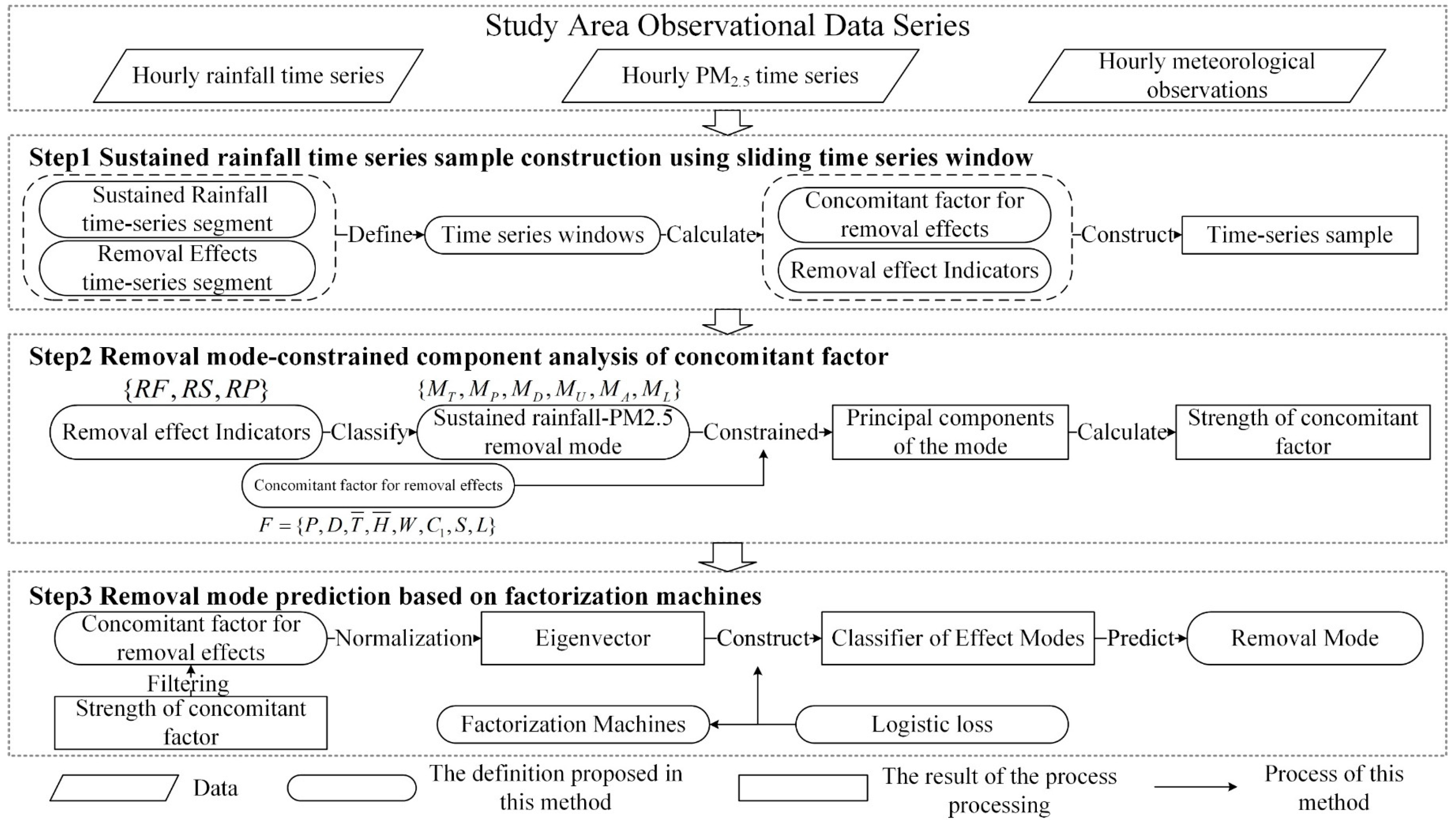
3.2.1. Overview

In this section, based on the quantitative model of sustained rainfall-PM2.5 removal mode, the future rainfall is further fitted using a multiple regression to fit the removal modes, the core steps are as follows (Figure 5): Step 1, using the time-series window according to the constitute time-series sample of removal modes with high-dimensional characteristics; Step 2, extracting the principal components and component features of the pattern classification features through the principal component analysis method for the concomitant factor intensity; Step 3, establishing factorization classification regression machines for removal modes according to the factor intensity, which can predict the removal phenomenon based on the future meteorological and current air quality information.

3.2.2. Sustained Rainfall Time-Series Sample Construction Using Sliding Time-Series Window

Firstly, according to the definitions of the S R S and R E S proposed in Section 3.1, a small-scale sliding window is applied to process the hourly rainfall time series R t , hourly PM2.5 time series C t and hourly meteorological observations, setting up to capture all of the sustained rainfall processes in the historical data [40].
Secondly, the statistics of the corresponding direct and indirect factors are calculated within the extracted time-series range ( S R S , R E S ) according to the concomitant factor model F proposed in this paper, as Table 3.
The quantitative evaluation indicators ( R P , R F , R R ) of the extracted sustained rainfall processes were calculated based on the PM2.5 concentration series C t according to the evaluation model of removal effects described in this paper.
{ R P = ( C 1 C m i n ) C 1 R R = ( C 2 C m i n ) C 2 R F = ( C 1 C 2 ) C 1
C 2 = t = t t + n C t n
C m i n = m i n ( C t , , C t )
where C 1 is the initial PM2.5 concentration during the sustained rainfall process, C 2 is the PM2.5 concentration at the end of the sustained rainfall process and C m i n is the minimum value for the whole sustained rainfall process.
Finally, sustained rainfall time-series samples V were constructed in the form of multi-dimensional feature vectors, as follows:
V = ( P , D , T , ¯ H ¯ , W , C 1 , S , K , [ R F , R S , R P ] )
It provides a computable basis for the accurate extraction of analytical reference intervals from hourly observations.

3.2.3. Removal Mode-Constrained Component Analysis of Concomitant Factor

According to the removal mode division rules in Table 2, the V were classified to obtain six types of labeled samples corresponding to M i , as shown in the following equation. Due to the different degrees of influence of the removal factors on effect indicators in different effect modes, such as the change of effective removal rate magnitude with increasing rainfall duration in complete removal mode, a multi-factor analysis is needed to explore its change pattern.
V = ( P , D , T , ¯ H ¯ , W , C 1 , S , K | M i )
The principal component analysis is a statistical method that reduces the information of multi-dimensional variables to a few characteristic components by a linear transformation and reflects as much information of the original variables as possible [41]. In this section, the main components { F 1 , F 2 , , F n } of the sample features under each mode will be extracted separately, and the weights of each effect factor will be calculated by the eigenvalues λ of each principal component and the variance contribution ratio E ( λ ) , and the relative strength S of the clearance factors under different modes will be evaluated quantitatively and used to screen the effect factors involved in the construction of the mode classifier.
S F i = A F i λ F i × E ( λ F i ) k n E ( λ F k )
A F i in the above equation is the loading of the initial factor i on the principal component.
The removal mode-constrained component analysis of concomitant factor enables the extraction of effective and stable effect factors that map mode characteristics, reducing the redundancy and sparsity of the factor information and improving the accuracy of the clearance effect prediction.

3.2.4. Removal Mode Prediction Based on Factorization Machines

Factorization machines (FM) are a classification method with a good learning ability for sparse data, solving the sparse information generated by the one-hot coding of category features, while taking into account the two-two correlation features between the features to meet the correlation and between the environmental factors in the rainfall process [42].
We use the factors filtered by the factor strengths calculated in Section 3.2.3, normalized by features (scaling all factors to between −1 and 1) with label coding to form the feature vector X i , which is used to build the factor decomposer y ^ of the time-series effects model.
{ y ^ = w 0 + i = 1 n w i + X i + i = 1 n 1 j = i + 1 n v i , v j X i X j   w i , j = v i v j
Assuming that the sustained rainfall time-series sample has n features, v i and v j in the above equation are the implicit vectors of the feature matrix decomposition, and w i , j is the interrelationship between the two features i , j .
Further construction of a classifier oriented to the removal mode: the loss function loss Equation (18) is designed using the logistic regression theory, the y ^ is mapped into different classes by the step function sigmoid and the logistic loss is used as the criterion for optimization.
{ l o s s ( y ^ , y ) = i = 1 m l n σ ( y ^ ( i ) , y ( i ) )   σ ( x ) = 1 1 e x
We can use the factor classifier constructed from the mode information to achieve a prediction of the removal effect that will result from a sustained rainfall process based on the rainfall forecast information.

4. Experimental and Analysis Section

This paper uses the historical observation data of Nanjing from January 2016 to January 2020 as D a t a t r a i n for the model analysis and uses the data from January 2020 to December of the same year D a t a t e s t to verify the feasibility and effectiveness of the method of this paper.

4.1. Construct the Sustained Rainfall Time-Series Sample

Firstly, all of the datasets were processed in a uniform manner.
A sliding window was designed according to Section 3.2.2 to extract the sustained rainfall process, with all of the rainfall durations greater than 1 h, where the general residence time of particulate matter in the air and a window threshold of t was set to 3 h, rainfall with an interruption of no more than 3 h was considered as a complete sustained process (starting moment t and ending moment t ), with a total of 427 sustained rainfalls collected.
While calculating the removal in each concomitant factors for each process, including the rainfall total, the rainfall duration and initial PM2.5 concentration are shown according to Table 3, with seasonal and diurnal values used for labeling; further combining Equation (3) to calculate the removal effect indicators, and using these to classify the above rainfall samples into six modes according to the removal mode classification rules in Table 2, the result is shown in Table 4.
The findings show 85 times of M T , 191 times of M P , M D 80 times, M A 85 times, M R 12 times and M L 14 times. By plotting the numerical distribution of concomitant factors for different modes (Figure 6), the removal mechanism of sustained rainfall in Nanjing was explored.

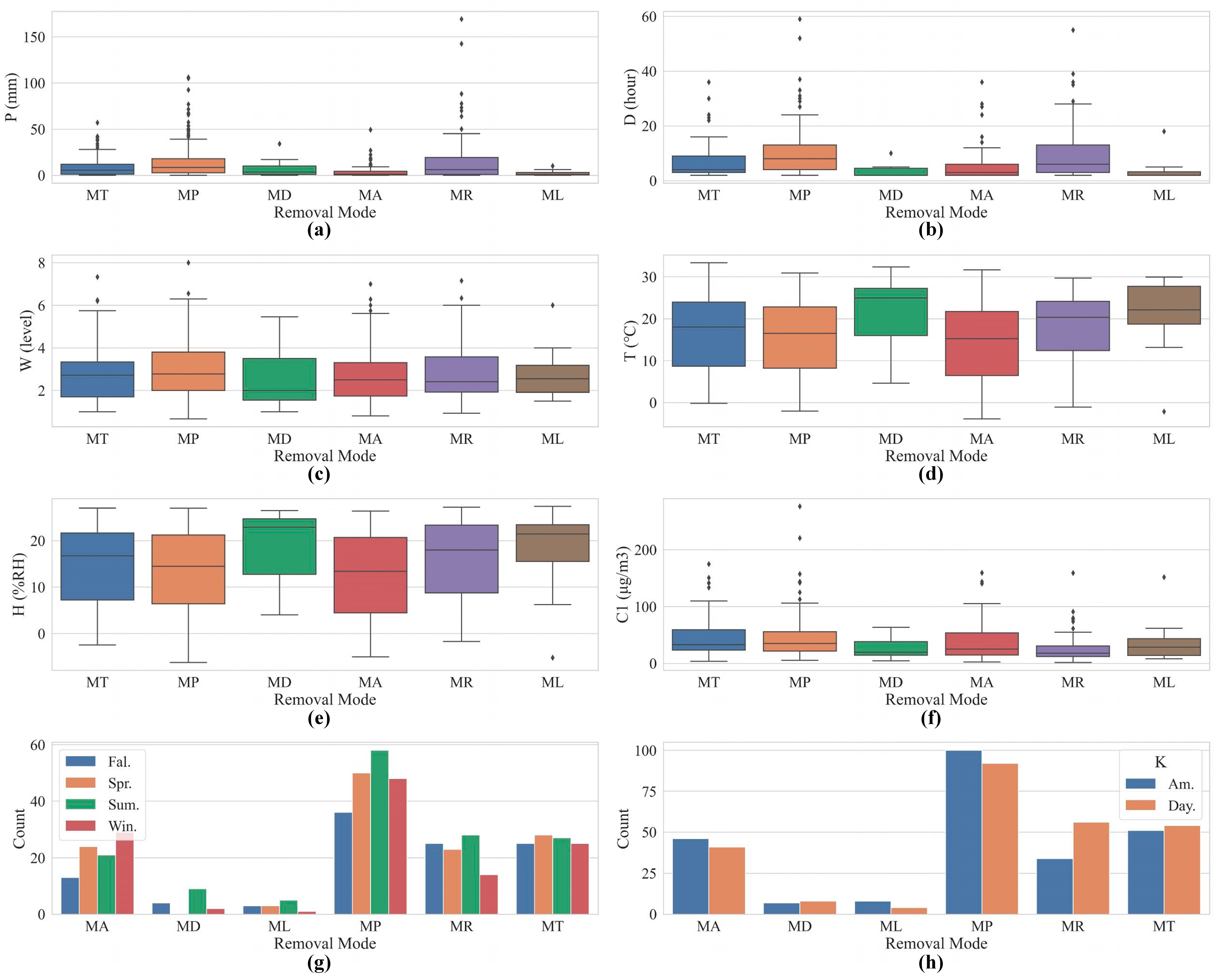
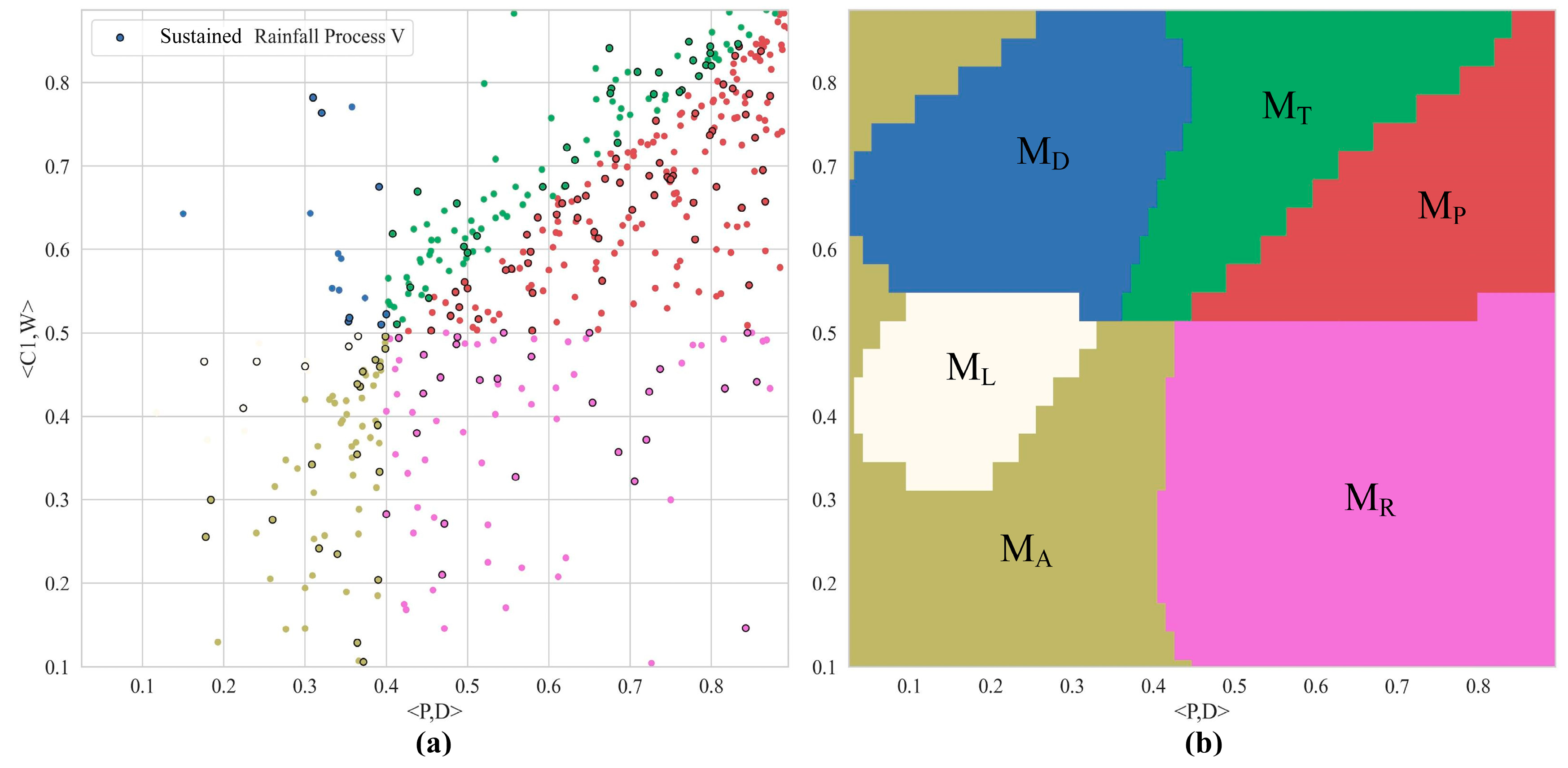
4.2. Principal Component Analysis of the Removal Mode

Due to the large differences in the values of the effectors, the rainfall samples were first normalized by the eigenvector V , and the high-dimensional feature samples of each type of mode were further subjected to the principal component analysis. According to the criteria for selecting the principal components, in this case, when the eigenvalues of the components were all greater than 1 and the cumulative contribution rate was 85%, there were the four types of extracted components. The results are shown in Table 5.
Based on the principal component eigenvalues and variance contribution rates, the factor strengths of different modes were calculated Equation (16) and the strengths of the effectors were ranked, and the total rainfall P , rainfall duration D , initial PM2.5 concentration C 1 and wind speed scale W were selected to participate in the construction of the mode classifier (Table 6).

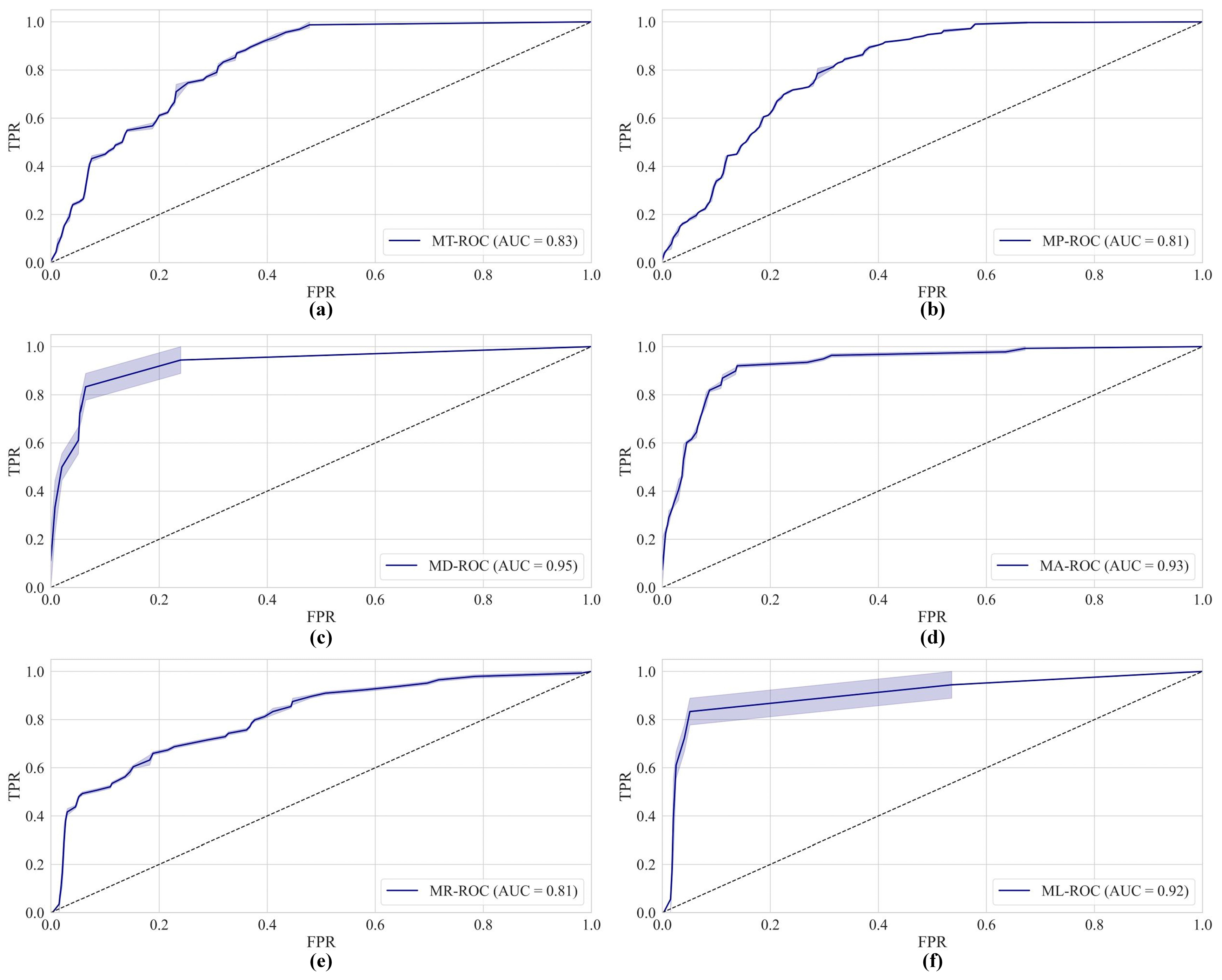
4.3. Predict the Removal Mode and Phenomenon

We combine the above removal concomitant factor strengths with the factorization machines in Section 3.2.4 to build a classifier for predicting the removal mode and phenomenon: the total rainfall P, rainfall duration D, initial PM2.5 concentration C 1 and wind speed scale W in D a t a t r a i n form the feature vector X and the classifier y ^ in Equation (17), and the loss function in Equation (18) is combined to train the classifier according to the stochastic gradient descent (SGD) method. Figure 7 shows the effect of the removal modes classification, where 〈 C 1 , , W 〉 and 〈 P , D 〉 are the factors that form the modal length of the vector, which is used to present the modes distribution based on the effector features; the classifier designed in this paper can classify the sustained precipitation process into the six types described according to the effectors.
To validate the removal effect classifier, all of the sustained rainfall extracted from January 2020 to December of the same year in Nanjing were classified using the samples in D a t a t e s t , and the accuracy of the classification results was evaluated by plotting the receiver operating characteristic (ROC) curve and the curve area, area under the curve (AUC), to evaluate the accuracy of the classification results (Figure 8), where the true positive rate (TPR) and false positive rate (FPR) of the tested samples were calculated as follows:
{ T P R = T P T P + F N F P R = T P F P + T N

5. Discussion

In this paper, we mainly analyze the effect of sustained rainfall on PM2.5 removal from the perspective of a microscopic temporal scale with historical observation data at the hourly scale. By combining previous research results, we propose a model analysis framework to quantitatively describe the removal effect from a more refined perspective for combining the mechanism of sustained rainfall effect on PM2.5. The primary conclusions are summarized as follows.
In this paper, we use hourly scale observations for proposing models to quantitatively express sustained rainfall processes with intermittent duration and relative complexity. It is able to provide data boundaries for studying the role of rainfall removal. Moreover, we consider a large number of environmental influences and construct a concomitant factor model F, which can improve the accuracy and information dimension of the analysis. Based on the above considerations, we conclusively propose the removal modes for a quantitative description of the removal phenomenon.
  • M T 
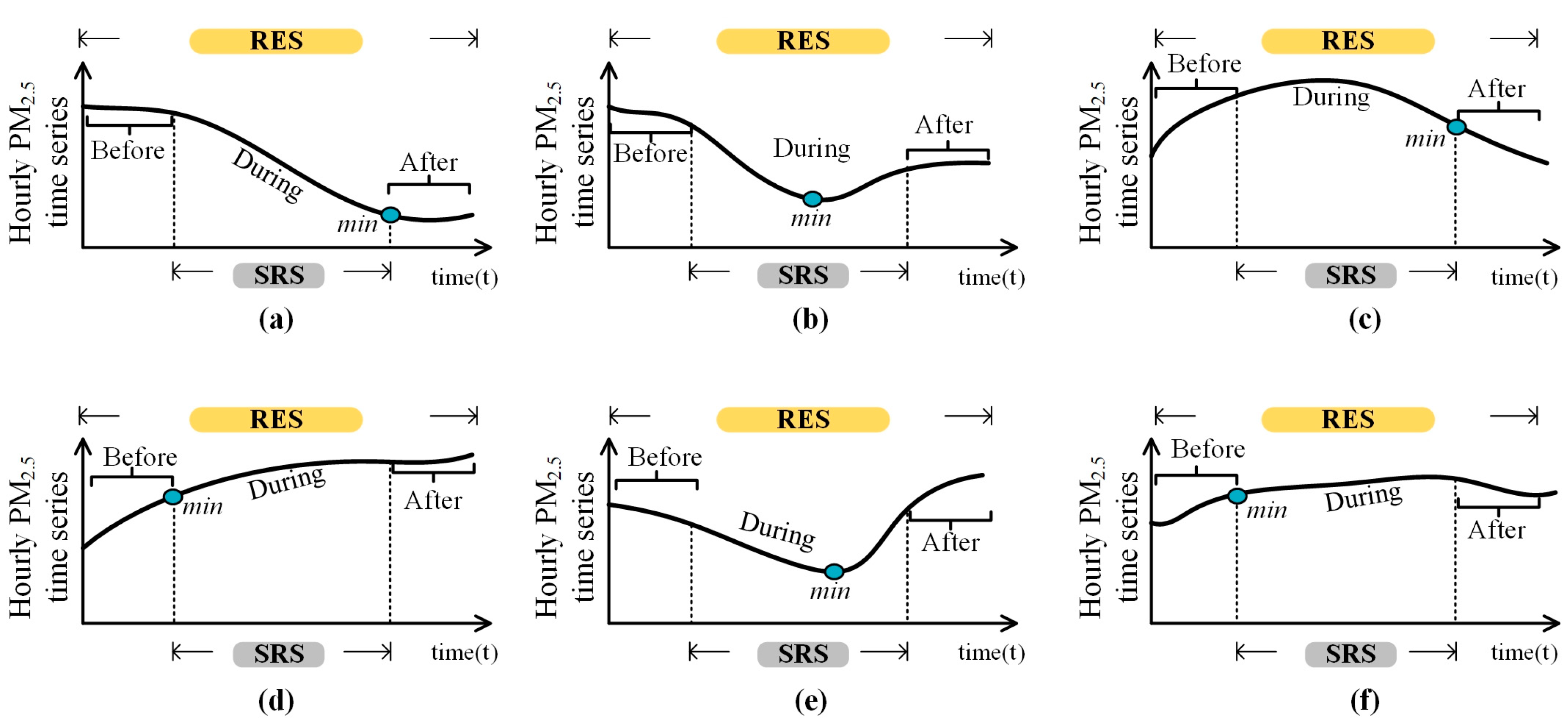
, the PM2.5 concentration change has a continuous decreasing trend during the rainfall process, which has good improvement of the air quality for a period of time after the precipitation.
  • M P , the PM2.5 concentration change is due to the fact that when the removal of particulate pollutants by prolonged precipitation reaches its limit [29], a small portion of the particulate matter does not completely settle to the ground and floats into the air again, thus showing a slight rebound of the concentration values.
  • M D , PM2.5 concentrations continue to rise during rainfall, but drop sharply after the end and are lower than the average concentration values before it.
  • M A , PM2.5 concentration changes in a continuous upward trend when the rainfall duration is too short or small; the humid air will make the suspended pollutants expand, which is more likely to cause the accumulation of pollutants and make the PM2.5 concentration rise.
  • M R , due to the longer duration of the process, there is often a short gap or the secondary precipitation is weak precipitation and other phenomena, which will cause a serious concentration rebound, making the concentration of particulate matter higher than before the precipitation.
  • ML, PM2.5 concentrations continue to rise without rebound during rainfall, and the rise tends to scale off after the end, eventually making the PM2.5 concentrations rise.
The method in this paper is able to classify the proposed model by historical observation data. The results show that of the sustained rainfall processes occurring in Nanjing from 2016 to 2020, only 85 were able to provide complete removal of PM2.5, 63.4% of the precipitation processes resulted in PM2.5 rebound and up to 177 sustained rainfall processes ultimately led to elevated PM2.5 concentrations.
Based on the above quantitative modeling framework, we construct a classifier in combination with the model identification method, considering it for the accurate forecasting of future air quality in short periods. The accuracy evaluation results of the model show that the ROC of our constructed classifier performs well, and the AUC refers to more than 0.85, showing the reasonableness and effectiveness of the method in this paper.
Due to the limited data acquisition, more years of hourly and environmental data for PM2.5 are lacking in this paper. Therefore, it lacks the samples of the lasting ascent mode and the delayed removal mode. Future studies are expected to obtain more hourly temporal observations for the purpose of removal modes construction and acquisition, ultimately to improve the accuracy of the prediction classifiers.

6. Conclusions

Rainfall is an effective way to remove major air pollutants such as PM2.5. However, most studies on the relationship between rainfall data and PM2.5 concentrations have only focused on the changes in the air quality under the influence of long-time span rainfall, ignoring the effects of single rainfall processes that lead to increases or rebound changes in the PM2.5 concentrations, in addition to the effect of wet deposition.
Therefore, based on the definition and generalization of the sustained rainfall process and its effects, this paper uses a time-series statistical method to extract and calculate the single sustained rainfall process and its removal effect factors based on microscopic time-scale observation data; in this process, the effect evaluation index is specifically proposed to quantitatively describe the degree of the removal effect, so as to establish a time-series effect model of PM2.5 concentration removal by rainfall. The potential, deep-seated effect of rainfall processes on PM2.5 concentrations is explored. The model is further combined with pattern recognition theory to design an effect pattern classifier for the sample characteristics of the rainfall process, and finally realize the micro-temporal prediction of air quality after a single rainfall. Using the hourly observation data of Nanjing from 2016 to 2020, a total of 427 sustained rainfall processes were collected using this micro-temporal time-series effects model, and the rate of process, rate of rebound and rate of final were calculated and classified into six types of modes: 85 totally removal mode, 191 partly removal mode, 14 delayed removal mode, 85 rebounding sscend mode and 12 lasting ascent mode. The classifier was constructed based on the factors, indicators and model categories, and the ROC evaluation index showed that the classifier has good performance and is capable of quantitatively predicting future PM2.5 concentration decreases, increases and rebound effects using easily accessible rainfall and PM2.5 concentration forecast information, with a view to providing decision-making information for future regional ambient air quality forecasting and refined control. For the acquisition of hour-by-hour PM2.5 concentration forecasts, further investigation of the finer variation characteristics within rainfall periods is required on the basis of this study.

Author Contributions

Conceptualization, X.X.; methodology, X.X. and T.W.; software, T.W.; validation, T.W. and X.X.; formal analysis, X.X. and T.W.; investigation, T.W.; resources, X.X.; data curation, B.X.; writing—original draft preparation, T.W. and X.X.; writing—review and editing, X.X. and T.W.; visualization, T.W.; supervision, X.X. and T.L.; project administration, B.X.; funding acquisition, B.X. All authors have read and agreed to the published version of the manuscript.

Funding

This research was funded by National Natural Science Foundation of China (41971166) and LZJTU EP (201806).

Institutional Review Board Statement

Ethical review and approval were waived because necessary permissions were obtained from the local governments to which the schools are affiliated for this study. Informed Consent Statement: Informed consent was obtained from all subjects involved in the study.

Informed Consent Statement

Studies not involving human (Not applicable).

Data Availability Statement

Data available on request due to ethical restrictions. The data presented in this study are available on request from the corresponding author. The data are not publicly available due to not having participants consent to share their anonymized data with a third party.

Acknowledgments

We express our sincere appreciation to Qing Zhu from the Faculty of Geosciences and Environmental Engineering, Southwest Jiaotong University and the anonymous reviewer for their constructive comments.

Conflicts of Interest

The authors declare no conflict of interest. The funders had no role in the design of the study; in the collection, analyses, or interpretation of data; in the writing of the manuscript, or in the decision to publish the results.

References

  1. Wu, H.; Gao, X. Multimodal Data Based Regression to Monitor Air Pollutant Emission in Factories. Sustainability 2021, 13, 2663. [Google Scholar] [CrossRef]
  2. Wang, Z.; Liang, L.; Wang, X. Spatiotemporal evolution of PM2.5 concentrations in urban agglomerations of China. J. Geogr. Sci. 2021, 31, 878–898. [Google Scholar] [CrossRef]
  3. Pui, D.; Chen, S.C.; Zuo, Z. PM2.5 in China: Measurements, sources, visibility and health effects, and mitigation. Particuology 2014, 13, 1–26. [Google Scholar] [CrossRef]
  4. Amrita, T. Study of Ambient Air Quality Trends and Analysis of Contributing Factors in Bengaluru, India. Orient. J. Chem. 2017, 33, 1051–1056. [Google Scholar]
  5. Kao, Y.H.; Lin, C.W.; Chiang, J.K. Predictive Meteorological Factors for Elevated PM2.5 Levels at an Air Monitoring Station Near a Petrochemical Complex in Yunlin County, Taiwan. Open J. Air Pollut. 2019, 8, 1–17. [Google Scholar] [CrossRef] [Green Version]
  6. Preethi, B.; Kripalani, R.H.; Kumar, K.K. Indian summer monsoon rainfall variability in global coupled ocean-atmospheric models. Clim. Dyn. 2010, 35, 1521–1539. [Google Scholar] [CrossRef]
  7. Neal, C.; Reynolds, B.; Neal, M.; Pugh, B.; Hill, L.; Wickham, H. Long-term changes in the water quality of rainfall, cloud water and stream water for moorland, forested and clear-felled catchments at Plynlimon, mid-Wales. Hydrol. Earth Syst. Sci. 1999, 5, 459–476. [Google Scholar] [CrossRef] [Green Version]
  8. Liu, Z.; Shen, L.; Yan, C.; Du, J.; Li, Y.; Zhao, H. Analysis of the Influence of Precipitation and Wind on PM2.5 and PM10 in the Atmosphere. Adv. Meteorol. 2020, 2020, 1–13. [Google Scholar] [CrossRef]
  9. Yamamoto, T.; Hori, K.; Tatebayashi, J. An experimental investigation of the PM adhesion characteristics in a fluidized bed type PM removal device. Powder Technol. 2016, 289, 31–36. [Google Scholar] [CrossRef]
  10. Qin, S.; Liu, F.; Wang, J.; Sun, B. Analysis and forecasting of the particulate matter (PM) concentration levels over four major cities of China using hybrid models. Atmos. Environ. 2014, 98, 665–675. [Google Scholar] [CrossRef]
  11. Fu, S.M.; Sun, J.H.; Ling, J.; Wang, H.J.; Zhang, Y.C. Scale interactions in sustaining persistent torrential rainfall events during the Mei-yu season. J. Geophys. Res. Atmos. 2016, 121, 12856–12876. [Google Scholar] [CrossRef]
  12. Liu, Z.Z.; Yan, Z.X.; Duan, J.; Qiu, Z.H. Infiltration regulation and stability analysis of soil slope under sustained and small intensity rainfall. J. Cent. South Univ. 2013, 20, 2519–2527. [Google Scholar] [CrossRef]
  13. Das, A.V.; Basu, S. Temporal trend of microsporidial keratoconjunctivitis and correlation with environmental and air pollution factors in India. Indian J. Ophthalmol. 2021, 69, 1089. [Google Scholar]
  14. Sharma, R.C.; Sharma, N. Statistical Investigation of Effect of Rainfall on Air Pollutants in the Atmosphere, Haryana State, Northern India. Am. J. Environ. Prot. 2018, 6, 14–21. [Google Scholar]
  15. Shaibu, V.O.; Weli, V.E. Relationship between PM2.5 and Climate Variability in Niger Delta, Nigeria. Am. J. Environ. Prot. 2017, 5, 20–24. [Google Scholar] [CrossRef]
  16. Jassim, M.S.; Coskuner, G.; Munir, S. Temporal analysis of air pollution and its relationship with meteorological parameters in Bahrain. Arab. J. Geosci. 2018, 11, 1–15. [Google Scholar] [CrossRef]
  17. Witkowska, A.; Lewandowska, A.U. Water soluble organic carbon in aerosols (PM1, PM2.5, PM10) and various precipitation forms (rain, snow, mixed) over the southern Baltic Sea station. Sci. Total Environ. 2016, 573, 337–346. [Google Scholar] [CrossRef]
  18. Wei, L.A.; Yza, B.; Ping, L.C. Numerical simulation of the influence of major meteorological elements on the concentration of air pollutants during rainfall over Sichuan Basin of China. Atmos. Pollut. Res. 2020, 11, 2036–2048. [Google Scholar]
  19. Kapwata, T.; Wright, C.Y.; du Preez, D.J.; Kunene, Z.; Mathee, A.; Ikeda, T.; Landmandi, W.; Maharajj, R.; Sweijdk, N.; Minakawa, N.; et al. Exploring rural hospital admissions for diarrhoeal disease, malaria, pneumonia, and asthma in relation to temperature, rainfall and air pollution using wavelet transform analysis. Sci. Total Environ. 2021, 2021, 148207. [Google Scholar]
  20. Zhu, T.; Shang, J.; Zhao, D.F. The roles of heterogeneous chemical processes in the formation of an air pollution complex and gray haze. Sci. China-Chem. 2011, 54, 145–153. [Google Scholar] [CrossRef]
  21. Liu, F.; Tan, Q.; Jiang, X.; Yang, F.; Jiang, W. Effects of relative humidity and PM2.5 chemical compositions on visibility impairment in Chengdu, China. J. Environ. Sci. 2019, 86, 15–23. [Google Scholar] [CrossRef]
  22. Guan, P.; Zhang, H.; Zhang, Z.; Chen, H.; Li, Y. Assessment of Emission Reduction and Meteorological Change in PM2.5 and Transport Flux in Typical Cities Cluster during 2013–2017. Sustainability 2021, 13, 5685. [Google Scholar] [CrossRef]
  23. Zhang, C.; Pei, H.; Jia, Y.; Bi, Y.; Lei, G. Effects of air quality and vegetation on algal bloom early warning systems in large lakes in the middle–lower Yangtze River basin. Environ. Pollut. 2021, 2012, 117455. [Google Scholar] [CrossRef]
  24. Amelija, D.; Nenad, Z.; Emina, M.; Jasmina, R.; Miomir, R.; Ljiljana, Z. The effect of pollutant emission from district heating systems on the correlation between air quality and health risk. Therm. Sci. 2011, 15, 293–310. [Google Scholar] [CrossRef]
  25. Li, Y.; Zhu, K. Spatial dependence and heterogeneity in the location processes of new high-tech firms in Nanjing, China. Pap. Reg. Sci. 2017, 96, 519–536. [Google Scholar] [CrossRef]
  26. Zhai, K.; Gao, X.; Zhang, Y.; Wu, M. Perceived Sustainable Urbanization Based on Geographically Hierarchical Data Structures in Nanjing, China. Sustainability 2019, 11, 2289. [Google Scholar] [CrossRef] [Green Version]
  27. Chen, K.; Yan, Y.; Hu, Z. Influence of Air Pollutants on Fog Formation in Urban Environment of Nanjing, China. Procedia Eng. 2011, 24, 654–657. [Google Scholar] [CrossRef] [Green Version]
  28. Wang, G.; Huang, L.; Gao, S.; Song, T. Characterization of water-soluble species of PM10 and PM2.5 aerosols in urban area in nanjing, china. Atmos. Environ. 2002, 36, 1299–1307. [Google Scholar] [CrossRef]
  29. Chen, T.; He, J.; Lu, X.; She, J.; Guan, Z. Spatial and temporal variations of PM2.5 and its relation to meteorological factors in the urban area of nanjing, china. Int. J. Environ. Res. Public Health 2016, 13, 921. [Google Scholar] [CrossRef]
  30. Zou, X.; Qian, Y.; Zhang, S. Spatiotemporal Variations of PM2.5 Concentration and Relationship with Other Criteria Pollutants in Nanjing, China. Nat. Environ. Pollut. Technol. 2018, 17, 499–505. [Google Scholar]
  31. Guijo-Rubio, D.; Duran-Rosal, A.M.; Gutierrez, P.A.; Troncoso, A.; Hervas, M.C. Time-Series Clustering Based on the Characterization of Segment Typologies. IEEE Trans. Cybern. 2020, 99, 1–14. [Google Scholar] [CrossRef] [PubMed]
  32. Leles, M.C.; Sansão, J.P.H.; Mozelli, L.A.; Guimarães, H.N. Improving reconstruction of time-series based in singular spectrum analysis: A segmentation approach. Digit. Signal Process. 2017, 77, 63–76. [Google Scholar] [CrossRef]
  33. Onuorah, C.U.; Leton, T.G.; Momoh, Y. Influence of meteorological parameters on particle pollution (PM2.5 and PM10) in the tropical climate of port harcourt, nigeria. Arch. Curr. Res. Int. 2019, 1–12. [Google Scholar] [CrossRef]
  34. Kayes, I.; Shahriar, S.A.; Hasan, K.; Akhter, M.; Salam, M.A. The relationships between meteorological parameters and air pollutants in an urban environment. Glob. J. Environ. Sci. Manag. 2019, 5, 265–278. [Google Scholar]
  35. Uchiyama, R.; Okochi, H.; Ogata, H.; Katsumi, N.; Nakano, T. Characteristics of trace metal concentration and stable isotopic composition of hydrogen and oxygen in “urban-induced heavy rainfall” in downtown Tokyo, Japan; the implication of mineral/dust particles on the formation of summer heavy rainfall. Atmos. Res. 2018, 217, 73–80. [Google Scholar] [CrossRef]
  36. Gautam, S.; Yadav, A.; Pillarisetti, A.; Smith, K.; Arora, N. Short-term introduction of air pollutants from fireworks during diwali in Rural Palwal, Haryana, India: A case study. IOP Conf. Ser.: Earth Environ. Sci. 2018, 120, 012009. [Google Scholar] [CrossRef]
  37. Yang, W.; He, Z.; Huang, H.; Huang, J. A clustering framework to reveal the structural effect mechanisms of natural and social factors on PM2.5 concentrations in China. Sustainability 2021, 13, 1428. [Google Scholar] [CrossRef]
  38. Kashki, A.; Karami, M.; Zandi, R.; Roki, Z. Evaluation of the effect of geographical parameters on the formation of the land surface temperature by applying ols and gwr, a case study shiraz city, Iran. Urban Clim. 2021, 37, 100832. [Google Scholar] [CrossRef]
  39. Zhang, Y.; Zhang, F.; Zhu, H.; Guo, P. An optimization-evaluation agricultural water planning approach based on interval linear fractional bi-level programming and iahp-topsis. Water 2019, 11, 1094. [Google Scholar] [CrossRef] [Green Version]
  40. Kulanuwat, L.; Chantrapornchai, C.; Maleewong, M.; Wongchaisuwat, P.; Boonya-Aroonnet, S. Anomaly detection using a sliding window technique and data imputation with machine learning for hydrological time series. Water 2021, 13, 1862. [Google Scholar] [CrossRef]
  41. Cai, T.T.; Ma, Z.; Wu, Y. Sparse pca: Optimal rates and adaptive estimation. Ann. Stat. 2012, 41, 3074–3110. [Google Scholar] [CrossRef]
  42. Wang, S.; Li, C.; Zhao, K.; Chen, H. Learning to context-aware recommend with hierarchical factorization machines. Inf. Sci. 2017, 409–410, 121–138. [Google Scholar] [CrossRef]
Figure 1. Macro/micro-temporal scale of sustained rainfall-PM2.5 observation data series and removal phenomenon in Nanjing from 2016 to 2020: (a) Yearly temporal-level; (b) Monthly temporal-level; (c,d) Hourly temporal-level.
Sustainability 13 11022 g001
Figure 2. Schematic diagram of a micro-temporal model of the sustained rainfall process.
Sustainability 13 11022 g002
Figure 3. Schematic diagram of a micro-temporal model of the removal effects process and concomitant factor.
Sustainability 13 11022 g003
Figure 4. Schematic diagram of the sustained rainfall-PM2.5 removal modes. (a) Totally Removal Mode; (b) Partly Removal Mode; (c) Delayed Removal Mode; (d) Totally Ascent Mode; (e) Rebounding Ascend Mode; (f) Lasting Ascent Mode.
Sustainability 13 11022 g004
Figure 5. Flowchart for the prediction of sustained rainfall-PM2.5 removal effect using the quantitative model.
Sustainability 13 11022 g005
Figure 6. Distribution of the numerical distribution of concomitant factors for different removal modes. (a) Rainfall Total P and removal modes; (b) Rainfall Duration D and removal modes; (c) Wind Power W and removal modes; (d) Temperature T ¯ and removal modes; (e) Humidity H ¯ and removal modes; (f) Initial PM2.5  C 1 and removal modes; (g) Seasonal factor S and removal modes; (h) Day and night factor K and removal modes.
Sustainability 13 11022 g006
Figure 7. FM classifier result graph for removal modes, (a) Scatter plot of modes classification results; (b) Interpolated rendering of modes classification results.
Sustainability 13 11022 g007
Figure 8. The ROC and AUC of removal modes classifier, (a) ROC of Totally Removal Mode; (b) ROC of Removal Mode; (c) ROC of Delayed Removal Mode; (d) ROC of Totally Ascend Mode; (e) ROC of Rebounding Ascend Mode; (f) ROC of Lasting Ascend Mode.
Sustainability 13 11022 g008
Table 1. Table of qualitative descriptions of concomitant factor.
ClassFactorLabelImpact Effects
FFDRainfall Total P High correlation with air pollutant concentrations, which can directly influence the removal effect
Rainfall Duration D
FITemperature T ¯ When the temperature near the ground is high, atmospheric convection is intensified, which tends to reduce PM2.5 concentrations, and conversely PM2.5 is not easily dispersed
Humidity H ¯ Changes in PM2.5 are closely related to the moisture content of the air, with "hygroscopic increase" occurring due to the adsorption of particulate matter concentrations
Wind Power W Stronger winds also facilitate the dilution and uplift of pollutants
Initial PM2.5 C 1 The effect of removal is influenced by the magnitude of PM2.5 concentrations before rainfall, and has little effect on particulate concentrations when air quality is good
Seasonal S The removal effect is mostly higher at night than during the day; the total positive removal of sustained rainfall will be slightly higher in autumn than in other seasons
Day and night K
Table 2. Table of sustained rainfall-PM2.5 removal modes, quantitative classification and qualitative description.
Removal   Mode   M i Effect IndicatorsTrends in PM2.5 Concentrations
R P   R S   R R   DuringAfterMin
M T >0<0>0Continued declineDeclineNon-existent
M P >0>0>0Decline, reboundDeclineExistent
M D <0<0>0Continued riseDeclineExistent
M A <0>0<0Continued riseRiseNon-existent
M R >0>0<0Decline, reboundRiseExistent
M L <0<0<0Continued riseRiseExistent
Table 3. Table of quantitative calculation of concomitant factor.
FClassLabelTime-Series RangeQuantitative Calculation
FD P S R S P = t = t t R t   (3)
D D = t = t t t (4)
FI T ¯ T ¯ = t = t t T t t t (5)
H ¯ H ¯ = t = t t H t t t (6)
W W { 0 , 1 , , 17 } (7)
C 1 R E S C 1 = t = ( t n ) t C t n (8)
S S R S S { S p r , S u m , F a l , W i n } (9)
K K { A m , P m } (10)
Table 4. A sample table of the sustained rainfall time series in Nanjing.
V [ t n , t + n ] P D T ¯ H ¯ W C 1 S K [ R F , R S , R P ]   M
V 1 2016/01/04/18:00-2016/01/05/07:0018.0128.214.914276.3342[0.96, 0.31, 0.95] M P
V 2 2016/01/10/21:00-2016/01/11/08:007.0126.043.673150.6742[0.19, −0.03, 0.22] M T
……………………
V 426 2020/10/15/16:00-2016/10/16/17:0017.62414.022.31215.3332[0.93, 0.83, 0.61] M P
V 427 2020/10/21/05:00-2020/10/21/10:003.8617.384.75238.3330[0.08, −0.02, 0.11] M T
Table 5. Explanatory table for the principal component analysis of removal mode.
Component Eigenvalue   ( λ ) Contribution   of   Variance   E ( λ ) Cumulative Contribution (%)
Principal component 12.77435.6735.67
Principal component 22.10127.5663.26
Principal component 31.66216.2879.54
Principal component 41.07911.4691.00
Principal component 50.6626.06197.06
Principal component 60.1562.94100.00
Table 6. Concomitant factor intensity of the sustained rainfall time series sample with removal mode.
M T M P M D M A M R M L
P 0.2230.3390.2320.2500.3060.421
D 0.2140.2940.4530.3210.2760.559
T ¯ 0.1270.168−0.045−0.174−0.164−0.103
H ¯ 0.0790.176−0.137−0.076−0.0370.218
W 0.2630.1320.2320.2710.3860.372
C 1 0.1930.2660.4110.2630.4420.421
S 0.0740.1350.0330.173−0.1540.032
K 0.0310.0950.1270.041−0.0760.093
Publisher’s Note: MDPI stays neutral with regard to jurisdictional claims in published maps and institutional affiliations.

