Are Tourism and Energy Consumption Linked? Evidence from Australia

Abstract

Tourism contributes to the growth of an economy via earning foreign currencies and employment opportunities. However, tourism also contributes to greater energy consumption because of various tourist activities such as hotel accommodations and transportation. This study investigates the long-term cointegrating relationship between international tourist arrivals and primary energy consumption in Australia. In addition, the roles of gross domestic product, gross fixed capital formation, financial development, and total population on energy consumption are also examined. The study covered the last four decades (1976–2018) using data from the Australian Bureau of Statistics, BP Statistical Review, and the World Development Indicators. Augmented Dickey-Fuller, Phillips-Perron, Autoregressive distributed lag (ARDL) bound tests, Johansen and Juselius, Bayer-Hanck cointegration test, and several key diagnostic tests have been conducted to assess the relationship. The estimated results indicate that tourist arrivals, gross domestic product, and financial development have a significant long-run cointegrating relationship with energy consumption. Policy measures are suggested based on the findings of this study.

1. Introduction

Tourism is regarded among the most prominent of the service sectors and vital global industry. According to the World Travel and Tourism Council [1], in 2019, the tourism industry was responsible for creating 330 million jobs worldwide and contributed US$8.9 trillion to the world’s gross domestic product (GDP), representing 10.3% of the global GDP. Tourism helps create jobs, partly due to tourists arrival, generate revenues (e.g., earnings from foreign currencies), and eventually [2] impacts the economic growth of a country, including during the period of economic crisis [3,4] The growth in domestic and international tourist arrivals boosts a country’s income while simultaneously leads to the growth in energy consumption, for instance, by increasing tourism activities such as a hotel stay and the use of transportation facilities [5,6,7]. Among these activities, the transportation sector, especially air transportation, significantly contributes to the increase of energy consumption [7], and therefore emission. Thus, the relationship between tourism and energy consumption is a topic of interest for academic researchers and economic policymakers.

Tourism has a negative environmental impact, as found in the case of Greece [8]. Tourism also has both positive and negative effects on the emissions found in different countries [9]. Moreover, China and Turkey have experienced tourism-led growth, while Spain and Russia have enjoyed growth-led tourism [10]. Change in international trade and the changing pattern of globalization have attracted many researchers to examine the relationship among energy, emission and trade in different regions, globalization and energy source [11], and economic growth and energy consumption [12,13] in different regional settings. The impact of tourism and energy on carbon dioxide (CO₂) emission has also been investigated in G7 countries [8]. Empirical studies to test various theories related to tourism are also available in the literature [14,15]. However, there is limited research about the nexus between tourism and energy consumption from a single developed country perspective. Against this backdrop, this research aims to examine the linkage between tourism in Australia and energy consumption.

Recent literature argues that technological innovation, economic condition, urbanization, regional environmental planning, and industrial structure are a few of the factors impacting the tourism industry [16]. Wilson et al. [17] suggested that unless the entrepreneurs involve themselves directly or indirectly, rural tourism would not be flourished. Focusing on entertainment tourism, Luo et al. [18] identified quality of tourism service, logistic support, advertising and security concerns as the success factor. However, the factors vary according to the new directions of tourism development. Some countries are promoting medical tourism, while some countries or regions attract agricultural or rural tourism [19,20]. However, the impact of tourism on national and regional energy consumption is an underexplored area of study.

From a policy perspective, energy consumption has a significant effect on economic growth, as it is the basis for modern industrial societies. Energy provides facilities for household consumption, resource mining, industrial production, and transportation. Thus, development and economic growth cannot be achieved without a more significant use of energy [21]. However, there are serious environmental consequences to high energy consumption [22,23], including the increased concentration of carbon gases (e.g., carbon dioxide emissions) in the atmosphere, resulting in climate change [24,25]. The natural ecosystems that influence economic activity and human wellbeing are diminishing because of climate change. The significant environmental consequences of energy use have increased atmospheric concentrations of greenhouse gases, such as CO₂. In Australia, greenhouse gas emissions continue to be a major issue in the energy sector, rising from 74% of net emissions in 2011 to 76% in 2015 [26]. Moreover, the country has experienced severe natural disasters in recent times (e.g., bushfires, droughts and floods) [27]. In addition, Australia has seen a massive surge in international tourism and energy consumption over the past three decades (see

Table 1. Trend of Tourist Arrivals, Energy Consumption and GDP in Australia.

Year	EC	TA	GDPPC	GFCF	TP	FD
1976	192.80	531,900	27,944.23	64,585,780,433.57	14,033,000	27.89
1980	207.31	904,700	29,907.79	78,679,518,637.01	14,692,000	27.88
1985	205.04	1,142,700	32,045.32	99,241,086,962.29	15,758,000	37.10
1990	224.38	2,214,900	35,912.21	126,738,577,854.89	17,065,100	60.68
1995	233.07	3,725,900	38,095.13	137,948,490,238.46	18,072,000	69.95
2000	248.98	4,931,300	44,334.39	187,230,705,595.27	19,153,000	87.73
2005	250.74	5,463,000	48,813.89	244,248,599,456.41	20,394,800	108.79
2010	248.14	5,871,600	52,022.13	310,545,230,335.59	22,031,750	125.49
2015	243.89	7,449,900	55,079.90	349,074,648,712.05	23,815,995	136.31
2018	240.81	9,245,800	56,864.30	353,055,394,684.73	24,982,688	139.42

Note: Presents data for the selected number of years to avoid a large size table. EC = primary energy consumption in gigajoule per capita; TA = international tourism number of arrivals; GDPPC = GDP per capita (constant 2010 US$); GFCF = gross fixed capital formation (constant 2010 US$); TP = total population; FD = financial development as % of GDP.

).

Australia welcomed 9.2 million international tourists in 2018, representing more than one-third of the country’s population. However, no empirical research has examined the long-run cointegration relationship between international tourist arrivals and energy consumption in Australia. Without understanding the crucial effect of tourism (one of Australia’s major economic activities) on energy consumption, it is improbable that the Australian government will devise policies to reduce tourism-related carbon emissions. Consequently, this study’s primary objective is to examine the long-run cointegration relationship between tourist arrivals and energy consumption in Australia. The secondary aim is to estimate the effect of tourist arrivals on energy consumption while holding other key variables constant (e.g., economic growth, energy consumption, foreign direct investment, capital, financial development and total population). The findings will help policymakers of both Australia and other countries. Given that the carbon emissions or environmental pollution related to tourism activities depend on the source of energy (e.g., renewable or non-renewable) [5], the outcomes will also indicate whether Australia’s tourism industry should take measures to improve energy efficiency and productivity. The findings will also signify whether energy-efficient technologies may be implemented in tourism-related activities to decrease energy consumption. However, it has to be noted that the exact relevance of this research findings would be subject to the presence of COVID-19.

The spread of COVID-19 has impacted the tourism industry substantially globally [28]. A sharp decline in international air traffic, empty sea-beaches, and football matches without spectators are the visible indications. Moreover, mandatory vaccination is not acceptable to all, and inadequate or false information about COVID related rules and regulations also impact the industry [29]. However, after the COVID-19 pandemic, the world is likely to witness a considerable rise in tourism growth, which could help nations recover from economic crises. Hence, a study combining tourism and energy consumption has the potential to address the national development aspects of a country such as Australia and also has the prospect to be used as background information in shaping national policies focusing on the Paris Agreement.

2. Tourism, Energy Consumption, and GDP in Australia

Australia became a popular tourist destination during the 1970s and 1980s. Table 1 presents Australia’s number of tourist arrivals, energy consumption and economic growth from 1976 to 2018. During the period, the number of international tourist arrivals increased from 531,900 to 904,700. The original Crocodile Dundee film paved the way for Australia to be included on the tourism map for Americans [30]. The surge in tourism during the 1980s progressed regarding the extent, position and significance of tourism in Australia [31]. Australia’s tourism industry experienced growth in the number of tourist arrivals in the 1990s, resulting in tourism being the largest earner of foreign currency during this time [32]. During the 2000 Sydney Olympic Games, the number of arrivals skyrocketed to nearly half a million. This number steadily gained increasing momentum until 2018.

Australia’s primary energy consumption shows an upwards trend of per capita energy use from 1976 to 1995, increasing from 192.80 to 233.07 gigajoules of energy consumption. In the 2000s, primary energy consumption abruptly increased to 2535.01 gigajoules per capita. One reason for this increase was the 2000 Sydney Olympics, which directly affected electricity demand and consumption [33]. After 2005, a downwards movement of energy use was seen in Australia. Furthermore, Ryan et al. [34] demonstrated that Australian primary energy consumption has declined since 2008. Improved appliance efficiency and fuel switching are significant causes of such decline in energy use [34]. However, Ryan et al. [34] projected that this decline will continue only until the 2020s and then will increase, as no new regulatory-driven changes will occur to drive further significant energy efficiency improvement.

The trend of economic growth in Australia’s economy, as seen in Table 1, shows that per capita GDP was US$27,944.23 and US$29,907.79 in 1976 and 1980, respectively. There was a steady rise in GDP from 1985 to 1995. In 2000, the growth was more than 14% compared with the growth observed in 1995, and GDP reached US$44,334.39 per capita. Each year from 2005 to 2018 also showed an increasing GDP trend in the Australian economy. 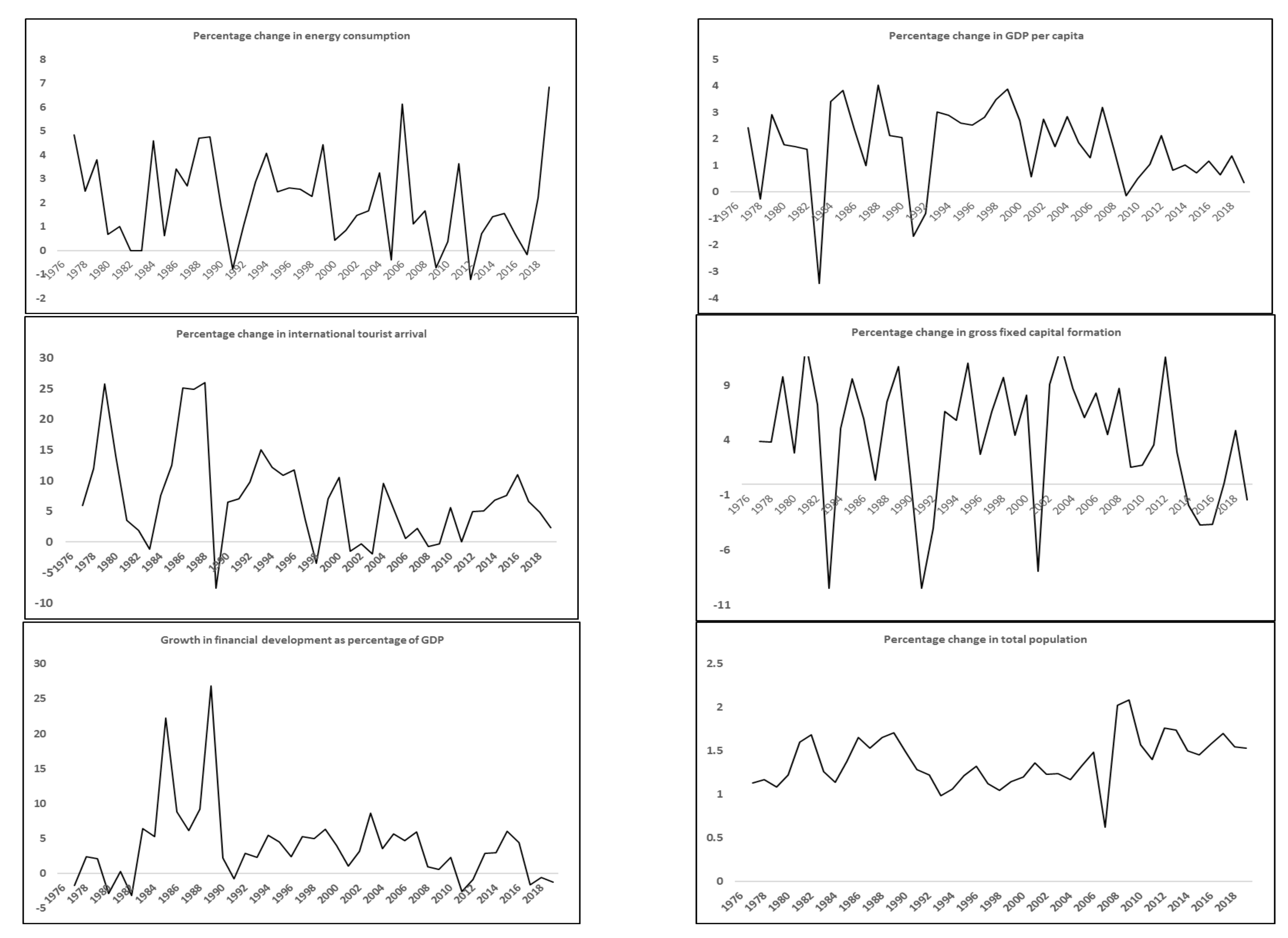Figure 1 presents the trend for the log forms of all variables from 1977 to 2018. Logarithms were chosen to obtain a more stable variance [35]. It is clear that the variables displayed no linear trend, and none had an evident seasonality.

3. Literature Review

The existing literature on energy economics generally focuses on the link between economic growth, energy, tourism, and carbon emissions [36,37,38,39,40,41,42,43,44,45,46]. The nexus between tourism and energy has been a neglected topic, with a relatively smaller strand of literature studying the relationship between energy consumption and the tourism sector ignoring CO₂ [47,48,49]. Tourism is considered one of the biggest drivers of economic growth for many countries. Energy consumption creates a crucial connection between tourism and environmental quality, as pollution and greenhouse gas emissions are mainly caused by energy consumption [41]. Zhang et al. [46] explored the effects of international tourism on China’s economic growth, energy consumption and carbon emissions using panel data between 1995 and 2011, based on the environmental Kuznets curve (EKC) hypothesis and panel cointegration modeling techniques. Their estimated outcomes indicated that tourism causally affects economic growth and CO₂ emissions in China’s eastern, western and central regions.

In the same way, in the Malaysian context, Solarin [50] investigated the determinants of CO₂ emissions, emphasizing tourism development from 1972 and 2010, and found a short-run unidirectional causality running from tourism to energy consumption. These findings were further supported by Alola et al. [51], who found a unidirectional relationship between tourist arrivals and energy consumption in 16 coastline Mediterranean countries between 1995 and 2014. In another research, Katircioglu et al. [39] argued that a 1% change in tourism resulted in a 0.033% change in CO₂, and the effect was more remarkable for energy consumption with a 0.619% change. The study based its analysis on autoregressive distributed lag (ARDL) and the Granger causality test over data of 39 years. It concluded that tourism had a direct and statistically significant effect on energy consumption in the long term and was a catalyst for energy consumption. Katircioglu [40] estimated the relationship between tourism and energy with impulse responses and variance decomposition analyses. The results showed that energy consumption increased by tourism development predominantly in the longer term.

In another study, the feedback hypothesis used by Ben Jebli et al. [37] supported that there was a short-run Granger causality between development of the economic sectors of touristic zones and energy consumption. The vector error correction model (VECM) results showed a unidirectional long-run causality from energy use to international tourism. A short-run Granger showed a bidirectional causality between them. Tang et al. [52] explored the dynamic causal and inter-relationships among India’s tourism, economic growth, and energy consumption using data from 1971 to 2012. They used the bounds testing approach to cointegration and the Gregory–Hansen test for cointegration with a structural break. The result revealed that economic growth and tourism together explained most of the forecast error variance in energy consumption. However, energy consumption only explained less than 9% of the economic growth and tourism variations. Thus, in the long run, tourism and economic growth strongly affected energy consumption. Ali et al. [53] conducted a study with 19 Asia Cooperation Dialogue member countries using data from 1995 to 2015. They demonstrated that the existence of a feedback hypothesis between renewable energy consumption and tourism for higher-income countries implied that these variables significantly affected each other.

However, using ARDL and Granger causality tests for a developing country, Nepal et al. [43] conducted a study to explore the short-run and long-run relationship between tourist arrivals, per capita economic output, emissions, energy consumption and capital formation in Nepal. Interestingly, they found a unidirectional causality between primary energy consumption and the number of tourist arrivals, where a 1% increase in energy consumption decreased tourist arrivals by 3.84%. This demonstrated that energy consumption negatively affected tourist arrivals because of firewood consumption and lessening dependence on fossil fuels in Nepal in particular and the developing countries in general. Similarly, no causality was found between tourist arrivals and energy consumption in the European Union and the candidate countries [5]. Furthermore, in another panel study, Naradda Gamage et al. [42] examined whether energy consumption and tourism supported the EKC hypothesis. Their investigation revealed that tourism development was not a threat to environmental quality in Sri Lanka in the long run.

In recent years, there has been considerable interest in examining the relationship between tourism and energy consumption. Gokmenoglu et al. [49] investigated the role of international tourism on Turkey’s energy consumption with data spanning 55 years (1960 to 2015). Using Hacker and Hatemi-J’s bootstrap corrected causality results, the key findings indicated unidirectional causality from tourist arrivals to energy consumption. They concluded that international tourism was a significant contributor to energy consumption in Turkey. Similarly, Amin et al. [47] examined the tourism–energy nexus for selected South Asian countries using data from 1995 to 2015. The results indicated unidirectional causality running from tourist arrivals to energy consumption in the long run. Selvanathan et al. [44] too investigated the inter-relationships between tourism, energy consumption, carbon emissions and GDP for South Asian countries. The research applied panel ARDL and VECM frameworks with data from 1990 to 2014 and concluded that tourism positively affected energy consumption in Bangladesh, India, Nepal and Pakistan. However, with increased energy consumption because of tourism development activities in South Asia, there are significant risks for environmental quality through increased CO₂ emissions. Ali et al. [36] inspected the effect of tourist arrivals, structural change, economic growth and energy use on carbon emissions in Pakistan using data from 1981 to 2017. This study employed ARDL, Bayer and Hanck, VECM and the Granger causality test to conclude that increasing tourist arrivals caused a 0.06% increase in CO₂ emissions in the long run. The authors also suggested that tourist arrivals pollute the environment by consuming energy in transportation, accommodation and shopping. A recent study conducted by Shi et al. [54] deduced that over the long term, for upper-middle-income countries, one-way causality ran from tourists’ expenditure per capita and the net inflow of international tourism to primary energy consumption. For the high-income countries panel, unidirectional short-run causality ran from primary energy consumption to inbound tourists’ expenditure per capita. Thus, the results showed that the effects of tourism on energy consumption varied because of income differences in the countries concerned. The paper included the carbon emissions nexus while measuring tourism’s impact on energy consumption. However, a limited number of studies examined the relationship between tourism and energy consumption without carbon emissions. Isik et al. [50] explored the nexus between tourism development, renewable energy consumption and economic growth using panel data from 1995 to 2012. This study used a Lagrange multiplier, panel cointegration test and Emirmahmutoglu-Kose bootstrap Granger causality test. They identified four main results: (i) tourism-led energy was seen in Italy, Spain, Turkey and the United States; (ii) energy-led tourism was seen in China; (iii) two-way causality was seen in a panel of T7 most-visited countries; and (iv) no causality was seen in France and Germany.

Additionally, GDP—usually a proxy for economic growth and energy consumption—is co-dependent with energy use—that is, an increase in energy use causes economic growth to increase, and vice versa [55,56,57,58,59]. Likewise, gross fixed capital formation [60] and financial development [61,62] stimulate energy consumption. An increase in population also increases energy use [63]. There are limited studies on the tourism and energy consumption relationship in the literature, and no empirical evidence exists for Australia. Moreover, there is no cointegration tests for Australia in the literature using large-scale country-specific time-series data regarding the relationship between tourist arrivals, economic growth, energy consumption, capital, financial development and total population. Finally, only limited research has used total population as a control variable to investigate the relationship between tourism and energy consumption. Therefore, this study aimed to fill the omitted variable bias gap. Accordingly, additional variables have been chosen since energy consumption is struck by the volume of national business and agricultural and industrial activities, which in turn impact capital and financial development.

4. Materials and Methods

4.1. Data

The main objective of this study was to investigate the long-run and short-run effects of international tourist arrivals on energy consumption in the Australian context. This study employed annual time-series data for the duration from 1976 to 2018. Data on international tourist arrivals were gathered from the Australian Bureau of Statistics [64], while the other data were collected from the World Development Indicator [65] and BP Statistical Review [66].

Table 2. Variable Description and Data Sources.

Symbol	Variable	Definition	Source
EC	Energy consumption	Primary energy consumption	BP Statistical Review
TA	Tourist arrivals	International tourism, number of arrivals; number of movements; short-term visitors arriving	ABS
GDP	GDP per capita	GDP per capita (constant 2010 US$)	WDI
CAP	Gross fixed capital formation	Gross fixed capital formation (constant 2010 US$)	WDI
TP	Total population	Total population based on de facto definition of population with mid-year estimates	WDI
FD	Financial development	Domestic credit to private sector (% of GDP)	WDI

presents variable descriptions and data sources.

4.2. Econometric Methods

This study built its framework following the study of Amin et al. [47], who investigated the tourism (TA) and energy (EC) nexus with economic growth (GDP) in selected South Asian countries. In addition, this study included capital formation, total population and financial development to avoid omitted variable bias. Gokmenoglu et al. [49] emphasized the importance of population in determining energy use. Omri et al. [67] empirically investigated the relationship between capital formation and FD, and found that capital and FD have a positive and significant effect on EC. The following empirical model was used to test the link between international tourist arrivals and energy consumption in Australia:

LNEC_t = β₀ + β₁ LNTA_t + β₂ LNGDP_t + β₃ LNCAP_t + β₄ LNTP_t + β₅ LNFD_t + ε_t

(1)

where LN is the log form, t indicates time, ε_t denotes the error terms, EC is per capita energy consumption, TA is the number of international tourist arrivals, GDP is per capita GDP, CAP is gross fixed capital formation, TP is total population and FD is financial development as a percentage of total GDP. The initial expectation was that all these variables would positively affect energy consumption. To stabilize the variance of the series, this study used the logarithmic forms of the variable of interest [68].

4.3. Unit Root Test

The stationarity of time-series data is critical, as the causality test outcomes rely on the stationarity of the data and, often, the macroeconomic variables contain a unit root. According to Lütkepohl et al. [35], a stochastic process is termed stationary if it has time-invariant first and second moments. In other words, statistical properties remain constant. In this analysis, the unit root test was based on both the augmented Dickey-Fuller (ADF; [69,70]) and Phillips-Perron (PP; [71]) tests.

If the first difference of a variable is stationary, it is considered to be integrated of order I (1) [70,71]. The following auxiliary equation was used from Lütkepohl et al. [35]:

$$\Delta {\mathrm{y}}_{\mathrm{t}}=\mu +{\propto }_{\mathrm{i}}{\mathrm{y}}_{\mathrm{t}-1}+{{\displaystyle \sum }}_{\mathrm{i}=1}^{\mathrm{k}}{\mathsf{\pi }}_{\mathrm{i}}\Delta {\mathrm{y}}_{\mathrm{t}-\mathrm{i}}+{\mathsf{\epsilon }}_{\mathrm{t}}$$

(2)

where _it is the relevant time-series variable, t indicates the linear deterministic trend, Δ is the first difference operator, ∝_i is the parameter of interest, k is the maximum lag order and ε_t is the error term. If |∝_i | < 1, the series is trend stationery; conversely, when |∝_i| ⩾ 1, the series has the unit root and is thus not stationary [72]. For further details on the time-series unit root test, see Hamilton [73] and Lütkepohl et al. [35]. The PP model tests equations as given below:

$$\Delta {\mathrm{y}}_{\mathrm{t}}={\mathsf{\pi }\mathrm{y}}_{\mathrm{t}-1}+{\mathsf{\beta }}_{\mathrm{i}}{\mathrm{D}}_{\mathrm{t}-\mathrm{i}}+{\mathsf{\epsilon }}_{\mathrm{t}}$$

(3)

where ε_t is a I (0) with zero mean and ${\mathrm{D}}_{\mathrm{t}-\mathrm{i}}$ is a deterministic trend component.

4.4. Cointegration Analysis

A further phase of the analysis was to examine the cointegration among the variables. We checked the existence of the long-run relationship among the variables using three different cointegration techniques: ARDL bound, Johansen cointegration and Bayer-Hanck cointegration tests.

4.5. Bound Testing Technique

This study used the ARDL bound test technique to examine the cointegration between Australia’s energy consumption and other explanatory variables. The ARDL bound test developed by Pesaran et al. [74] provides two asymptotic critical value bounds when the independent variables are either I (0) or I (1). It is assumed that the F-statistic value exceeds the upper critical bound—that is, I (1)—so it can be concluded that there is cointegration between the variables, and a long-run relationship among the variables exists. The ARDL model for the estimations was as follows:

$$\begin{array}{cc}{\mathsf{\Delta }\mathrm{LNEC}}_{\mathrm{t}}=& { \mathsf{\beta }}_0+{ \mathsf{\beta }}_1{\mathrm{LNEC}}_{\mathrm{t}-1}+{\mathsf{\beta }}_2{ \mathrm{LNTA}}_{\mathrm{t}-1}+{ \mathsf{\beta }}_3{ \mathrm{LNGDP}}_{\mathrm{t}-1}+{ \mathsf{\beta }}_4{ \mathrm{LNCAP}}_{\mathrm{t}-1}\\ & +{\mathsf{\beta }}_5{ \mathrm{LNTP}}_{\mathrm{t}-1}+{ \mathsf{\beta }}_6{ \mathrm{LNFD}}_{\mathrm{t}-1}+{{\displaystyle \sum }}_{\mathrm{i}=1}^{\mathrm{p}}{\mathsf{\alpha }}_1{\mathsf{\Delta }\mathrm{LNEC}}_{\mathrm{t}-\mathrm{i}} \\ & +{{\displaystyle \sum }}_{\mathrm{i}=1}^{\mathrm{p}}{\mathsf{\alpha }}_2{\mathsf{\Delta }\mathrm{LNTA}}_{\mathrm{t}-\mathrm{i}}+{{\displaystyle \sum }}_{\mathrm{i}=1}^{\mathrm{p}}{\mathsf{\alpha }}_3{\mathsf{\Delta }\mathrm{LNGDP}}_{\mathrm{t}-\mathrm{i}}\\ & +{{\displaystyle \sum }}_{\mathrm{i}=1}^{\mathrm{p}}{\mathsf{\alpha }}_4{\mathsf{\Delta }\mathrm{LNCAP}}_{\mathrm{t}-\mathrm{i}}+{{\displaystyle \sum }}_{\mathrm{i}=1}^{\mathrm{p}}{\mathsf{\alpha }}_5{\mathsf{\Delta }\mathrm{LNTP}}_{\mathrm{t}-\mathrm{i}}\\ & +{{\displaystyle \sum }}_{\mathrm{i}=1}^{\mathrm{p}}{\mathsf{\alpha }}_6{\mathsf{\Delta }\mathrm{LNFD}}_{\mathrm{t}-\mathrm{i}}+{\mathsf{\epsilon }}_{\mathrm{t}}\end{array}$$

(4)

where ${\mathsf{\beta }}_0$ is constant and ${\mathsf{\epsilon }}_{\mathrm{t}}$ is the white noise error term. After obtaining the F-statistic value by the ARDL bound testing equation, we investigated the long-run relationship among the series. The long-run relationship that exists between variables was based on the following hypotheses for the model:

Hypothesis 1 (H1). 

${\beta }_1$=${\beta }_2={\beta }_3={\beta }_4={\beta }_5={\beta }_6=0$(no cointegration).

Hypothesis 2 (H2). 

${\beta }_1\ne {\beta }_2\ne {\beta }_3\ne {\beta }_4\ne {\beta }_5\ne {\beta }_6\ne 0$(cointegration).

If there was cointegration identified among the variables—that is, H₀:${ \mathsf{\beta }}_1,{ \mathsf{\beta }}_2,{\mathsf{\beta }}_3,{\mathsf{\beta }}_4,{\mathsf{\beta }}_5,{\mathsf{\beta }}_6\ne 0$—then we ran the long-run and the short-run dynamics.

4.6. Johansen-Juselius Cointegration Testing Approach

The second approach of the cointegration test was Johansen et al.’s [75] cointegration method, which also estimates the long-run relationship among the series. The Johansen and Juselius cointegration technique is based on Trace statistics (λ_trace) and maximum eigenvalue (λ_max) statistics. Trace statistics examine the null hypothesis of r cointegrating relations against the alternative of N cointegrating relations and is computed as:

$${\mathsf{\lambda }}_{\mathrm{trace}} =-\mathrm{N} {\displaystyle \sum }_{\mathrm{i}=\mathrm{r}+1}^{\mathrm{n}}\log (1-{\mathsf{\lambda }}_{\mathrm{i}})$$

(5)

where N is the number of observations and $\mathsf{\lambda }$ is the ordered eigenvalue of matrices. The maximum eigenvalue statistic tests the null hypothesis of r cointegrating relations against the following:

λ_max = −N log (1 − λ_r + 1)

(6)

where N is the number of observations and $\mathsf{\lambda }$ is the ordered eigenvalue of matrices.

4.7. Bayer-Hanck Cointegration Testing Approach

Bayer et al.’s [76] test is one of the most recently advanced cointegration tests and combines various test statistics, such as those by Engle et al. [77], Johansen [78] and Banerjee et al. [79]. The current study also used the Bayer and Hanck (BH) cointegration test to assess possible cointegration between the variables. Bayer et al. [76] proposed combining the computed significance level (p-value) of the individual cointegration test with the following formulas:

EG “−”JOH = −2[log (pEG) + (pJOH)]

(7)

EG-JOH-BO-BDM = −2[log ((pEG) + (pJOH)] + (pBO) + (pBDM)]

(8)

where pEG, pJOH, pBO and pBDM are the p-values of the cointegration tests of Engle et al. [77], Johansen [78], Boswijk [80] and Banerjee et al. [79], respectively. According to Bayer and Hanck [76], if the calculated Fisher statistics are greater than the critical values, the null hypothesis of no cointegration can be rejected.

4.8. Lag Length Selection

We employed Akaike information criterion (AIC) lag order selection, indicating the best selection model. The AIC criteria for lag length selection were suitable for the nature of this study [81].

4.9. Autoregressive Distributed Lag Long-Run and Short-Run Dynamics

The next econometric step of this study was the estimation of the long-run and short-run relationships between the variables. Initially, the series cointegration among variables was tested using a bound testing approach. If even one cointegration was identified, the ARDL model was estimated to obtain long-run relationship and short-run dynamics results among the variables of a single model. The ARDL long and short-run is viewed as the most appropriate methodology in the case of stationarity [82]. The ARDL model has several advantages. First, it is suitable for studies where the variables are stationary at level or first differences or a combination of both. Second, the ARDL model is best as it can be used to measure both long- and short-run coefficients simultaneously [83]. Third, this method is simple to approach because of its single equation set-up. Fourth, ARDL [84] provides the long-run relationship and long-run parameters with unbiased estimation [85]. The reliability of the test depends on factors that the variables should be integrated at order one [I (1)], and selection of lag length using AIC. The long-run and short-run models of ARDL specification in the following equations:

Long run:

$$\begin{array}{c}{\mathrm{LNEC}}_t={\mathsf{\beta }}_0+{{\displaystyle \sum }}_{\mathrm{i}=1}^{\mathrm{p}}{\mathsf{\beta }}_1{\mathrm{LNEC}}_{\mathrm{t}-\mathrm{i}}+{{\displaystyle \sum }}_{\mathrm{i}=1}^{\mathrm{p}}{\mathsf{\beta }}_2{\mathrm{LNTA}}_{\mathrm{t}-\mathrm{i}}+{{\displaystyle \sum }}_{\mathrm{i}=1}^{\mathrm{p}}{\mathsf{\beta }}_3{\mathrm{LNGDP}}_{\mathrm{t}-\mathrm{i}}\\ +{{\displaystyle \sum }}_{\mathrm{i}=1}^{\mathrm{p}}{\mathsf{\beta }}_4{\mathrm{LNCAP}}_{\mathrm{t}-\mathrm{i}}+{{\displaystyle \sum }}_{\mathrm{i}=1}^{\mathrm{p}}{\mathsf{\beta }}_5{\mathrm{LNTP}}_{\mathrm{t}-\mathrm{i}}+{{\displaystyle \sum }}_{\mathrm{i}=1}^{\mathrm{p}}{\mathsf{\beta }}_6{\mathrm{LNFD}}_{\mathrm{t}-\mathrm{i}}+{\mathsf{\epsilon }}_{\mathrm{t}}\end{array}$$

(9)

Short run:

$$\begin{array}{c}{\mathsf{\Delta }\mathrm{LNEC}}_t={\mathsf{\alpha }}_0+{{\displaystyle \sum }}_{\mathrm{i}=1}^{\mathrm{p}}{\mathsf{\alpha }}_1{\mathsf{\Delta }\mathrm{LNEC}}_{\mathrm{t}-\mathrm{i}}+{{\displaystyle \sum }}_{\mathrm{i}=1}^{\mathrm{p}}{\mathsf{\alpha }}_2{\mathsf{\Delta }\mathrm{LNTA}}_{\mathrm{t}-\mathrm{i}}+{{\displaystyle \sum }}_{\mathrm{i}=1}^{\mathrm{p}}{\mathsf{\alpha }}_3{\mathsf{\Delta }\mathrm{LNGDP}}_{\mathrm{t}-\mathrm{i}}\\ +{{\displaystyle \sum }}_{\mathrm{i}=1}^{\mathrm{p}}{\mathsf{\alpha }}_4{\mathsf{\Delta }\mathrm{LNCAP}}_{\mathrm{t}-\mathrm{i}}+{{\displaystyle \sum }}_{\mathrm{i}=1}^{\mathrm{p}}{\mathsf{\alpha }}_5{\mathsf{\Delta }\mathrm{LNTP}}_{\mathrm{t}-\mathrm{i}}\\ +{{\displaystyle \sum }}_{\mathrm{i}=1}^{\mathrm{p}}{\mathsf{\alpha }}_6{\mathsf{\Delta }\mathrm{LNFD}}_{\mathrm{t}-\mathrm{i}}+{\mu \mathrm{ECM}}_{\mathrm{t}-1}+{\mathsf{\epsilon }}_{\mathrm{t}}\end{array}$$

(10)

where β is the long-run dynamic coefficient; α is the short-run dynamic coefficient; $\mu$ is the coefficient of the speed of adjustment, which is expected to have a negative sign; Δ denotes the difference operator; LNEC, LNTA, LNGDP, LNCAP, LNTP and LNFD are the log values of energy consumption, tourist arrivals, GDP, gross fixed capital formation, total population and financial development, respectively; and ${\mathsf{\epsilon }}_{\mathrm{t}}$ is the disturbance term.

5. Results

Table 3. Descriptive Statistics.

	LNEC	LNTA	LNGDP	LNCAP	LNTP	LNFD
Mean	5.440	14.902	10.609	25.815	16.736	4.228
Median	5.476	15.243	10.600	25.741	16.734	4.324
Maximum	5.566	16.040	10.948	26.635	17.034	4.959
Minimum	5.262	13.184	10.238	24.891	16.457	3.299
Std dev.	0.089	0.837	0.234	0.556	0.169	0.578
Skewness	−0.386	−0.644	−0.050	0.062	0.052	−0.423
Kurtosis	1.742	2.109	1.554	1.670	1.907	1.763
Jarque-Bera	3.901	4.396	3.765	3.199	2.160	4.021
Probability	0.142	0.111	0.152	0.202	0.340	0.134
Sum	233.929	640.783	456.199	1110.036	719.628	181.814
Sum sq. dev.	0.330	29.401	2.299	12.999	1.199	14.040
Observations	43	43	43	43	43	43

shows the variable descriptive statistics, where the findings reveal that the variables have a normal distribution. This study also found that all variables reflected minimal deviation from the mean.

5.1. Analysis of Unit Root Tests

The time-series properties were examined using ADF and PP test statistics.

Table 4. Unit Root Analysis.

	ADF Test Statistic		PP Test Statistic
	Level	First Difference	Level	First Difference
LNEC	−2.245	−6.033 ***	−2.245	−6.033 ***
LNTA	−2.702	−3.982 ***	−2.589	−3.865 ***
LNGDP	−0.732	−5.612 ***	−0.730	−5.574 ***
LNCAP	−0.981	−5.274 ***	−1.008	−5.181 ***
LNTP	1.109	−4.212 ***	1.437	−4.097 ***
LNFD	−1.123	−4.565 ***	−1.027	−4.532 ***

Note: *** denote 1% levels of significance.

presents the stationarity test results of energy consumption (EC), tourist arrivals (TA), GDP (GDP), gross fixed capital formation (CAP), total population (TP) and financial development (FD) in level and first differences. The unit root tests results indicated the data were stationary in first difference and not in the level.

5.2. Lag Length Selection Criteria

In the ARDL approach, the optimal lag length selection is crucial.

Table 5. Lag Length Selection Criteria for Vector Autoregression Lag Order.

Lag	LL	LR	FPE	AIC	SC	HQ
0	331.004	–	2.3 × 10−15	−16.669	−16.411	−16.575
1	645.683	629.36	1.5 × 10−21	−30.958	−29.166 *	−30.315
2	682.745	74.124	1.6 × 10−21	−31.0126	−27.686	−29.819
3	732.512	99.534	1.2 × 10−21	−31.719	−26.856	−29.974
4	812.786	160.55 *	2.9 × 10−22 *	−33.989 *	−27.591	−31.693 *

Note: * indicates lag order selected by criterion; LL = likelihood; LR = likelihood ratio; FPE = final prediction error; SC = Schwarz information criterion, HQ = HQ information criterion.

displays the lag length selection criteria for vector autoregression lag order. Results from the AIC and Hannan-Quinn (HQ) information criterion suggested that lag 4 was the appropriate lag for the analysis.

5.3. Analysis of Cointegration Tests

After the unit root test, we further checked the existence of the long-run relationship among the variables using three different cointegration techniques: ARDL bound tests, Johansen cointegration and BH cointegration test.

5.3.1. Bound Testing Technique

To examine the long-run nexus between variables, we employed the ARDL bounds test. The cointegration results are presented in

Table 6. Results of ARDL Bounds Test for Cointegration.

LNEC = f (LNTA, LNGDP, LNCAP, LNTP, LNFD)
F-Statistic	11.013 ***
Critical values	1%	5%	10%
Lower bound I (0)	3.060	2.390	2.080
Upper bound I (1)	4.150	3.380	3.000

Note: *** indicates statistical significance at the 1% level. Critical values were obtained from Pesaran et al. (2001). Critical values were for the case of an unrestricted intercept and no trend.

. As seen from the table, the F-statistic value (i.e., 11.013) for the given model [LNEC = f (LNTA, LNGDP, LNCAP, LNTP, LNFD)] was broadly higher than all upper bound I (1) critical values at 1%, 5% and 10%. Thus, it could be concluded that a long-run relationship existed among the variables.

5.3.2. Johansen-Juselius Cointegration Test

After ARDL bound testing for cointegration, we further checked for cointegration using the JJ test [75] to determine whether it showed that any combinations of the variables were cointegrated. The results are presented in

Table 7. JJ Cointegration Test.

Rank	Trace Statistic	5% Critical Value	Max-Eigen Statistic	5% Critical Value
0	117.412	94.15	52.996	39.37
1	64.416 *	68.52	28.091	33.46
2	36.324	47.21	19.842	27.07
3	16.482	29.68	7.458	20.97
4	9.024	15.41	6.058	14.07
5	2.9665	3.76	2.967	3.76

Note: * shows the number of cointegration on 5% critical value.

.

Here, the trace statistics were less than the 5% critical value; thus, we accepted the null hypothesis, meaning that there was one cointegration in both the trace and max-eigen statistic, and this guided a substantial long-run relationship among the series of variables. JJ cointegration has a null hypothesis that if the trace and max value is greater than the 5% critical value, we reject the null hypothesis of no cointegration. The results from the JJ cointegration test revealed a minimum of one cointegration among the variables.

5.3.3. Bayer-Hanck Cointegration Test

The third approach of cointegration test for this study was the BH cointegration test. To enhance the power of cointegration, the newly developed cointegration test suggested by Bayer and Hanck [76] was used to check the presence of cointegrating relationships among the variables suggested by Shahbaz et al. [85].

The results of the BH test (

Table 8. BH Cointegration Test.

Model Specification	Fisher Type Test Statistics				Cointegration Decision
	EG-J	5% Critical Value	EG-J-BG-Bo	5% Critical Value
LNEC = f (LNTA, LNGDP, LNCAP, LNTP, LNFD)	55.376	10.419	115.298	19.888	Cointegrated

) of combined cointegration showed that the calculated test statistic values of EG-J and EG-J-BG-BO of 55.376 and 115.298 were higher than the 5% critical value (i.e., 10.419 and 19.888), respectively. Hence, we rejected the null hypothesis of no cointegration. Thus, from the ARDL bound, JJ and BH cointegration tests, the results revealed the presence of a long-run relationship between the study variables.

5.4. ARDL Long-Run and Short-Run Dynamics

After confirming the existence of the long-run relationship between variables, we used the ARDL approach to obtain the long-run and short-run dynamics between the variables. The optimal lag selected from the AIC selection criteria was 1 2 1 1 2 2. The long-run ARDL cointegrating model results revealed that tourism, GDP and financial development positively and statistically significantly affected energy consumption at a 1% critical level. The results (

Table 9. Long-run ARDL Cointegrating Model (1 2 1 1 2 2).

Variable	Coefficient	Std. Error	t-Statistic	Prob.
C	20.727	3.332	6.22 ***	0.000
LNTA	0.062	0.012	5.08 ***	0.000
LNGDP	0.569	0.079	7.20 ***	0.000
LNCAP	0.033	0.028	1.18	0.249
LNTP	−1.063	0.062	−17.04 ***	0.000
LNFD	0.094	0.021	4.55 ***	0.000

Note: *** indicate statistical significance at 1% level of significance. Maximum lag used was four. Optimal lag structure was chosen by AIC.

) showed that a 1% increase in tourist arrivals boosted energy use by 0.062%. Similarly, economic growth and financial development increased energy consumption by 0.569%% and 0.09%, respectively. However, the results confirmed that the total population had a negative effect on per capita primary energy consumption, with a 1% increase in the former leading to a 1.063% decrease in the latter. The capital formation did not significantly affect energy use—a 1% increase in capital increased energy use by 0.033%.

In the short run, the results, as shown in

Table 10. ARDL Cointegrating Short-term Error correction Model.

Variable	Coefficient	Std. Error	t-Statistic	Prob.
$\Delta$LNTA	−0.103	0.034	−3.05	0.005 ***
$\Delta$LNGDP	−0.053	0.246	−0.05	0.963
$\Delta$LNCAP	−0.031	0.056	−0.56	0.582
$\Delta$LNTP	−1.439	0.824	−1.75	0.092 *
$\Delta$LNFD	−0.109	0.046	−2.37	0.026 **
ECM(˗1)	−1.377	0.206	−6.70	0.000 ***

Note: *, ** and *** indicate statistical significance at 10%, 5% and 1%, respectively. Maximum lag used was four. Optimal lag structure was chosen by AIC.

, were different to the long-run case. The ARDL cointegrating short-term error correction model revealed that all independent variables negatively affected per capita energy consumption in Australia. Notably, the error correction model (ECM) was negative and statistically significant at a 1% critical level, suggesting that about 1.377% (speed of adjustment) would be corrected caused by the previous year’s shock in the current year.

5.5. Diagnostics Tests

The reliability of the estimates was examined using diagnostic tests, displayed in

Table 11. Diagnostics Tests.

R Squared	0.991
Adjusted R squared	0.987
F-statistics	281.021 (0.000)
Durbin-Watson test	2.103
Breusch-Godfrey serial correlation Lagrange multiplier test	0.124 (0.884)
Jarque-Bera normality test	0.628 (0.731)
Breusch-Pagan-Godfrey heteroscedasticity test	0.448 (0.920)

. The table shows the diagnostic tests conducted with the log transformation of time-series data. The Durbin-Watson test and Breusch-Godfrey Lagrange multiplier test indicated no serial correlation, meaning the observations were independent of one another. The Jarque-Bera normality test revealed the series to be normally distributed, and the Breusch-Pagan-Godfrey heteroscedasticity test showed that the observation had no errors in regression. Thus, the model did not suffer from any misspecification.

5.6. Cumulative Sum Test

To predict the presence of a stable long-term relationship, we applied the cumulative sum (CUSUM) test developed by Brown et al. [86]. The regression coefficients and residuals were observed using the CUSUM test and cumulative sum of squares (CUSUMSQ). Here, the plots of coefficients (Figure 2.) of the regression were well inside the critical bounds of 5% significance, and no line crossed the critical bound throughout. Thus, the coefficients were stable.

5.7. Robust Analysis

We also checked the robustness using fully modified ordinary least squares (FMOLS) and dynamic ordinary least squares (DOLS). The results of FMOLS and DOLS are displayed in

Table 12. Results of FMOLS.

Variable	Coefficient	Std. Error	t-Statistic	Prob.
C	15.516	0.625	24.821 ***	0.000
LNTA	0.087	0.010	8.662 ***	0.000
LNGDP	0.699	0.072	9.654 ***	0.000
LNGFCF	0.012	0.024	0.500	0.620
LNTP	−1.156	0.057	−20.117 ***	0.000
LNFD	0.058	0.018	3.132 ***	0.003

Note: *** indicate statistical significance at 1%.

and

Table 13. Results of DOLS.

Variable	Coefficient	Std. Error	t-Statistic	Prob.
C	15.188	0.886	17.133 ***	0.000
LNTA	0.045	0.016	2.742 **	0.013
LNGDP	0.519	0.077	6.742 ***	0.000
LNGFCF	0.065	0.037	1.738 *	0.098
LNTP	−1.076	0.095	−11.266 ***	0.000
LNFD	0.111	0.023	4.924 ***	0.000

Note: *, ** and *** indicate statistical significance at 10%, 5% and 1%, respectively.

, respectively. Both results revealed that tourist arrivals, GDP and FD had a positive and significant effect on energy consumption. In addition, the total population from both results had a negative impact on energy use in Australia, consistent with the ARDL model.

6. Discussion

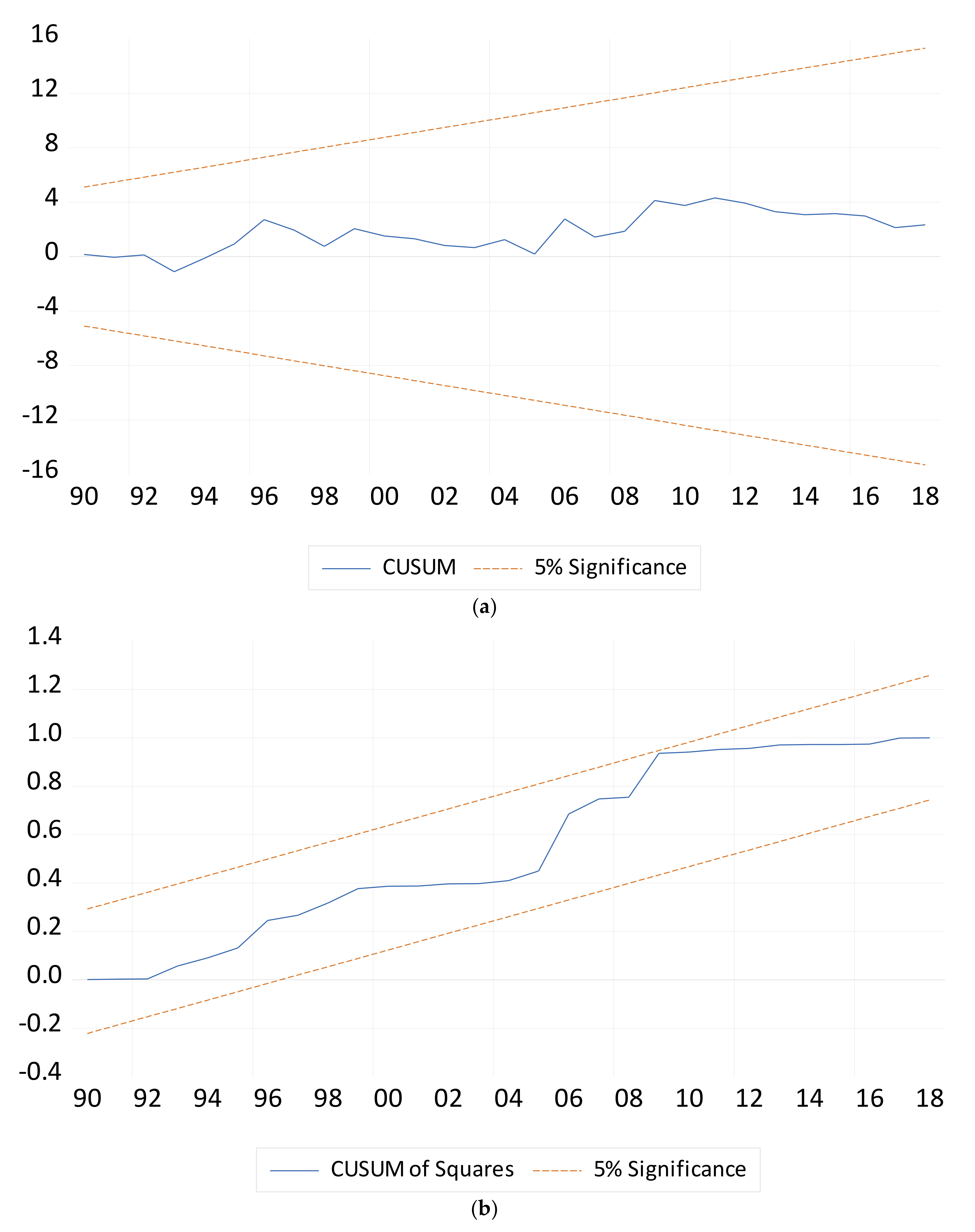
The number of tourist arrivals, economic growth, and primary energy in Australia has increased many times over the last five decades (Table 1). For example, the number of tourist arrivals during 2018 was 17 times greater than that in 1976, and GDP per capita doubled during the same period. Furthermore, per capita energy consumption surged by 25%. Although this study’s primary variable of interest was the number of tourist arrivals, this study also included other key control variables that affect energy consumption levels based on the existing literature. The study investigated whether tourist arrivals have a long-run cointegrating relationship with per capita energy consumption. Furthermore, this study conducted several diagnostic tests to estimate the model’s validity, along with the cointegration test. Subsequently, this study also employed FMOLS and DOLS regression further to analyse the relationship between the variables of interest. According to the diagnostic tests, the time-series data (log form of variables) did not have heteroscedasticity or serial correlation problems. The residual of the model was normally distributed, and the model passed the stability test. The ADF and PP unit root tests indicated that the variables had unit roots at the level and were stationary on their first difference. As reported in Table 4, the null hypothesis of no unit root could not be rejected at levels for all variables in the ADF test using both trend and no trend intercept options.

This study conducted multivariate cointegration tests. The multivariate cointegration test included a log of energy consumption as the dependent variable and all other variables as the explanatory variables. Given that the estimated variables of this study had a common stochastic trend (stationary at the same level), it was possible that they were cointegrated [87]. The multivariate cointegration test demonstrated at least one cointegrating relationship among the variables using the JJ test. To further explore the long-run association, ARDL bound tests, and BH cointegration tests were employed. The results indicated that tourist arrivals have a long-run cointegrating relationship with per capita energy consumption in Australia. Several past studies conducted with data from other comparable countries concluded that an increasing number of tourist arrivals leads to higher energy consumption or CO₂ emissions [5,43,52,87].

Using the ARDL technique, this study further established long-run and short-run dynamics between tourist arrivals and energy consumption. The signs of the coefficients were adherent to the economic model. Hence, this study concluded that international tourism has a positive and statistically significant effect on energy consumption. This is understandable because increased tourist arrivals increase economic activities and production (both goods and services), leading to higher energy consumption. For example, Tang et al. [52] commented that tourism-related infrastructures, facilities and activities necessitate additional energy, such as oil and electricity, for smooth operations, and Liu et al. [88] and Nepal et al. [43] also stated that tourism-related transportation is a significant contributor to energy consumption. Therefore, an increase in tourist arrivals increases energy demand. However, tourism in remote areas for instance, for hiking or for exploring the forest, may not require as much energy for electricity as required for tourism in the built environment. For example, tourism in the UAE may result in more energy consumption than the same tourist visiting the Mount Kilimanjaro. This also implies that weather along with the type of tourism attraction impacts energy consumption in a varied level. Other variables GDP per capita, CAP, and FD positively correlated with increased production; hence, it was reasonable to deduce a long-run cointegration with energy consumption [89]. Identical findings are available from studies from other comparable economies [90,91,92]. Growth in output (i.e., GDP) requires higher energy consumption, leading to environmental pollution [93], and FD develops new industries and production lines while also impacting emission and pollution.

After establishing the long-run association and ensuring the stability of the model, FMOLS and DOLS tests were performed. The results indicated a positive and significant relationship between international tourist arrivals and energy consumption in Australia. Noticeably, no existing studies used Australian data; therefore, this is among the preliminary studies to conclude that tourism affects energy consumption in Australia. In the pre-COVID years, the number of tourist arrivals was around one third of the total population of Australia. The increases both in energy consumption and population were roughly aligned. Past literature has commented that population growth increases urbanization, which increases the demand for energy consumption [63]. However, this research shows that the population does not affect primary energy consumption per capita in either the long or short run. This result aligns withLiu et al. [94], who has found that the negative elasticity of population to energy consumption in China was 0.211. Their results revealed that a 1% rise in population would decline energy use by 0.211% on a national scale. Similarly, the authors found that population density decreased energy use by 0.239% in the central, 0.218% in the western and 0.065% in the eastern regions of China. Azam et al. [95] found that population growth had a negative coefficient, implying decreased energy consumption in Thailand and Indonesia. The negative coefficient for the total population is logical because, if the total population increases, all other things being constant, per capita energy consumption would reduce. This result is consistent with previous findings conducted in China and Indonesia [94,95] as the total population would decrease the average energy demand.

No significant long-run relationship was observed between gross fixed capital formations and energy consumption. It is to note that Australia’s industry structure, energy consumption and nature of FD are significantly different from other developed nations. The estimated causal relationships of this study are authentic only in terms of Australia. Hence, generalization of the study results requires some cautions. According to our knowledge, no studies have yet examined the long-run relationship between total population, FD and energy consumption for Australia with time-series data.

7. Conclusions and Policy Implications

This study examined the effect of tourist arrivals on energy consumption by controlling GDP, capital, total population and financial development. This study used data from 1976 to 2018 in Australia. Three cointegrating techniques—ARDL bound, JJ and BH tests—were employed to confirm the long-run relationship between the variables. This study’s findings demonstrated a long-run cointegrating relationship between international tourist arrivals and energy consumption in Australia. Moreover, the results revealed that GDP, gross fixed capital formation and financial development contributed to Australia’s rising energy consumption.

The outcomes of this research have several policy implications. Given that rising energy consumption is significantly associated with climate change and carbon emissions, appropriate policies are required to reduce tourism-induced energy consumption in Australia. One of the potential requirements could be that policymakers provide an incentive to the tourism industry’s key stakeholders to adopt cleaner energies, carbon-neutral transportation and hybrid energies to achieve the desired level of carbon emission reductions. Hotels and other similar facilities could be encouraged to generate power from renewable sources. The government could provide tax rebates or low-cost (e.g., interest-free) financing opportunities for purchasing and installing environment-friendly technologies. Further studies may be conducted to examine the effectiveness of policies aiming at switching to renewable energy sources for Australia’s tourism industry and the cost-effectiveness of establishing green-energy-designed tourism in Australia to minimize the use of energy. Furthermore, researchers are urged to test the robustness of the conclusions using multiple econometric models on the same sample data. Further research is needed for policy makers, government authorities and tourism relalated officials to examine the impact of tourism and energy relationship in the context of current COVID-19 situation using air transport, travel and tourism sector. This review of disruption by COVID would help to cope with the economy and can be expanded to heal the economic crisis.

This study has filled up an important research gap by examining the linkage between tourism and energy consumption in the case of Australia because this is the first ever study in Australia context as per the author’s knowledge. Our main contribution is that we have found significant effect of tourist arrivals on energy consumption that has potential detrimental effects on the environment which policy makers should consider seriously in formulating and executing energy- and tourism-related policies. Our findings have implications not only for Australia but also for other countries.

References

1. WTTC Economic Impact Reports. Available online: https://wttc.org/Research/Economic-Impact (accessed on 3 January 2021).
2. Kyara, V.C.; Rahman, M.M.; Khanam, R. Tourism expansion and economic growth in Tanzania: A causality analysis. Heliyon 2021, 7, e06966. [Google Scholar] [CrossRef] [PubMed]
3. Antara, M.; Sumarniasih, M.S. Role of Tourism in Economy of Bali and Indonesia. J. Tour. Hosp. Manag. 2017, 5, 34–44. [Google Scholar] [CrossRef] [Green Version]
4. Dogru, T.; Bulut, U. Is Tourism an Engine for Economic Recovery? Theory and Empirical Evidence. Tour. Manag. 2018, 67, 425–434. [Google Scholar] [CrossRef]
5. Dogan, E.; Aslan, A. Exploring the Relationship Among CO2 Emissions, Real GDP, Energy Consumption and Tourism in the EU and Candidate Countries: Evidence from Panel Models Robust to Heterogeneity and Cross-Sectional Dependence. Renew. Sustain. Energy Rev. 2017, 77, 239–245. [Google Scholar] [CrossRef]
6. Koçak, E.; Ulucak, R.; Ulucak, Z.Ş. The impact of tourism developments on CO2 emissions: An advanced panel data estimation. Tour. Manag. Perspect. 2020, 33, 100611. [Google Scholar] [CrossRef]
7. Nepal, S.K. Tourism-Induced Rural Energy Consumption in the Annapurna Region of Nepal. Tour. Manag. 2008, 29, 89–100. [Google Scholar] [CrossRef]
8. Ișik, C.; Ahmad, M.; Pata, U.K.; Ongan, S.; Radulescu, M.; Adedoyin, F.F.; Bayraktaroğlu, E.; Aydın, S.; Ongan, A. An evaluation of the tourism-induced environmental Kuznets curve (T-EKC) hypothesis: Evidence from G7 Countries. Sustainability 2020, 12, 9150. [Google Scholar]
9. Dogru, T.; Bulut, U.; Kocak, E.; Isik, C.; Suess, C.; Sirakaya-Turk, E. The nexus between tourism, economic growth, renewable energy consumption, and carbon dioxide emissions: Contemporary evidence from OECD countries. Environ. Sci. Pollut. Res. 2020, 27, 40930–40948. [Google Scholar] [CrossRef]
10. Işik, C.; Doğan, E.; Ongan, S. Analyzing the tourism–energy–growth nexus for the top 10 most-visited countries. Economies 2017, 5, 40. [Google Scholar] [CrossRef] [Green Version]
11. Rahman, S.M.; Miah, M.D. The impact of sources of energy production on globalization: Evidence from panel data analysis. Renew. Sustain. Energy Rev. 2017, 74, 110–115. [Google Scholar] [CrossRef]
12. Li, S.; Zhang, J.; Ma, Y. Financial development, environmental quality and economic growth. Sustainability 2015, 7, 9395–9416. [Google Scholar] [CrossRef] [Green Version]
13. Shahbaz, M.; Mallick, H.; Mahalik, M.K.; Loganathan, N. Does globalization impede environmental quality in India? Ecol. Indic. 2015, 52, 379–393. [Google Scholar] [CrossRef] [Green Version]
14. Dogru, T.; Isik, C.; Sirakaya-Turk, E. The balance of trade and exchange rates: Theory and contemporary evidence from tourism. Tour. Manag. 2019, 74, 12–23. [Google Scholar] [CrossRef]
15. Işık, C.; Sirakaya-Turk, E.; Ongan, S. Testing the efficacy of the economic policy uncertainty index on tourism demand in USMCA: Theory and evidence. Tour. Econ. 2020, 26, 1344–1357. [Google Scholar] [CrossRef]
16. Pan, Y.; Weng, G.; Li, C.; Li, J. Coupling coordination and influencing factors among tourism carbon emission, tourism economic and tourism innovation. Int. J. Environ. Res. Public Health 2021, 18, 1601. [Google Scholar] [CrossRef]
17. Wilson, S.; Fesenmaier, D.R.; Fesenmaier, J.; Van Es, J.C. Factors for success in rural tourism development. J. Travel Res. 2001, 40, 132–138. [Google Scholar] [CrossRef]
18. Luo, J.M.; Fan, Y.; Shang, Z. Analysis of Critical Success Factors for Entertainment Tourism Destinations: The Supply Perspective. J. Qual. Assur. Hosp. Tour. 2021, 22, 1–24. [Google Scholar]
19. Gia, B.H. Some Solutions for Sustainable Agricultural Tourism Development in the Mekong Delta in Vietnam; E3S Web of Conferences, 2021; EDP Sciences: Les Ulis, France, 2021; p. 00063. [Google Scholar]
20. Cham, T.-H.; Lim, Y.-M.; Sia, B.-C.; Cheah, J.-H.; Ting, H. Medical tourism destination image and its relationship with the intention to revisit: A study of Chinese medical tourists in Malaysia. J. China Tour. Res. 2021, 17, 163–191. [Google Scholar] [CrossRef]
21. Pastén, R.; Saens, R.; Contreras Marin, R. Does Energy Use cause Economic Growth in Latin America? Appl. Econ. Lett. 2015, 22, 1399–1403. [Google Scholar] [CrossRef]
22. Khanal, A. Does Energy Consumption impact the Environment? Evidence from Australia using the JJ Bayer-Hanck Cointegration Technique and the Autoregressive Distributed Lag Test. Int. J. Energy Econ. Policy 2021, 11, 185–194. [Google Scholar] [CrossRef]
23. Moutinho, V.; Costa, C.; Bento, J.P.C. The impact of energy efficiency and economic productivity on CO2 emission intensity in Portuguese tourism industries. Tour. Manag. Perspect. 2015, 16, 217–227. [Google Scholar] [CrossRef]
24. Akhmat, G.; Zaman, K.; Shukui, T.; Sajjad, F. Does Energy Consumption Contribute to Climate Change? Evidence from major Regions of the World. Renew. Sustain. Energy Rev. 2014, 36, 123–134. [Google Scholar] [CrossRef]
25. Shi, Y.; Yu, M. Assessing the Environmental Impact and cost of the Tourism-Induced CO2, NOX, SOX emission in China. Sustainability 2021, 13, 604. [Google Scholar] [CrossRef]
26. William, J. Drivers: Economic Activity as a driver of Environmental Change in: Australia State of the Environment 2016. Available online: https://soe.environment.gov.au/theme/drivers/topic/economic-activity-driver-environmental-change (accessed on 19 June 2021).
27. Judd, B.; Tonkin, L. Vale the Great Australian Summer. Available online: https://www.abc.net.au/news/2020-02-29/australian-summer-season-lost-to-bushfires-floods-and-drought/11994310 (accessed on 17 May 2021).
28. Roman, M.; Niedziółka, A.; Krasnodębski, A. respondents’ involvement in tourist activities at the Time of the COVID-19 Pandemic. Sustainability 2020, 12, 9610. [Google Scholar] [CrossRef]
29. Williams, N.L.; Wassler, P.; Ferdinand, N. Tourism and the COVID-(mis) infodemic. J. Travel Res. 2020. [Google Scholar] [CrossRef]
30. Riley, R.W.; Van Doren, C.S. Movies as Tourism Promotion: A ‘Pull’factor in a ‘Push’location. Tour. Manag. 1992, 13, 267–274. [Google Scholar] [CrossRef]
31. Breakey, N.; Ding, P.; Lee, T. Impact of Chinese outbound tourism to Australia: Reviewing the past; implications for the future. Curr. Issues Tour. 2008, 11, 587–603. [Google Scholar] [CrossRef]
32. Reisinger, Y.; Turner, L. Cross-Cultural differences in Tourism: Indonesian Tourists in Australia. Tour. Manag. 1997, 18, 139–147. [Google Scholar] [CrossRef]
33. Kellogg, R.; Wolff, H. Daylight Time and Energy: Evidence from an Australian Experiment. J. Environ. Econ. Manag. 2008, 56, 207–220. [Google Scholar] [CrossRef]
34. Ryan, P.; Pavia, M. Australian Residential Energy End-Use—Trends and Projections to 2030. In Proceedings of the 2016 ACEEE Summer Study on Energy Efficiency in Buildings, Pacific Grove, CA, USA, 21–26 August 2016. [Google Scholar]
35. Lütkepohl, H.; Krätzig, M.; Phillips, P.C. Applied Time Series Econometrics; Cambridge University Press: Cambridge, UK, 2004. [Google Scholar]
36. Ali, W.; Sadiq, F.; Kumail, T.; Li, H.; Zahid, M.; Sohag, K. A Cointegration Analysis of Structural Change, International Tourism and Energy Consumption On CO2 Emission In Pakistan. Curr. Issues Tour. 2020, 23, 3001–3015. [Google Scholar] [CrossRef]
37. Ben Jebli, M.; Hadhri, W. The Dynamic Causal links Between CO2 Emissions from Transport, Real GDP, Energy Use and International Tourism. Int. J. Sustain. Dev. World Ecol. 2018, 25, 568–577. [Google Scholar] [CrossRef]
38. Gokmenoglu, K.; Taspinar, N. The Relationship Between CO2 Emissions, Energy Consumption, Economic Growth and FDI: The Case of Turkey. J. Int. Trade Econ. Dev. 2016, 25, 706–723. [Google Scholar] [CrossRef]
39. Katircioglu, S.T.; Feridun, M.; Kilinc, C. Estimating Tourism-Induced Energy Consumption and CO2 Emissions: The Case of Cyprus. Renew. Sustain. Energy Rev. 2014, 29, 634–640. [Google Scholar] [CrossRef]
40. Katircioglu, S.T. International Tourism, Energy Consumption, and Environmental Pollution: The Case of Turkey. Renew. Sustain. Energy Rev. 2014, 36, 180–187. [Google Scholar] [CrossRef]
41. Liu, Y.; Kumail, T.; Ali, W.; Sadiq, F. The Dynamic Relationship between CO2 Emission, International Tourism and Energy Consumption in Pakistan: A Cointegration Approach. Tour. Rev. 2019, 74, 761–779. [Google Scholar] [CrossRef]
42. Naradda Gamage, S.K.; Hewa Kuruppuge, R.; Haq, I.U. Energy Consumption, Tourism Development, and Environmental Degradation in Sri Lanka. Energy Sources Part B Econ. Plan. Policy 2017, 12, 910–916. [Google Scholar] [CrossRef]
43. Nepal, R.; al Irsyad, M.I.; Nepal, S.K. Tourist Arrivals, Energy Consumption and Pollutant Emissions In a Developing Economy–Implications for Sustainable Tourism. Tour. Manag. 2019, 72, 145–154. [Google Scholar] [CrossRef]
44. Selvanathan, E.A.; Jayasinghe, M.; Selvanathan, S. Dynamic Modelling of Inter-Relationship Between Tourism, Energy Consumption, CO2 Emissions and Economic Growth in South Asia. Int. J. Tour. Res. 2020, 23, 597–610. [Google Scholar] [CrossRef]
45. Sghaier, A.; Guizani, A.; Jabeur, S.B.; Nurunnabi, M. Tourism Development, Energy Consumption and Environmental Quality in Tunisia, Egypt and Morocco: A Trivariate Analysis. GeoJournal 2019, 84, 593–609. [Google Scholar] [CrossRef]
46. Zhang, L.; Gao, J. Exploring the Effects of International Tourism on China’s Economic Growth, Energy Consumption and Environmental Pollution: Evidence from a Regional Panel Analysis. Renew. Sustain. Energy Rev. 2016, 53, 225–234. [Google Scholar] [CrossRef]
47. Amin, S.B.; Kabir, F.A.; Khan, F. Tourism and Energy Nexus in Selected South Asian Countries: A Panel Study. Curr. Issues Tour. 2020, 23, 1963–1967. [Google Scholar] [CrossRef]
48. Isik, C.; Dogru, T.; Turk, E.S. A Nexus of Linear and Non-Linear Relationships between Tourism Demand, Renewable Energy Consumption, and Economic Growth: Theory and Evidence. Int. J. Tour. Res. 2018, 20, 38–49. [Google Scholar] [CrossRef]
49. Gokmenoglu, K.K.; Eren, B.M. The role of international tourism on energy consumption: Empirical evidence from Turkey. Curr. Issues Tour. 2020, 23, 1059–1065. [Google Scholar] [CrossRef]
50. Solarin, S.A. Tourist Arrivals and Macroeconomic Determinants of CO2 Emissions in Malaysia. Anatolia 2014, 25, 228–241. [Google Scholar] [CrossRef]
51. Alola, A.A.; Alola, U.V. Agricultural Land Usage and Tourism Impact on Renewable Energy Consumption Among Coastline Mediterranean Countries. Energy Environ. 2018, 29, 1438–1454. [Google Scholar] [CrossRef]
52. Tang, C.F.; Tiwari, A.K.; Shahbaz, M. Dynamic Inter-Relationships among Tourism, Economic Growth and Energy Consumption in India. Geosystem Eng. 2016, 19, 158–169. [Google Scholar] [CrossRef]
53. Ali, Q.; Khan, M.T.I.; Khan, M.N.I. Dynamics between Financial Development, Tourism, Sanitation, Renewable Energy, Trade and Total Reserves in 19 Asia Cooperation Dialogue Members. J. Clean. Prod. 2018, 179, 114–131. [Google Scholar] [CrossRef]
54. Shi, H.; Li, X.; Zhang, H.; Liu, X.; Li, T.; Zhong, Z. Global Difference in the Relationships Between Tourism, Economic Growth, CO2 Emissions, And Primary Energy Consumption. Curr. Issues Tour. 2020, 23, 1122–1137. [Google Scholar] [CrossRef]
55. Gozgor, G.; Lau, C.K.M.; Lu, Z. Energy Consumption and Economic Growth: New Evidence from the OECD Countries. Energy 2018, 153, 27–34. [Google Scholar] [CrossRef] [Green Version]
56. Rahman, M.M.; Alam, K. Exploring the driving factors of economic growth in the world’s largest economies. Heliyon 2021, 7, e07109. [Google Scholar] [CrossRef]
57. Rahman, M.M. The dynamic nexus of energy consumption, international trade and economic growth in BRICS and ASEAN countries: A panel causality test. Energy 2021, 229, 120679. [Google Scholar] [CrossRef]
58. Rahman, M.M.; Rana, R.H.; Barua, S. The drivers of economic growth in South Asia: Evidence from a dynamic system GMM approach. J. Econ. Stud. 2019, 46, 564–577. [Google Scholar] [CrossRef]
59. Saidi, K.; Rahman, M.M.; Amamri, M. The causal nexus between economic growth and energy consumption: New evidence from global panel of 53 countries. Sustain. Cities Soc. 2017, 33, 45–56. [Google Scholar] [CrossRef]
60. Topcu, E.; Altinoz, B.; Aslan, A. Global Evidence from the link between Economic Growth, Natural Resources, Energy Consumption, and Gross Capital Formation. Resour. Policy 2020, 66, 101622. [Google Scholar] [CrossRef]
61. Chiu, Y.-B.; Lee, C.-C. Effects of Financial Development on Energy Consumption: The Role of Country Risks. Energy Econ. 2020, 90, 104833. [Google Scholar] [CrossRef]
62. Saud, S.; Baloch, M.A.; Lodhi, R.N. The Nexus Between Energy Consumption and Financial Development: Estimating the Role of Globalization in Next-11 Countries. Environ. Sci. Pollut. Res. 2018, 25, 18651–18661. [Google Scholar]
63. Shahbaz, M.; Lean, H.H. Does Financial Development increase Energy Consumption? The Role of Industrialization and Urbanization in Tunisia. Energy Policy 2012, 40, 473–479. [Google Scholar] [CrossRef] [Green Version]
64. ABS Overseas Arrivals And Departures (Cat. No. 3401.0), Canberra, Australia. Available online: https://www.abs.gov.au/Ausstats/[email protected]/glossary/3401.0 (accessed on 22 February 2021).
65. World Bank World Development Indicator. Available online: https://datacatalog.worldbank.org/dataset/world-development-indicators (accessed on 22 March 2021).
66. BP Statistical Review Statistical Review of World Energy. Available online: https://www.bp.com/en/global/corporate/energy-economics/statistical-review-of-world-energy.html (accessed on 19 December 2020).
67. Omri, A.; Kahouli, B. Causal Relationships Between Energy Consumption, Foreign Direct Investment and Economic Growth: Fresh Evidence from Dynamic Simultaneous-Equations Models. Energy Policy 2014, 67, 913–922. [Google Scholar] [CrossRef] [Green Version]
68. Lütkepohl, H.; Xu, F. The role of the log transformation in forecasting economic variables. Empir. Econ. 2012, 42, 619–638. [Google Scholar] [CrossRef] [Green Version]
69. Dickey, D.A.; Fuller, W.A. Distribution of the Estimators for Autoregressive Time Series with a Unit Root. J. Am. Stat. Assoc. 1979, 74, 427–431. [Google Scholar]
70. Dickey, D.A.; Fuller, W.A. Likelihood Ratio Statistics for Autoregressive Time Series with a Unit Root. Econom. J. Econom. Soc. 1981, 49, 1057–1072. [Google Scholar] [CrossRef]
71. Phillips, P.C.; Perron, P. Testing for a unit root in time series regression. Biometrika 1988, 75, 335–346. [Google Scholar] [CrossRef]
72. Baker, D.; Merkert, R.; Kamruzzaman, M. Regional Aviation and Economic Growth: Cointegration and Causality Analysis In Australia. J. Transp. Geogr. 2015, 43, 140–150. [Google Scholar] [CrossRef]
73. Hamilton, J.D. Time Series Analysis; Princeton University Press: Princeton, NJ, USA, 2020. [Google Scholar]
74. Pesaran, M.H.; Shin, Y.; Smith, R.J. Bounds testing approaches to the analysis of level relationships. J. Appl. Econom. 2001, 16, 289–326. [Google Scholar] [CrossRef]
75. Johansen, S.; Juselius, K. Maximum Likelihood Estimation and Inference on Cointegration—With Appucations to the Demand for Money. Oxf. Bull. Econ. Stat. 1990, 52, 169–210. [Google Scholar] [CrossRef]
76. Bayer, C.; Hanck, C. Combining non-cointegration tests. J. Time Ser. Anal. 2013, 34, 83–95. [Google Scholar] [CrossRef]
77. Engle, R.F.; Granger, C.W. Co-Integration and Error Correction: Representation, Estimation, and Testing. Econom. J. Econom. Soc. 1987, 55, 251–276. [Google Scholar] [CrossRef]
78. Johansen, S. Estimation and Hypothesis testing of Cointegration Vectors in Gaussian Vector Autoregressive Models. Econom. J. Econom. Soc. 1991, 59, 1551–1580. [Google Scholar] [CrossRef]
79. Banerjee, A.; Dolado, J.; Mestre, R. Error-correction mechanism tests for cointegration in a single-equation framework. J. Time Ser. Anal. 1998, 19, 267–283. [Google Scholar] [CrossRef] [Green Version]
80. Boswijk, H.P. Efficient inference on cointegration parameters in structural error correction models. J. Econom. 1995, 69, 133–158. [Google Scholar] [CrossRef] [Green Version]
81. Etokakpan, M.U.; Solarin, S.A.; Yorucu, V.; Bekun, F.V.; Sarkodie, S.A. Modeling natural gas consumption, capital formation, globalization, CO2 emissions and economic growth nexus in Malaysia: Fresh evidence from combined cointegration and causality analysis. Energy Strategy Rev. 2020, 31, 100526. [Google Scholar] [CrossRef]
82. Baloch, M.A.; Suad, S. Modeling the Impact of Transport Energy Consumption on CO2 Emission in Pakistan: Evidence from ARDL Approach. Environ. Sci. Pollut. Res. 2018, 25, 9461–9473. [Google Scholar]
83. Ali, S.; Ying, L.; Anjum, R.; Nazir, A.; Shalmani, A.; Shah, T.; Shah, F. Analysis on the Nexus of CO2 Emissions, Energy Use, Net Domestic Credit, and GDP in Pakistan: An ARDL Bound Testing Analysis. Environ. Sci. Pollut. Res. 2021, 28, 4594–4614. [Google Scholar] [CrossRef]
84. Rahman, M.M.; Kashem, M.A. Carbon Emissions, Energy Consumption and Industrial Growth in Bangladesh: Empirical Evidence from ARDL Cointegration and Granger Causality Analysis. Energy Policy 2017, 110, 600–608. [Google Scholar] [CrossRef]
85. Shahbaz, M.; Farhani, S.; Ozturk, I. Do coal consumption and industrial development increase environmental degradation in China and India? Environ. Sci. Pollut. Res. 2015, 22, 3895–3907. [Google Scholar] [CrossRef] [PubMed]
86. Brown, R.L.; Durbin, J.; Evans, J.M. Techniques for testing the constancy of regression relationships over time. J. R. Stat. Soc. Ser. B Methodol. 1975, 37, 149–163. [Google Scholar] [CrossRef]
87. Tiwari, A.K.; Ozturk, I.; Aruna, M. Tourism, Energy Consumption and Climate Change in OECD Countries. Int. J. Energy Econ. Policy 2013, 3, 247–261. [Google Scholar]
88. Liu, J.; Feng, T.; Yang, X. The Energy Requirements and Carbon Dioxide Emissions of Tourism Industry of Western China: A Case of Chengdu City. Renew. Sustain. Energy Rev. 2011, 15, 2887–2894. [Google Scholar] [CrossRef]
89. Rahman, M.M.; Velayutham, E. Renewable and non-renewable energy consumption-economic growth nexus: New evidence from South Asia. Renew. Energy 2020, 147, 399–408. [Google Scholar] [CrossRef]
90. Khan, I.; Hou, F.; Le, H.P. The Impact of Natural Resources, Energy Consumption, and Population Growth on Environmental Quality: Fresh Evidence from the United States of America. Sci. Total Environ. 2020, 754, 142222. [Google Scholar] [CrossRef]
91. Mahadevan, R.; Asafu-Adjaye, J. Energy Consumption, Economic Growth and Prices: A Reassessment Using Panel VECM for Developed and Developing Countries. Energy Policy 2007, 35, 2481–2490. [Google Scholar] [CrossRef]
92. Soytas, U.; Sari, R. Energy Consumption, Economic Growth, and Carbon Emissions: Challenges faced by An EU Candidate Member. Ecol. Econ. 2009, 68, 1667–1675. [Google Scholar] [CrossRef]
93. Khanal, A. The role of ICT and Energy Consumption on Carbon Emissions: An Australian Evidence using Cointegration test and ARDL Long-run and Short-run Methodology. Int. J. Energy Econ. Policy 2021, 11, 441–449. [Google Scholar] [CrossRef]
94. Liu, Y.; Zhou, Y.; Wu, W. Assessing the impact of Population, Income and Technology on Energy Consumption and Industrial Pollutant Emissions in China. Appl. Energy 2015, 155, 904–917. [Google Scholar] [CrossRef]
95. Azam, M.; Khan, A.Q.; Zaman, K.; Ahmad, M. Factors determining energy consumption: Evidence from Indonesia, Malaysia and Thailand. Renew. Sustain. Energy Rev. 2015, 42, 1123–1131. [Google Scholar] [CrossRef]
Figure 1. Trend lines for variables of interest.
Sustainability 13 10800 g001
Figure 2. (a) Plot of CUSUM of recursive residuals. (b) Plot of cumulative sum of recursive squares (CUSUMSQ).
Sustainability 13 10800 g002