Ultra Short-Term Wind Power Forecasting Based on Sparrow Search Algorithm Optimization Deep Extreme Learning Machine

Abstract

Improving the accuracy of wind power forecasting is an important measure to deal with the uncertainty and volatility of wind power. Wind speed and wind direction are the most important factors affecting the power generation of wind turbines. In this paper, we propose a wind power forecasting method that combines the sparrow search algorithm (SSA) with the deep extreme learning machine (DELM). Based on the DELM model, the length of the time series’ influence on the performance of the neural network is validated through the comparison of the forecast error indexes, and the optimal time series length of the wind power is determined. The sparrow search algorithm is used to optimize its parameters to solve the problem of random changes in model input weights and thresholds. The proposed SSA-DELM model is validated using the measured data of a certain wind turbine, and various forecasting indexes are compared with several current wind power forecasting methods. The experimental results show that the proposed model has better performance in ultra-short-term wind power forecasting, and its coefficient of determination (R²), mean absolute error (MAE), and root mean square error (RMSE) are 0.927, 69.803, and 115.446, respectively.

1. Introduction

At present, countries all over the world are paying more attention to the development and use of renewable energy such as wind energy, solar energy, and geothermal energy [1]. Among all kinds of renewable energy, wind power transmission, distribution technology, and wind power grid-connected technology are becoming more and more mature. Vigorously developing wind power technology has become the consensus of most countries in the world [2]. In recent years, wind power has developed rapidly in China. By the end of 2020 and 2050, the total installed capacity of wind power in China will exceed 200 and 1000 GW, respectively [3]. According to data released by the International Renewable Energy Agency, more than 80% of all new power generation capacity in 2020 will be renewable energy, of which solar and wind energy account for 91%. From 2021 to 2030, the global wind power industry is expected to add 1TW of installed capacity [4]. However, the inherent randomness and volatility of wind energy have brought severe challenges to the power grid, and a large number of grid-connected wind power have caused more and more difficulties for the grid dispatching center. The balance cost of the power grid is gradually increasing, and the accurate prediction of wind power has important engineering significance for solving the above problems [5,6,7].

The ultra-short-term wind power prediction aims to predict the wind power data within 4 h, which can provide an important reference for the real-time dispatch of the power system [8]. Ultra-short-term wind power prediction methods can be divided into two categories: physical methods and statistical methods [9]. The calculation process of physical methods is complicated, and the technical threshold is high. Not all participants can obtain the necessary physical information [10]. Compared with physical methods, statistical methods have attracted much attention in recent years. This method establishes the connection among historical wind power data, numerical weather prediction (NWP) data, historical data, and real-time data through one or more algorithms and then realizes the prediction of the output power of the wind farm. This method is easy to model and has strong adaptability to sample learning. It has been widely used in the wind power industry and other projects that require prediction [11]. An et al. used the particle swarm optimization algorithm (PSO) to optimize the extreme learning machine (ELM) and combined them with the Adaboost integrated learning model to make a short-term prediction of wind power [12]. However, the model takes wind speed and direction as input and wind power as output. The predictive performance of the model is very dependent on the accuracy of the NWP. The training time required is rather long. In [13], Li et al. use support vector machines to predict the wind turbine data of the La Haute Borne wind farm in autumn, and the absolute error of all sample points can be less than 25%. In [14], the researchers use the method of least square support vector machine (LSSVM) to effectively predict the deterministic trend, periodic term, and random component of the next 168 h and then obtain the wind power forecast value. However, the ability of the above methods to extract the deep features of wind power data is slightly insufficient, and the generalization ability is not suitable when dealing with more complex regression tasks [15]. Deep learning methods can fully mine data information, and a deep extreme learning machine (DELM) is one of the most representative methods [16]. When facing high-dimensional data, DELM can directly use it as the input of the network for training and has suitable generalization performance. DELM has better prediction performance than traditional neural network methods such as generalized regression neural network (GRNN) and probabilistic neural network (PNN) and has been widely used in medical, military, wireless sensor networks, and other fields [17,18,19,20,21].

In the process of DELM training, the input layer weight and threshold are randomly generated orthogonal random matrices, which greatly affect the prediction effect of DELM. Therefore, it is very necessary to use a method to optimize the selection of the above parameters to effectively improve the prediction accuracy of the model. In recent years, many scholars around the world have begun to study the combination of optimization algorithms and prediction models to achieve optimization of prediction model parameters [22]. Multiple algorithms such as genetic algorithm, whale optimization algorithm, differential evolution algorithm, cuckoo search algorithm, and sparrow search algorithm have been successfully used to optimize power prediction models [6,23,24,25,26]. In [27], M. H. Ahmadi et al. use genetic algorithms to optimize the hyperparameters embedded in the least-squares support vector machine model and use the size, concentration, and temperature of nanoparticles as input variables to predict the thermal conductivity of Al₂O₃/EG. Literature [28] uses genetic algorithms to calculate the optimal values of radial bias function’s spread and maximum neuron number (MNN), which can accurately predict the thermal resistance of the pulsating heat pipes (PHP) filled with ethanol. Literature [29] uses a group method of data handling (GMDH) neural network to predict the physical properties of PHPs with water as the working fluid, including thermal resistance and effective thermal conductivity. Literature [30] proposed a short-term wind power prediction method based on a whale algorithm optimization support vector machine. This model overcomes the shortcomings of support vector machines that are easy to fall into local minima and uses a whale algorithm to optimize the penalty coefficient and kernel parameters of SVM. The optimized SVM prediction performance is significantly improved, and the RMSE is reduced from 49.48 to 32.49, but the number of iterations required to achieve convergence is still relatively large. Literature [31] uses differential evolution algorithm to optimize the kernel extreme learning machine to achieve the purpose of predicting wind power, which makes the optimized kernel extreme learning machine (KELM) more accurate than the unoptimized KELM by 8.34%, but the differential evolution algorithm is prone to premature convergence, especially in the case of solving complex functions. Literature [32] uses the cuckoo search optimization algorithm (CSO) to optimize the parameters of the improved long-term, short-term memory network. The proposed model has fewer statistical performance errors for indexes such as MAE, mean absolute scale error (MASE), and RMSE. However, the lack of vitality of CSO makes it only suitable for continuous functions. It can be seen that the above three swarm intelligence algorithms can play an optimal effect and greatly reduce the prediction error, but the convergence speed needs to be improved, and the local optimum still needs to be avoided.

The sparrow search algorithm was proposed by Xue in 2020. The algorithm has the characteristics of fast convergence, high efficiency, simple algorithm, and large expansion space [33]. Literature [34] uses the sparrow search algorithm (SSA) to optimize the selection of the proton exchange membrane fuel cell stack model parameters, and the results show that the SSA algorithm is more superior to gray relational analysis (GRA). Literature [35] uses SSA to optimize convolutional neural network (CNN) to improve the efficiency of CNN in terms of consistency and accuracy. Literature [36] optimizes the parameter selection of support vector machine (SVM) through SSA, and the constructed SSA-SVM diagnosis model effectively improves the accuracy of wind turbine fault diagnosis. This article intends to use SSA to optimize the DELM input layer weight and threshold so as to improve the prediction performance of DELM. At the same time, ultra-short-term wind power prediction can be accomplished only with accurate historical wind power data based on the proposed prediction model.

The main contributions of this work are presented as follows:

• The proposed SSA-ELM wind power prediction model is based on time series, and it’s less dependent on input data than models based on NWP data;
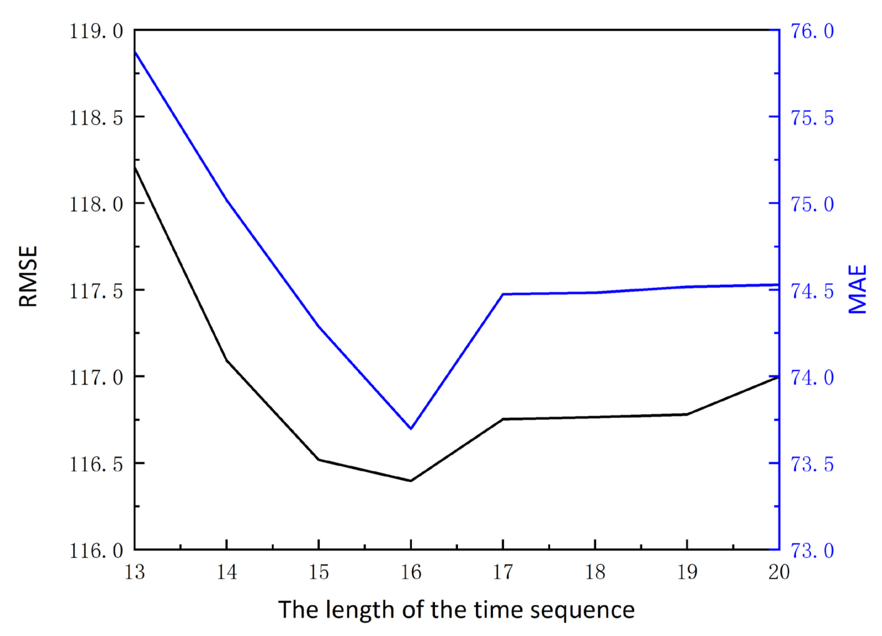
• The effect of the time series’ length on the prediction accuracy of the neural network model is verified. The method of optimizing the length of the time series is explained in detail;
• The sparrow search algorithm is combined with the deep extreme learning machine to forecast wind power for the first time. By dividing the sparrow population into three categories: discoverers, entrants, and guards, the input weights and thresholds of DELM are optimized. The prediction results are compared with several other optimized neural network models. The results show that the proposed model increases the speed of convergence and effectively avoids the optimization process from falling into the local optimum.

The rest of the paper is arranged as follows. In Section 2, the principles of extreme learning machine, deep extreme learning machine, and sparrow search algorithm are introduced in detail, and the SSA-DELM wind power prediction model is proposed. In Section 3, we first select an appropriate time sequence length and make a rolling forecast on the data. The results are compared with those of several current mainstream methods. Through the error analysis of multiple indicators, the validity and feasibility of the method proposed in this paper are verified. Finally, the conclusions are given in Section 4.

2. Materials and Methods

This section aims to briefly introduce the methods used in this study, including the deep extreme learning machine (DELM) method, sparrow search algorithm (SSA), and SSA-DELM model.

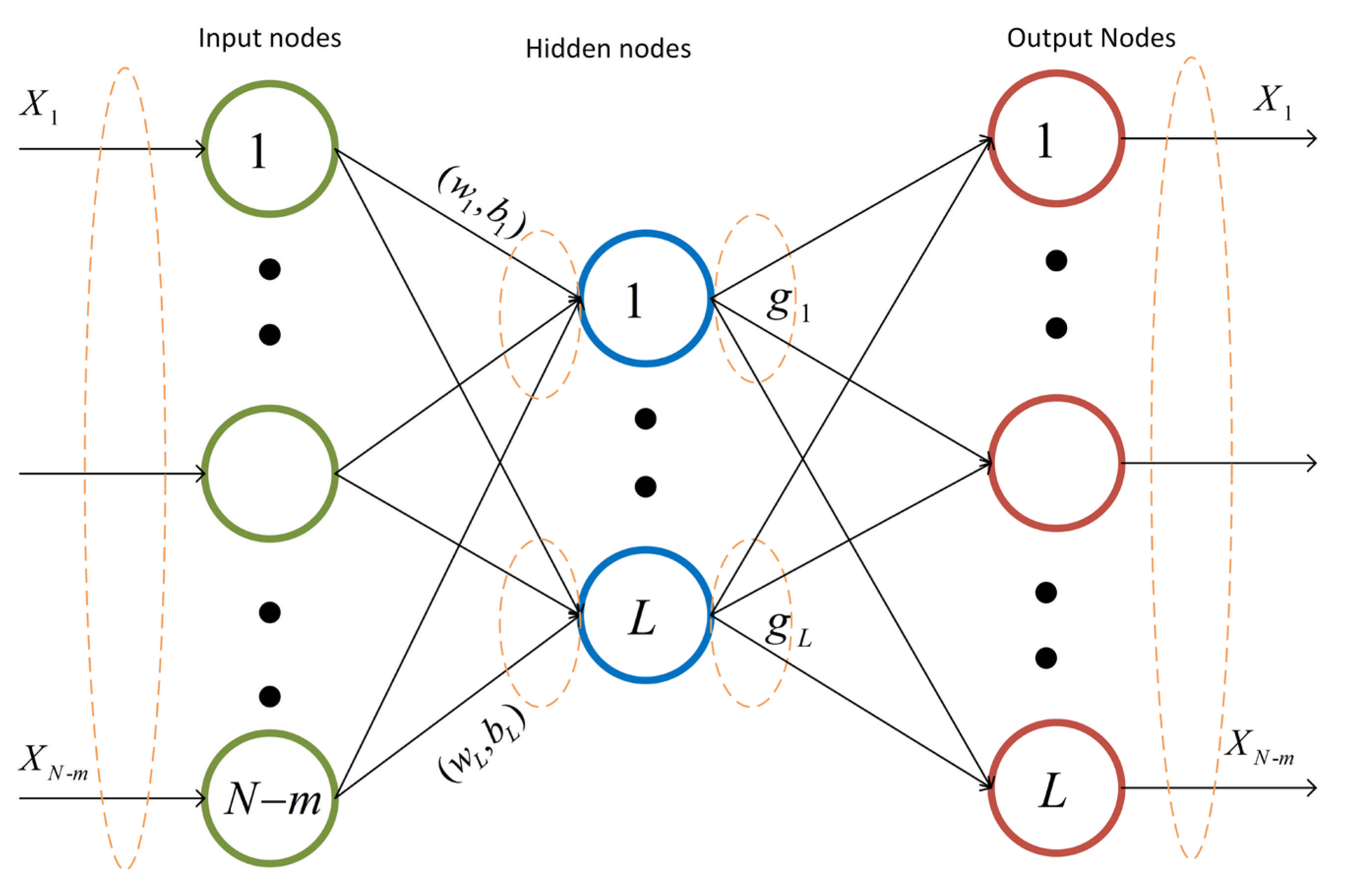
2.1. Extreme Learning Machine

The extreme learning machine (ELM) is a machine learning method based on a feedforward neural network [37]. Suppose there are currently N different wind power data $P_t$($t$= 1, 2, …, N). Continuous m wind power data are used to construct a one-dimensional vector $X_i={\left[P_i,P_{i+1,}\dots ,P_{i+m-1}\right]}^T$($i=1,2,\dots ,N-m)$, which serves as the input information for training samples. The input information of the (N − m) group of training samples can be obtained, where i represents the starting time of the training sample’s power data. The actual power data $P_{i+m}$ at the next moment of the vector $X_i$ is used as the expected predicted value, that is, the output of the ELM. The output is expressed as $Y_i=[P_{i+m}]$. The mathematical model of ELM is defined as follows:

$$Y_i={\displaystyle \sum _{j=1}^{L}g{\beta }_j\left(w_j·X_i+b_j\right)},i=1,2,\dots ,N-m$$

(1)

where $w_j$ is the input weight, ${\beta }_j$ is the output weight, $b_j$ is the threshold of the j-th hidden layer neuron, L is the number of hidden layer nodes, and g(x) is the activation function. ELM can optimize ${\beta }_j$ through neural network training to minimize the error of predicted value $Y_i$. The training process of ELM only needs one iteration, and the training time of the network is short. At the same time, the $w_j$ and $b_j$ of the ELM are randomly generated and do not need to be updated iteratively. Therefore, the ELM can solve the local minimum problem in the traditional neural network. However, the traditional ELM only contains one hidden layer, which makes it difficult for the accuracy of ultra-short-term wind power forecasting to achieve the expected purpose.

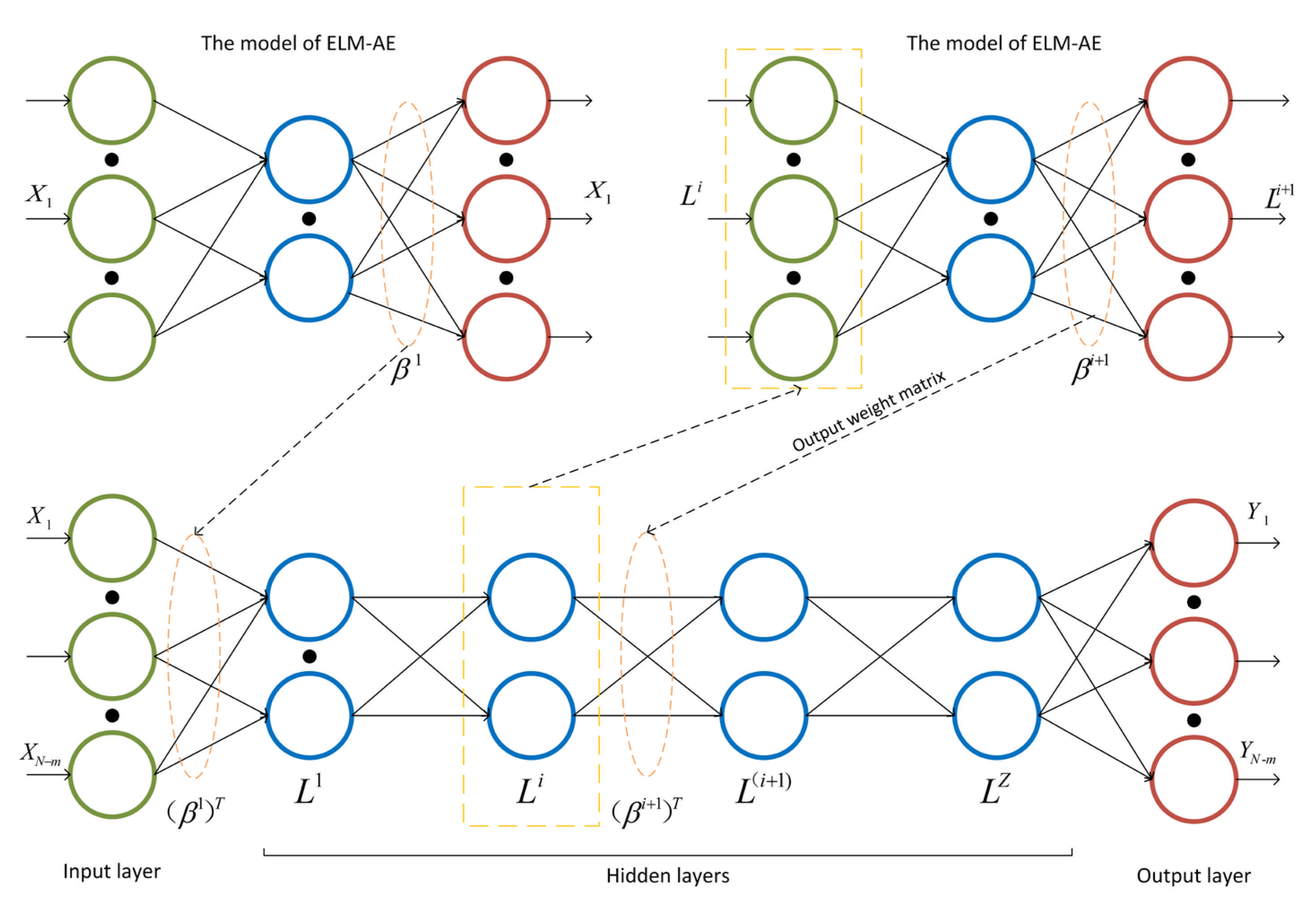
2.2. Deep Extreme Learning Machine

Deep extreme learning machine (DELM) is a derivative algorithm of ELM, which builds a multi-layer network structure by stacking extreme learning machine-automatic encoder (ELM-AE), which improves the characterization ability of the network. When ELM is faced with input and output variables with a too large amount and too high dimensionality of input data, the problem that the extreme learning machine with a single hidden layer cannot capture the effective features of the data is solved [38]. The DELM is a combination of extreme learning machine and automatic encoder to form an extreme learning machine-automatic encoder, whose structure is shown in Figure 1.

An automatic encoder (AE) is an unsupervised neural network model that can be used for feature dimensionality reduction. It has a better effect than principal component analysis (PCA) because the neural network model can extract more effective new features. In addition to feature dimensionality reduction, the new features learned by the AE can be input into the supervised learning model so that the AE can function as a feature extractor. The training goal of AE is to capture the more valuable information of the original input while approximately reconstructing the original input so that it can learn the useful characteristics of the data.

If N − m > L, ELM-AE can map high-dimensional input data to a compressed feature space, and the feature representation can be called compressed representation data; If N − m < L, ELM-AE realizes sparse expression and can convert input data from low-dimensional representation space to high-dimensional representation space. Feature representation can be called extended-dimensional data; normally, the data representation realized by N − m = L is meaningless. In summary, ELM-AE is a universal approximator, which is characterized by making the output of the network the same as the input. The constructed ELM-AE makes the weights and thresholds of hidden layer nodes randomly generated and orthogonal, thereby improving the generalization ability of ELM-AE. The ELM-AE compression expression is realized in this article. In order to further improve the generalization ability and robustness of the model, regularization parameters are introduced in the solution of the weight coefficients. The objective function is set as:

$${\mathrm{minJ}}_{ELM}=\left\{\frac{1}{2}||\beta |{|}^2+\frac{C}{2}||Y-\beta H|{|}^2\right\}$$

(2)

where C is the regularization parameter, Y is the output of the hidden layer, and H is the output matrix of the hidden layer.

For the sparse and compressed ELM-AE, taking the derivative of β in the formula and letting the objective function be 0, it can be obtained as

$$\beta ={\left(\frac{1}{C}+H^{T}H\right)}^{-1}{H}^{T}X$$

(3)

where X is the input data.

For ELM-AE, whose input dimension is equal to the coding dimension, the calculation formula is

$$\beta {=H}^{-1}X$$

(4)

$${\beta }^T\beta =I$$

(5)

where I is the identity matrix.

Each hidden layer of DELM is independent of each other. As the number of layers of the network increases, the input of the network is converted into more advanced features. After the unsupervised layer-by-layer training of DELM is over, these extracted high-level features will be used as input to train a supervised single hidden layer extreme learning machine to obtain the final result of the network. At this point, the input of ELM has become a low-dimensional high-level feature after feature extraction. The structure of DELM is shown in Figure 2.

Assuming that the model has Z hidden layers, the first output weight matrix ${\beta }^1$ is obtained from the input data X according to the ELM-AE theory, and then the feature vector $H^1$ of the hidden layer is obtained. By analogy, the output weight matrix ${\beta }^Z$ of the Z layer and the feature vector $H^Z$ of the hidden layer can be obtained. As shown in Figure 2, DELM first uses multiple ELM-AEs for unsupervised pre-training and then uses the output weights of each ELM-AE to initialize the entire DELM. In the ELM-AE training process, the input layer weights and thresholds are randomly generated orthogonal random matrices; at the same time, the ELM-AE unsupervised training process uses the least square method to update the parameters. However, only the weight parameters of the output layer will be updated in the process, and the weight and threshold of the input layer are fixed, which will cause the prediction accuracy of DELM to be affected by the random input weight and random threshold of each ELM-AE. Therefore, it is necessary to optimize these two parameters.

2.3. Deep Extreme Learning Machine Optimized by Sparrow Search Algorithm

2.3.1. Principles of Sparrow Search Algorithm

Using the global optimization ability of the sparrow search algorithm (SSA), we can find the input weight and threshold of the deep extreme learning machine when the training error is small, thereby improving the generalization ability of the deep extreme learning machine and improving the prediction accuracy of DELM.

The sparrow search algorithm was proposed by Xue et al. in 2020. The algorithm is generated by simulating the sparrow population in foraging and escaping from predators. During the foraging process of sparrows, the population can be divided into three categories, namely, discoverers, entrants, and guards. The discoverers provide foraging areas and directions for all entrants. The entrants follow the discoverers to obtain food. The identities of discoverers and entrants change dynamically. As long as a better source of food can be found, every sparrow can become a discoverer, but the proportion of discoverers and entrants in the entire population remains unchanged. The role of the guard is to spot predators. When aware of the danger, the sparrows at the edge of the group will quickly move to the safe area to obtain a better position. Sparrows in the middle of the population will move randomly to get closer to other sparrows [39].

In the sparrow search algorithm, the discoverer with a better fitness value will obtain food first in the search process. Because the discoverer is responsible for finding food for the entire sparrow population and providing foraging directions for all entrants, the discoverer can obtain a larger foraging search range than the entrants.

In the process of each iteration, the location of the discoverer is updated as described as:

$$D_{c.e}^{t+1}=\left\{\begin{array}{cc}{D}_{c.e}^t·\exp (-\frac{c}{\alpha ite{r}_{\max }}),\hfill & R_2<ST\\ D_{c.e}^t+QK,\hfill & R_2\ge ST\end{array}\right.$$

(6)

In Formula (6): t is the current number of iterations; $ite{r}_{max}$ is the maximum number of iterations; $D_{c.e}^t$ is the position information of the c-th sparrow in the e-th dimension; $\alpha$ ∈ [0, 1] is a random number; $R_2$ and ST, respectively, represent the warning value and the safety value, where $R_2$ ∈ [0, 1], ST ∈ [0.5, 1]; Q is a random number that obeys a normal distribution; K is a 1 × d matrix, where each element in the matrix is 1. When $R_2$ < ST, it means that there are no predators around the foraging environment at this time, and the discoverer can perform a wide range of search operations; when $R_2$ ≥ ST, this means that some sparrows in the population have found the predator and send alerts to others in the population. At this time, all sparrows need to fly quickly to other safe places for food.

The entrant’s location update description is:

$$D_{c.e}^{t+1}=\left\{\begin{array}{cc}{Q}_{\exp }(\frac{D_{worst}^t-D_{c.e}^t}{c^2}),& \mathrm{c}>\frac{n}{2}\\ D_F^{t+1}+|D_{c.e}^t-D_F^{t+1}|\cdot A^{+}\cdot K,& \mathrm{otherwise}\end{array}\right.$$

(7)

In Formula (7): $D_F$ is the best position occupied by the discoverer; $D_{worst}$ is the worst position; A is a 1 × d matrix, in which each element is randomly assigned a value of 1 or −1. $A^{+}=A^T{\left(A{A}^T\right)}^{-1}$, where $A^{+}$ is the pseudo-inverse matrix. When c > n/2, this indicates that the c-th entrant with a lower fitness value has no food and is very hungry. At this time, it needs to fly to other places to find food and obtain more energy.

The guards are randomly generated in the population, and their mathematical expression is:

$$D_{c.e}^{t+1}=\left\{\begin{array}{cc}{D}_{best}^t+V|D_{c.e}^t-D_{best}^t|,& f_c>f_g\\ D_{c.e}^t+O\left[\frac{|D_{c.e}^t-D_{worst}^t|}{(f_c-f_w)+\delta }\right],& f_c=f_g\end{array}\right.$$

(8)

In Formula (8): $D_{best}$ is the current global optimal position; V is the step-length control parameter, which obeys a normal distributed random number with a mean value of 0 and a variance of 1; O is a random number, which means that the direction in which the sparrow moves is also a step-length control parameter, and O ∈ [−1, 1]; $f_c$ is the fitness value of the current individual sparrow; $f_g$ and $f_w$ are the current global best and worst fitness values, respectively; $\delta$ is the smallest constant to avoid zero in the denominator. In order to simplify the process, when $f_c$ > $f_g$ means that the sparrow is at the edge of the population at this time, and it is extremely vulnerable to attack by predators; When $f_c$ = $f_g$, this indicates that the sparrows in the middle of the population are aware of the danger and need to be close to other sparrows to minimize their risk of predation. The process of the SSA-DELM model (see Figure 3 and Algorithm 1) is presented is the following segment.

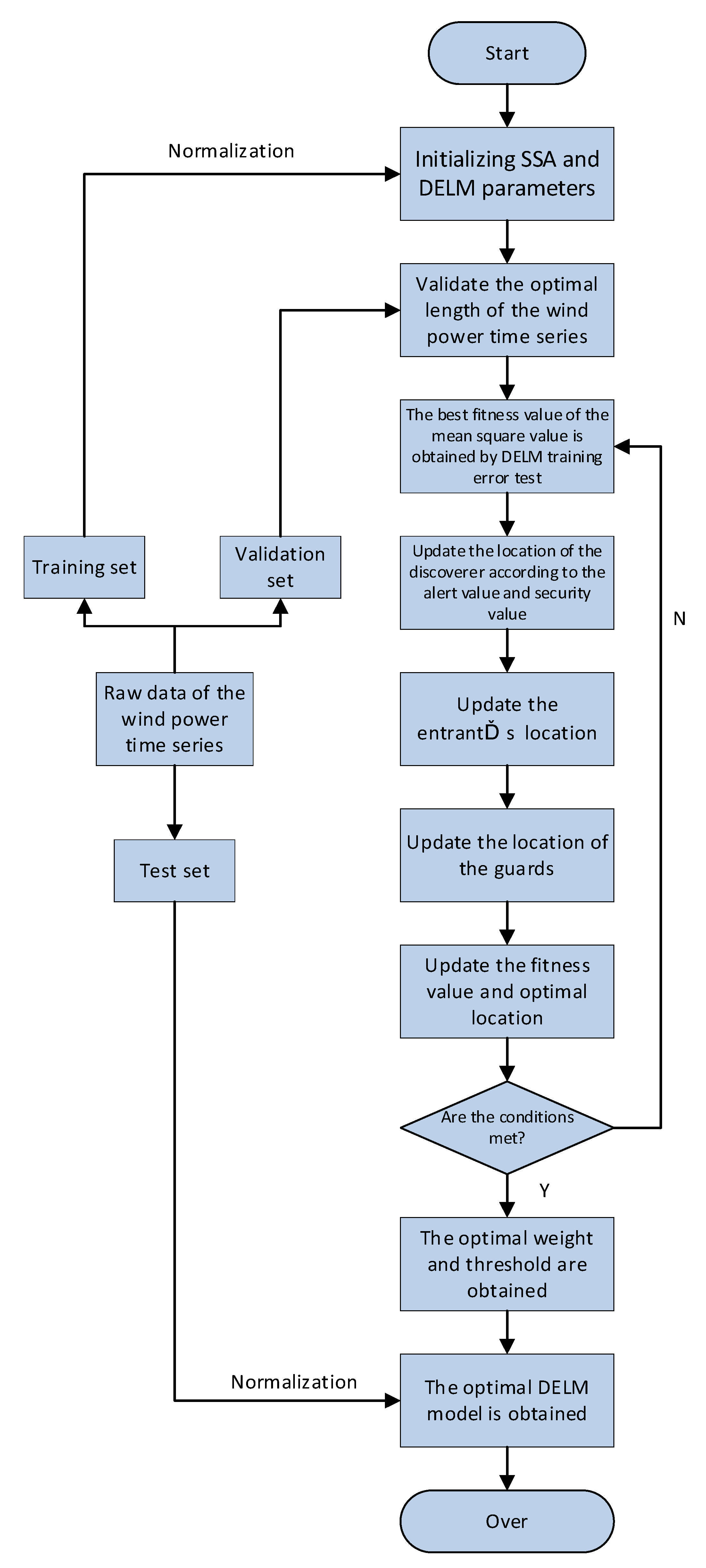
2.3.2. The Process of the SSA-DELM Model

Algorithm 1: DELM optimized by the sparrow search algorithm

Input: Population: P; Maximum number of iterations: T; Dimensions: E; The number of discoverers: DS; The number of guards: GD; The warning value: R2. Output: The best vector (solution)—Dbest 1: while (t < T) 2: Rank the fitness values and find the current best individual and the worst individual; 3: R2 = rand (0, 1) 4: for c = 1: DS 5: Use Formula (6) to update the location of the discoverers; 6: end for 7: for c = (DS + 1): P 8: Use Formula (7) to update the location of the entrants;   9: end for 10: for c = 1: GD 11: Use Formula (8) to update the location of the guards; 12: end for 13: Obtain the current new location; 14: If the new location is better than before, replace the location with the new one; 15: t = t + 1 16: end while 17: return Dbest, fg; 18: Substitute the Dbest vector into the DELM model.

3. Case Analysis

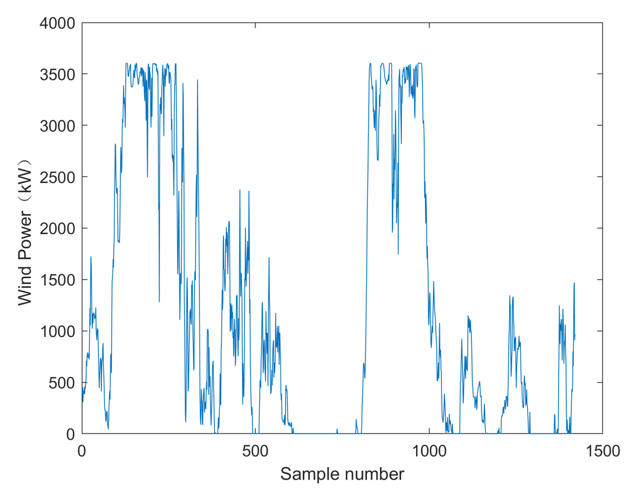
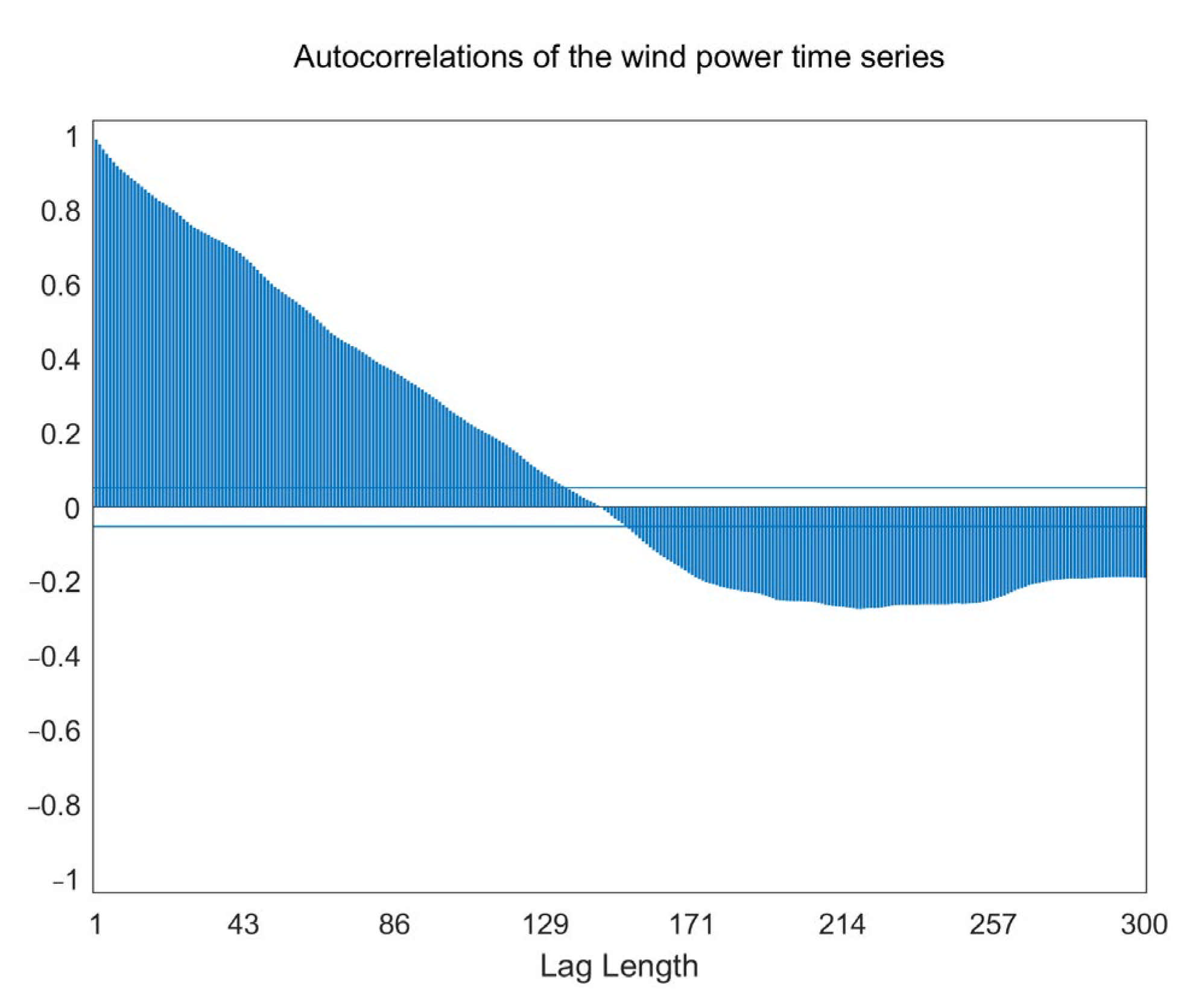
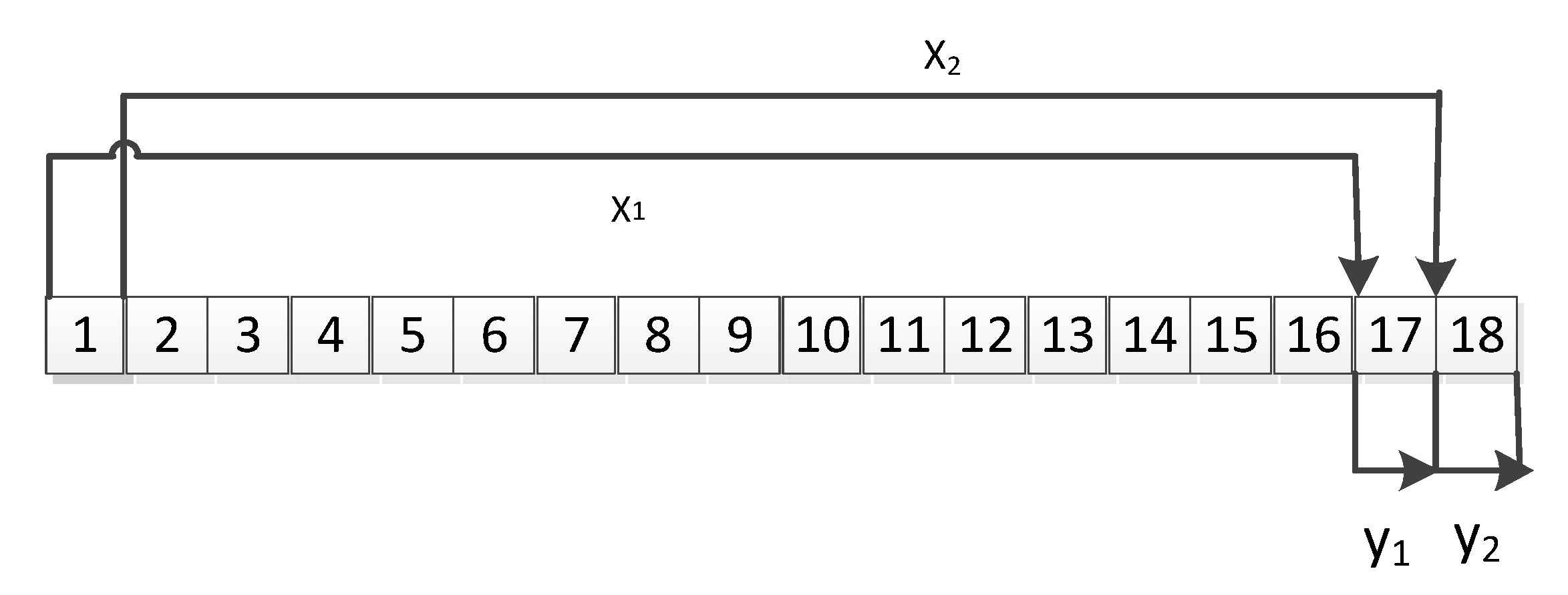
3.1. Sample Selection and Processing

In order to verify the availability and practicability of the proposed model, we take the power data of a wind farm in China from 0:00 on 1 January 2018 to 0:00 on 11 January 2018 as the data set of this paper. The data set is collected every 10 minutes by a SCADA system set in the wind turbine and the unit of wind power in kilowatts (kw). This data set contains 1420 groups of valid data.

Table 1. Five groups of data in the data set.

Sample Point	Wind Power (kW)	Wind Speed (m/s)	Wind Direction (°)
1	752.73	6.60	242.78
2	589.07	5.98	234.98
3	1109.13	7.42	235.15
4	1482.46	8.19	238.48
5	1523.43	8.27	237.03

shows five groups of data in this data set. Figure 4 shows the curve of the 10 days’ wind power. We divide the training set, test set, and validation set in a ratio of 6:2:2, which means there are 852 training sets and 284 test sets and validation sets. Autocorrelation function (ACF) refers to the linear relationship between the sequence value $x_i$ and its own lag value $x_{i+300}$ (here, the lag is set to three hundred, that is, lag = 300). The ACF diagram of the time series used in this article is shown in Figure 5.

One of the main characteristics of wind power is its uncertainty. It can be seen from Figure 4 that the wind power fluctuates in the range of 0−3600 kw, and there is no obvious periodicity and regularity in the change of wind power. This is also the main problem to be solved by analyzing and studying the internal connection of time series and realizing ultra-short-term wind power forecasting.

ACF describes the autocorrelation between one observation and another. It can be seen from Figure 5 that the ACF diagram is composed of multiple bar charts. Its abscissa is the lag order, and the ordinate is the autocorrelation coefficient. The lower the lag order, the larger the correlation coefficient and the stronger the correlation of the corresponding data. It can also be seen in Figure 5 that the change in wind power is not abrupt. Instead, there is a strong autocorrelation, which means the value to be predicted is closely related to the recent historical value. This characteristic of wind power makes it suitable for time series analysis and forecasting.

The range of input data will affect the initialization of the model. Some activation functions, including the sigmoid function, require input values that range from 0 to 1, so does the output of the network’s last node. Therefore, the normalization process is necessary. Normalization can also eliminate the influence of potential singular values. In order to improve the prediction accuracy and speed up the optimization process of SSA, we use min-max normalization to preprocess the data. The normalization function is as Formula (9) shows. The normalized time series is shown in Figure 6. It can be seen that all data are mapped in the interval [0, 1]. Inverse normalization is performed after the model outputs the results.

$$P_{tm}=\frac{P_t-P_{\min }}{P_{\max }-P_{\min }}$$

(9)

This paper will construct time sequence features based on the correlation of the data and use the time sequence features to predict the wind power at the next sample point. At the same time, the power at all sample points is predicted through rolling window prediction and compared with the actual value. Figure 7 shows the RMSE and MAE of prediction when the DELM model is used to predict time series of different lengths in the validation set, in which the horizontal axis is the length of time sequence characters, and the vertical axis is the error value.

It can be seen that the error curve shows a downward trend before the length of the time series is 16, and after this point, it starts to rise as the length of the time characteristic sequence increases. When the length of the time series is 16, the RMSE and MAE both reach the minimum values.

Formulas (10) and (11) are the calculation formulas of RMSE and MAE, respectively. The smaller values of RMSE and MAE mean better prediction accuracy of the model and vice versa. We set the length of the time sequence to 16, that is, m = 16.

$$\mathrm{RMSE}=\sqrt{\frac{{\displaystyle \sum _{k=1}^n{\left(x\left(k\right)-x_i\left(k\right)\right)}^2}}{n}}$$

(10)

$$\mathrm{MAE}=\frac{1}{n}{\displaystyle \sum _{k=1}^n|x(k)-x_i}(k)|$$

(11)

where $x\left(k\right)$ is the actual value, $x_i\left(k\right)$ is the predicted value, and $x$(k) is the average value of the actual value. From formulas (10) and (11), it can be seen that the smaller the two indicators, the closer the prediction results of the model are to reality. For a wind turbine with a maximum power generation of 3600 kW, the RMSE and MAE values are 116.4 kW and 73.5 kW, respectively, and the prediction results can serve as a suitable reference for the industry.

The data of the 1st to the 16th sample points $x_1$ are selected as the model’s first set of input to predict the power $y_1$, which is the power at the 17th sample point. Similarly, we select the data of the 2nd to 17th sample points $x_2$ as the next set of input data to predict the power $y_2$ of the 18th sample point, as shown in Figure 8.

The proposed model establishes a rolling modeling mechanism by eliminating the oldest measured wind power data and adding the latest measured wind power data in each prediction interval. In the process of model training and prediction, the 16 previous measurement values currently used will be updated in the next step, and the actual value of the current prediction will be added as the latest historical value of the next prediction.

The SSA-DELM model is used for the experiment, 70% of the experimental data is used as the training set, and the remaining 30% is used as the test set. The input variable is the wind power time series of 16 sample points, and the output variable is the wind power of the next sample point. The proposed prediction model based on SSA-DELM can accurately and effectively predict wind power in the next 10 min.

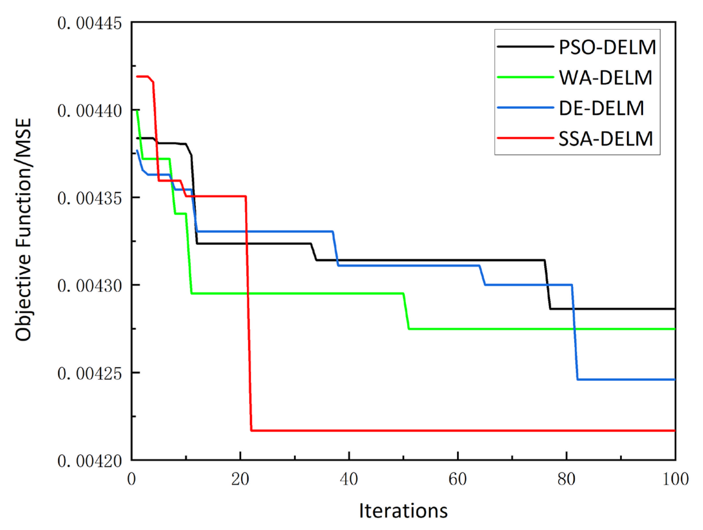
3.2. Optimizing Performance Analysis

The sparrow search algorithm has the advantages of fast iteration and strong generalization ability and can be used to optimize the DELM model. In the SSA-DELM wind power prediction model, the population size of sparrows is set to 10, and the maximum number of iterations is 100. The number of discoverers accounts for 20% of the entire population, and the safety threshold is 0.8. The sig function is selected as the activation function [40]. The iteration speeds of PSO-DELM, DELM optimized by whale algorithm (WA-DELM), DELM optimized by differential evolution algorithm (DE-DELM), and SSA-DELM are selected for comparison. The maximum number of iterations of the two models is set to 100, the objective function is the mean square error (MSE), and the Formula (12) is the calculation formula for MSE.

$$\mathrm{MSE}=\frac{1}{n}{\displaystyle \sum _{k=1}^n(x(k)-x_i}(k){)}^2$$

(12)

where$x\left(k\right)$ is the actual value and $x_i\left(k\right)$ is the predicted value. The iterative curves of the four swarm intelligence models are shown in Figure 9.

It can be seen from Figure 9 that when the sparrow search algorithm is used to optimize the DELM parameters, the global optimal solution can be found in 21 iterations. In the process of PSO optimization, the iteration curve shows that between the 31st and 77th iterations, the MSE value of the DELM model remains the same, and it is not the optimal solution at this time, which means that the optimization process has fallen into a local optimum. Similarly, whale algorithm optimization fell into a local optimum between the 10th and 50th iterations, and the optimal solution was found after 51 iterations. The iterative process of the differential evolution algorithm is relatively stable, reaching the optimum after the 82nd iteration, and there is no obvious sign of local optimum in the iterations. However, the MSE values obtained by the above three optimization algorithms are all greater than the SSA algorithm, which only requires 22 iterations to find the optimal solution. This is mainly due to the fact that the sparrow search algorithm divides the population into three categories, and each performs its own duties, which greatly improves the efficiency of optimization. From the calculation formula of MSE, it is known that the smaller the MSE, the smaller the prediction error, and the smaller the prediction accuracy of the model. In summary, it shows that SSA-DELM is more convergent and has the advantages of faster speed, higher prediction accuracy, and better model effect compared to the other four models. The effectiveness of the sparrow search algorithm used in this experiment in optimizing the DELM model is verified.

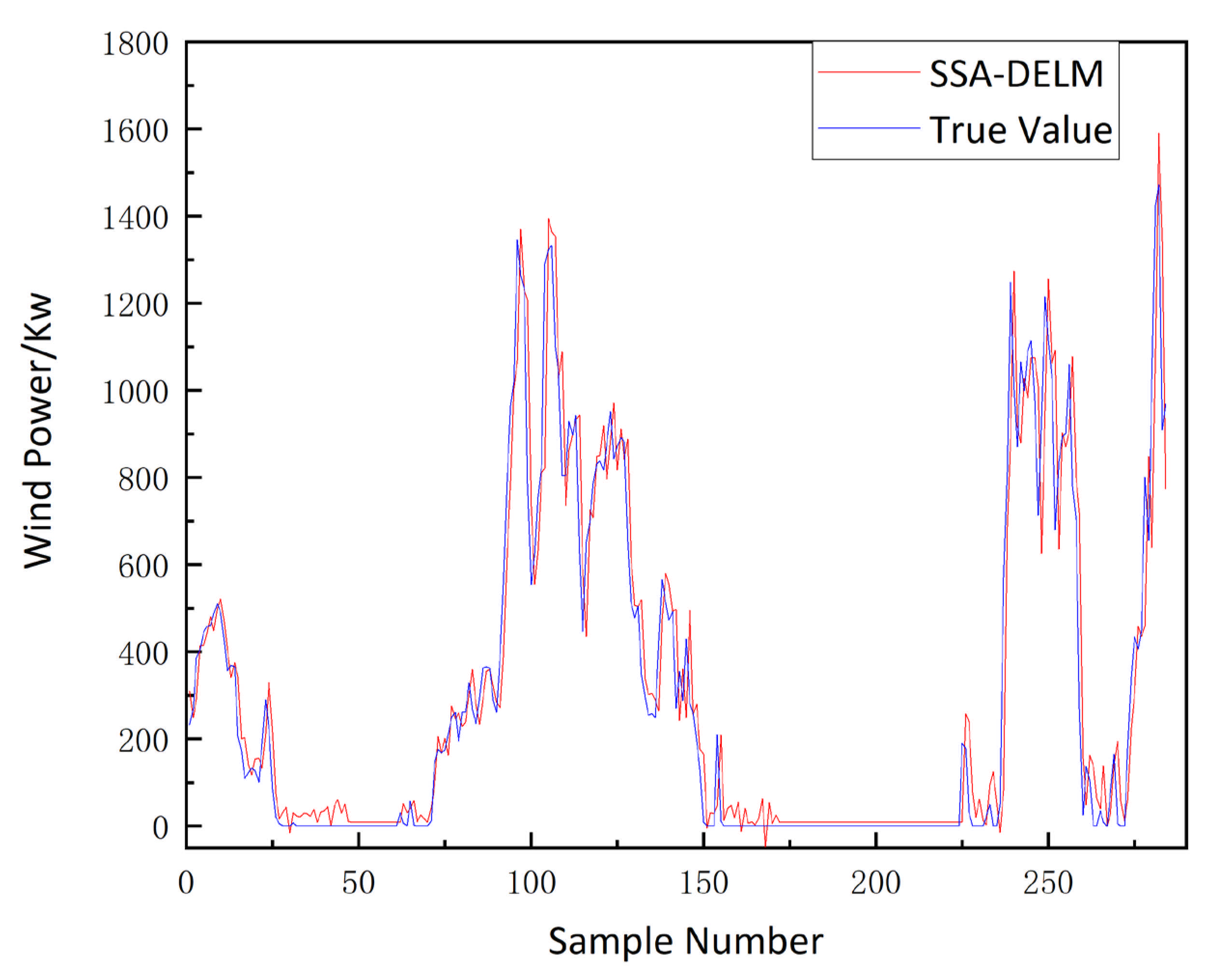
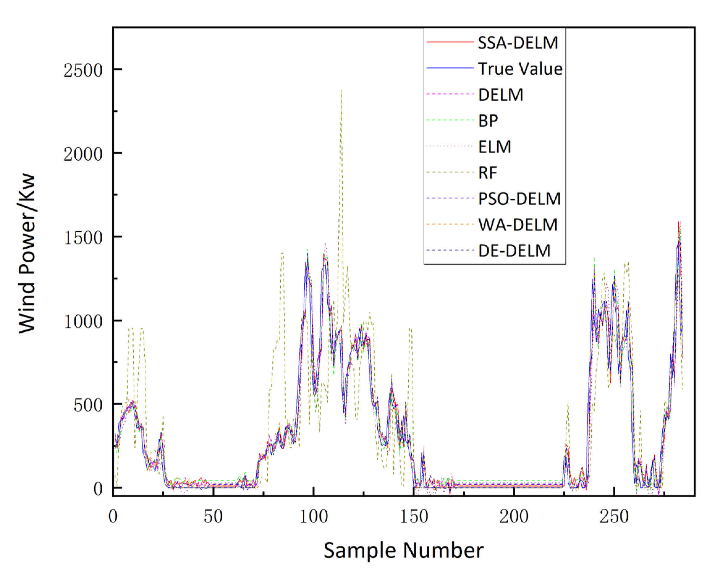
3.3. Analysis of Prediction Results

The sparrow search algorithm optimizes the DELM’s input weights and thresholds so that the SSA-DELM model has satisfactory prediction performance. The comparison of predicted results of SSA-DELM and actual data is shown in Figure 10.

It can be seen in Figure 10 that the resulting curve of the SSA-DELM model is very close to actual data. This proves that the SSA-DELM model is effective and that the prediction results are reliable.

In order to compare and verify the accuracy and effectiveness of SSA-DELM for short-term wind power prediction, seven prediction models, including backpropagation (BP) neural network, random forest (RF), ELM, DELM, PSO-DELM, DE-DELM, and WA-DELM, were also established for simulation and comparative analysis. The results are shown in Figure 11.

The comparison in Figure 11 shows that most of these models can make a rough forecast of wind power, but their accuracy varies. Among them, the ultra-short-term wind power prediction curve of the SSA-DELM model is closest to the actual power curve. In other words, the prediction accuracy of SSA-DELM is the highest.

To further verify the accuracy of the wind farm power prediction model, the error indicators (RMSE and MAE) and the determination coefficient R² are used to evaluate the SSA-DELM prediction model [41]. Formula (13) is R², the calculation formula, and the results are shown in

Table 2. Comparison of error indicators of different prediction models.

	RMSE	MAE	R²
RF	285.881	159.592	0.601
BP	132.592	94.360	0.826
ELM	128.356	77.146	0.893
DELM	121.268	73.917	0.903
DE-DELM	117.473	72.875	0.911
PSO-DELM	116.243	72.689	0.915
WA-DELM	116.153	72.467	0.921
SSA-DELM	115.446	69.803	0.927

. Error analysis and coefficient of determination are important tools to test whether the model is effective.

$$R^2=\frac{{\displaystyle \sum _{k=1}^n{\left(x_i(k)-\overline{x}(k)\right)}^2}}{{\displaystyle \sum _{k=1}^n{\left(x(k)-\overline{x}(k)\right)}^2}}$$

(13)

where$x\left(k\right)$ is the actual value, $x_i\left(k\right)$ is the predicted value, and $\overline{x}\left(k\right)$ is the average of the actual value.

It can be seen from Table 2 that the three error indicators of the SSA-DELM model are the best in all the models above.

Compared with the DELM model, the combined model of SSA optimized DELM used in this article reduces the above two indicators of RMSE and MAE by 1.485% and 1.669%, respectively, and increases R² by 1.086%, which illustrates the optimization of the SSA algorithm is effective. Compared with PSO-DELM, the above two indicators of RMSE and MAE are reduced by 0.404% and 1.122%, respectively, and R² is increased by 0.543% compared with PSO-DELM. Compared with DE-DELM, PSO-DELM, and WA-DELM, the model proposed in this paper reduces RMSE indicators by 1.726%, 0.686%, and 0.609%, respectively. The MAE indexes are reduced by 4.215%, 3.970%, and 3.676%, respectively. The R² indexes of the model are increased by 1.726%, 1.294%, and 0.647%, respectively. It shows that the sparrow search algorithm used in this paper to optimize DELM is better than the other four algorithms to optimize DELM. Compared with RF, BP, ELM, and SSA-ELM, DELM reduced the RMSE by 57.834%, 12.673%, 7.861%, and 6.715%, respectively. Compared with RF, BP, ELM, and SSA-ELM, DELM reduces the MAE by 54.466%, 23.662%, 12.075%, and 10.218%, respectively. Compared with RF, BP, ELM, and SSA-ELM, DELM has increased R² by 29.638%, 3.842%, 1.098%, and 0.439%, respectively. Based on the above analysis, it can be concluded that the SSA algorithm can indeed optimize the parameters of the DELM prediction model. Therefore, the SSA-DELM prediction model can be established and applied to the short-term wind power prediction of actual wind farms. The prediction results show that the proposed wind power prediction method has high prediction accuracy, which provides a new way for short-term wind power prediction.

4. Conclusions

Aiming at the problem of poor prediction accuracy of existing wind power forecasting models, this paper proposes a wind power forecasting method based on SSA-DELM. Through the analysis of measured wind power data, the following conclusions are obtained:

(1)

The method based on the DELM model to optimize time series’ length for rolling sequence prediction can meet the requirements of the proposed SSA-DELM model to accomplish higher training efficiency;

(2)

The SSA-DELM wind power prediction model proposed in this paper has better performance than the four models of RF, BP, ELM, and SSA-ELM in terms of MAE, RMSE, and R². Compared with traditional DELM, the combined model of SSA optimized DELM proposed in this article reduces the above RMSE and MAE by 4.801% and 5.566%, respectively, and increases R² by 2.589%. Compared with DE-DELM, PSO-DELM and WA-DELM, the model proposed in this paper reduces RMSE, MAE and increases R² by 1.726%, 0.686%, 0.609%; 4.215%, 3.970%, 3.676%; 1.726%, 1.294%, and 0.647%, respectively.

(3)

In the current wind power forecasting model, the input and output samples are normalized power time series, which is sensitive to noise and abnormal data. In the future, we will consider using advanced data processing methods to structure the original data, reduce noise, and then separately predict the sequence obtained from the decomposition and fuse the prediction results to improve the robustness of the model.

References

1. Oh, E.; Son, S.-Y. Theoretical energy storage system sizing method and performance analysis for wind power forecast uncertainty management. Renew. Energy 2020, 155, 1060–1069. [Google Scholar] [CrossRef]
2. Zhou, M.; Wang, B.; Guo, S.; Watada, J. Multi-objective prediction intervals for wind power forecast based on deep neural networks. Inf. Sci. 2020, 550, 207–220. [Google Scholar] [CrossRef]
3. Santhosh, M.; Venkaiah, C.; Vinod Kumar, D.M. Review on Key Technologies and Applications in Wind Power Forecasting. High Volt. Eng. 2021, 47, 1129–1143. [Google Scholar]
4. Huang, B.; Liang, Y.; Qiu, X. Wind Power Forecasting Using Attention-Based Recurrent Neural Networks: A Comparative Study. IEEE Access 2021, 9, 40432–40444. [Google Scholar] [CrossRef]
5. Han, L.; Jing, H.; Zhang, R.; Gao, Z. Wind power forecast based on improved Long Short Term Memory network. Energy 2019, 189, 116300. [Google Scholar] [CrossRef]
6. Wu, Q.; Lin, H. Short-Term Wind Speed Forecasting Based on Hybrid Variational Mode Decomposition and Least Squares Support Vector Machine Optimized by Bat Algorithm Model. Sustainability 2019, 11, 652. [Google Scholar] [CrossRef] [Green Version]
7. Yu, Y.; Yang, M.; Han, X.; Zhang, Y.; Ye, P. A Regional Wind Power Probabilistic Forecast Method Based on Deep Quantile Regression. IEEE Trans. Ind. Appl. 2021, 57, 4420–4427. [Google Scholar] [CrossRef]
8. Hong, D.; Ji, T.; Li, M.; Wu, Q. Ultra-short-term forecast of wind speed and wind power based on morphological high frequency filter and double similarity search algorithm. Int. J. Electr. Power Energy Syst. 2018, 104, 868–879. [Google Scholar] [CrossRef]
9. Li, Q.; Zhang, X.Y.; Ma, T.J.; Ma, T.; Wang, H.; Yin, H.S. Multi-step Ahead Ultra-short Term Forecasting of Wind Power Based on ECBO-VMD-WKELM. Power Syst. Technol. 2021, 3, 1–14. [Google Scholar]
10. Li, J.; Li, M. Prediction of ultra-short-term wind power based on BBO-KELM method. J. Renew. Sustain. Energy 2019, 11, 056104. [Google Scholar] [CrossRef]
11. Yang, M.; Zhang, L.; Cui, Y.; Yang, Q.; Huang, B. The impact of wind field spatial heterogeneity and variability on short-term wind power forecast errors. J. Renew. Sustain. Energy 2019, 11, 033304. [Google Scholar] [CrossRef] [Green Version]
12. An, G.; Jiang, Z.; Cao, X.; Liang, Y.; Zhao, Y.; Li, Z.; Dong, W.; Sun, H. Short-term Wind Power Prediction Based On Particle Swarm Optimization-Extreme Learning Machine Model Combined with Adaboost Algorithm. IEEE Access 2021, 9, 1. [Google Scholar] [CrossRef]
13. Li, L.-L.; Zhao, X.; Tseng, M.-L.; Tan, R.R. Short-term wind power forecasting based on support vector machine with improved dragonfly algorithm. J. Clean. Prod. 2019, 242, 118447. [Google Scholar] [CrossRef]
14. Zhao, H.; Zhao, H.; Guo, S. Short-Term Wind Electric Power Forecasting Using a Novel Multi-Stage Intelligent Algorithm. Sustainability 2018, 10, 881. [Google Scholar] [CrossRef] [Green Version]
15. Dolatabadi, A.; Abdeltawab, H.; Mohamed, Y.A. Short-term Wind Power Prediction Based on Dynamic Cluster Division and BLSTM Deep Learning Method. High Volt. Eng. 2021, 47, 1195–1203. [Google Scholar]
16. Alhaidari, F.; AlMotiri, S.H.; Al Ghamdi, M.A.; Khan, M.A.; Rehman, A.; Abbas, S.; Khan, K.M.; Rahman, A.U. Intelligent Software-Defined Network for Cognitive Routing Optimization using Deep Extreme Learning Machine Approach. Comput. Mater. Contin. 2021, 67, 1269–1285. [Google Scholar] [CrossRef]
17. Nayak, D.R.; Das, D.; Dash, R.; Majhi, S.; Majhi, B. Deep extreme learning machine with leaky rectified linear unit for multiclass classification of pathological brain images. Multimed. Tools Appl. 2019, 79, 15381–15396. [Google Scholar] [CrossRef]
18. Zhao, F.X.; Liu, Y.X.; Huo, K. A radar target classification algorithm based on dropout constrained deep extreme learning machine. J. Radars 2018, 7, 613–621. [Google Scholar]
19. Khatab, Z.E.; Hajihoseini, A.; Ghorashi, S.A. A Fingerprint Method for Indoor Localization Using Autoencoder Based Deep Extreme Learning Machine. IEEE Sens. Lett. 2017, 2, 1–4. [Google Scholar] [CrossRef]
20. Suzuki, G.; Takahashi, S.; Ogawa, T.; Haseyama, M. Team Tactics Estimation in Soccer Videos Based on a Deep Extreme Learning Machine and Characteristics of the Tactics. IEEE Access 2019, 7, 153238–153248. [Google Scholar] [CrossRef]
21. Yin, Z.; Zhang, J. Task-generic mental fatigue recognition based on neurophysiological signals and dynamical deep extreme learning machine. Neurocomputing 2018, 283, 266–281. [Google Scholar] [CrossRef]
22. Lu, P.; Ye, L.; Sun, B.; Zhang, C.; Zhao, Y.; Teng, J. A New Hybrid Prediction Method of Ultra-Short-Term Wind Power Forecasting Based on EEMD-PE and LSSVM Optimized by the GSA. Energies 2018, 11, 697. [Google Scholar] [CrossRef] [Green Version]
23. Wu, J.; Zhou, T.; Li, T. A Hybrid Approach Integrating Multiple ICEEMDANs, WOA, and RVFL Networks for Economic and Financial Time Series Forecasting. Complexity 2020, 2020, 1–17. [Google Scholar] [CrossRef]
24. Zhang, Y.; Zhang, J.; Luo, L.; Gao, X. Optimization of LMBP high-speed railway wheel size prediction algorithm based on improved adaptive differential evolution algorithm. Int. J. Distrib. Sens. Netw. 2019, 15, 348. [Google Scholar] [CrossRef]
25. Lei, B.Y.; Wang, Z.C.; Su, Y.Q.; Sun, W.Z.; Yang, L.Y. Research on Short-term Load Forecasting Method Based on EEMD-CS-LSSVM. Proc. CSU-EPSA 2021, 3, 1–7. [Google Scholar]
26. Gómez, J.L.; Martínez, A.O.; Pastoriza, F.T.; Garrido, L.F.; Álvarez, E.; García, J.O. Photovoltaic Power Prediction Using Artificial Neural Networks and Numerical Weather Data. Sustainability 2020, 12, 10295. [Google Scholar] [CrossRef]
27. Ahmadi, M.H.; Ahmadi, M.A.; Nazari, M.A.; Mahian, O.; Ghasempour, R. A proposed model to predict thermal conductivity ratio of Al2O3/EG nanofluid by applying least squares support vector machine (LSSVM) and genetic algorithm as a connectionist approach. J. Therm. Anal. Calorimetry. 2019, 135, 271–281. [Google Scholar] [CrossRef]
28. Ahmadi, M.H.; Tatar, A.; Nazari, M.A.; Ghasempour, R.; Chamkha, A.J.; Yan, W.M. Applicability of connectionist methods to predict thermal resistance of pulsating heat pipes with ethanol by using neural networks. Int. J. Heat Mass Transf. 2018, 126, 1079–1086. [Google Scholar] [CrossRef]
29. Ahmadi, M.H.; Sadeghzadeh, M.; Raffiee, A.H.; Chau, K.W. Applying GMDH neural network to estimate the thermal resistance and thermal conductivity of pulsating heat pipes. Eng. Appl. Comput. Fluid Mech. 2019, 13, 327–336. [Google Scholar] [CrossRef] [Green Version]
30. Yue, X.Y.; Peng, X.A.; Lin, L. Short-term Wind Power Forecasting Based on Whales Optimization Algorithm and Support Vector Machine. Proc. CSU-EPSA 2020, 32, 146–150. [Google Scholar]
31. Li, N.; He, F.; Ma, W.; Wang, R.; Zhang, X. Wind Power Prediction of Kernel Extreme Learning Machine Based on Differential Evolution Algorithm and Cross Validation Algorithm. IEEE Access 2020, 8, 68874–68882. [Google Scholar] [CrossRef]
32. Devi, A.S.; Maragatham, G.; Boopathi, K.; Rangaraj, A.G. Hourly day-ahead wind power forecasting with the EEMD-CSO-LSTM-EFG deep learning technique. Soft Comput. 2020, 24, 12391–12411. [Google Scholar] [CrossRef]
33. Yuan, J.; Zhao, Z.; Liu, Y.; He, B.; Wang, L.; Xie, B.; Gao, Y. DMPPT Control of Photovoltaic Microgrid Based on Improved Sparrow Search Algorithm. IEEE Access 2021, 9, 16623–16629. [Google Scholar] [CrossRef]
34. Zhu, Y.; Yousefi, N. Optimal parameter identification of PEMFC stacks using Adaptive Sparrow Search Algorithm. Int. J. Hydrogen Energy 2021, 46, 9541–9552. [Google Scholar] [CrossRef]
35. Liu, T.; Yuan, Z.; Wu, L.; Badami, B. Optimal brain tumor diagnosis based on deep learning and balanced sparrow search algorithm. Int. J. Imaging Syst. Technol. 2021, 12, 21. [Google Scholar] [CrossRef]
36. Tuerxun, W.; Chang, X.; Hongyu, G.; Zhijie, J.; Huajian, Z. Fault Diagnosis of Wind Turbines Based on a Support Vector Machine Optimized by the Sparrow Search Algorithm. IEEE Access 2021, 9, 69307–69315. [Google Scholar] [CrossRef]
37. Sulandri, S.; Basuki, A.; Bachtiar, F.A. Metode Deteksi Intrusi Menggunakan Algoritme Extreme Learning Machine dengan Correlation-based Feature Selection. J. Teknol. Inf. Dan Ilmu Kompʹut. 2021, 8, 103–110. [Google Scholar] [CrossRef]
38. Inam, A.; Zhulim, S.A.; Din, S.U.; Atta, A.; Naaseer, I.; Siddiqui, S.Y.; Khan, M.A. Detection of COVID-19 Enhanced by a Deep Extreme Learning Machine. Intell. Autom. Soft Comput. 2021, 27, 701–712. [Google Scholar] [CrossRef]
39. Wang, H.R.; Xian, Y. Optimal configuration of distributed generation based on sparrow search algorithm. IOP Conference Series. Earth Environ. Sci. 2021, 647, 012053. [Google Scholar]
40. Rehman, A.; Athar, A.; Khan, M.A.; Abbas, S.; Fatima, A.; Rahman, A.U.; Saeed, A. Modelling, simulation, and optimization of diabetes type II prediction using deep extreme learning machine. J. Ambient. Intell. Smart Environ. 2020, 12, 125–138. [Google Scholar] [CrossRef]
41. Qin, G.; Yan, Q.; Zhu, J.; Xu, C.; Kammen, D. Day-Ahead Wind Power Forecasting Based on Wind Load Data Using Hybrid Optimization Algorithm. Sustainability 2021, 13, 1164. [Google Scholar] [CrossRef]
Figure 1. Structure diagram of ELM-AE.
Sustainability 13 10453 g001
Figure 2. Structure diagram of DELM.
Sustainability 13 10453 g002
Figure 3. The flow chart of the SSA-DELM model.
Sustainability 13 10453 g003
Figure 4. Actual wind power.
Sustainability 13 10453 g004
Figure 5. Autocorrelations of the wind power time series.
Sustainability 13 10453 g005
Figure 6. The normalized wind power time series.
Sustainability 13 10453 g006
Figure 7. Comparison of errors when predicting different lengths of time series.
Sustainability 13 10453 g007
Figure 8. Rolling sequence prediction.
Sustainability 13 10453 g008
Figure 9. Comparison of optimization fitness curves of SSA-DELM and other optimized models.
Sustainability 13 10453 g009
Figure 10. Comparison between actual power with the predicted values of SSA-DELM.
Sustainability 13 10453 g010
Figure 11. Comparison of different models’ prediction results.
Sustainability 13 10453 g011