Article

A Novel Analytical Approach for Optimal Placement and Sizing of Distributed Generations in Radial Electrical Energy Distribution Systems

by
Sasan Azad
1,
Mohammad Mehdi Amiri
1,
Morteza Nazari Heris
2,*,
Ali Mosallanejad
1 and
Mohammad Taghi Ameli
1
1
Faculty of Electrical Engineering, Shahid Beheshti University, Tehran 0098, Iran
2
Department of Architectural Engineering, Pennsylvania State University, State College, PA 16802, USA
*
Author to whom correspondence should be addressed.
Sustainability 2021, 13(18), 10224; https://doi.org/10.3390/su131810224
Submission received: 2 August 2021 / Revised: 7 September 2021 / Accepted: 7 September 2021 / Published: 13 September 2021
(This article belongs to the Special Issue Energy Storage Technologies in Future Energy Systems)

Abstract

:
Considering the strong influence of distributed generation (DG) in electric distribution systems and its impact on network voltage losses and stability, a new challenge has appeared for such systems. In this study, a novel analytical algorithm is proposed to distinguish the optimal location and size of DGs in radial distribution networks based on a new combined index (CI) to reduce active power losses and improve system voltage profiles. To obtain the CI, active power losses and voltage stability indexes were used in the proposed approach. The CI index with sensitivity analysis was effective in decreasing power losses and improving voltage stability. Optimal DG size was determined based on a search algorithm to reduce active power losses. The considered scheme was examined through IEEE 12-bus and 33-bus radial distribution test systems (RDTS), and the obtained results were compared and validated in comparison with other available methods. The results and analysis verified the effectiveness of the proposed algorithm in reducing power losses and improving the distribution system voltage profiles by determining the appropriate location and optimal DG size. In IEEE 12 and 33 bus networks, the minimum voltage increased from 0.9434 p.u and 0.9039 p.u to 0.9907 p.u and 0.9402 p.u, respectively. Additionally, the annual cost of energy losses decreased by 78.23% and 64.37%, respectively.

1. Introduction

Nowadays, the need for electricity consumption has increased, considering the increment of domestic, industrial, commercial, and agricultural consumption due to the growth of the world’s population and economic development. By investing in power plant structures, the development of transmission and distribution lines can meet the demand for electricity. However, investing in these sectors, in addition to requiring a lot of time, imposes huge costs on governments and the electricity industry. If distributed generation resources supply a part of consumers’ electricity, it will significantly reduce these costs. Despite the advantages of installing distributed generation (DG) resources, their challenges and technical barriers need to be addressed.
In addition to having advantages such as voltage profile improvement [1], reduction of losses [2], increased reliability [3], and reduced overall harmonic distortion of voltage [1], DG construction has requirements that need to be considered. By installing DG, the network becomes an active network, and parameters such as network voltage profile and stability should be paid more attention. One of the issues that must be mentioned is the better optimization technique for DG placement in the distribution system. Putting DG in a non-optimal way in the distribution system may weaken voltage stability, reduce power quality, and increase network losses [4]. Therefore, the best location and size for DG installation should be selected for maximum and efficient DG installation utilization [5]. Numerous articles have so far examined the optimal location of DG. These articles are generally divided into two types. The first type is articles that are based on mathematical-based analytical methods, and the second type uses meta-innovative methods. In the following section, different articles from both types are examined.

1.1. Analytical Methods

In [6], the optimal DG location was obtained using a new voltage stability index (VSI), and its optimal size was based on the reduction of active losses. The authors also investigated the effect of load increase on optimal DG placement. The authors in [7] used a new methodology to optimize DG placement using continuous power flow. In this reference, the buses with lower voltage safety levels were first identified, and the DG was installed in place of those buses. The effect of DG location on voltage stability and loss reduction has also been investigated. In [8], using voltage stability techniques, a method for optimal DG placement in distribution systems was presented. The voltage stability technique was based on modal analysis and continuous power flow. Additionally, the objective function was to reduce the voltage stability limit and minimize network losses. In [9], the optimal placement of DG was discussed based on increasing voltage stability and reducing network losses simultaneously with the introduction of a new method. In this method, the vulnerable buses are first selected in terms of voltage stability using bifurcation analysis as suitable buses for DG installation. Then, the number of DGs is selected to place the bus voltage within the allowable range, and finally, the optimal size of the DGs is obtained using the dynamic programming search method. In [10], the authors used the power stability index (PSI), a measure of voltage stability, as a benchmark for installing DG. The optimal DG size was also selected based on the reduction of network power losses. The use of the proposed algorithm in DG placement improved the voltage profile and reduced power losses. The simulation results were compared with the golden section search algorithm and validated. The optimal placement of DG units using an improved analytical method and a loss sensitivity factor method was presented in [2]. In [11], a new analysis index was presented to locate and determine the optimal size of DG. The proposed index is a combination of the voltage stability index, the loss sensitivity factor, and reliability-based factors. The DG placement index (DGPI), which is presented in this article to select the optimal DG installation location, is expressed as the weighted sum of the mentioned indicators. In the studied networks, each bus with the highest DGPI value is selected as a suitable place to install DG. The optimal size of DG is also selected so that the DGPI value has the lowest value. In [8], a DG placement problem was solved based on voltage stability analysis as a security measure. Modal analysis and continuous power flow were used in a hierarchal placement algorithm. Additionally, a modified equivalent reactive compensation method was proposed to provide a priority list of DG locations for compensating reactive power during reactive power shortages.

1.2. Meta-Innovative Methods

In [12], the particle swarm optimization (PSO) algorithm was used to optimize DG units to reduce power losses and improve voltage profiles. In [13], the invasive weed optimization algorithm was used for optimal DG placement. In this reference, the loss sensitivity factor was used to create the priority list for DG installation. The whale optimization algorithm (WOA) was used to place DG optimally as a multi-objective in [4]. Target functions included minimizing energy losses and operating costs as well as improving voltage profiles. In [14], the modified teaching–learning based optimization (MOTLBO) algorithm was used to optimize the DG units. In [15], DG optimization was performed by considering load and generation uncertainty using a genetic algorithm (GA). Load and generation uncertainty were modeled using a fuzzy-based approach. In [16], the authors presented a new algorithm that combined genetic and SA algorithms to optimize the placement of DG. In this reference, a numerical example shows the proposed algorithm’s superiority over the simple genetic algorithm. In [17], ant colony optimization (ACO) and artificial bee colony (ABO) algorithms have solved locating and determining DG size. In this paper, the problem is modeled on statistics and probabilities, and the uncertainties in planning are taken into account. In [18], the authors suggested using the bacterial foraging optimization (BFO) algorithm to solve the DG optimal placement problem. The authors in [19] used quantum-inspired particle swarm optimization (Q-PSO) for the optimal allocation of distributed generation units. In [20], a hybrid genetic particle swarm optimization algorithm for the optimal allocation of distributed generation was developed. This paper aimed to reduce active and reactive power losses and voltage regulations in the system. In [21], a new method called Harris Hawks optimization was used to optimally locate and determine the capacity of distributed generation units in a radial distribution network. In this method, the authors aimed to minimize lost power, and they compared the performance of this method with similar methods of heuristic optimization. In [22], a new hybrid method was used to locate and determine the optimal size of DG, with the aim of reducing power losses. The combined technique was the continuous execution of both the grasshopper optimization algorithm (GOA) and the cuckoo search (CS). In this paper, GOA optimization behavior was improved using the CS technique. In [23], modified moth flame optimization (MMFO) was proposed to locate and determine the optimal size of DG. The purpose of this paper was to minimize the cost of operating the entire network by minimizing active power losses, bus voltage deviations, the cost of operating the DG, and the cost of emissions.
The main motivation of this work is to provide a new and simple analytical method for the optimal placement and sizing of DG. In this paper, we have tried to present a simple but efficient method in which voltage stability and active power loss are considered together; hence, a voltage stability index (VSI) and an active power losses index (APLI) are presented to specify the optimal location of DG. The VSI, from a mathematical point of view, is obtained by considering the sensitivity of the voltage to active power. The combination of the two proposed indicators is used as a combined index (CI) to determine the optimal location of DG, reduce active power losses, and increase network voltage stability. By implementing the DG units in power system buses, the bus that simultaneously impacts the system through a reduction of active power losses and an increase in network voltage stability has the largest CI and is selected as the candidate bus. By selecting the candidate bus, the DG size is determined by the search algorithm in order to reduce active power losses and observe the allowable voltage range. The proposed method is tested on IEEE 12-bus [24] and 33-bus [25] RDTSs for unity power factor (pf), 0.9 lagging, and optimal power factor (OPF). Then, the results of the combined power loss sensitivity (CPLS) method [26], the VSI method [6], and the index vector (IV) method [26] are compared in unity and the 0.9 lagging power factor.
The structure of the paper is as follows. In Section 2, the formulation of the problem is presented. In this section, a new analytical method is used for optimal DG placement. In Section 3, the discussion and simulation results are reviewed, and, finally, in Section 4, the paper’s overall conclusion is discussed.

2. Problem Formulation

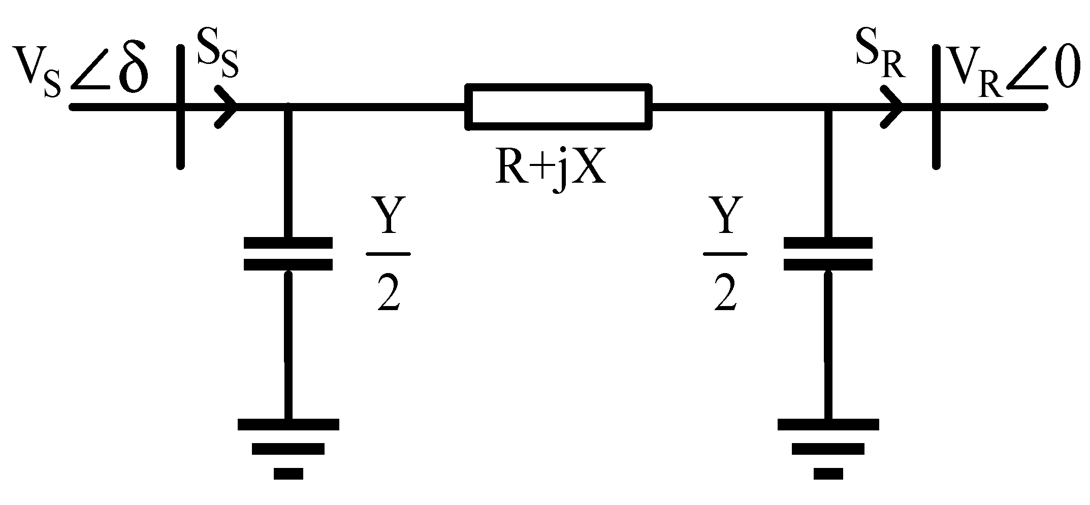
2.1. Mathematical Model of the Proposal Indicators for Optimal DG Placement

Determining the optimal DG location requires methods that reduce distribution network losses and costs while considering voltage stability and network security. To specify the proper and optimal location placement of DG, two indicators of voltage stability assessment and reduction of active losses are presented in the current work. From a mathematical point of view, the voltage stability assessment index is obtained by considering the power system’s voltage collapse characteristics and can provide a comprehensive assessment of network voltage stability status.

2.1.1. New Voltage Stability Index (NVSI)

The mathematical model of the considered VSI for DG placement is presented in this section. The system studied is shown in Figure 1. The proposed index is obtained using the transmission power in lines and a quadratic voltage equation based on the ABCD parameters of the transmission line. The line capacitor increases with increasing line length and cannot be ignored; for this reason, in addition to the impedance of lines, the line’s capacitance is also considered in the ABCD parameters. Therefore, the proposed index, considering all conditions of transmission lines, performs a voltage stability assessment. The NVSI is modeled as follows:
V S = A V R + B I R I S = C V R + D I R
By representing the above equations as a matrix, we have:
[ V S I S ] = [ A B C D ] [ V R I R ] = [ 1 + Y Z 2 Z Y ( 1 + Y Z 2 ) 1 + Y Z 2 ] [ V R I R ]
If we have
A = | A | θ A , B = | B | θ B , C = | C | θ C , D = | D | θ D
Additionally, the values of V S   and V R   are equal to:
V S = | V S | δ , V R = | V R | 0
In the following, we first calculate the flow at the end of the line:
I R = P R j Q R V R * = P R j Q R V R 0
Using (2), the voltage at the beginning of the line can be obtained as follows:
V S δ = A θ A × V R 0 + B θ B × I R = A θ A × V R 0 + B θ B × P R j Q R V R 0
By multiplying the sides of (8) in V R   ,   we have:
V S V R δ = A θ A × V R 2 + B θ B × ( P R j Q R )
Separate the real and imaginary parts of (5), and we will be equal in placing the real parts of the sides:
V R 2 A cos ( θ A ) V R V S cos ( δ ) + ( P R B cos ( θ B ) + Q R B sin ( θ B ) ) = 0
Voltage sensitivity to active power of the receiving side, according to (6), is equal to:
d V R d P R = B 2 V R A cos ( θ A ) cos ( θ B ) V S cos ( δ ) cos ( θ B )
The condition for the system to remain stable is that (11) is negative. B is always positive, so we have:
2 V R A cos ( θ A ) cos ( θ B ) V S cos ( δ ) cos ( θ B ) > 0
Therefore, according to (8), the following inequality must always be maintained to maintain voltage stability.
2 V R A cos ( θ A ) V S cos ( δ ) > 1
Due to (9), the voltage stability index is defined as follows:
N V S I = ( 2 2 V R A cos ( θ A ) V S cos ( δ ) )
The proposed index varies between zero, which indicates the state of no-load, and one, which indicates the state of voltage collapse. How to get the boundary values is as follows:
V S = A V R + B I R I S = C V R + D I R
In no-load conditions, where I R = 0 ,   we have:
V S = A V R δ = θ A
The index’s value is obtained by placing (12) in (10) ,   N V S I = 0 , which is the lower limit of the proposed index.
To obtain the upper limit of the proposed index, the value of the index at the point of voltage collapse is used in a way that when we approach the point of instability on the P V   curve, the value of d V R d P R   tends to infinity, then:
d V R d P R =
2 V R A cos ( θ A ) cos ( θ B ) V S cos ( δ ) cos ( θ B ) = 0
2 V R A cos ( θ A ) = V S cos ( δ )
By placing (15) in (10), the index’s value is obtained,   N V S I = 1 , which is the upper limit of the proposed index. According to (10), if we show the number of lines with j, the value of the NVSI for each line is obtained as follows:
N V S I j = ( 2 2 V R j A j cos ( θ A j ) V S j cos ( δ j ) )
To have a comprehensive index to voltage stability assessment of the entire system, the overall new voltage stability index (ONVSI) is defined as follows:
O N V S I i = j = 1 l N V S I j O N V S I initial
where O N V S I initial   is the sum of the index values of lines without DG installation.

2.1.2. Active Power Loss Reduction Index (APLRI)

In this section, the APLRI is presented to choose and nominate buses for DG installation. To calculate the index, it is necessary to inject active power into all buses except the slack bus. By performing power flow, the loss reduction (LR) is obtained compared to the initial state. The active power losses index is calculated using (18):
A P L R I i = L R i L R min L R max L R min
Buses that have higher APLI are more suitable for DG installation. This index selects the buses that reduce network losses most by installing DG as the candidate bus.

2.1.3. Combined Index

For the distribution network to receive the most benefit from DG installation, the DG installation’s impact on the network must first be examined with an appropriate index. Reducing losses and increasing voltage stability are influential in determining the DG installation location and size. APLI and NVSI are provided to assess the DG installation location’s impact on reducing losses and improving network voltage stability levels, respectively. In this section, a combined index is provided to determine the optimal location of the DG installation.
C I i = A P L I i O N V S I i
Since APLI must be maximized and ONVSI must be minimized, a bus with a higher CI value is selected to install DG. The steps for calculating CI and selecting a candidate bus to install DG are as follows:
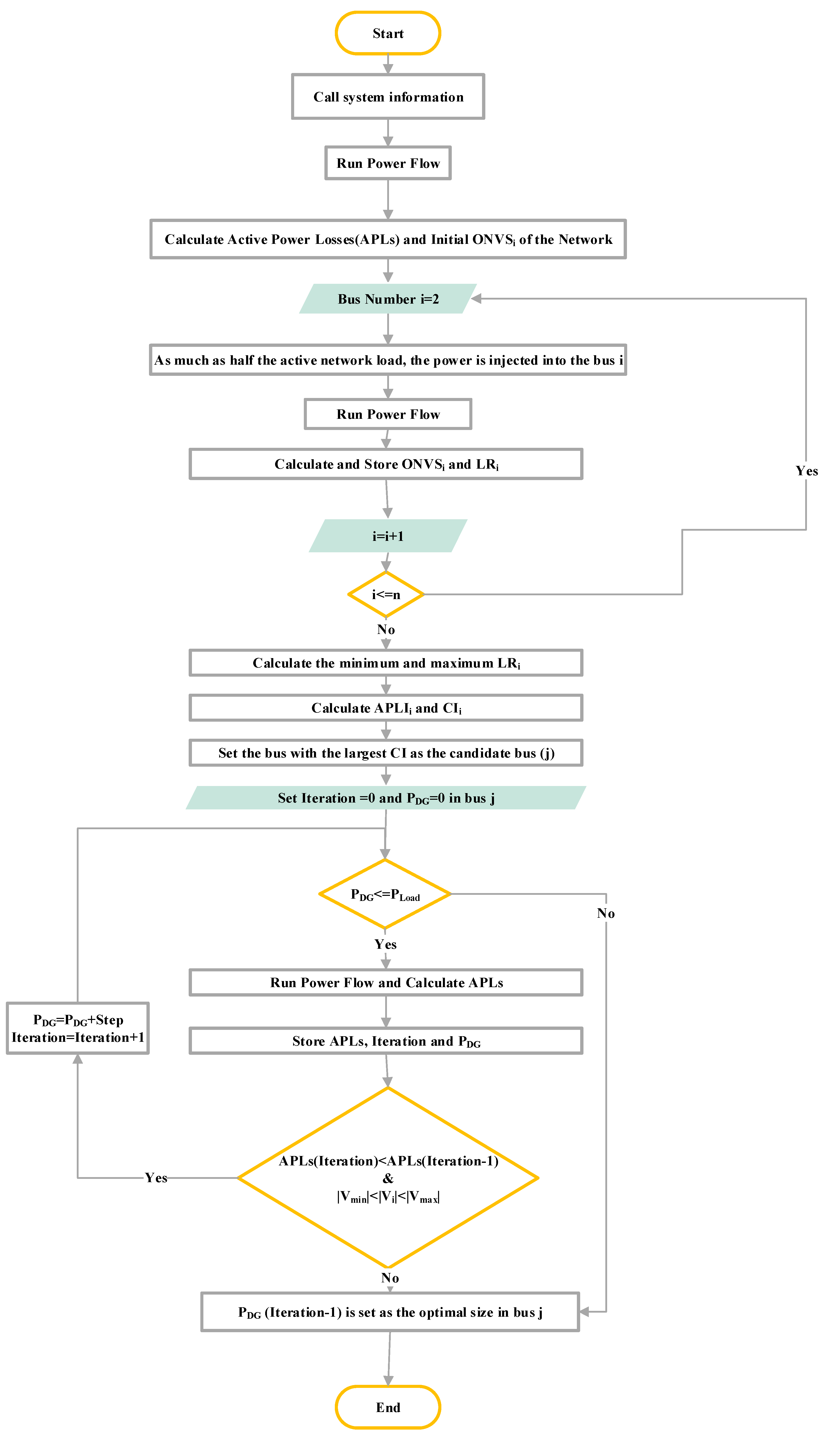
  • Run power flow and calculate initial active power losses.
  • Inject active power equal to half the active power of the entire network to all buses, except the slack bus.
  • Run power flow and calculate active power losses.
  • Calculate the difference between initial active losses and active losses after DG installation.
  • Calculate the maximum and minimum difference between active losses.
  • Calculate the CI index for all buses except the slack bus.
  • The bus with the highest CI value is selected as the candidate bus for DG installation.

2.2. Optimal DG Size

The amount of DG active power varies from 0–100% of total active power by distinguishing the optimal DG venue. Constraints (22) and (23) should be observed when resizing DG. By selecting the optimal DG size, total active power losses and network stability levels decrease and increase, respectively. The relationship between DG size and active network losses follows the parabolic curve; it first decreases and then increases, so the optimal size of DG depends on how much the active power increases at each stage. In this paper, the rate of active power increase at each stage is 1% of the total active power. Optimal DG size is determined by observing the following constraints:
  • Power balance constraint
    P s u b s t a t i o n + P D G = P l o a d + P l o s s
    Q s u b s t a t i o n + Q D G = Q l o a d + Q l o s s
  • Voltage constraint
    | V min | | V i | | V max |
  • DG size constraint
    { P D G P l o a d Q D G Q l o a d

2.3. The Proposed Algorithm

For the studied radial distribution network, active power is calculated for all buses, except the slack bus and the CI value for each bus. The bus with the highest CI value is selected as a candidate bus for DG installation. According to Section 2.2, the search algorithm for determining the optimal DG size in the candidate bus is performed based on the minimum amount of active power losses and compliance with limitations (22) and (23). The proposed scheme’s flowchart for defining the DG’s optimal location and size is shown in Figure 2.

2.4. Energy Losses and DG Cost

For both energy losses and operating costs of DG, we have:
  • Cost of energy losses: annual energy loss cost is obtained by (28):
    C o s t = T A P L × E P × T E P = EnergyPrice   ( $ / Kwh ) T = Period   of   Time   ( h )
    where T = 8760   h and   E P = 0.05 ( $ / Kwh ) .
  • DG cost function
The specifications of the active power cost function for the DG used are shown in (25) [27]:
C ( P D G ) = α P D G 2 + β P D G + ω
where   α = 0 , β = 15 , and   ω = 0.002 .
The specifications of the reactive power cost function for DG are as follows [28]:
C ( Q D G ) = α Q D G 2 + β Q D G + ω
where the coefficients of the cost function depend on the PF and are as follows:
α = α sin 2 ( θ ) ,   β = β sin ( θ ) ,   ω = ω ,   θ = cos ( P F ) 1

3. Results and Discussion

The authors of the paper have considered two RDTSs, including 12 and 33 buses, to implement the proposed method. Based on the proposed CI method, DGs were studied in networks to increase the voltage stability margin and reduce power losses. The output results were calculated using the presented algorithm, in which the results were also compared with CPLS, VSI, and IV methods. The results were obtained for unity and 0.9 lagging power factor, with the apparent power and base voltage of 100 MV and 12.66 kV. Note that Y = 0 in the distribution network because of the low length of the lines. It should be noted that in this paper, the problem under study was examined over a period of one year.

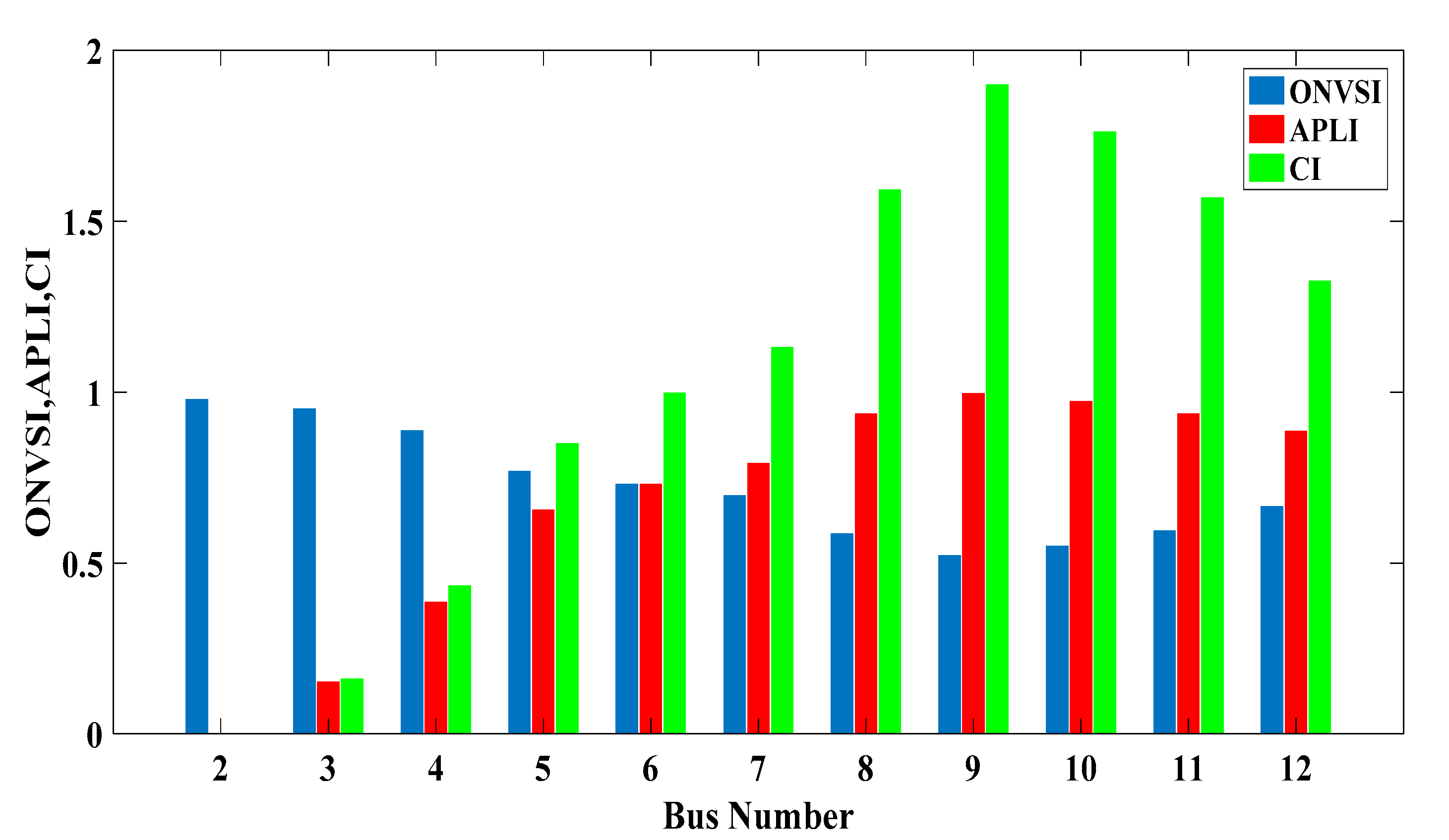
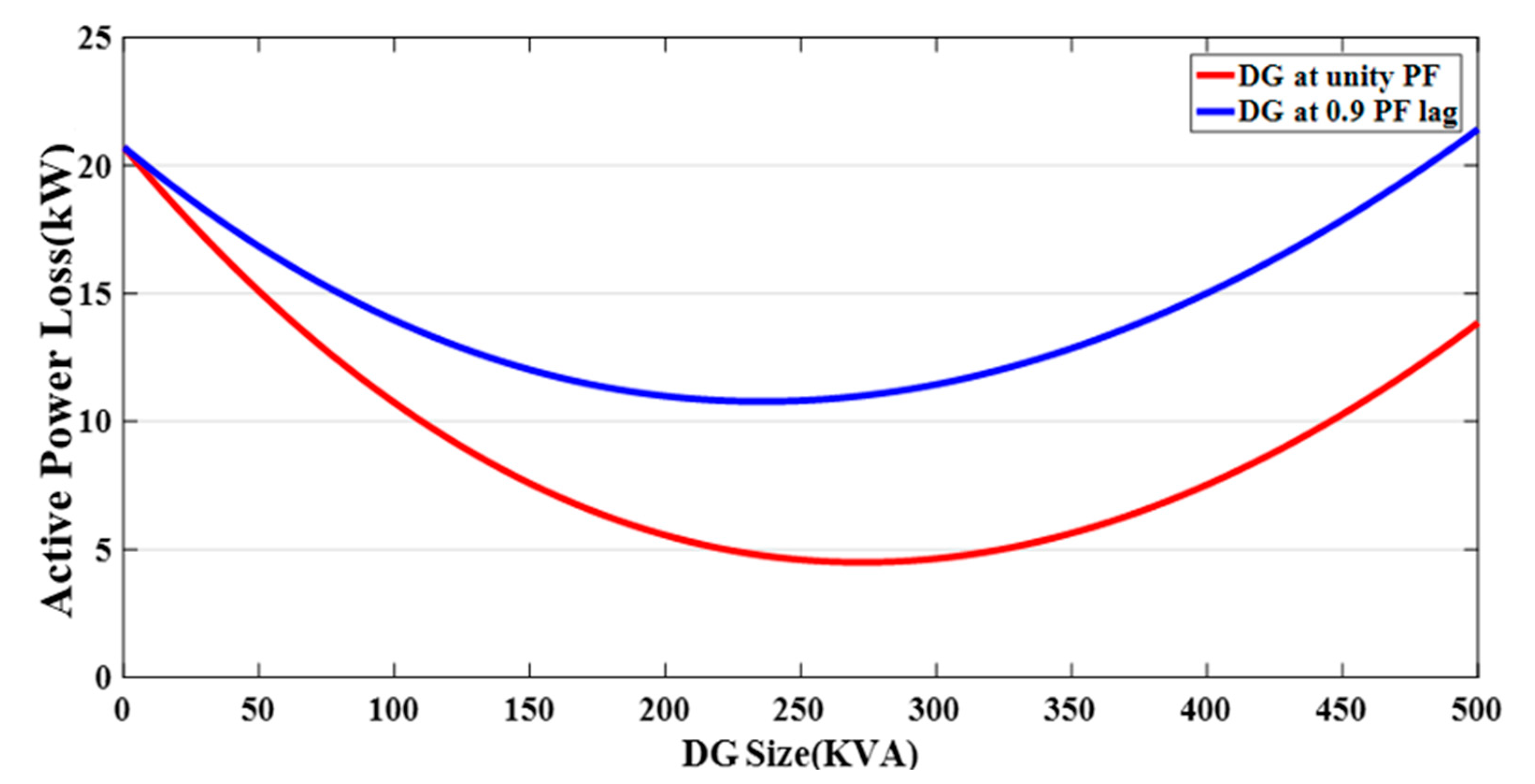
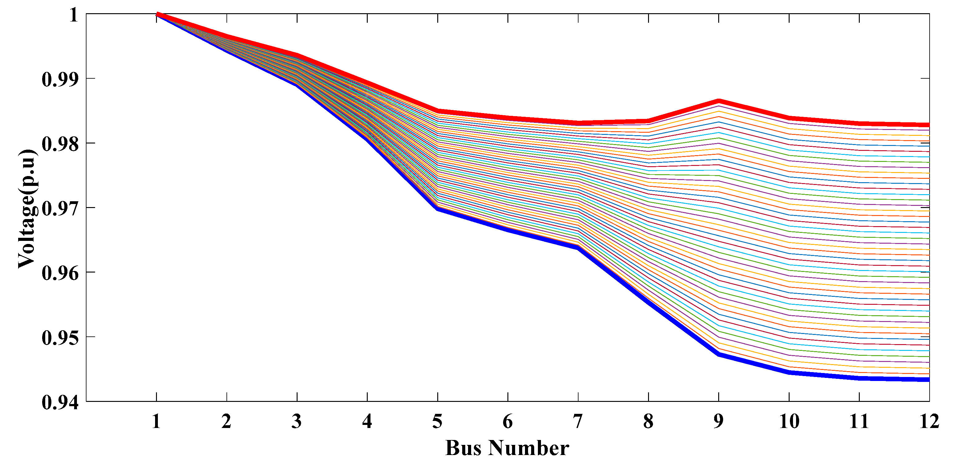
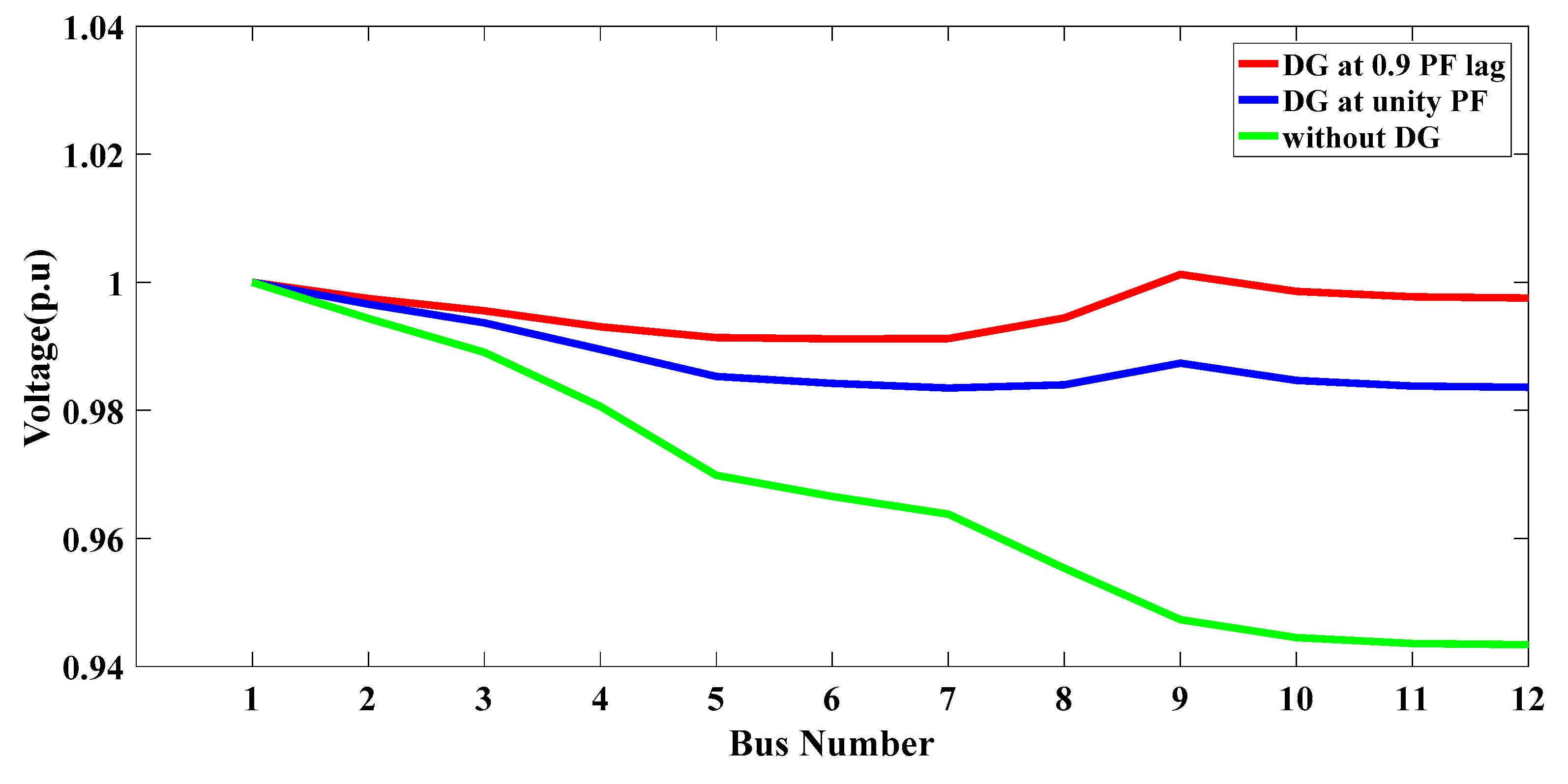
3.1. Results of the IEEE 12-Bus RDTS Test System Based on the Proposed CI Method

For the IEEE 12-bus radial distribution test system, the losses of active and reactive power in DG mode were 207,136 and 80,411 kW, respectively. In this case, the power received from the upstream network was 4,553,366 and 4,130,411 kW. According to the proposed algorithm, APLI, ONVSI, and CI were obtained first to select the candidate points for DG installation. Figure 3 shows the values of these indicators for different buses. An examination of Figure 3 shows that Bus 9 has the lowest ONVSI value, the highest APLI value, and the highest CI value. Therefore, Bus 9 was the most suitable in terms of voltage stability levels and active network losses for DG installation. By placing DG in Bus 9 and injecting active power into the network with a step of 1% of total active load, the changes in active power losses to the DG capacity ratio were obtained. The changes in active power losses are shown in Figure 4 by changing the DG size for a unit power factor and 0.9 lagging. The optimal DG size for the unit power factor and 0.9 lagging is 235.3 kW and 302.33 kVA, respectively. In this case, the minimum active network losses for the unity power factor is 10.7744 kW, and the power factor of which is 0.9 lagging, 4.4929 kW. By installing DG with a unity power factor and 0.9 lagging, respectively, the active and reactive power received from the upstream network is reduced to 210.0974 and 409.1256 kW as well as 167.396 and 274.8582 kW. To observe the effect of DG injection power in the network on bus voltage, a bus voltage profile for DG installation, with the unit power factor, variable capacity between 0 and 235 kV, and a 5 kV step, is shown in Figure 5. As DG injection capacity increases to 235 kW, the voltage profile improves so that the best voltage profile in Figure 5 is for the highest DG capacity, in this case, 235 kW.
The 12-bus voltage profile is shown in DG-installed mode and DG with a unity power factor and 0.9 lagging in Figure 6. For DG with a power factor of 0.9 lagging, the voltage profile phase is more desirable than with the unit power factor. The minimum grid voltage in the two modes with and without DG, with unit power factor and 0.9 phases, are 0.9434, 0.9835, and 0.9912 p.u., respectively. The ONVSI, which was introduced as a voltage level indicator, changed from 1 to 0.5422 and 0.2718 with the installation of DG with unit and 0.9 lagging power factors, which indicates an increase in the voltage stability level.
To further examine the effect of DG installation on increasing network voltage stability levels, the P-V diagram for Bus 9 in Figure 7 was plotted. With DG installation, network load and network voltage stability margins are significantly increased. Installing DG with a 0.9 lagging pf has a more remarkable impact on the level of network voltage stability, which shows the importance of reactive power and attention to power factor optimization.
By installing DG, the studied network becomes an active network. In fact, by installing DG, the active and reactive power passing through the lines is reduced, increasing voltage stability and reducing active and reactive network losses. Reducing losses decreases the cost of annual system active power losses so that the cost of annual energy losses by installing DG with a unity power factor and 0.9 lagging rises from USD 9072.6 to USD 4719.2 and USD 1967.2. By comparing the yearly cost of energy losses before and after installing DG, it is be found that installing DG with a unity power factor and 0.9 lagging saves USD 4353.4 and USD 7105.4 in distribution network costs, respectively. A summary of the DG simulation results is shown in Table 1, with the installation of DG for the IEEE 12-bus RDTS. For unit power factor and a power factor of 0.9-lag, the minimum voltage increases by 4.2% and 5%, respectively. Additionally, the annual cost of energy losses is reduced by 47.95% and 78.32%, respectively.

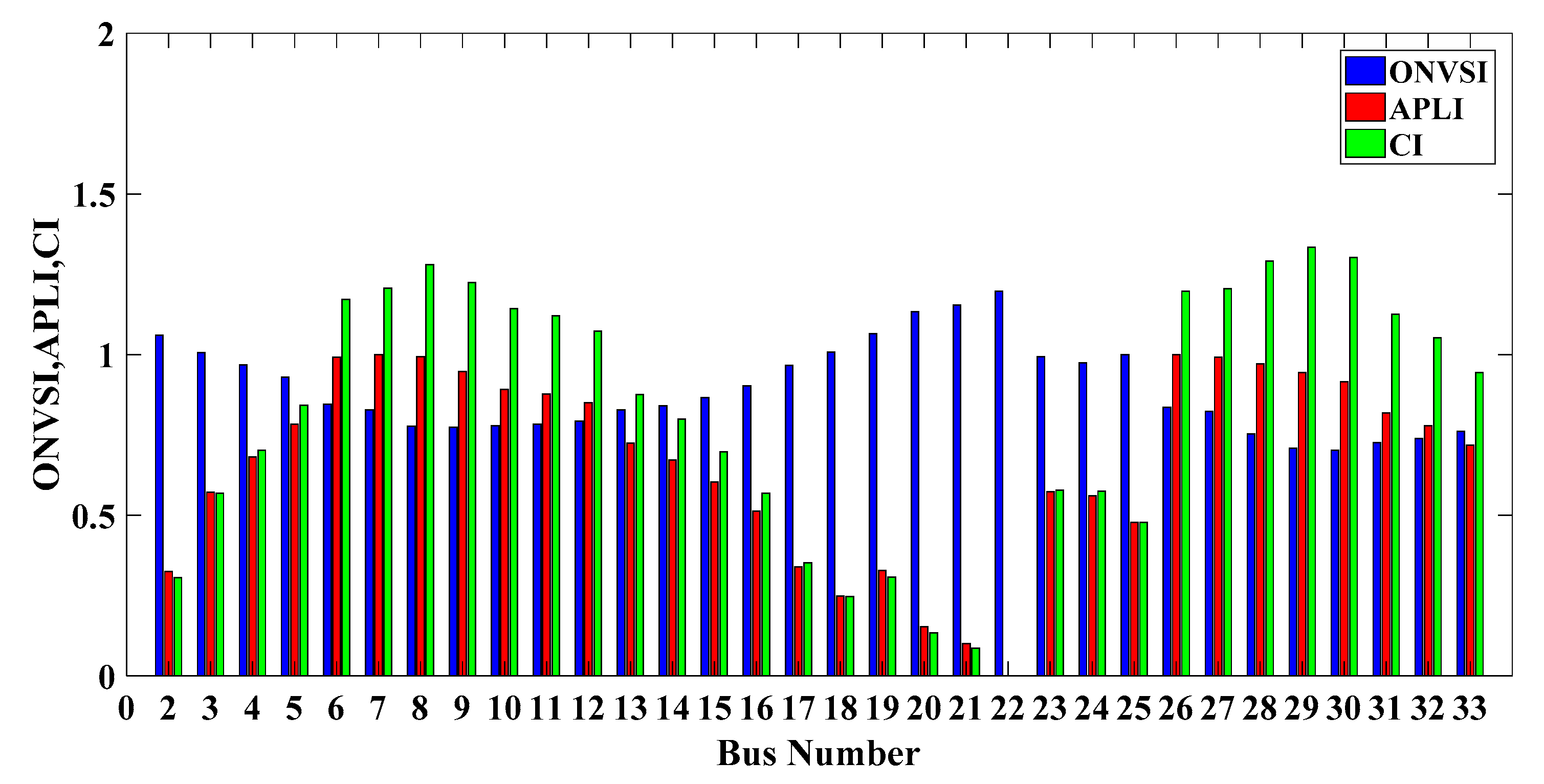
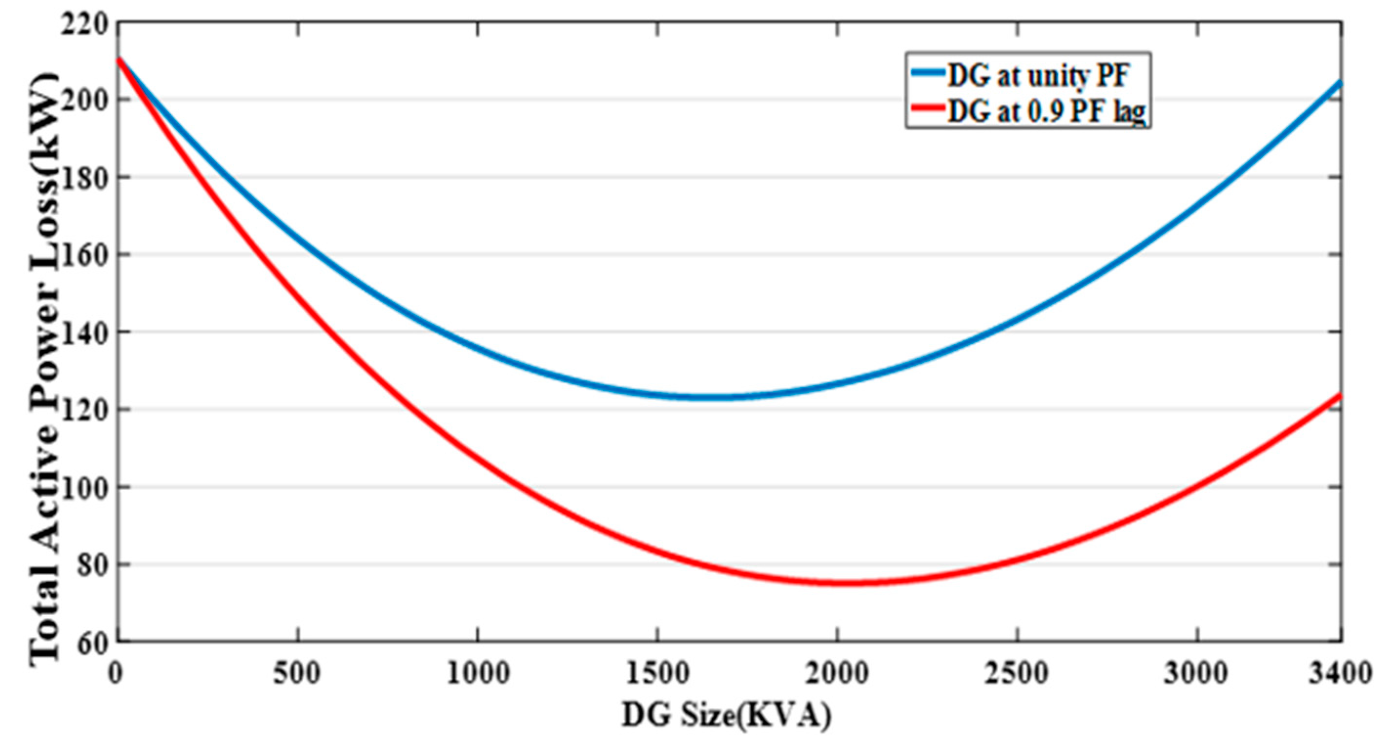
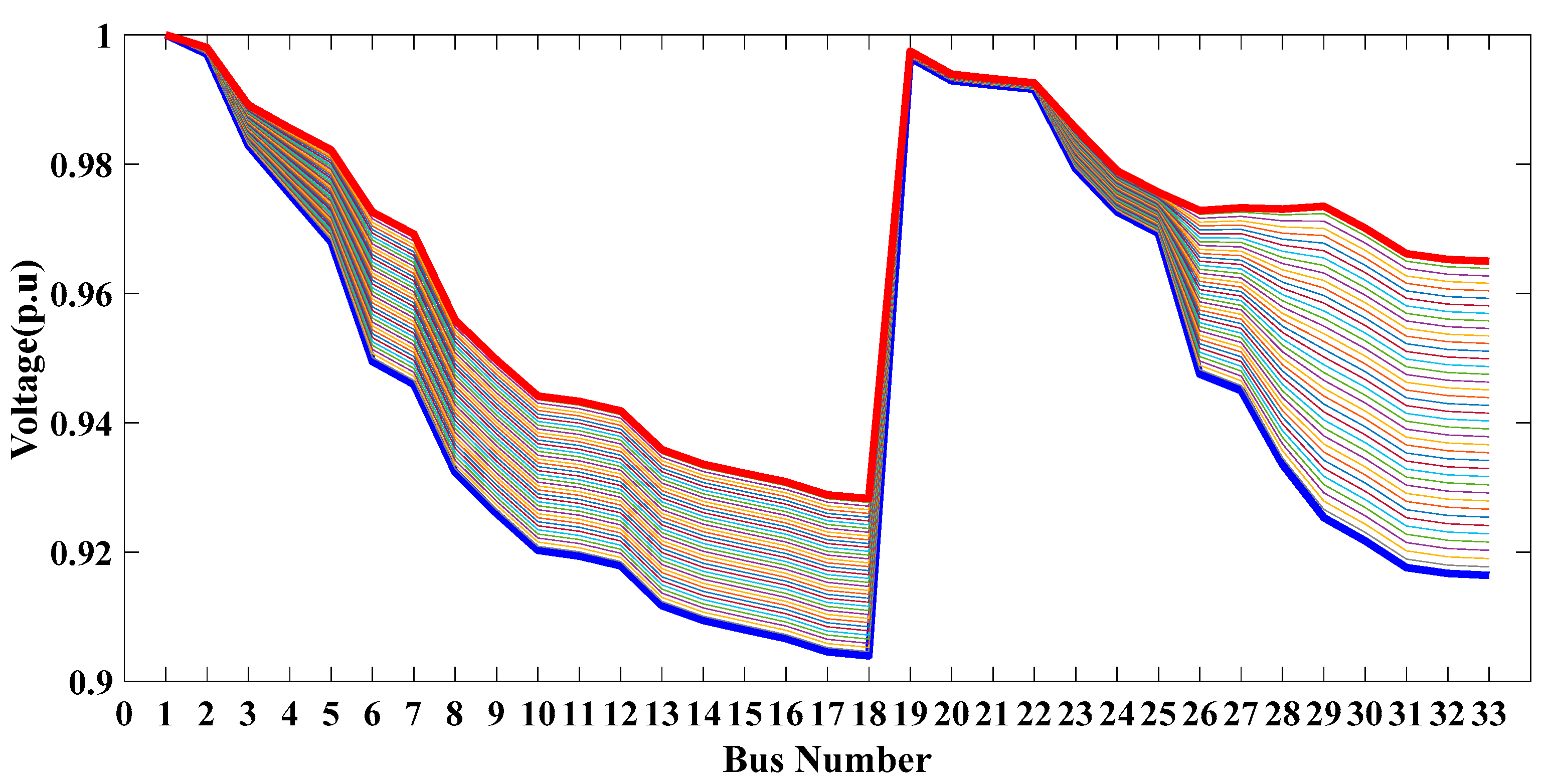
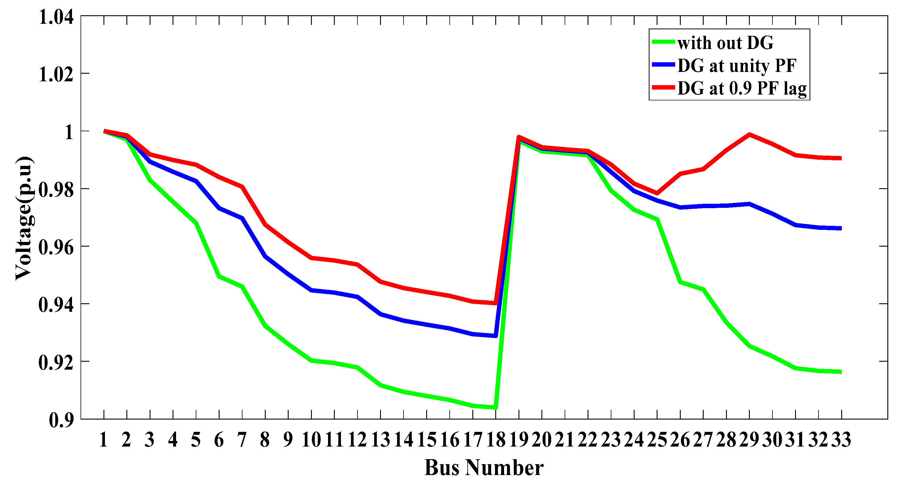
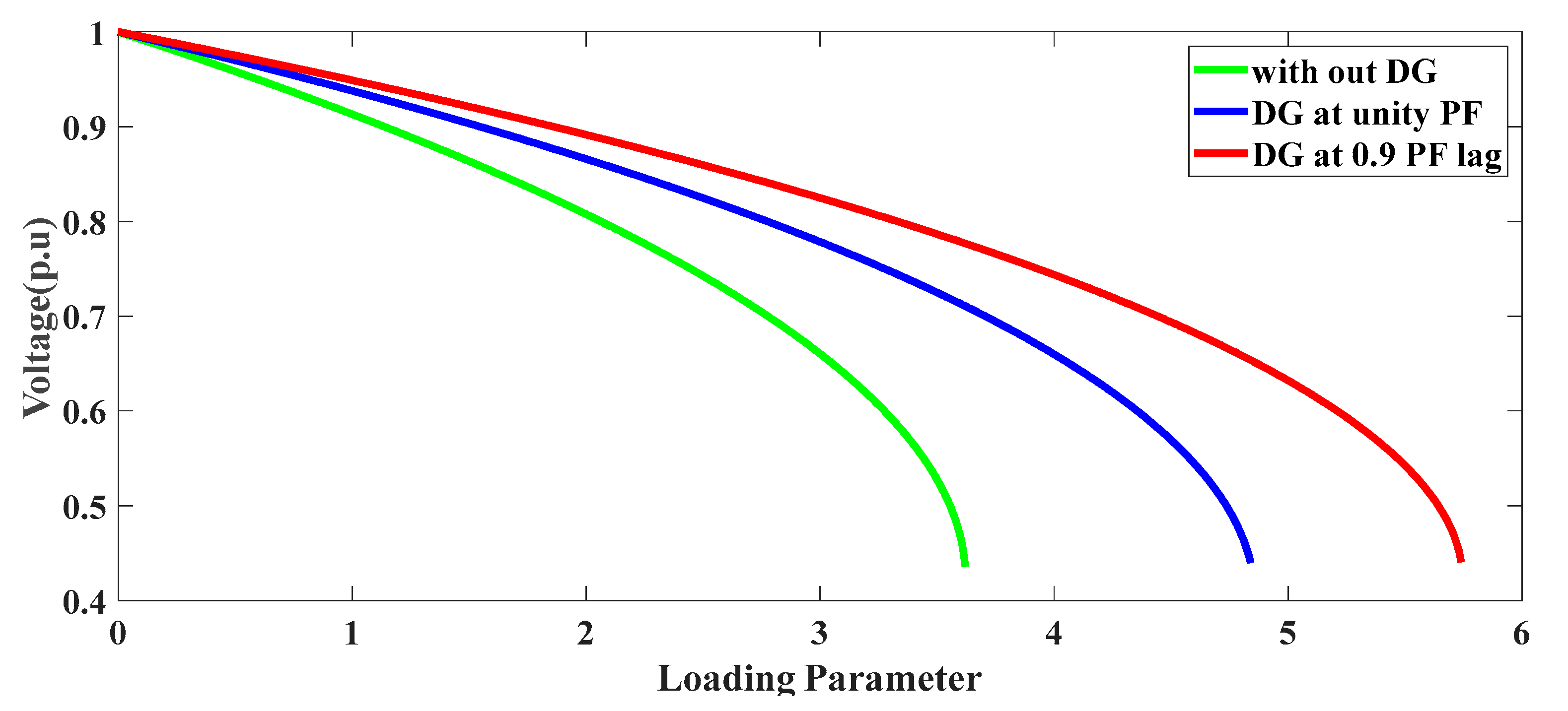
3.2. Results of the IEEE 33-Bus RDTS Based on the Proposed CI Method

In the IEEE 33-bus RDTS test system without DG implementation, the active and reactive power losses are 210.58 and 142.99 kW, respectively. Additionally, in this case, the amount of power received from the upstream network is 3922.2 and 2442.99 kW. Figure 8 shows the value of ONVSI, APLI, and CI for the 33-bus network. Bus 29 is defined as the nominated bus for DG installation because it has the highest CI value. A study of ONVSI for Bus 29 shows that this bus has the lowest ONVSI value after Bus 30. Additionally, in terms of APLI, this bus is one of the most suitable buses for installing DG. After determining Bus 29 as the candidate for DG installation, the next step is to determine the appropriate DG size to reduce energy loss costs. By injecting active power into Bus 29 with a 1% step of the network’s total active power, changes in active losses relative to the DG size are obtained with a unit power factor and 0.9 lagging. Figure 9 shows the network’s active loss changes to DG size. The optimal DG size for the unity power factor is 1646.1 kW, and for the 0.9 lagging pf, 2028 kVA. The total active network losses for DG with a unit power factor and 0.9 lagging are 1,229,849 and 75,026 kW. The active and reactive power received from the upstream network for DG with a unit power factor are 2190.1 and 2388.8 kW, and for DG with a power factor of 0.9 lagging, 1963.2 and 1474.8 kW. As shown in the previous section, the effect of DG resizing on the bus voltage profile of the IEEE 33-bus RDTS system, the voltage profile of different buses for DG installation with a unit power factor and DG resizing from 0 to 1640 kV, with 40 kW step, is depicted in Figure 10. The best voltage profile is for injecting an active power of 1640 kW.
The voltage profile of the IEEE 33-bus RDTS is shown for the two modes, with and without DGs, in Figure 11. In this case, the installation of DG with a unit power factor and 0.9 lagging causes the minimum network voltage to increase from 0.9039 to 0.9288 and 0.9402 p.u. In this paper, ONVSI is defined as an indicator for assessing the level of network voltage stability. The installation of DG with unity and 0.9 lagging pfs will cause the ONVSI value to increase from 1 to 0.7094 and 0.7153, increasing the network voltage stability margin. To examine the effect of DG’s presence on increasing the voltage stability margin and network voltage stability level, the P-V diagram for Bus 18, which has the lowest voltage among the various grid buses, is shown in Figure 12. Studying Figure 12 shows the effect of reactive power on increasing network load and voltage stability margins. These results highlight the importance of optimizing the DG power factor.
Another issue in the discussion of DG optimization is the reduction of network energy losses costs. With optimal DG deployment, the active and reactive power in the transmission network lines changes, and the cost of losses is reduced. With the implementation of DG with a unit power factor and 0.9 lagging, the annual cost of casualties drops from USD 92,234 to USD 53,867 and USD 32,861. In general, with the installation of DG, USD 38,367 and USD 59,373 of energy savings are saved annually. Table 2 summarizes the results of this section for the 33-bus RDTS. For a unit power factor and a power factor of 0.9-lag, the minimum voltage increases by 2.6% and 4%, respectively. Additionally, the annual cost of energy losses is reduced by 41.6% and 64.37%, respectively.

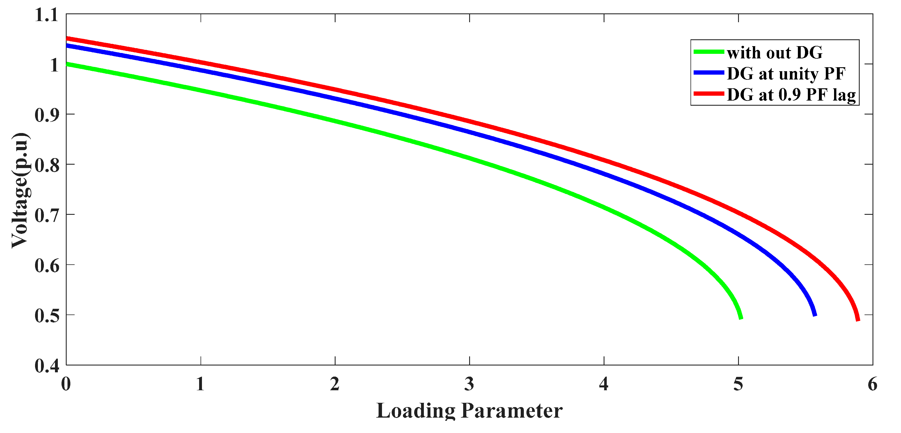
3.3. Optimal Power Factor (OPF)

In this section, the effect of OPF [2] on reducing network losses is investigated. In power systems, to minimize energy losses costs, the DG power factor must be equal to the load power factor:
P F D G = P F l o a d = P l o a d P l o a d 2 + Q l o a d 2
In Section 3.1 and Section 3.2, the power factor value for DG 0.9 was assumed to be lagging, and the losses of Networks 12 and 33 of the bus, as well as the resulting costs, were obtained. In this section, with the help of Equation (27), the OPF for DG is obtained, and the results are compared with the power factor of 0.9 lagging. For the 12-bus and 33-bus networks, the OPF is 0.7319 and 0.85 lagging. Table 3 and Table 4 show the comparison of the results for the optimal and unity pfs. An examination of the results shows a decline in the cost of energy losses with an OPF.

3.4. Comparing the Results with Other Available Methods

This section compares the fruitfulness of the considered algorithm in selecting the optimal location and size of the DG as well as improving the voltage profile and reducing the cost of energy losses. The results for the 12-bus and 33-bus RDTSs with a DG presence, with a unity power factor and 0.9 lagging, are shown in Table 5 and Table 6, respectively. Examining the results shows the proposed algorithm’s proper performance in selecting the optimal location and determining the DG size.
The comparison shows that for the 12-bus RDTS, the four methods examined have provided similar results, which could confirm the presented method’s performance. In the 33-bus RDTS, the considered method performs better than the other methods in reducing losses. In fact, by defining the indices used in the proposed algorithm and using the CI index, the optimal location has been selected appropriately and has reduced network losses.

4. Conclusions

In the presented work, a new CI analytical method for specifying the optimal DG location is presented. The voltage stability index is obtained from a mathematical point of view using the voltage collapse feature, which is of great importance. Using CI to determine the optimal DG location reduces active power losses and improves the voltage profile and stability margin. CI index with sensitivity analysis is effective in improving the voltage profile and reducing the distribution network’s active power losses, which determines the optimal location for DG installation. Then, the optimal size of DG is determined with the aim of active power loss reduction by a search algorithm. Determination of the optimal location and size of DG for three types of DG with unit PF, 0.9 PF lag, and OPF was done. The proposed algorithm was tested on the 12-bus and 33-bus IEEE RDTSs, and the results were analyzed. For IEEE 12- and 33-bus networks, the optimal DG installation location was obtained as Buses 9 and 29, respectively. Additionally, the optimal DG size for these networks with a power factor of 0.9-lag was 314.38 and 2028 kVAr, respectively. The use of the considered algorithm to define the suitable location and size of DG improved the voltage profile and stability margin and reduced active power losses and the resulting costs. Finally, the presented algorithm was compared and validated with IV, VSI, and CPLS methods. Comparing the results shows the effectiveness of the proposed method in reducing active power losses and the resulting costs, as well as improving the network voltage profile. The annual cost of losses for IEEE 12- and 33-bus networks decreased by 78.23% and 64.37%, respectively, which is significant.

Author Contributions

Conceptualization, S.A. and M.M.A.; software, S.A.; validation, A.M., M.T.A. and M.N.H.; formal analysis, M.M.A.; writing—original draft preparation, M.M.A.; writing—review and editing, M.N.H., A.M. and M.T.A., visualization, S.A.; supervision, A.M., M.N.H. and M.T.A.; project administration, M.T.A. All authors have read and agreed to the published version of the manuscript.

Funding

This research received no external funding.

Institutional Review Board Statement

Not applicable.

Informed Consent Statement

Informed consent was obtained from all subjects involved in the study.

Data Availability Statement

Data is generated during the study.

Conflicts of Interest

The authors declare no conflict of interest.

Nomenclature

V S Voltage at bus S
V R Voltage at bus R
δ Phase angle difference between S and R buses
I S Current sent from bus S
I R Current received in bus R
A , B , C , D Line parameters
R Line e resistance
X Line reactance
Z Line impedance
Y Line charging
P R Active power received in bus R
Q R Reactive power received in bus R
j Number of lines
i Bus number

References

  1. Al Abri, R.S.; El-Saadany, E.F.; Atwa, Y.M. Optimal placement and sizing method to improve the voltage stability margin in a distribution system using distributed generation. IEEE Trans. Power Syst. 2012, 28, 326–334. [Google Scholar] [CrossRef]
  2. Hung, D.Q.; Mithulananthan, N. Multiple distributed generator placement in primary distribution networks for loss reduction. IEEE Trans. Ind. Electron. 2011, 60, 1700–1708. [Google Scholar] [CrossRef]
  3. Celli, G.; Pilo, F. Optimal distributed generation allocation in MV distribution networks. In PICA 2001, Innovative Computing for Power-Electric Energy Meets the Market, Proceedings of the 22nd IEEE Power Engineering Society, International Conference on Power Industry Computer Applications, 20–24 May 2001, Sydney, Australia; (Cat. No. 01CH37195); IEEE: Piscataway, NJ, USA, 2001. [Google Scholar]
  4. Prakash, D.; Lakshminarayana, C. Multiple DG placements in radial distribution system for multi objectives using Whale Optimization Algorithm. Alex. Eng. J. 2018, 57, 2797–2806. [Google Scholar] [CrossRef]
  5. Kayal, P.; Chanda, C.K. Placement of wind and solar based DGs in distribution system for power loss minimization and voltage stability improvement. Int. J. Electr. Power Energy Syst. 2013, 53, 795–809. [Google Scholar] [CrossRef]
  6. Murty, V.V.S.N.; Kumar, A. Optimal placement of DG in radial distribution systems based on new voltage stability index under load growth. Int. J. Electr. Power Energy Syst. 2015, 69, 246–256. [Google Scholar] [CrossRef]
  7. Hedayati, H.; Nabaviniaki, S.A.; Akbarimajd, A. A method for placement of DG units in distribution networks. IEEE Trans. Power Deliv. 2008, 23, 1620–1628. [Google Scholar] [CrossRef]
  8. Ettehadi, M.; Ghasemi, H.; Vaez-Zadeh, S. Voltage stability-based DG placement in distribution networks. IEEE Trans. Power Deliv. 2012, 28, 171–178. [Google Scholar] [CrossRef]
  9. Esmaili, M.; Firozjaee, E.C.; Shayanfar, H.A. Optimal placement of distributed generations considering voltage stability and power losses with observing voltage-related constraints. Appl. Energy 2014, 113, 1252–1260. [Google Scholar] [CrossRef]
  10. Aman, M.; Jasmon, G.; Mokhlis, H.; Bakar, A. Optimal placement and sizing of a DG based on a new power stability index and line losses. Int. J. Electr. Power Energy Syst. 2012, 43, 1296–1304. [Google Scholar] [CrossRef]
  11. Memarzadeh, G.; Keynia, F. A new index-based method for optimal DG placement in distribution networks. Eng. Rep. 2020, 2, e12243. [Google Scholar] [CrossRef]
  12. Prakash, D.B.; Lakshminarayana, C. Multiple DG placements in distribution system for power loss reduction using PSO Algorithm. Procedia Technol. 2016, 25, 785–792. [Google Scholar] [CrossRef] [Green Version]
  13. Prabha, D.R.; Jayabarathi, T. Optimal placement and sizing of multiple distributed generating units in distribution networks by invasive weed optimization algorithm. Ain Shams Eng. J. 2016, 7, 683–694. [Google Scholar] [CrossRef] [Green Version]
  14. Taheri, S.I.; Salles, M.B.C. A New Modification for TLBO Algorithm to Placement of Distributed Generation. In Proceedings of the 2019 International Conference on Clean Electrical Power (ICCEP), Otranto, Italy, 2–4 July 2019. [Google Scholar]
  15. Ganguly, S.; Samajpati, D. Distributed generation allocation on radial distribution networks under uncertainties of load and generation using genetic algorithm. IEEE Trans. Sustain. Energy 2015, 6, 688–697. [Google Scholar] [CrossRef]
  16. Gandomkar, M.; Vakilian, M.; Ehsan, M. A combination of genetic algorithm and simulated annealing for optimal DG allocation in distribution networks. In Proceedings of the Canadian Conference on Electrical and Computer Engineering, Saskatoon, SK, Canada, 1–4 May 2005. [Google Scholar]
  17. Kefayat, M.; Ara, A.L.; Niaki, S.N. A hybrid of ant colony optimization and artificial bee colony algorithm for probabilistic optimal placement and sizing of distributed energy resources. Energy Convers. Manag. 2015, 92, 149–161. [Google Scholar] [CrossRef]
  18. Kowsalya, M. Optimal size and siting of multiple distributed generators in distribution system using bacterial foraging optimization. Swarm Evol. Comput. 2014, 15, 58–65. [Google Scholar]
  19. Nazari-Heris, M.; Madadi, S.; Hajiabbas, M.P.; Mohammadi-Ivatloo, B. Optimal distributed generation allocation using quantum inspired particle swarm optimization. In Quantum Computing: An Environment for Intelligent Large Scale Real Application; Springer: Cham, Switzerland, 2018; pp. 419–432. [Google Scholar]
  20. Pesaran, H.A.M.; Nazari-Heris, M.; Mohammadi-Ivatloo, B.; Seyedi, H. A hybrid genetic particle swarm optimization for distributed generation allocation in power distribution networks. Energy 2020, 209, 118218. [Google Scholar] [CrossRef]
  21. Selim, A.; Kamel, S.; Alghamdi, A.S.; Jurado, F. Optimal Placement of DGs in Distribution System Using an Improved Harris Hawks Optimizer Based on Single-and Multi-Objective Approaches. IEEE Access 2020, 8, 52815–52829. [Google Scholar] [CrossRef]
  22. Suresh, M.C.V.; Edward, J.B. A hybrid algorithm based optimal placement of DG units for loss reduction in the distribution system. Appl. Soft Comput. 2020, 91, 106191. [Google Scholar] [CrossRef]
  23. Elattar, E.E.; Elsayed, S.K. Elsayed. Optimal location and sizing of distributed generators based on renewable energy sources using modified moth flame optimization technique. IEEE Access 2020, 8, 109625–109638. [Google Scholar] [CrossRef]
  24. Das, D.; Nagi, H.S.; Kothari, D.P. Novel method for solving radial distribution networks. IEE Proc.-Gener. Transm. Distrib. 1994, 141, 291–298. [Google Scholar] [CrossRef]
  25. Baran, M.; Wu, F.F. Optimal sizing of capacitors placed on a radial distribution system. IEEE Trans. Power Deliv. 1989, 4, 735–743. [Google Scholar] [CrossRef]
  26. Murthy, V.V.S.N.; Kumar, A. Comparison of optimal DG allocation methods in radial distribution systems based on sensitivity approaches. Int. J. Electr. Power Energy Syst. 2013, 53, 450–467. [Google Scholar] [CrossRef]
  27. Gautam, D.; Mithulananthan, N. Optimal DG placement in deregulated electricity market. Electr. Power Syst. Res. 2007, 77, 1627–1636. [Google Scholar] [CrossRef]
  28. Hasanpour, S.; Ghazi, R.; Javidi, H. A new approach for cost allocation and reactive power pricing in a deregulated environment. Electr. Eng. 2009, 91, 27. [Google Scholar] [CrossRef]
Figure 1. The two-bus system studied for modeling the voltage stability index.
Sustainability 13 10224 g001
Figure 2. Flowchart of the proposed scheme.
Sustainability 13 10224 g002
Figure 3. The values for ONVSI, APLI, and CI for the IEEE 12-bus RDTS.
Sustainability 13 10224 g003
Figure 4. Changes in DG-sized with active power losses in the IEEE 12-bus RDTS.
Sustainability 13 10224 g004
Figure 5. The effect of DG injection power on the voltage profile.
Sustainability 13 10224 g005
Figure 6. The IEEE 12-bus RDTS test system voltage profile.
Sustainability 13 10224 g006
Figure 7. The effect of DG installation on increasing loading capacity and system voltage stability.
Sustainability 13 10224 g007
Figure 8. The amount of ONVSI, APLI, and CI for the IEEE 33-bus RDTS.
Sustainability 13 10224 g008
Figure 9. Changes in DG-sized active power losses in the IEEE 33-bus RDTS.
Sustainability 13 10224 g009
Figure 10. The effect of DG injection power on the voltage profile.
Sustainability 13 10224 g010
Figure 11. The IEEE 33-bus RDTS system voltage profile.
Sustainability 13 10224 g011
Figure 12. The effect of DG installation on increasing load and voltage stability.
Sustainability 13 10224 g012
Table 1. The results of the IEEE 12-bus RDTS.
ItemsBase CaseDG PF
Unit0.9 lag
Location-99
Size (kVA)-235.3314.38
Active power losses (kw)20.713610.77444.4929
Table 2. The results of the IEEE 33-bus RDTS.
ItemsBase CaseDG PF
Unit0.9 lag
Location-2929
Size (kVA)-1646.12028
Active power losses (kw)210.58122.9875.03
Reactive power losses (kVAr)142.9988.8458.88
Minimum bus voltage (p.u)0.90390.92880.9402
Active power from the upstream (kw)3922.22190.11963.1
Reactive power from the upstream (kVAR)442.992388.81474.8
Cost of energy losses ($)92,23453,86732,861
Net savings ($)-38,36759,373
%savings-41.664.37
C(PDG) ($/h)-24.620527.382
C(QDG) ($/h)--5.7838
Table 3. The results of the IEEE 12-bus RDTS for OPF.
ItemsBase CaseDG PF
Unit0.7319 lag
Location-99
Size (kVA)-235.3314.38
Active power losses (kw)20.713610.77443.1577
Reactive power losses (kVAr)8.04114.12561.1093
Minimum bus voltage (p.u)0.94340.98350.9907
Active power from the upstream (kw)455.3366210.0974208.06
Reactive power from the upstream (kVAR)413.0411409.1256191.88
Cost of energy losses ($)9072.64719.21383.1
Net savings ($)-4353.47689.5
%savings-47.9584.76
C(PDG) ($/h)-3.53343.4555
C(QDG) ($/h)--1.602
Table 4. The results of the IEEE 33-bus RDTS for OPF.
ItemsBase CaseDG PF
Unit0.85 lag
Location-2929
Size (kVA)-1646.12097.7
Active power losses (kw)210.58122.9872.56
Reactive power losses (kVAr)142.9988.8455.77
Minimum bus voltage (p.u)0.90390.92880.9417
Active power from the upstream (kw)3922.22190.11954.5
Reactive power from the upstream (kVAR)442.992388.81418
Cost of energy losses ($)92,23453,86731,781
Net savings ($)-38,36760,453
%savings-41.665.54
C(PDG) ($/h)-24.620526.746
C(QDG) ($/h)--8.73
Table 5. Comparing the obtained results for a unity PF (IEEE 12-bus RDTS).
ItemsIV [21]CPLS [21]VSI [24]Proposed Method
Location9999
Size (kVA)232.14231.69235235.3
Active power losses (kw)10.77510.77610.773910.7744
Reactive power losses (kVAr)4.13014.13294.12594.1256
Minimum bus voltage (p.u)0.983120.983070.983490.9835
Table 6. Comparing the results for a 0.9 PF lag (IEEE 33-bus RDTS).
ItemsIV [21]CPLS [21]VSI [24]Proposed Method
Location3083329
Size (kVA)195021001570.82028
Active power losses (kw)78.484.596.675
Reactive power losses (kVAr)58.962.177.2658.88
Minimum bus voltage (p.u)0.93910.95340.93220.9402
Publisher’s Note: MDPI stays neutral with regard to jurisdictional claims in published maps and institutional affiliations.

