The Heavy Burden of “Dependent Children”: An Italian Story

Abstract

This paper analyses multidimensional fuzzy monetary and non-monetary deprivation in households with children by using two different definitions: households with children under 14 years old, and the EU definition of households with dependent children. Eight dimensions of non-monetary deprivation were found using 34 items from the EU-SILC 2016 survey. Dealing with subpopulations, it is essential to compute standard errors for the presented estimators. Thus, a relevant added value of the paper is fuzzy poverty measures and associated standard errors, which were also computed. Moreover, a comparison was made between the measures obtained concerning the two subpopulations across countries. With a focus on Italy, an Italian macro-region is presented.

1. Introduction

Children are more vulnerable to poverty and deprivation and the poverty that they experience can compromise their outcomes in future adult life. In 2018, one out of four children (aged 0–18) in the EU were at risk of poverty or social exclusion. However, as reported by Eurostat [1], child poverty rates vary significantly between member states. In Romania, Bulgaria, Greece, and Italy, one out of three children were found to be at risk of poverty or social exclusion, while in Denmark, the Netherlands, the Czech Republic, and Slovenia, only one out of six children were at risk in 2018. Most of the EU countries stated that the at-risk-of-poverty rate was highest for single persons with dependent children. Regarding Italy, there are several particular points to observe. Italy (with Spain and Greece) reported the highest at-risk-of-poverty or social exclusion rate (nearly 20%) in EU member countries for households with two adults and one dependent, while nearly 40% of households with two adults and three or more dependent children are at risk of poverty (only Bulgaria and Romania report higher figures). It seems that the burden of dependent children weighs more heavily in Italy than in other member states. A consideration that could aid our understanding of this issue is an aspect of Italian culture in which the average age at which children leave home is much higher than what is found in many other European countries. Therefore, children depend on their parents for a long time. Consequently, the first original contribution of this paper consists in carrying out a deeper analysis by considering two different definitions of households with children: the first is households with at least one child aged 0–14 years, and the second consists of households with at least one dependent child. A second original contribution of the paper is the computation of the standard errors for the fuzzy measures, performed from complex sample surveys, such as EU-SILC.

The rest of the paper is organized as follows. Section 2 presents the data used for the analysis and delineates the research methodology. Section 3 presents the findings of the study, while Section 4 reports some final remarks.

2. Data and Methodology

The aims of this section are the following: to introduce the data set used for the analysis and the variables involved, as well as to include relevant information regarding the methodology, the approach, and the operationalization.

2.1. Data

This paper uses the 2016 wave of the European Union Statistics on Income and Living Conditions (EU-SILC). It provides multidimensional microdata on income and living conditions in the European Union. Other than that, the ad hoc modules developed in 2016, “Access to Services”, includes variables concerning access to childcare, home care, training, education, and healthcare.

Access to education and healthcare services is important and closely linked to living conditions for all household members. Education has an important impact on an individual’s income as well as on their knowledge and culture. Better access to healthcare can improve life expectancy in addition to well-being. Access to childcare, too, has an important impact on household income in that the lack of access to childcare affects the work-family balance of women and actually reduces active female participation in the labor market. Moreover, childcare services improve the life chances of all children, especially those who are disadvantaged, by stimulating their learning. Moreover, these services offer children the opportunity to become familiar with those from different backgrounds.

The target variables involved in the analysis relate to different types of units.

Information on social exclusion, housing conditions, and material deprivation is collected mainly at the household level, while labor, education, and health information is collected at the individual level for everyone age 16 and over. Detailed data are collected on income components, primarily on personal income, and then they are aggregated at the household level to construct the household income. The income variables considered in the current analysis are the total disposable household income (HY020) and the total disposable household income before social transfers other than old-age and survivor’s benefits (HY022). Both are adjusted for inflation and converted into the equivalized household income using the so-called modified Organization for Economic Co-operation and Development (OECD) equivalence scale, which weights (Organization for Economic Cooperation and Development, 2009) the first adult by 1.0, the second adult and each subsequent individual aged 14 and over by 0.5, and then 0.3 to each child under 14 years. Regarding the variables collected by the 2016 module on “Access to Services”, the variables chosen for the analysis are those related to affordability of the service, specifically the following: affordability of formal education, affordability of healthcare services, and affordability of childcare services. These variables apply at the household level and refer to the household [2].

Our analysis considers the cross-section sample of households included in the 2016 wave of the EU-SILC. The countries involved in the analysis are as follows: Austria, Belgium, Bulgaria, Switzerland, Cyprus, Czech Republic, Denmark, Estonia, Greece, Spain, France, Hungary, Ireland, Iceland, Italy, Luxembourg, Latvia, Norway, Poland, Portugal, Serbia, Sweden, and Slovakia (Some member states were removed from the analysis because of high missing values in the considered variables, or variables that were not collected at all, or because of problems of sample sizes in households with children). Specifically, we are interested in two sets of households: those with at least one child aged 0–14 years and households with at least one dependent child. A dependent child is any person below 18 years as well as those who are from 18 to 24 years old, living with at least one parent, and who are economically inactive. Using this criterion, the sets of households analyzed consist of 42,817 and 52,871 households, respectively

Table 1. Sample sizes of households with children 0–14 years old and households with dependent children.

	Number of Households (% of Total Households)	Number of Individuals (% of Total Individuals)
Households with children aged 0–14	42,817 (22.6%)	172,478 (37.0%)
Households with dependent children	52,871 (27.9%)	214,549 (46.1%)

.

2.2. Methods

The consensus on the fact that poverty must be seen and measured as a multidimensional phenomenon is also recognized in the 2030 UN Agenda for Sustainable Development, which identifies the reduction of poverty in “all its forms and dimensions” among the objectives to be achieved. The adopted methodology is based on the cross-sectional fuzzy multidimensional measures of deprivation (monetary and non-monetary) that treats poverty as a matter of degree [3]. Defining poverty as a matter of degree has several advantages, as highlighted by [4]. First, non-monetary poverty is subject to forced non-access to various facilities or possessions that determine basic living conditions, or an individual might have access to only some of them. Second, but not less important, the fuzzy approach provides more robust indicators [5], so it is particularly indicated for studying subpopulations or small domains, as in our case, for households with children.

In treating monetary and non-monetary poverty with a fuzzy approach, the fundamental point is the choice of the membership function that quantifies the propensity of each person to poverty. We chose the membership function defined by [6], and further elaborated by [7], which includes the relative poverty measure of the so-called “Totally Fuzzy and Relative” (TFR) function [8]. In this way, two indicators are defined: the Fuzzy Monetary (FM, K = 1) indicator for monetary poverty and the Fuzzy Supplementary (FS, K = 2) indicator for non-monetary poverty. Accordingly, the propensity to poverty and deprivation for any individual, i, is specified through the “Integrated Fuzzy and Relative” (IFR) membership function, defined as:

$${\mu }_{i,K}={{\left(\frac{{\displaystyle \sum _{\gamma =i+1}^n{w}_{\gamma }|X_{\gamma }>X_i}}{{\displaystyle \sum _{\gamma =2}^n{w}_{\gamma }|X_{\gamma }>X_1}}\right)}^{{\alpha }_K-1}\left(\frac{{\displaystyle \sum _{\gamma =i+1}^n{w}_{\gamma }{X}_{\gamma }|X_{\gamma }>X_i}}{{\displaystyle \sum _{\gamma =2}^n{w}_{\gamma }{X}_{\gamma }|X_{\gamma }>X_1}}\right)}_{i=1,\dots , n-1}$$

(1)

where X is the equivalized income in the FM or the overall score in the FS, $w_{\gamma }$ is the sample weight of each statistical unit of rank $\gamma$, and ${\alpha }_K$ are parameters corresponding to monetary and non-monetary aspects of poverty. Each parameter ${\alpha }_K$ is estimated so that the mean of the corresponding membership function is equal to the head count ratio (HCR), officially known as the at-risk-of-poverty rate (ARPR), which is computed on the basis the official poverty line (60% of the median national equivalized income). It is important to note that the two parameters ${\alpha }_K$ have a very precise economic interpretation, that is, the mean of the membership functions are expressible in terms of the generalized Gini measures $G_{{\alpha }_K}$, which is a generalization of the standard Gini coefficient, $\frac{{\alpha }_K+G_{{\alpha }_K}}{{\alpha }_K\left({\alpha }_K+1\right)}=ARPR$ [9]. In other words, such fuzzy poverty measures, intrinsically being highly relative, also constitute a good inequality measure.

Reference [7] also proposed a step-by-step procedure for measuring the FS that can be briefly summarized as follows:

• Identification of items to describe non-monetary poverty and their transformation into the range [0, 1];
• Development of exploratory and confirmatory factor analysis to identify the hidden dimensions of poverty;
• Construction of the weights to be assigned within each dimension, based on the dispersion of the item and the correlation with other items belonging to the same dimension;
• Computation of the score within each dimension as a weighted mean of the items in the dimension, and finally, computation of the overall score as a simple average of the dimension scores.

In the present study, 34 items were identified from the EU-SILC 2016 database to investigate non-monetary deprivation within households with children who are under 14 year old or households with dependent children. After their transformation into the range [0, 1], the exploratory factor analysis enabled us to identify eight hidden dimensions of multidimensional non-monetary poverty. The dimensions identified are reported in

Table 2. Details on the dimensions of non-monetary poverty.

1. Basic Lifestyle	2. Consumer Durables	3. Housing Amenities	4. Financial Situation	5. Environment	6. Work and Education	7. Service Affordability	8. Health Related
Meals with meat, fish, or chicken;	Car;	Bath or Shower;	Inability to cope with unexpected expenses;	Crime, violence, vandalism;	Early school leavers;	Affordability of childcare services;	General health;
Household adequately warm;	PC;	Indoor flushing toilet;	Arrears on mortgage or rent payments;	Pollution;	Low education;	Affordability of formal education;	Chronic illness;
Holiday away from home;	Telephone;	Leaking roof and damp;	Arrears on utility bills;	Noise.	Worklessness;	Affordability of healthcare services.	Mobility restriction;
Ability to make ends meet	Washing Machine;	Rooms too dark;	Arrears on hire purchase instalments;		Duration of unemployment.		Unmet need for medical exam;
	TV	Overcrowded house (NEW).	Financial burden of total housing cost (NEW).				Unmet need for dental exam.

.

Most of the 34 items have already been used in the literature on multidimensional non-monetary poverty, and their strength in describing it have been proved (see, for example [7]). However, in this study, we decided to add a new dimension on service affordability, using three items from the EU-SILC ad hoc module 2016, in addition to one item from the dimension on housing amenities (overcrowd house), and one from the dimension on financial situation (financial burden of total housing costs).

The construct validity was validated through a confirmatory factor analysis that confirmed the subsample of households with at least one child aged 0–14 years and for households with at least one dependent child. In

Table 3. Confirmatory factor: goodness of fit.

	Households with Children Aged 0–14	Households with Dependent Children
Goodness of fit (GFI) a	0.928	0.929
Adjusted GFI b	0.913	0.914
Parsimonious GFI c	0.811	0.811
Std. Root Mean Square Residual d	0.056	0.058
RMSEA e	0.049	0.049

^a Based on the ratio of the sum of squared discrepancies to the observed variances, which ranges in [0, 1], with higher values indicating a good fit. ^b The GFI adjusted for degrees of freedom of the model, that is, the number of the fixed parameters. It can be interpreted in the same way as the previous one. ^c Adjusts GFI for the number of estimated parameters in the model and the number of data points. ^d The fit is considered really good if RMR is equal or below 0.06. ^e The Root Mean Squared Error of Approximation (RMSEA) is based on the analysis of residuals, with small values indicating a good fit (<0.05 good fit).

, the main goodness-of-fit indexes are reported, which are very similar for both samples and all of them are very good, again highlighting the goodness of the chosen items and dimensions for non-monetary poverty.

Then, the FS weights for each dimension and the overall weights were computed. Fuzzy monetary poverty was implemented by using three different incomes, namely, household equivalized income (HX090), household disposable income (HY020), and household disposable income before social transfers (HY022). This was done to compare the impact of different definitions of poverty, but most of all, to evaluate the impact of social transfers.

3. Results

To compare the deprivation status for households with at least one child aged 0–14 years and for households with at least one dependent child, the analyses were conducted separately by considering the two different sets of households. The results derive from the methodology explained in Section 2 and refer to the monetary and non-monetary dimensions of poverty for each EU country involved in the analysis.

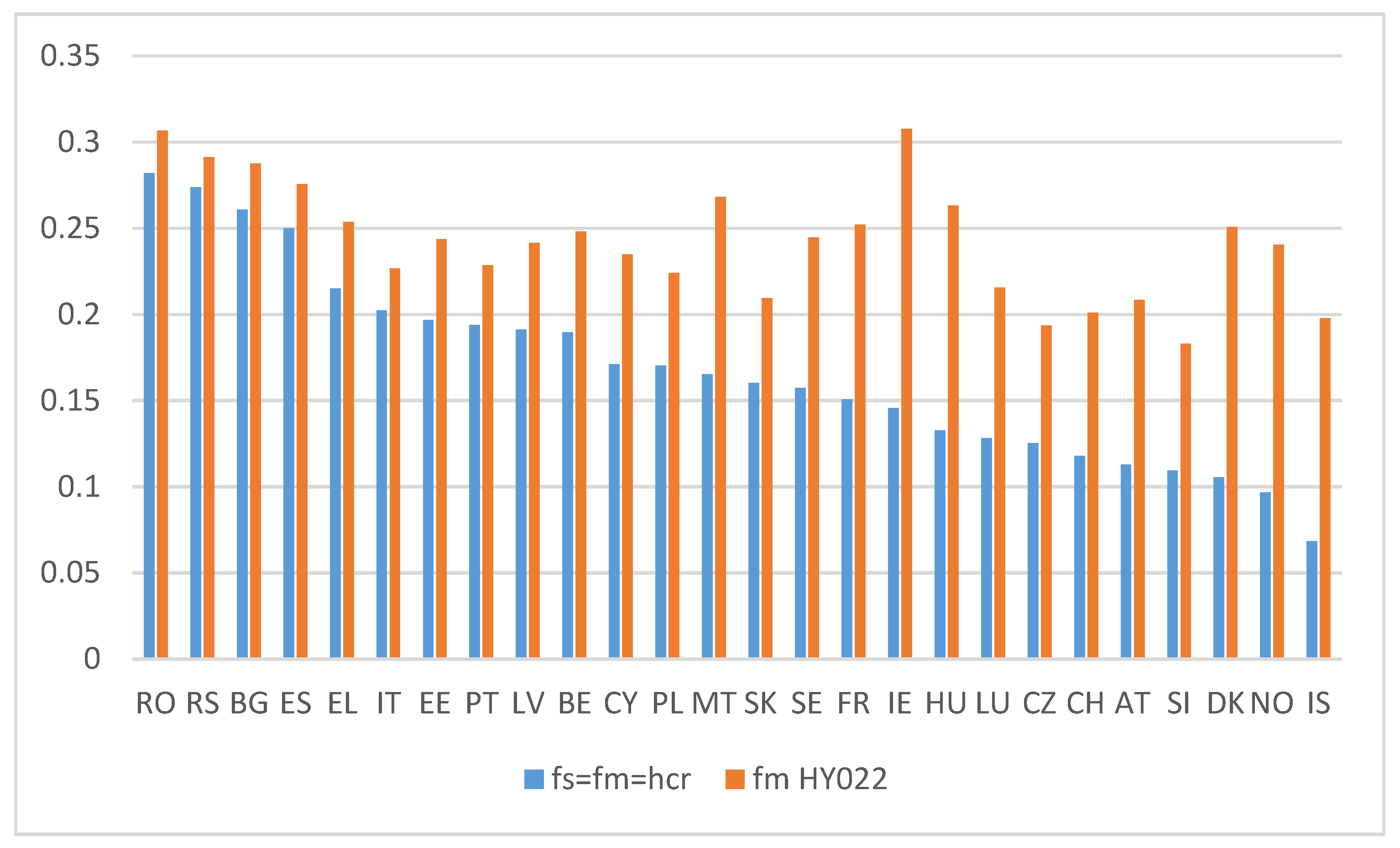
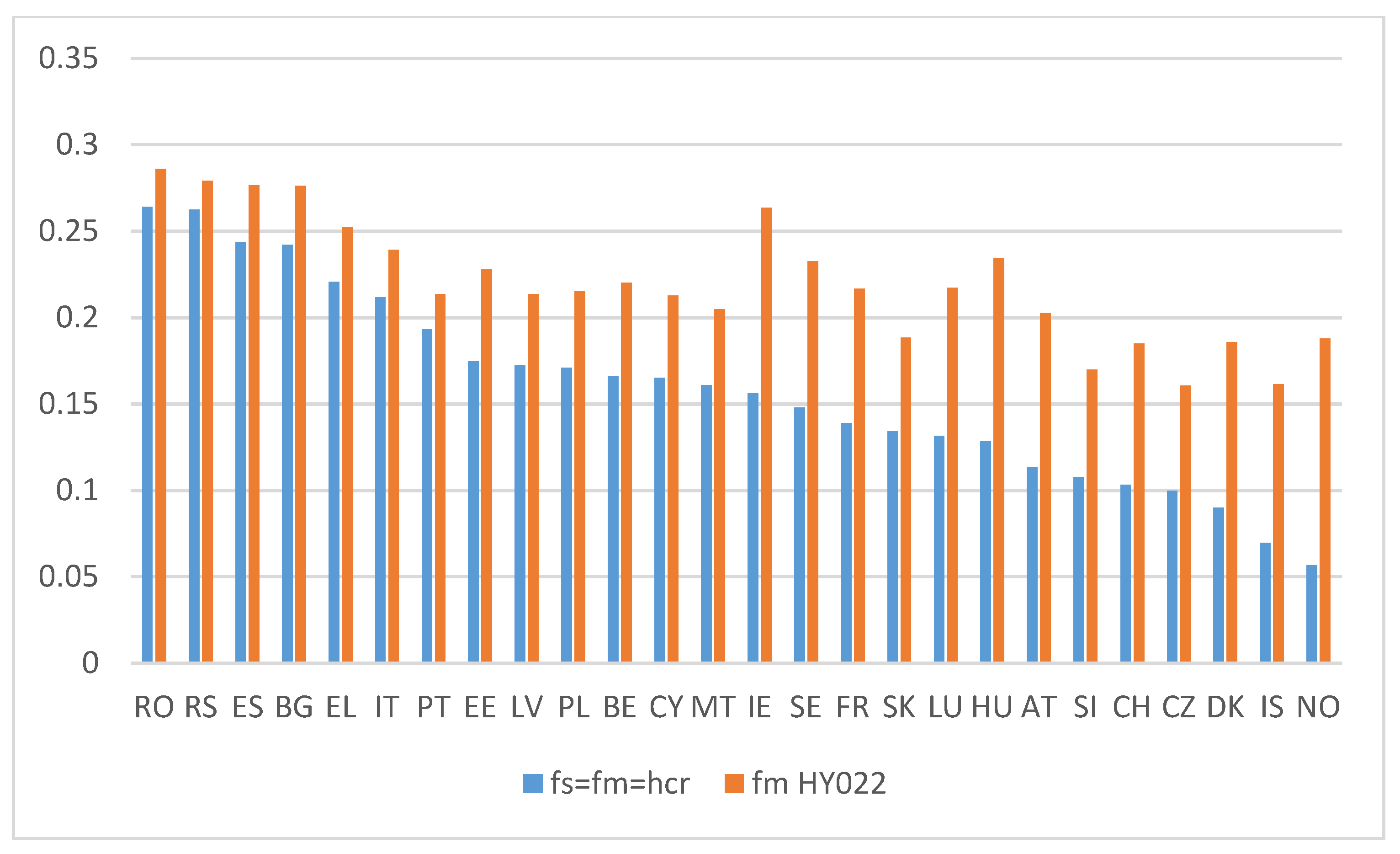
3.1. Fuzzy Monetary Measures

Figure 1 and Figure 2 report a comparison of monetary poverty using two different incomes, namely, equivalized income and income before social transfers for both subsamples.

Observing Figure 1 referring to households with children aged 0–14, the risk of poverty, which was computed considering the equivalized income, is particularly widespread in Bulgaria, Croatia, and Romania, while in Mediterranean countries like Spain, Greece, Italy, and Portugal, it remained substantial; on the other tail of the histogram, we observe significantly lower poverty rates for Scandinavian systems, particularly for Iceland, Norway, and Denmark. The situation is very different if we still examine Figure 1, considering the risk of poverty, computed with income before social transfers: it is evident that the poverty rates for Scandinavian countries now are very similar to those registered by the Mediterranean ones. It seems that considering income before social transfers, the difference in child poverty between Scandinavian and Mediterranean countries narrowed significantly. This issue is consistent with a known situation: social transfers are very different from each other, especially in an international context and in general across countries there have different categories of people, who despite being poor, are not reached by cash transfers. As shown in [10], there are significative differences in regard to the exclusion rates from social transfers among the European regimes. Indeed, the Mediterranean system is the one with the highest exclusion rates for all socio-demographic groups of poor individuals considered; particularly, minors and single parent households in a poverty persistence status report higher non-receipt rates than employed persons. On the other side, Scandinavian countries aim to protect specific categories of the population regardless of the poverty status, so that very small amounts of the poor are excluded. The most protected categories of the poor population, across all welfare systems, are the poor and persistently poor disabled and elderly people.

Now, comparing Figure 1 and Figure 2 and observing Spain, Greece, Italy, and Portugal, we can state that the monetary deprivation considering equivalent income and household disposable income before social transfer is very similar for households with children aged 0–14 or for households with dependent children. It is also evident that in countries with a traditionally strong social assistance system, primarily Scandinavian countries, the monetary deprivation considering household disposable income before social transfer is distinctly higher for households with children aged 0–14. In general, in such countries, the monetary deprivation computed by using disposable income before social transfer is markedly higher for both samples. This remarkable difference is a confirmation that a welfare state can greatly affect households through children’s living conditions.

3.2. Fuzzy Supplementary Measures and Their Precision

As mentioned in the introduction, an added value of the present paper consists in reporting standard errors of fuzzy poverty measures for the subpopulations considered in the analysis. Estimation of variance for complex measures (such as fuzzy ones) from complex surveys (such as EU-SILC) is not a straightforward exercise, and it cannot be performed by standard methods available in usual statistical packages such as SAS, SPSS, STATA, etc. Indeed, while the set of basic assumptions concerning sample design needed to use the variance estimation methods are generally met or they can be reasonably approximated in most population-based surveys, there is an additional one that is often not met in practice [11].

The assumption concerns the availability of all essential information on the sample structure. Indeed, as stated in [5], to compute accurate standard errors for fuzzy measures, it is necessary to have full access to the variables that define the structure of the sample. Here, we needed to adapt the original methodology proposed in [5], due to the lack of sufficient information for the purpose. In fact, the EU-SILC UDB (user database available to researchers) does not contain information on sample structure, in particular concerning stratification and clustering.

Therefore, we used an alternative method by considering the design effect [12], which is the ratio of the variance in a given sample design, to the variance under a simple random sample of the same size. By inverting such a relationship, it is possible to estimate the variance by multiplying the variance in a simple random sample and the design effect. Reference [13] provides accurate estimates of design effects for child poverty for three EU-SILC countries: Austria, Belgium, and Poland.

In

Table 4. Standard errors and confidence intervals: households with children under 14 years old.

Country	Measure	Estimate	Standard Error	CI_Min	CI_Max	Cv
AT	FS	0.113	0.005	0.104	0.122	4.0%
AT	FS1	0.097	0.004	0.088	0.106	4.6%
AT	FS2	0.056	0.004	0.048	0.063	6.7%
AT	FS3	0.079	0.004	0.071	0.087	5.1%
AT	FS4	0.084	0.004	0.076	0.093	4.9%
AT	FS5	0.097	0.005	0.088	0.106	4.8%
AT	FS6	0.099	0.004	0.090	0.108	4.4%
AT	FS7	0.107	0.005	0.098	0.116	4.2%
AT	FS8	0.066	0.004	0.059	0.074	5.7%
BE	FS	0.190	0.006	0.179	0.201	2.9%
BE	FS1	0.156	0.006	0.145	0.166	3.5%
BE	FS2	0.062	0.004	0.054	0.071	7.1%
BE	FS3	0.116	0.005	0.106	0.125	4.3%
BE	FS4	0.124	0.005	0.114	0.133	3.9%
BE	FS5	0.159	0.006	0.147	0.171	3.9%
BE	FS6	0.150	0.005	0.140	0.160	3.5%
BE	FS7	0.165	0.005	0.155	0.176	3.3%
BE	FS8	0.145	0.005	0.135	0.156	3.7%
PL	FS	0.170	0.003	0.164	0.176	1.7%
PL	FS1	0.129	0.003	0.123	0.134	2.2%
PL	FS2	0.055	0.002	0.050	0.059	4.1%
PL	FS3	0.097	0.003	0.092	0.102	2.7%
PL	FS4	0.112	0.003	0.107	0.118	2.4%
PL	FS5	0.114	0.003	0.109	0.120	2.5%
PL	FS6	0.145	0.003	0.139	0.150	2.0%
PL	FS7	0.149	0.003	0.144	0.155	1.9%
PL	FS8	0.154	0.003	0.148	0.160	2.0%

and

Table 5. Standard errors and confidence intervals: households with dependent children.

Country	Measure	Estimate	Standard Error	CI_Min	CI_Max	Cv
AT	FS	0.113	0.004	0.105	0.122	3.7%
AT	FS1	0.094	0.004	0.085	0.102	4.4%
AT	FS2	0.049	0.003	0.042	0.056	7.1%
AT	FS3	0.078	0.004	0.070	0.085	4.8%
AT	FS4	0.083	0.004	0.076	0.091	4.6%
AT	FS5	0.094	0.004	0.086	0.102	4.5%
AT	FS6	0.100	0.004	0.092	0.108	4.1%
AT	FS7	0.107	0.004	0.099	0.115	3.9%
AT	FS8	0.064	0.003	0.057	0.071	5.4%
BE	FS	0.166	0.005	0.156	0.176	3.0%
BE	FS1	0.138	0.005	0.128	0.148	3.6%
BE	FS2	0.047	0.004	0.040	0.054	8.0%
BE	FS3	0.102	0.004	0.093	0.110	4.3%
BE	FS4	0.110	0.004	0.102	0.118	3.9%
BE	FS5	0.142	0.005	0.131	0.152	3.8%
BE	FS6	0.136	0.005	0.127	0.146	3.5%
BE	FS7	0.146	0.005	0.136	0.155	3.3%
BE	FS8	0.131	0.005	0.121	0.140	3.7%
PL	FS	0.171	0.003	0.166	0.176	1.6%
PL	FS1	0.126	0.003	0.121	0.131	2.0%
PL	FS2	0.052	0.002	0.048	0.056	3.9%
PL	FS3	0.097	0.002	0.092	0.101	2.5%
PL	FS4	0.109	0.002	0.104	0.114	2.3%
PL	FS5	0.111	0.003	0.106	0.116	2.3%
PL	FS6	0.142	0.003	0.137	0.147	1.8%
PL	FS7	0.150	0.003	0.145	0.155	1.7%
PL	FS8	0.153	0.003	0.148	0.159	1.8%

, we use these design effects for estimating standard errors for the fuzzy supplementary deprivation measures and their breakdown into the eight dimensions. In most cases, the coefficient of variation (last column) is well below 5%, and, in only a few cases, it is between 5% and 10%. Poverty measures disaggregated for such population subgroups are, clearly, very precise, and such a conclusion could be extended to other countries since their sample sizes were designed so as to get similar standard errors among countries.

These results are in line with the substantive finding of another study [5], according to which, fuzzy measures tend to be subjected to a smaller sampling error than conventional measures of poverty for a given sample size and design. The computation of the standard errors for the fuzzy supplementary deprivation measures actually adds value to the analysis, considering the recommendations of [14], for which standard errors are essential when poverty measures are disaggregated for subpopulations such as children or other groups of interest.

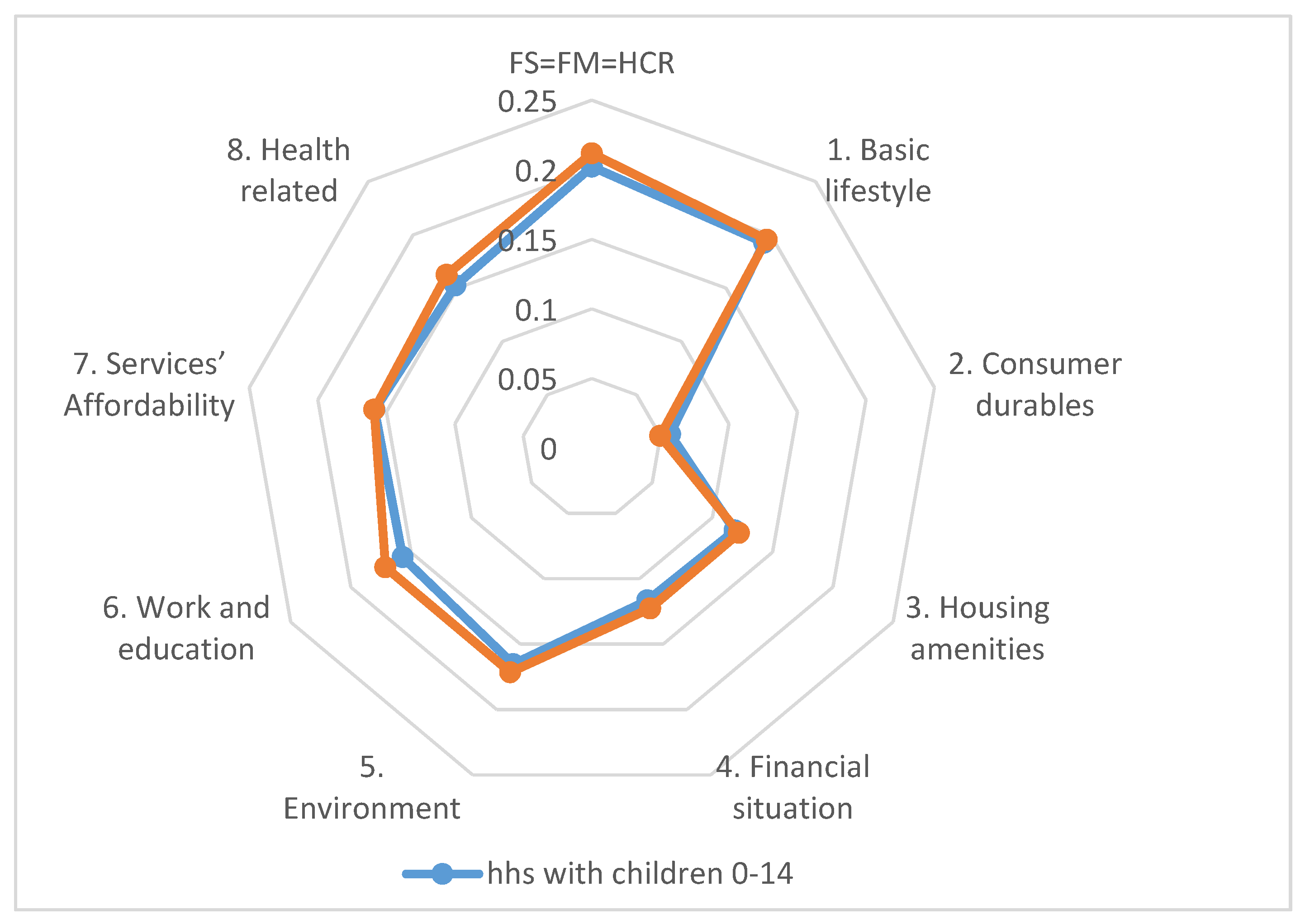
3.3. Comparison of the Two Subpopulations

To compare the deprivation status for the households with children aged 0–14 years and the households with dependent children, a ratio of their scores was computed for each dimension (

Table 6. Fuzzy non-monetary and monetary deprivation: ratios of households with children under 14 years old to households with dependent children.

Country	FS = FM = HCR	1. Basic Lifestyle	2. Consumer Durables	3. Housing Amenities	4. Financial Situation	5. Environment	6. Work and Education	7. Service Affordability	8. Health Related
AT	1.00	1.03	1.13	1.02	1.02	1.03	0.99	1.00	1.04
BE	1.14	1.13	1.33	1.14	1.13	1.12	1.10	1.14	1.11
BG	1.08	1.07	1.09	1.07	1.06	1.03	1.06	1.07	1.03
CH	1.14	1.15	1.19	1.13	1.11	1.12	1.12	1.14	1.12
CY	1.04	1.11	1.34	1.06	1.00	1.02	1.03	1.09	1.05
CZ	1.26	1.28	1.37	1.21	1.22	1.20	1.21	1.26	1.22
DK	1.17	1.20	1.49	1.13	1.20	1.17	1.17	1.17
EE	1.13	1.14	1.21	1.09	1.11	1.08	1.10	1.10	1.10
EL	0.97	0.99	1.03	1.01	1.00	0.96	0.96	1.02	0.97
ES	1.02	1.04	1.09	1.03	1.03	1.02	1.00	1.04	1.02
FR	1.09	1.08	1.23	1.09	1.09	1.07	1.06	1.08	1.08
HU	1.03	1.04	1.05	1.03	1.02	1.05	1.03	1.04	1.04
IE	0.93	0.93	1.25	0.99	0.99	1.02	0.93	0.95	0.95
IS	0.98	1.02	2.07	1.00	1.01	1.04	0.97	1.00
IT	0.95	0.99	1.15	0.97	0.95	0.96	0.92	1.00	0.94
LU	0.97	1.00	1.35	0.99	1.01	0.96	0.95	0.98	1.01
LV	1.11	1.10	1.09	1.06	1.10	1.10	1.09	1.08	1.07
NO	1.71	1.75	2.86	1.56	1.67	1.48	1.59	1.66
PL	1.00	1.02	1.05	1.00	1.03	1.03	1.02	1.00	1.01
PT	1.00	1.01	1.08	1.00	1.00	1.00	0.98	1.01	0.97
RO	1.07	1.09	1.09	1.09	1.03	1.07	1.04	1.06	1.05
RS	1.04	1.07	1.07	1.03	1.03	1.04	1.02	1.05	1.02
SE	1.06	1.08	1.19	1.06	1.09	1.12	1.03	1.06
SK	1.19	1.18	1.18	1.13	1.16	1.11	1.15	1.20	1.19

and

Table 7. Fuzzy monetary deprivation: ratios of households with children younger than 14 years old to households with dependent children.

COUNTRY	FM HX090	FM HY020	FM HY022
AT	1.00	1.15	1.03
BE	1.14	1.19	1.13
BG	1.08	1.05	1.04
CH	1.14	1.08	1.09
CY	1.04	1.07	1.10
CZ	1.26	1.41	1.21
DK	1.17	1.66	1.35
EE	1.13	1.14	1.07
EL	0.97	0.96	1.01
ES	1.02	1.07	1.00
FR	1.09	1.28	1.16
HU	1.03	1.13	1.12
IE	0.93	1.16	1.17
IS	0.98	1.39	1.23
IT	0.95	0.97	0.95
LU	0.97	0.96	0.99
LV	1.11	1.09	1.13
NO	1.71	2.56	1.28
PL	1.00	1.02	1.04
PT	1.00	1.10	1.07
RO	1.07	1.06	1.07
RS	1.04	1.04	1.04
SE	1.06	1.25	1.05
SK	1.19	1.17	1.11

).

Each ratio shows the relative magnitude of the monetary and non-monetary deprivation computed for the two sets of households. Thus, a ratio close to 1 means that the deprivation level is similar to the two sets of households; a ratio greater than 1 indicates that the level of deprivation is higher in households with children aged 0–14 than in households with dependent children aged 0–24; and a ratio lower than 1 indicates that the level of deprivation is higher in households with dependent children than in households with children aged 0–14.

Observing Table 6, we can see that the ratio is generally greater than 1, meaning that the level of deprivation is higher in households with children aged 0–14 than in households with dependent children aged 0–24. For all countries, the ratio of the non-monetary dimension related to consumer durables is greater than 1, meaning that, in all countries, the deprivation level for durable goods is higher in households with children aged 0–14 than in households with dependent children aged 0–24.

It is notable that in three countries, namely Greece, Ireland, and Italy, the ratios are generally lower than 1. This could be explained by considering that these countries have a tradition of large families with children who stay in the household until marriage.

Concerning monetary deprivation, the figures are similar to the non-monetary ones. The ratios are generally greater than 1, meaning that the level of deprivation is higher in households with children aged 0–14 than in households with dependent children aged 0–24 (Table 7). Again, a few countries, namely Greece, Ireland, Iceland, and Luxemburg show ratios lower than 1 with regard to the measure of deprivation related to the household equivalized income (HX090), but only Italy shows ratios below 1 for all three monetary variables.

3.4. Focus on Italy

According to the results presented, from the countries considered, Italy is the only country with all the ratios lower than 1 (except for the dimension of Consumer Durables), meaning that Italy is the only country presenting a higher deprivation for households with dependent children aged 0–24 than for households with children aged 0–14 (see Figure 3).

A consideration that helps in clarifying and understanding the phenomenon, refers to the Italian cultural and social model, in which young people are more likely to live at home with their parents and to accept being without a job or without being in education for a few months; in other words, they accept depending on their parents for a long time. Actually, the average age at which they leave their parents’ home is much higher than in several other European countries. Taken into consideration, this aspect brings together concerns and certainly deserves to be investigated. The analyses presented for all countries were disaggregated by geographical NUTS1 area macro-regions for Italy.

Observing

Table 8. Italian non-monetary deprivation by NUTS1: ratios for macro-regions of households with children under 14 years old to households with dependent children.

	FS = FM = HCR	1. Basic Lifestyle	2. Consumer Durables	3. Housing Amenities	4. Financial Situation	5. Environment	6. Work and Education	7. Service Affordability	8. Health Related
Northwest	0.99	1.02	1.28	0.98	1.02	0.96	0.91	1.05	0.99
Northeast	1.05	1.06	1.43	1.04	1.03	0.96	0.91	1.09	1.05
Centre	0.95	0.96	1.19	0.92	0.91	0.96	0.93	0.96	0.97
South	0.90	0.97	1.21	0.98	0.90	0.94	0.93	0.87	0.82
Islands	1.00	1.02	1.11	1.00	0.91	1.04	0.99	1.07	0.94

, two peculiar patterns are evident: (a) regarding dimension 6, Work and Education, the ratios are below 1 for all the macro-regions; (b) all the ratios are below 1 for all the dimensions (obviously, except for the dimension Consumer Durables) for the Centre and for the South macro-regions.

A serious concern arises from observing pattern (a), considering that in Italy, regarding work and education, regardless of the macro-region in which they are located, households with dependent children aged 0–24 are more deprived than households with children aged 0–14. We could conclude that the added deprivation of the households with dependent children aged 0–24 may be related to a serious and well-known problem, that is, “Not engaged in Education, Employment, or Training” (NEETs).

Indeed, from the literature, Italy is the EU country with the highest percentage of 20–24- and also 20–34-year-old NEETs [15]. Actually, the impact of the NEETs issue is huge since its social cost has been estimated by Eurofound, in 2012 it was 1.2% of Europe’s GDP, but it has a much greater impact in Italy, at 2%.

Regarding pattern (b), only central and southern Italian households with dependent children aged 0–24 are more deprived than households with children aged 0–14 in all dimensions. Actually, the most evident peculiarity regards the South, where the added deprivation of the households with dependent children aged 0–24 is evident for the following dimensions: Financial Situation (dimension 4), Service Affordability (dimension 7), and Health Related (dimension 8). This could be related to uneven development within the country and, therefore, highlight the significant gap between the South and the other Italian macro-regions.

4. Final Remarks

This article investigated multidimensional fuzzy monetary and non-monetary deprivation in households with children using two different definitions: households with children below the age of 14 and the EU definition of households with dependent children (below the age of 24). Following the approach of [7], eight dimensions of non-monetary deprivation were found using 34 items from the survey EU-SILC (2016).

Generally, results show that in most EU countries, households with children below age 14 are more deprived in all non-monetary and in monetary dimensions than households with dependent children. Standard errors of the measures were provided, stating the robustness of the results. For a small group of countries, the results are reversed with respect to those described above. Italy belongs to this smaller group and a particular focus was carried out at a macro-region level. Two main results were determined, as follows: households with dependent children are more deprived in the dimension of Work and Education regardless of the macro-regions, and this may be connected to the high level of NEETs, a widespread, well-known issue in Italy. In southern Italy, the above-mentioned gap is even greater regarding the following three dimensions: Financial Situation, Service Affordability, and Health Related.

Concluding, we highlight that in Italy, to fight children’s deprivation, in addition to the issue of the territorial North–South divide in economic performance, there is a main feature to take into account: the low labor market participation of mothers, as remarked in [16], as well as young adults, which should be an efficient instrument to combat deprivation related to many dimensions analyzed.

References

1. Eurostat. Children at Risk of Poverty or Social Exclusion. 2020. Available online: https://ec.europa.eu/eurostat/statistics-explained/index.php?title=Children_at_risk_of_poverty_or_social_exclusion (accessed on 23 October 2020).
2. European Commission. 2016 EU-SILC Module “Access to Services”; Eurostat: Luxembourg, 2018. [Google Scholar]
3. Zadeh, L.A. Fuzzy sets. Inf. Control 1965, 8, 338–353. [Google Scholar] [CrossRef] [Green Version]
4. Verma, V.; Lemmi, A.; Betti, G.; Gagliardi, F.; Piacentini, M. How precise are poverty measures estimated at the regional level? Reg. Sci. Urban Econ. 2017, 66, 175–184. [Google Scholar] [CrossRef]
5. Betti, G.; Gagliardi, F.; Verma, V. Simplified Jackknife Variance Estimates for Fuzzy Measures of Multidimensional Poverty. Int. Stat. Rev. 2018, 86, 68–86. [Google Scholar] [CrossRef] [Green Version]
6. Betti, G.; Verma, V. Fuzzy measures of the incidence of relative poverty and deprivation: A multi-dimensional perspective. Stat. Methods Appl. 2008, 17, 225–250. [Google Scholar] [CrossRef]
7. Betti, G.; Gagliardi, F.; Lemmi, A.; Verma, V. Comparative measures of multidimensional deprivation in the European Union. Empir. Econ. 2015, 49, 1071–1100. [Google Scholar] [CrossRef]
8. Cheli, B.; Lemmi, A. A Totally Fuzzy and Relative Approach to the Multidimensional Analysis of Poverty. Econ. Notes 1995, 24, 115–134. [Google Scholar]
9. Betti, G.; Cheli, B.; Lemmi, A.; Verma, V. Multidimensional and Longitudinal Poverty: An Integrated Fuzzy Approach. In Fuzzy Set Approach to Multidimensional Poverty Measurement; Lemmi, A., Betti, G., Eds.; Springer: New York, NY, USA, 2006; pp. 111–137. [Google Scholar]
10. Baldini, M.; Gallo, G.; Reverberi, M.; Trapani, A. Social Transfers and Poverty in Europe: Comparing Social Exclusion and Targeting Across Welfare Regimes; Center for the Analysis of Public Policies (CAPP) 0145; Università di Modena e Reggio Emilia: Modena, Italy, 2016. [Google Scholar]
11. Verma, V. Sampling Methods, Training Handbook; Statistical Institute for Asia and the Pacific: Tokyo, Japan, 1991. [Google Scholar]
12. Kish, L. Survey Sampling; Wiley: New York, NY, USA, 1995. [Google Scholar]
13. Verma, V.; Betti, G.; Gagliardi, F. An Assessment of Survey Errors in EU-SILC; Eurostat Methodologies and Working Papers; Eurostat: Luxembourg, 2010. [Google Scholar]
14. UNECE. Poverty Measurement Guide to Data Disaggregation; United Nations: New York, NY, USA; Geneva, Switzerland, 2020. [Google Scholar]
15. Rosina, A. I neet In Italia Dati, Esperienze, Indicazioni per Efficaci Politiche di Attivazione; StartNet—Network Transizione Scuola-lavoro: Roma, Italy, 2020. [Google Scholar]
16. Natali, L.; Saraceno, C. The Impact of the Great Recession on Child Poverty: The case of Italy. In Children of Austerity: Impact of the Great Recession on Child Poverty in Rich Countries; Cantillon, B., Chzhen, Y., Handa, S., Nolan, B., Eds.; Oxford Press: Oxford, UK, 2017; pp. 170–190. [Google Scholar]
Figure 1. Monetary deprivation, households with children aged 0–14: comparison of equivalized disposable income and income before social transfers.
Sustainability 13 09905 g001
Figure 2. Monetary deprivation, households with dependent children: comparison of equivalized disposable income and income before social transfers.
Sustainability 13 09905 g002
Figure 3. Non-monetary deprivation in Italy for the two subsamples: households with dependent children and households with children aged 0–14.
Sustainability 13 09905 g003