The Short-Term Cost of Greening the Global Fleet

Abstract

Decarbonizing maritime transport is among the top priorities of regulators and continuously attracts significant research attention. However, the cost of renewing and greening the fleet has not been explored in detail. To address this gap, the paper provided a bottom-to-top estimation of the financial need associated with decarbonizing the global shipping fleet for the next 5 years, i.e., until 2026. By developing a model focusing on the main asset classes, the paper approximated the expenditure implied in the short-term fleet renewal (newbuilding and vessel demolition) as well as the expenditure linked to retrofitting the existing fleet. The results indicated an aggregate financial need of USD 317 billion until 2026. Thereof, USD 235 billion are associated with building new ships, while USD 114 billion are allocated to retrofitting. Furthermore, proceeds of USD 33 billion can be generated via demolition sales of old tonnage, reducing the total financial burden. The results entail important policy implications, as they document the monetary impact on investors, lenders, and shipping companies regarding distinct segments of the fleet. Considering the declining overall supply of capital towards shipping, the given results provide a transparent account of the absolute financial implications of decarbonization policies.

1. Introduction

The need of reducing the use of fossil fuels in shipping as means to substantially lessen the emissions of carbon dioxide (CO₂) and generally of green-house gases (GHG), as well as the related policies and instruments of the International Maritime Organization (IMO) are widely discussed in the literature and the relevant press [1,2,3]. The policy goal is to achieve a 50% reduction of carbon emissions against the 2008 levels; this target is also quantified as reduction of CO₂ emissions per transport work, as an average across all segments of international shipping, by at least 40% by 2030. However, both the regulatory framework as well as the technical solutions are not fully determined yet; for example, technologies and fuels promoted as technical solutions are not considered in the current set of applicable rules and regulations [4]. In the 76th session of the Marine Environment Protection Committee (MEPC) of the IMO, new regulations, such as the Energy Efficiency Existing Ship Index (EEXI) and Carbon Intensity Indicator (CII) were adopted, while in future sessions they will be finalized.

The above policy goals also dictate the need to renew parts of the fleet that are not expected to comply with the new regulations; new ships, emitting less GHG per transport work, will replace ships that are close to the end of their economic life or the retrofit investment is not justified. In addition, a substantial number of existing ships should install new technologies or retrofit parts of their propulsion plants in order to comply with the stricter set of environmental rules and limits. Therefore, owners and financiers should schedule investments of substantial amounts within the next years in order to meet the policy goals. Considering that UNCTAD estimates the commercial value of the fleet at USD 952 billion [5] and also considering the retreat of banking exposure [6], the total sum will amount to billion of US dollars. In this regard, Hoffmann et al. estimated an excess capital expenditure for new-build ships of up to USD 761 billion in order to achieve maritime carbon targets [7]. Recently, Stopford estimated an amount of USD 3.4 trillions to be necessary as maritime investments [8], i.e., circa four times the value of the existing fleet. Bearing the above in mind, the objective of this work was to estimate the total amount required for the renewal and retrofit of the assets by 2026, as the midpoint to 2030. The analysis period of five years, from 2021 until 2026, was chosen deliberately for two main reasons. First, the time horizon can be adequately anticipated through the 2020 orderbook and is simultaneously long enough for sufficient fleet renewal to occur. Secondly, a period of 5 years appears feasible to practically understand the short- to mid-term financial impact, as opposed to more long-term considerations spanning several decades, as these involve multiple uncertain predictions to be made (such as, e.g., shifts in the fleet composition or fuel mix). Therefore, by deriving the analysis results from the current fleet structure as is, and by providing timely financial implications, the results are regarded as a valuable and practical contribution to the ongoing discourse on maritime decarbonization.

Methodologically, a bottom-to-top approach was followed, similar to the approach of Psaraftis and Kontovas [9]. Amongst other findings, they delivered a specific breakdown of maritime emissions by vessel types and size brackets, which provides guidance for our analysis, too. Similarly, we intended to break down the financial implications of greening the fleet by vessel types and sizes and, therefore, provide results relevant to the industry, while also specifying the impacts on certain sub-segments.

The paper is structured as follows: the next section briefly outlines the recent policy developments. It should be noted that critical examination of the regulation is beyond the scope of this work, as many researchers are contributing on this aspect [10,11,12,13,14]. Nevertheless, a section reviewing related works and literature is offered with the aim to illustrate the gap in the literature, which this work aimed to bridge. In Section 3, the underlying methodology and model assumptions are introduced. The dataset as well as model input parameters are analyzed in Section 4, before the results are discussed in Section 5. The last section concludes and summarizes this work and highlights the paper’s key findings and potential implications.

2. Policy Outline and Literature Review

2.1. Policy Outline

The IMO, as a special agency of the United Nations (UN), supports the UN Sustainable Development Goal (SDG) 13 and takes urgent action to combat climate change and its impacts. The regulatory framework related to the abatement of GHG and, in particular, Annex IV of the International Convention for the Prevention of Pollution from Ships (MARPOL) and its quality as well as its implications are exhaustively discussed in the literature [15,16].

The regulation on CO₂ was introduced in 2011. Resolution MEPC.203 (62) amended MARPOL Annex VI and introduced the Energy Efficiency Design Index (EEDI) and the Ship Energy Efficiency Management Plan SEEMP, a mechanism for operators to improve the energy efficiency of ships by providing guidance on shipboard procedures and practices aimed at improving the energy efficiency and conservation [17]. Polakis et al. provided a thorough analysis on the EEDI [18]. The EEDI is calculated for every new or existing ship, as per the provisions of Regulation 19, based on the formula provided in the Resolution MEPC.245 (66) and the reference lines provided in Regulation 21 in Figure 1. In principle, the estimated EEDI measurement should be below the reference line. Otherwise, measures should be taken to reduce the emission of CO₂ per unit of transport. These reference lines are to be reviewed by the IMO at the given years. Lower reference lines require lower carbon emissions; therefore, operators are obliged to increase the unit energy efficiency.

The initial GHG target of the IMO suggests an average across all segments of international shipping reducing CO₂ emissions per transport work, by at least 40% by 2030, with the goal of 70% by 2050, given 2008 levels as the benchmark; hence, the final objective is to reduce annual GHG emissions from ships by 50% by 2050 [19]. In November 2020, MEPC, in its 75th session, approved amendments to MARPOL Annex VI proposed in October by the IMO’s Intersessional Working Group on Reduction of GHG. These amendments are briefly outlined below:

• The Energy Efficiency Existing Ship Index (EEXI) is introduced from 2023 for all ships of 400GT and above. Practically, every ship should reach a level below the baseline, which is currently equivalent to the reference lines of EEDI Phase 2 or Phase 3 (from 2023/25). Owners can meet this requirement through a range of methods, such as engine power limitation, using alternative fuels, or retrofitting with energy-saving technologies (EST), such as the wind assisted propulsion (WASP) technologies; recent literature provides a thorough overview of WASP technologies and the current status [20,21].
• The Carbon Intensity Indicator (expected to be the Annual Efficiency Ratio (AER) for most ships) is introduced from 2023. All vessels of 5000 GT and above will be required to calculate their AER and they will be allocated a rating on an annual basis. This rating will vary from A to E, with C indicating that a vessel is reducing its carbon intensity in line with the IMO’s intended pathway to reach the global 2030 target; vessels with a rating of D (for 3 years) or E (at any point) will be required to submit improvement plans.
• The EEDI Phase 3 will be brought forward from 2025 to April 2022 for vessel types including containerships, most gas carriers, general cargo ships, and cruise ships (see Figure 1). Reductions of 30–50% from the EEDI baseline will be required under Phase 3 for containerships.

The abovementioned recent measures highlight the regulatory uncertainty. Measures like EEXI and AER introduce new parameters of uncertainty for investors and operators of existing ships. The question generated is simple, and is not rhetorical or fictitious: is a given ship capable to trade as is or does it need retrofits? If retrofits are necessary, will the related investment pay off? The value of the ship as an asset is impacted directly; the question of whether the book value of the asset reflects and approximates market levels is critical for every financial plan and decision. The decision to bring forward EEDI Phases also increases uncertainty for new ships. Albeit, Ross and Schinas proved the interplay of asset prices and environmental regulation and the bias of lenders to finance greener tonnage [22]. Amongst others, these aspects are critical when considering the European effort to shift cargoes from land to sea, a policy with an inherent green objective and other benefits to society. Other regional policies might also be affected, such as the swift change of the fuel mix used by ships or the air quality at ports. Regardless of the fuel or technology selected, current and new ships will demand higher investment vis-a-vis ships of current conventional technology or financial benefits when calling ports that eventually impact the financial performance of the ports [16].

Overall, this poses the question of whether stricter environmental rules will result in more expensive ships and whether capital intensive investments will eventually pay off.

Furthermore, any pricing of carbon might be justified in principle, as externalities are internalized, yet the level of the financial burden might severely impact financial planning and decision-making [7,23].

Last but not least, regional policy initiatives and instruments, such as those of the European Commission that unilaterally pursue measures, especially on carbon pricing, result in further uncertainty in the industry [24].

2.2. Literature Review

As stated previously, many researchers have already analyzed the regulatory framework. Nevertheless, for the needs of this work, two topics were discussed further: the inventory of emissions and the availability of finance. The first issue is important as it relates to scenarios and analyses of the future needs for decarbonizing the fleet, while the latter is important as it shows the availability of debt financing that leverages necessary investments.

2.2.1. Greenhouse Gas Emissions from Shipping

To date, a significant number of emission inventories as well as projections of future maritime emission development have been introduced. While data availability has been frequently criticized as a barrier towards informed decision making, GHG emissions from ships have become increasingly well-explored and documented in the last decade [25,26].

Figure 2 provides a top-level overview of the evolution of maritime CO₂ inventories. It is important to acknowledge the underlying methodological revisions, including the shift from vessel-based to voyage-based estimates in the Fourth IMO GHG Study [27]. Figure 2 thus displays multiple inventory estimates per study, where applicable.

Overall, since 1990, carbon emissions from international shipping have followed a steady growth trajectory, exhibiting temporary emission reductions between 2007 and 2012 [28,31]. As these temporary reductions fall into the analysis period of the Third IMO GHG study, the drivers of these emission reductions are well documented. Amongst other considerations, during the aftermath of the global financial crisis, the fleet exhibited historically low levels of productivity. This concerned both sea-days and operating speeds, as relative excess supply was confronted with low demand, causing significant latent emissions, i.e., in the case of returning demand, a trend reversal was to be expected, considering prior growth in other market fundamentals such as the number of vessels, fleet total installed power, and demand ton-miles, even during the time of low demand [31].

Most recently, the Fourth IMO GHG Study indicated a return towards previous emission growth trends in the latest inventory period [27].

Beyond historic inventories, Figure 3 provides an overview of future CO₂ emission projections towards 2050, retrieved from the Third and Fourth IMO GHG Studies.

This includes a subset of the scenarios established in both studies, filtered by relative importance within the respective publications (see scope of scenarios). Note that Figure 3 only focuses on CO₂ projections, while the IMO envisions cutting all GHG emissions by 50%.

Among the most frequently cited works, the Third IMO GHG Study projected a significant emission growth of up to 250% until 2050 versus 2012 levels under business-as-usual assumptions, inter alia owing to rising transport demand [31]. More recent data from the Fourth IMO GHG Study anticipated reduced CO₂ emission growth estimates towards 2050 in the magnitude of 90% to 130% against 2008 levels [27,33].

However, it can be observed that even the reduced growth outlook falls significantly short of the level of ambition expressed in the IMO’s Initial Strategy to reduce all greenhouse gases from ships, aiming to cut emissions by half until 2050 [32]. Based on the provided Fourth IMO GHG Study mean figures, the emission forecast currently implies a gap of 756 million tons of CO₂ towards the designated 2050 target. Acknowledging this gap, the next section introduces relevant investigations of maritime decarbonization.

The above Figure 2 and Figure 3 clearly demonstrate the relation of the total global fleet, its operating profile, and installed green technology with the expected carbon emissions. The total number of ships directly impacts the carbon inventory, assuming same or similar operating and technology profiles; the higher the number of ships in the water, the higher the expected emissions. In this regard, the greener the operating profile, e.g., the higher the utilization rate of the fleet or segments of the fleet, the lower levels of the abovementioned projections that will be achieved. This is also expected when the fleet uses better fuels or technologies that reduce the unit emissions of CO₂ and other pollutants. Therefore, it is important to conduct a bottom-to-top analysis in order to gain insight per segment and age-group of the fleet.

2.2.2. Decarbonizing the Fleet: Overview of Financial Issues

Besides operational changes, the carbon intensity of the global fleet can fundamentally be reduced in two ways: by replacing old vessels with ships of superior environmental performance (fleet renewal) or by increasing the energy efficiency of existing vessels via retrofit installations [12]. Fleet renewal dynamics, often referred to as the maritime fleet renewal problem (MFRP), are widely discussed as a strategic problem to optimize fleet structures in terms of capacity and vessel mix decisions [34,35,36,37,38,39]. While the MFRP traditionally focuses on static investment decisions to build new ships or retire existing capacities, Pantuso et al. identify the need for adaptive models which can capture empirical market developments, such as novel environmental constraints [40]. The first evidence in this regard was provided by Patricksson et al. who analyzed the MFRP by introducing regional emission limitations to evaluate scrubber retrofit investments compared to low-sulphur fuel usage [41].

In other words, the spectrum of potential fleet investment decisions in the MFRP is expanding, as retrofit installations provide additional complementary solutions to continued investments in more efficient new-builds [42]. In this regard, retrofitting can be defined as the installation of technologically superior components or systems on-board of existing vessels in order to achieve performance improvements or satisfy regulatory requirements, often in terms of environmental efficiency [14,43].

Beyond the wider low-carbon shipping literature, several specific issues in terms of retrofitting existing vessels have been reviewed from various angles. This includes, for instance, considerations of retrofit market ecosystems [44,45,46]. To a large extent, this also relates to a more technical body of retrofit literature [47,48,49,50,51].

The regulatory requirements of greening the fleet were discussed in the previous section, and issues, such as EEDI and EEXI, have already been outlined. Recently, Schinas provided an overview of current financial conditions, as well as of the related financial decision-making approach. Figure 4 illustrates the reduction of lending capacity globally [52].

Available estimations in the literature present an aggregate estimation of the cost of renewing or retrofitting the fleet. Yet, irrespective of single estimates, criticism of the available evaluations refers to an observed lack of vessel-specificity or little attention drawn to the interdependence of measures, e.g., concerning the additivity of abatement potentials. Moreover, the variability of estimated reduction potential itself poses questions about their overall validity. However, the reviewed publications on aggregate support the hypothesis that emission reductions to achieve the ambitious IMO 50% goal are possible, given substantial coordinated efforts [1,14,53].

Beyond reduction potential, the absolute costs as well as the relative cost-effectiveness are well explored for many measures, particularly via Marginal Abatement Cost (MAC) curves [27,54]. However, despite the availability of supposedly cost-effective or even cost-negative measures, empirical technology diffusion is observed to be lower than assumed in prior studies [13]. Accordingly, barriers towards the implementation of more energy-efficient technologies are frequently analyzed [55,56,57].

Related prior research which is of particular importance for the given analysis is provided by Eide et al. and Hoffmann et al. [7,58,59]. Their work includes investigations of the costs of maritime decarbonization scenarios and the implications for the industry’s capital expenditure. For 2010 to 2030, they project excess capital expenses for installing green technology on board of new-build ships between USD 183 billion and USD 761 billion, depending on the applied cost-effectiveness threshold [7]. Their observation that prior research activity largely evolved around cost-effectiveness of emission abatement still appears to be a valid concern today, partially disregarding the absolute financial burden implied in greening investments.

Lately, Stopford provided an estimation of USD 3.43 trillions for the decarbonization of the fleet; the underlying assumptions are not known to the authors [8]. The wide range of estimations, i.e. circa USD 600 billion [7] as well as of USD 3.43 trillions [8], triggered this work, as stated before.

The exhaustive listing of works related to ship finance is beyond the scope of this work; however, the common practices and risk-management approaches, widely accepted in the academia and the industry, are discussed in detail in textbooks [60,61], as well as in recent papers discussing the gap of financing green shipping, such as Schinas et al. [62]. The base case of ship finance projects is a mix of equity and loans, where loans are provided by commercial banks. Therefore, parameters, such as gearing (LTV: loan-to-value ratio), duration, and the cost of loans and capital determine the financial viability of the project. Current market conditions, as well as prudency, suggest an indicative gearing of 50–80%, a duration of 5 to 7 years, and interest (cost of debt) of Libor +350–700 bps. In this regard, an LTV of 70 implies a USD 2.3 loan for every USD 1 of equity; this magnifying effect is needed to attract equity investment in shipping. The reduction of lending capacity as illustrated in Figure 4 also results in a diminished appetite for new projects, such as newbuildings and fleet or technology renewal.

All in all, the literature review first introduced recent volume estimates of historic and projected carbon emissions. Then, relevant works in the context of maritime decarbonization were reviewed, serving as references for the subsequent analysis. Finally, the intersection towards ship finance was briefly introduced. The next section introduces the underlying methodology. Specifically, we established the overall model and its specifications as well as important assumptions made in order to approximate the short-term costs of greening the global fleet, as per our research objectives.

3. Methodology

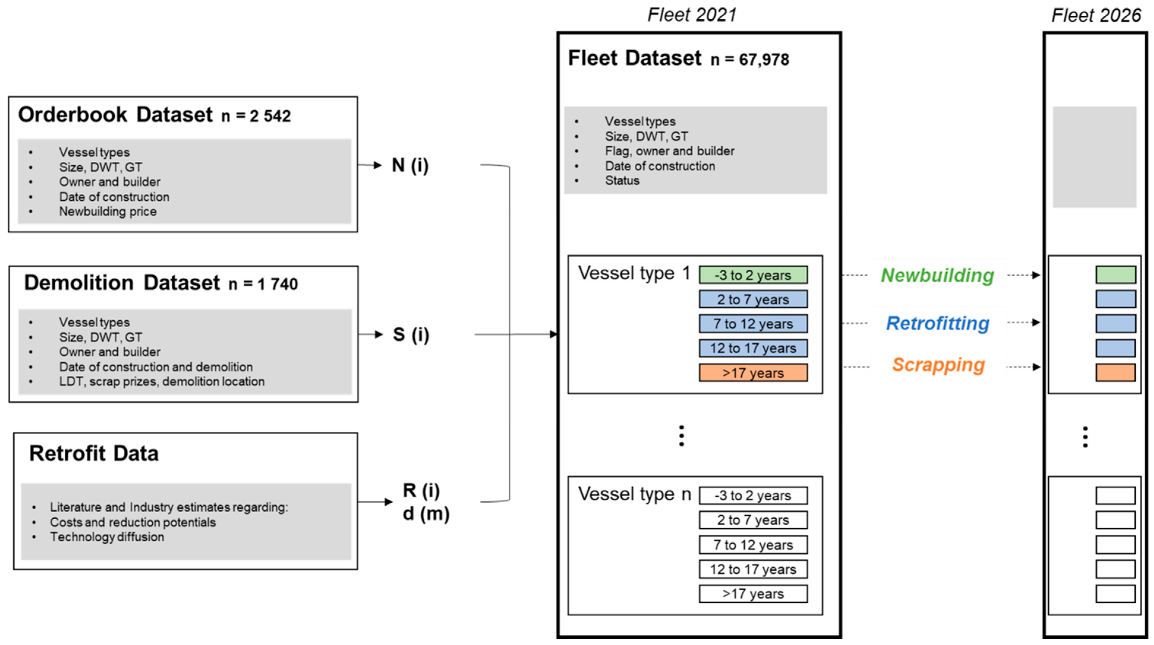
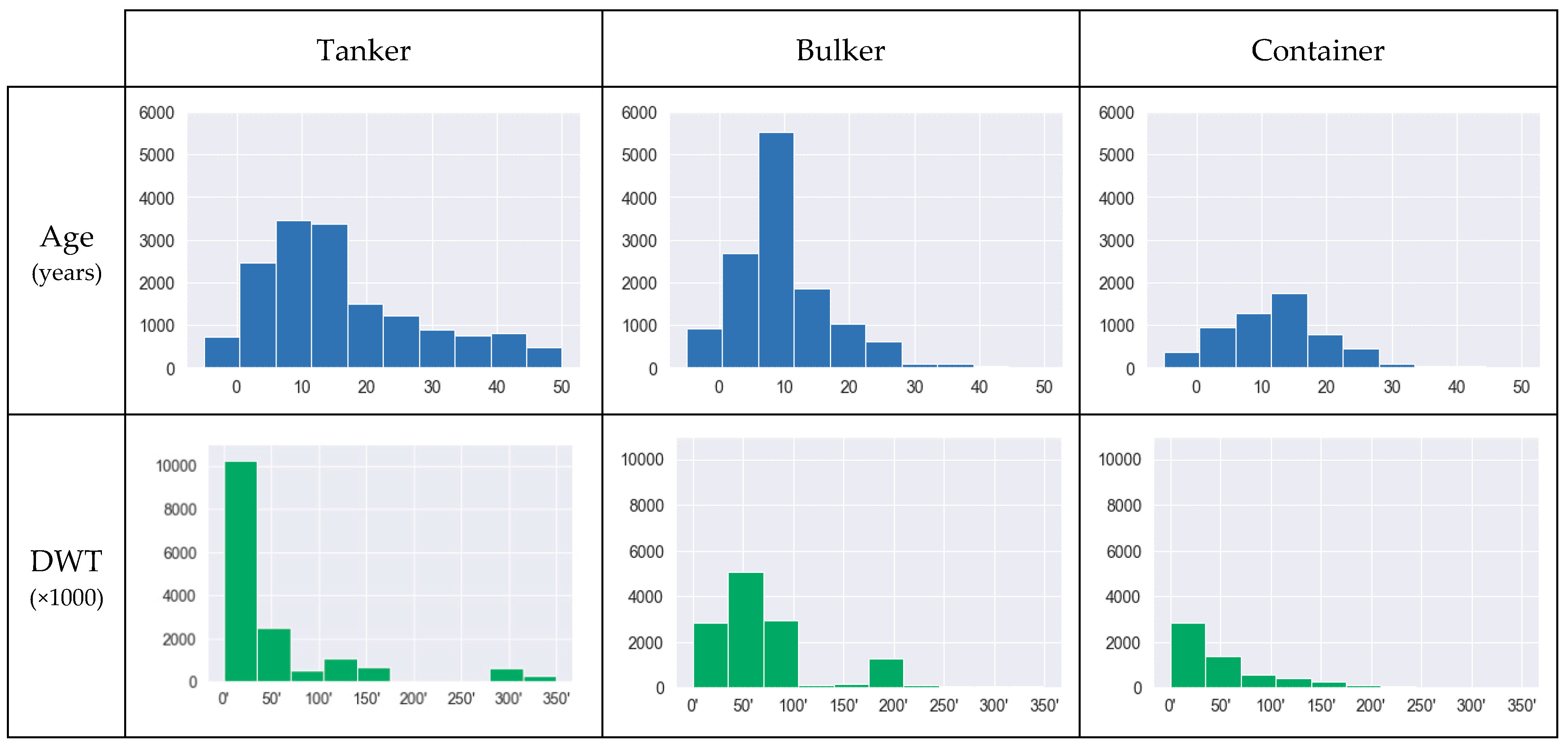
Overall, the paper developed a vessel-based model that builds up on the classification and age breakdown of the global fleet. Figure 5 provides a brief overview of the methodological framework and indicates the relationship between the various datasets employed in the model.

Based on the 2020 fleet structure as documented in the databases of Clarksons’ Shipping Intelligence Network, the model approximated the financial need on the level of each segment, considering their respective age and size profiles. Opposing to, e.g., [7,59], who focus on capital expenditure for building new ships, the analysis explicitly included the expenditure associated with retrofitting the current fleet as well as the revenue generated through demolition sales that usually fuel renewal policies. Notably, the terms scrapping and demolition were used synonymously within the analysis to describe the process of recycling key resources at the end of a vessel’s useful lifetime, in line with prevalent maritime terminology [63,64].

Overall, the model considered a discrete time period of the next five years, i.e., from 2021 to 2026. Thus, the analysis focused on the short- to midterm financial dimension of decarbonizing the fleet. The model differentiated vessels by their age and assigned them to five age groups which determine whether the vessels are eligible for retrofitting, scrapping, or are part of the newbuilding age bin (see Figure 5).

As a direct consequence of the age bin set-up, the average useful economic life of a vessel is defined. It is acknowledged that the analysis of empirical vessel demolition dynamics is itself highly complex and subject to many variables [34,37,64]. Within the model, a uniform age threshold of 22 years was employed, which will be further elaborated on in Section 4. In general, shorter as well longer expected vessel lifetime scenarios can be implemented in the model by iteratively adjusting the age bin structure presented in Figure 5.

On the level of each vessel type, the total costs of decarbonizing the respective fleet segment are divided into the costs of new-build ships $C{\left(i\right)}_{Newbuild}$, the costs for retrofit installations $C{\left(i\right)}_{Retrofit}$, and the income generated through demolition sales $I{\left(i\right)}_{Scrap}$ (see Equations (1) and (2)).

$$Total Costs of Decarbonization={\displaystyle \sum }_{i=1}^n\left(Costs per Vessel Type i\right)$$

(1)

$$Costs per Vessel Type i=C{\left(i\right)}_{Newbuild}+C{\left(i\right)}_{Retrofit}-I{\left(i\right)}_{Scrap}$$

(2)

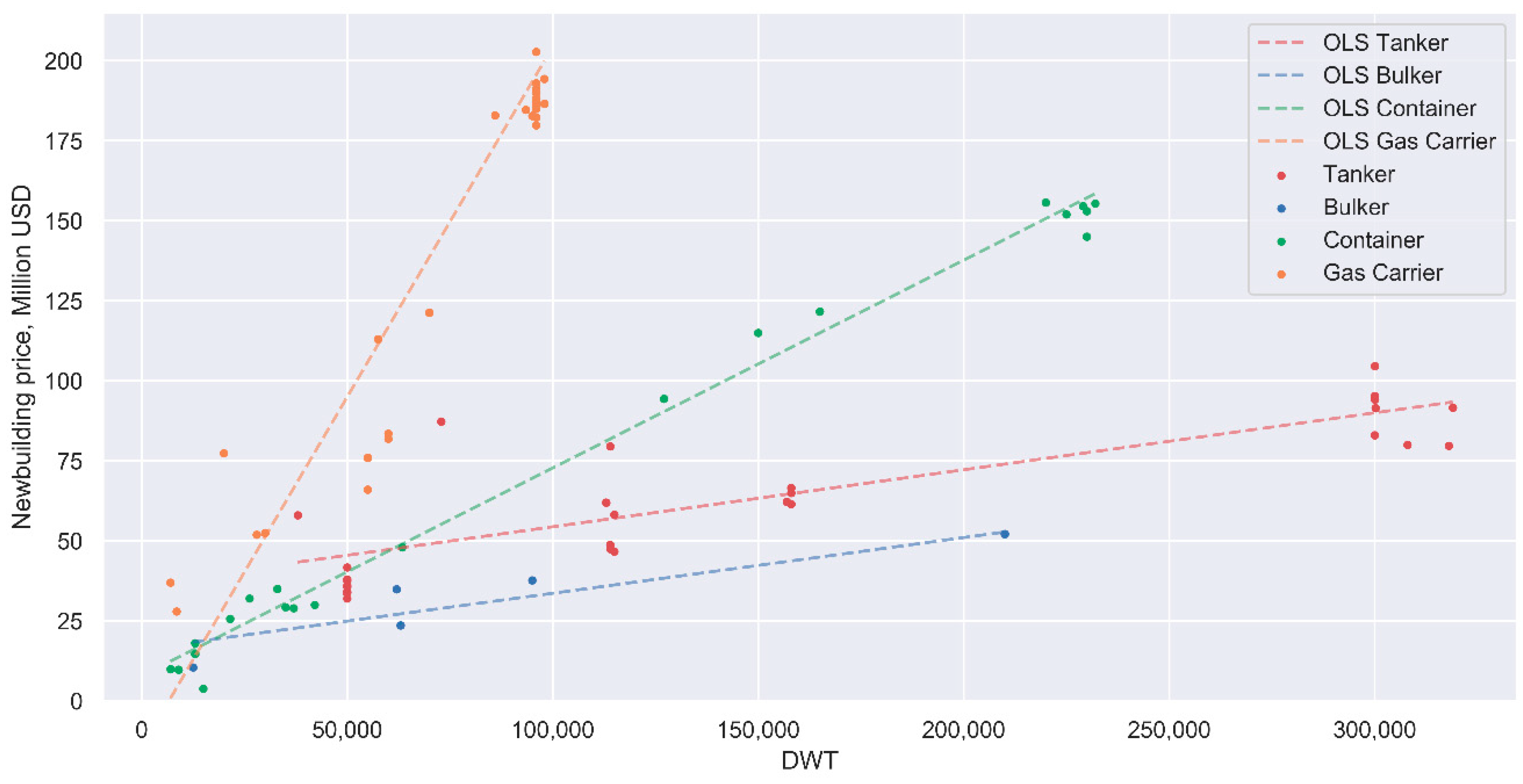
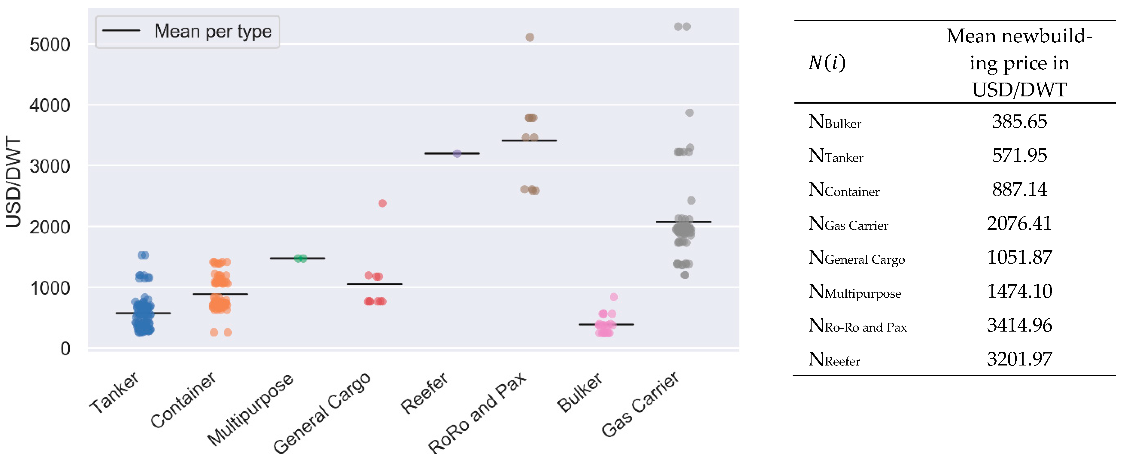
The costs associated with newbuilding (Equation (3)) are subject to the number of ordered ships $n\left(i, m\right)$, the observed price level $N\left(i\right)$, the average vessel deadweight $\overline{\mathrm{DWT}}\left(i,m\right)$, and segment growth expectations$g\left(i\right)$.

$$C{\left(i\right)}_{Newbuild}=n\left(i, m\right)\times N\left(i\right)\times \overline{\mathrm{DWT}}\left(i,m\right)\times g\left(i\right)$$

(3)

where

i = vessel type;

m = age bin;

n (i, m) = number of vessels per type and age bin (−3 to 2y);

N (i) = costs of new-build vessels per type in USD/DWT;

$\overline{\mathrm{DWT}} \left(i,m\right)$ = mean deadweight per vessel type and age bin;

g (i) = growth factor per vessel type.

The estimated retrofit costs (Equation (4)) are represented by the sum of the three age bins eligible for retrofitting. For each bin, the retrofit costs are subject to the price level $R\left(i\right)$, a degressive retrofit diffusion factor between 0 and 1 $d\left(i, m\right)$, the average vessel deadweight, and the number of vessels per type and age bin.

$$C{\left(i\right)}_{Retrofit}={\displaystyle \sum }_{m=2}^4 \left(d\left(m\right)\times n \left(i, m\right)\times R\left(i\right)\times \overline{\mathrm{DWT}}\left(i,m\right)\right)$$

(4)

where

n (i, m) = number of vessels per type and age bin (2 to 7 years; 7 to 12 years; 12 to 17 years);

d (m) = retrofit diffusion factor per age bin [0; 1];

R (i) = costs of retrofit installation per vessel type in USD/DWT.

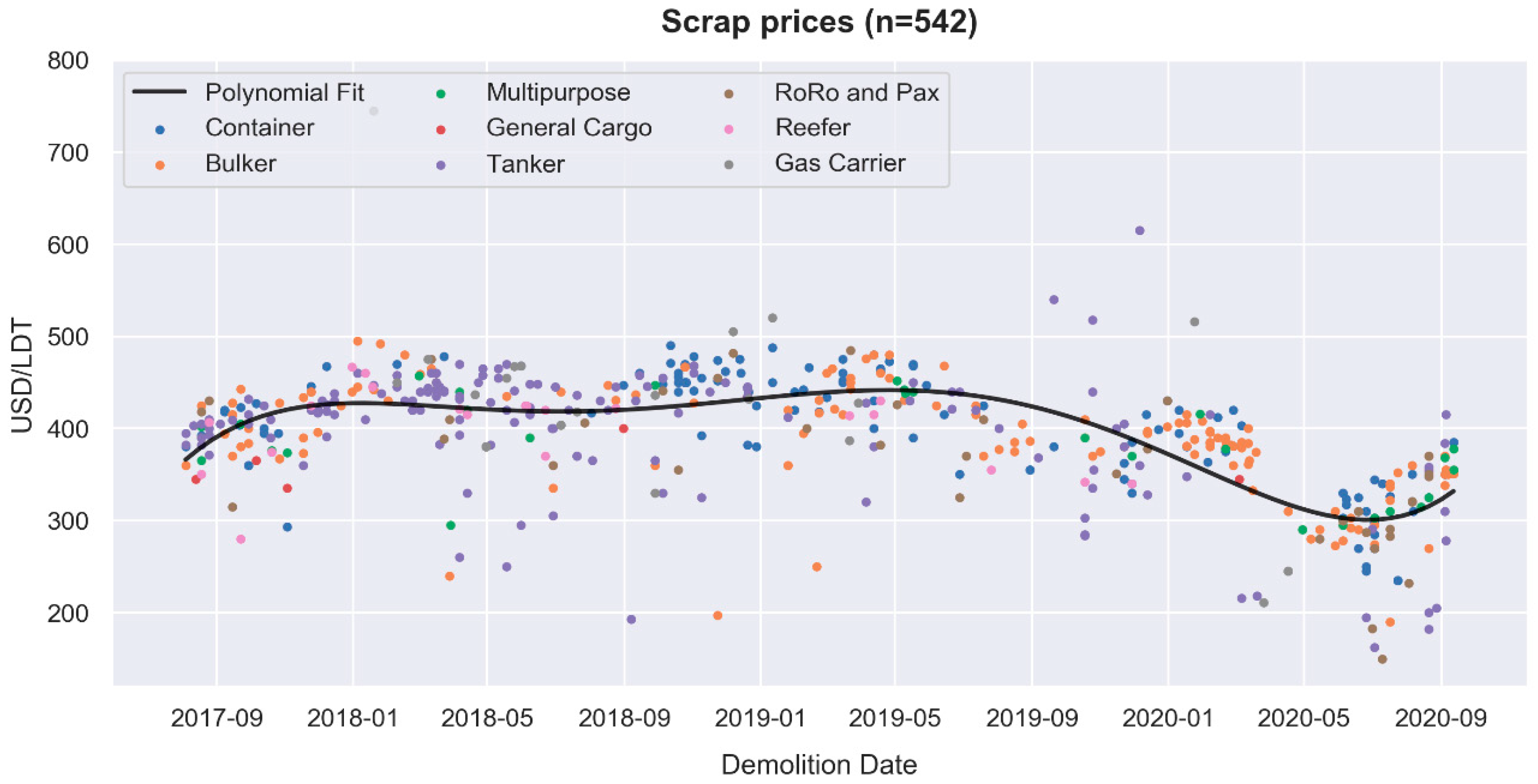
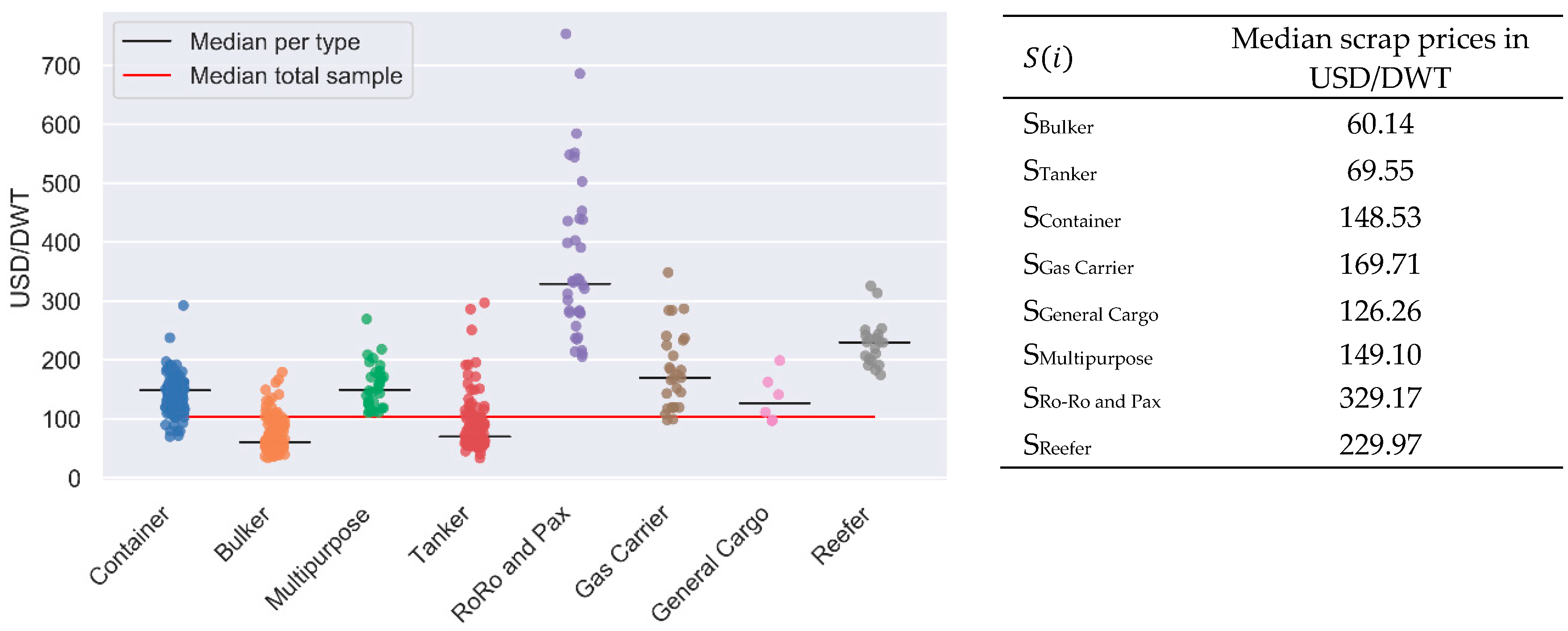
The income generated through demolition sales (Equation (5)) is derived from the number of ships older than 17 years as of 2020 (i.e., whose lifetime exceeds 22 years towards 2026) and is subject to the scrap price level $S \left(i\right)$ as well as the average vessel deadweight.

$$I{\left(i\right)}_{Scrap}= n\left(i, m\right)\times S \left(i\right)\times \overline{DWT}\left(i,m\right)$$

(5)

where

n (i, m) = number of vessels per type and age bin (>17 years);

S (i) = revenue through demolition sales per vessel type in USD/DWT.

4. Data and Breakdown of the Fleet

4.1. Dataset

The relevant world fleet data has been retrieved from the Clarksons Research Shipping Intelligence Network. Similarly to the world fleet breakdown employed by Psaraftis and Kontovas [9], the scope of the analysis focused on all cargo and passenger vessels. This group of ships comprises 95% of the total gross tonnage of the ocean-going fleet and is thus material to international decarbonization efforts and IMO provisions, respectively [9,65]. The following vessel categories are thus excluded from the analysis: offshore, survey units, mobile offshore drilling units, construction vessels/platforms, mobile offshore production units, logistics units, AHTS, PSV, and rescue and salvage vessels.

Table 1. Breakdown of world fleet by vessel types and deadweight. Source: Clarksons Research.

Vessel	No. of Ships	% of Fleet	∑ DWT	% of Fleet
Bulker	12,860	18.92%	964,823,361	44.28%
Handysize Bulker (10,000–35,000 DWT)	2863	4.21%	70,828,354	3.25%
Handymax Bulker (35,000–60,000 DWT)	3856	5.67%	188,734,729	8.66%
Panamax Bulker (60,000–85,000 DWT)	3675	5.41%	270,006,868	12.39%
Post-Panamax Bulker (85,000–120,000 DWT)	650	0.96%	62,378,619	2.86%
Capesize Bulker (>120,000 DWT)	1816	2.67%	372,874,791	17.11%
Tanker	16,320	24.01%	720,712,940	33.08%
Small Tanker (0–10,000 DWT)	8665	12.75%	26,700,838	1.23%
Handysize Tanker (10,000–60,000 DWT)	4407	6.48%	147,421,188	6.77%
Panamax Tanker (60,000–80,000 DWT)	471	0.69%	34,321,739	1.58%
Aframax Tanker (80,000–120,000 DWT)	1166	1.72%	127,388,326	5.85%
Suezmax Tanker (120,000–200,000 DWT)	727	1.07%	112,439,291	5.16%
UL/VLCC Tanker (>200,000 DWT)	884	1.30%	272,441,558	12.50%
Container	5700	8.39%	299,567,449	13.75%
Feeder Containership (0–500 TEU)	356	0.52%	1601,452	0.07%
Feeder Containership (500–1000 TEU)	731	1.08%	7,157,594	0.33%
Handysize Containership (1000–2000 TEU)	1354	1.99%	25,836,273	1.19%
Sub-Panamax Containership (2000–3000 TEU)	765	1.13%	26,590,581	1.22%
Panamax Containership (3000–4400 TEU)	577	0.85%	28,288,914	1.30%
Post-Panamax Containership (>4400 TEU)	1917	2.82%	210,092,635	9.64%
Gas Carrier	2342	3.45%	90,642,249	4.16%
General Cargo	15,586	22.93%	40,156,223	1.84%
Multipurpose	3217	4.73%	30,104,725	1.38%
Ro-Ro & Passenger (incl. PCC)	10,477	15.41%	28,076,091	1.29%
Reefer	1476	2.17%	4,632,785	0.21%
Total	67,978	100.00%	2,178,715,823	100.00%

introduces the world fleet breakdown employed in the analysis. A total of 67,978 ships were in the scope, divided into eight vessel categories.

Furthermore, detailed size brackets are presented for the major vessel types of bulk ships, container ships, and tankers. As shown in Table 1, these represent more than 90% of the global fleet’s deadweight and are consequently of particular relevance for the total model validity. Figure 6 indicates the relevant age and deadweight distributions within these classes.

Besides the world fleet data, information on the newbuilding orderbook as well as vessel demolition for the period from 2017 to 2020 was obtained from Clarksons’ Research.

Table 2. Descriptive statistics for fleet, orderbook, and demolition datasets. Source: authors.

Total Fleet, incl. Orderbook (n = 67,978)
	DWT		GT		Year built		Age
Observations	62,855		66,061		67,978		67,978
Mean	34,662.57		20,813.25		2000.47		19.69
Standard Deviation	57,127.38		33,524.25		16.24		16.31
Min	3		100		1868		−2.96
Max	442,470		337,500		2023		152
Kurtosis	9.64		7.63		2.57		2.58
Skewness	2.84		2.58		−1.32		1.33
Orderbook only (n = 2542)
	DWT		GT		Price USD		Price USD per DWT
Observations	2229		828		333		301
Mean	68,549		30,097		134,023,149		3094.23
Standard Deviation	75,542		49,257		200,857,978		11,011.89
Min	20		101		3,855,000		248.57
Max	400,000		250,000		1,190,000,000		91,086.42
Kurtosis	2.73		4.65		14.86		36.94
Skewness	1.71		2.26		3.77		6.04
Demolition (n = 1740)
	DWT	Year Built	LDT	USD/LDT	USD Total	USD/DWT	Scrap Age
Observations	1731	1740	1059	542	527	527	1740
Mean	43,478	1988.69	12,404	393.24	5,665,769	127.98	29.88
Standard Deviation	67,368	9.94	10,163	73.64	4,560,454	92.48	9.88
Min	15	1925.00	368	150.00	558,445	33.37	5.89
Max	311,176	2012.00	47,342	863.00	20,830,480	753.45	92.58
Kurtosis	5.78	2.45	1.67	6.81	1.28	10.00	2.47
Skewness	2.47	−1.09	1.48	0.46	1.38	2.60	1.09

below presents the descriptive statistics for the three datasets.

Among the descriptive statistics, some observations stand out in particular. These include a noticeable number of vessels exceeding typically observable vessel lifespans, to the point of 20 years or even more (see especially tankers, Figure 6). These will be addressed throughout the discussion. Yet, it may be already noted that while the absolute number of respective vessels is considerable in the dataset, only a small fraction of the global fleet’s deadweight is affected.

4.2. Defining the Model Parameters

4.2.1. Vessel Demolition

As introduced, the model applied an age threshold of 22 years as a basis for the useful economic lifetime of vessels in the analysis. Historically, the useful economic lifetime of vessels is considered to range from 25 to 30 years [63]. Among other downward forces, overcapacity and depressed freight rates may substantially reduce the observable vessel lifetime temporarily [66]. Besides, environmental pressure is expected to affect vessel demolition dynamics, e.g., via scrapping subsidies as analyzed by [64]. The 22 years employed in the given model are furthermore in line with recent industry practices observable in financial institutions dealing with shipping assets [67].

For the period between 2017 and 2020, demolition data for 1740 vessels is available. Thereof, 542 records include price information, which are shown in Figure 7. Within the market, demolition prices are quoted in US dollars per light displacement tonnage ($\frac{\mathrm{USD}}{\mathrm{LDT}}$). As an indication of the price trend across single observations, a polynomial of degree five is fitted to the scrap price timeseries based on a least square approach, using date ordinals as input.

The first observation is that the scrap price quotes in the sample did not vary by vessel types considerably. This finding is supported by standard market practice, where the scrap price is measured in USD per long-ton of the metallic structure, i.e., the sum of all weights, namely of the hull, machinery, and outfitting. Indicatively, refer to the Baltic and International Maritime Council (BIMCO) standard contract template for the sale of vessels for the purpose of demolition and recycling (“DEMOLISHCON”), specifically Clause 12 [68]. Any finding deviating from this practice would spark concerns.

This observation is confirmed by additional demolition panel data beyond the sample scope, displayed in Figure 8. It shows that various scrap price series across vessel types, size brackets, and demolition locations are, on aggregate, highly correlated. Without delving deeper into the analysis of correlation or even causation, it may therefore be reasonably concluded that time constitutes one key driver of the observed demolition prices, while both vessel types and demolition locations show little to no relation towards prices. All in all, the high correlation factors imply indifference to the ship type and the reasonable differences are attributed to the peculiarities of ship types to be recycled, such as the recycling of piping for tankers, coating of ballast tanks, etc.

When disaggregating the granular scrap price data (in $\frac{\mathrm{USD}}{\mathrm{LDT}}$) by vessel types, the prior observation of time being the core driver of demolition income can be confirmed. All vessel types exhibited a similar absolute price range between 200 and 500 US dollars per light displacement tonnage (Figure 9a), which coincides with the associated short-term sample time-series amplitude (Figure 9b) and also the long-run panel data series (Figure 9c).

Besides, the median price of each vessel type approximates the full sample median price, supporting the notion of evenly distributed scrap prices across different types (Figure 9a).

These observations indicate that there are two possible approaches to derive inputs for the income from vessel demolition. Keeping in mind that the model operates on a deadweight basis, one option is to explicitly include a universal projected scrap price level in US dollars per light displacement tonnage ($\frac{\mathrm{USD}}{\mathrm{LDT}}$) in the model, which requires a subsequent conversion to conform with the deadweight-based modelling. Secondly, instead of establishing an exogenous scrap price level (in $\frac{\mathrm{USD}}{\mathrm{LDT}}$), the other option is to explicitly derive the necessary input from the demolition price records and the respective vessel deadweight. Since the latter is more straightforward and a comparative analysis indicates little sensitivity, option two was applied.

Acknowledging the consistency of the available demolition data with long-term observable prices and also the variability of scrap prices over time, the price inputs on a deadweight-basis can be retrieved from the demolition dataset directly. These were approximated as the median scrap prices per deadweight on the level of each vessel type (Figure 10). Figure 10 also shows that, across types, there is a larger variability in the prices on a deadweight basis compared with prices per light displacement tonnage. This boils down to the relationship between deadweight tonnage and light displacement tonnage for each vessel, subject to the distinct technical vessel design characteristics. Thus, for more heterogeneous classes, this results in a wider range of observations.

4.2.2. Newbuilding

The new build price information was obtained from the orderbook dataset (vessel-level) and validated with a larger set of longitudinal price data on the level of vessel types. An important underlying assumption for the analysis is that the orderbook newbuilding prices sufficiently reflect vessel designs capable of supporting maritime decarbonization.

This assumption, is amongst others, grounded in the applicability of the IMO energy efficiency design index (EEDI) to newbuild ships [17]. For a general introduction, see, for instance, Psaraftis [11]. While the regulation itself is not without criticism, the increasingly tight energy efficiency requirements via the EEDI reference lines suggest a positive relationship towards improved environmental performance [22]. Further analyses find an overall increase in vessel design efficiency between 2009 and 2016, while also pointing out a temporary trend reversal for certain vessel types and a notable number of non-compliant new-build vessels [69]. In this context, Stevens et al. argued that reduced design speed and reduced vessel weight are primary outcomes of the EEDI regulation, as opposed to the use of novel technology [70].

From the orderbook dataset (n = 2542), 333 vessel records include price data. Thus, a considerable number of new-build orders does not entail price records. To ensure reliable model inputs, the sample price implications were therefore validated with further exogeneous new-build price information throughout the section.

For various vessel types in the orderbook sample, a linear relationship between the vessel deadweight and the newbuilding price can be observed. Figure 11 plots these relationships for tankers (newbuilding orders for shuttle tankers have been excluded here, because of their over-representation within the orderbook dataset compared to the relevant population), bulk carriers, container ships, and gas carriers, including indicative ordinary least squares (OLS) regression outcomes.

$$\begin{gathered} OLS Regression Line Container: f\left(x\right)=0.00065x+7.85 ({\mathrm{R}}^2=0.99) \\ OLS Regression Line Bulker: f\left(x\right)=0.00017x+16.23 \left({\mathrm{R}}^2=0.88\right) \\ OLS Regression Line Gas Carrier: f\left(x\right)=0.0022x-14.51 \left( {\mathrm{R}}^2=0.74\right) \\ OLS Regression Line Tanker: f\left(x\right)=0.00018x+36.62 \left({\mathrm{R}}^2=0.71\right) \end{gathered}$$

Measured by the coefficient of determination (R²), the observable linear relationships are weakening for vessel types which exhibit stronger intra-class heterogeneity, i.e., classes containing less uniform vessel profiles. This can be noted for tankers (R² = 0.71), which incorporate various size brackets from small tankers up to Ultra Large Crude Carriers (ULCCs). The same holds true, e.g., for the Ro-Ro and Passenger segment, partially involving relatively diverse vessel profiles (not shown in Figure 11).

Given the orderbook data availability for all vessel types and their distribution in comparison with the existing fleet, it has proven particularly useful throughout the analysis to compute the mean price per deadweight on a vessel level, instead of deriving necessary parameters from regression considerations (see Figure 12).

The use of mean orderbook prices as model inputs shall be briefly compared to the presumed linear regression predictions introduced before to validate whether there exist potential systematic errors (

Table 3. Regression prediction versus orderbook mean newbuilding prices. Source: authors.

			(i)	(ii)	(iii)
Vessel Type	Regression Equation	R2	Mean Orderbook Deadweight per Type	Regression Prediction for (i), USD/DWT	Mean Orderbook Newbuilding Price, USD/DWT	Absolute Error, USD/DWT	Relative Error, in % of (iii)
Container	$f\left(x\right)=0.00065x+7.85$	0.99	69,205.65	763.43	887.14	123.71	13.94%
Bulker	$f\left(x\right)=0.00017x+16.23$	0.88	96,653.92	337.91	385.65	47.74	12.38%
Gas Carrier	$f\left(x\right)=0.0022x-14.51$	0.74	60,702.18	1960.96	2076.41	115.04	5.54%
Tanker (excl. Shuttle)	$f\left(x\right)=0.00018x+36.62$	0.71	80,962.70	632.30	571.95	−60.35	−10.55%

).

For the presented vessel types, the newbuilding price implications (in $\frac{\mathrm{USD}}{\mathrm{DWT}}$) deviate from the regression predictions in a magnitude of 5.54% to 13.94% versus the orderbook mean. Both positive as well as negative deviations are observable, reducing the aggregate bias for the total analysis. These deviations may be regarded as acceptable, given the exploratory analysis objective. Nevertheless, to ensure that the model inputs are representative for the total relevant vessel population, the orderbook-based considerations were cross-validated with newbuilding panel data beyond the given sample in

Table 4. Mean orderbook newbuilding prices versus the five-year average ¹. Source: Clarksons Research.

Vessel Type	Unit	5-Year Average 2	Orderbook Mean Price	∆ in %
Container	USD/TEU	11,073.81	10,452.80	−5.94
Bulker	USD/DWT	389.66	385.65	−1.04
Tanker	USD/DWT	525.58	571.95	8.11
Gas Carrier	USD/CBM	1232.11	1248.04	1.28
MPP	USD/DWT	1311.31	1474.10	11.04

¹ Unavailable timeseries include Reefer (not reported), General Cargo (discontinued 2011), as well as Ro-Ro and Pax (available time-series insufficiently reflects segment composition). ² This includes various single-size bracket time-series per vessel type.

. The validation data were retrieved by computing the newbuilding prices from reference ships provided by Clarksons Research.

Overall, the employed newbuilding prices based on the orderbook were in line with the long-term price ranges exhibited in Table 4, especially considering regular newbuilding price fluctuation. Taking into account both the regression outcome as well as the newbuilding panel data, the input parameters retrieved from the orderbook mean prices can be regarded as reasonable approximations which allow for uniform processing of all vessel types.

As a proxy for the short- to mid-term fleet growth projections per vessel segment $g\left(i\right)$, Clarkson’s growth estimates for the year 2021 will inform the model input parameters. For vessel segments where these are unavailable, the preceding three-year-weighted average on a deadweight basis is computed as a substitute (

Table 5. Vessel segment growth factors. Source: Clarksons Research.

$\mathit{g}\left(\mathit{i}\right)$	2021 YoY Growth, in %	3-Year-Weighted-Average Growth (2018–2020), in %	Compounded Growth (2024 to 2026), in %
gBulker	1.4	n.a.	2.81
gTanker	2.2	n.a.	4.44
gContainer	3.0	n.a.	6.09
gGas Carrier	6.9	n.a.	14.27
gGeneral Cargo	n.a.	1.21	2.43
gMultipurpose	n.a.	−0.35	−0.70
gRo-Ro and Pax	n.a.	1.77	3.57
gReefer	n.a.	−2.74	−5.56

). These growth factors must be compounded towards 2026. However, considering the lead time from order to build of approximately 2–3 years [63], a large portion of the segment growth is already covered by the orderbook dataset explicitly. Thus, only the residual model time period from 2024 to 2026 not yet captured in the orderbook must be adjusted. Notably, this presumes a continuation of prior fleet development trends, as shown in Table 5.

4.2.3. Retrofitting the Existing Fleet

In order to estimate the financial need associated with retrofitting the existing fleet, two main model parameters must be specified. On the one hand, the costs of a technology agnostic proxy for retrofit technologies $R\left(i\right)$ was estimated for the global fleet. On the other hand, scenarios about the diffusion $d\left(i, m\right)$of such technologies for different vessel ages were established. These required model inputs were derived from the literature and industry estimates which provide indicative investment profiles for a range of technologies. Notably, these are subject to many variables in practice, including vessel types, sizes, routes, or even trades served [56]. Thus, deriving price implications, regardless of the stack of technology employed, was recognized as a significant simplification.

To approximate investment amounts across vessel types, wind-assisted propulsion (WASP) upgrades were used as an indicative technology benchmark. The propulsive potential of wind energy for new-builds and retrofits has been frequently reviewed [71,72,73,74,75,76,77]. A respective overview of the current technology status as well as future potentials of wind propulsion solutions was submitted to the IMO for the 75th session of the MEPC by Comoros [21]. A practical review of recent applications of wind energy as a source of propulsion is provided by Chou et al. [20].

For the given analysis, a Flettner Rotor served as a starting point because the interaction with the total operating system of the vessel can be well-understood across ship types. Despite limited disclosure of performance and price data, based on industry estimates, a Flettner Rotor suited to support the operations of a 25 k DWT bulk carrier can be installed at approximately USD 2.5 million (all inclusive, no off-hire compensation).

The use of WASP technology as benchmark serves the purpose of providing reserved estimations. As per the IMO (MEPC75/Inf26), the potential of the use WASP technologies is huge due to the need of swift and efficient and relatively inexpensive retrofit towards greening operations. The average reported price per installation is circa USD 2.5 million; given this price benchmark, the cost of other technologies should range close to this market benchmark. The assumption in this work is technology-agnostic, so there is no implied promotion of any technology.

The same cost dimensions can be assumed for tanker and container ships of the same size. Based on considerations of the respective design properties of the remaining vessel types, 30% higher costs may be reasonably assumed. Consequently, bunker fuel reductions in the magnitude of 6% to 12% are realistic, while for container ships, reductions close to 6% may be expected empirically. These considerations are in line with the emission reductions reported in [20,21].

Table 6. Retrofit prices in US dollars per deadweight. Source: authors.

$\mathit{R}\left(\mathit{i}\right)$	Retrofit Prices in USD/DWT	Reduction Potential
RBulker	100	6–12%
RTanker	100	6–12%
RContainer	100	6%
RGas Carrier	130	6–12%
RGeneral Cargo	130	6–12%
RMultipurpose	130	6–12%
RRo-Ro and Pax	130	6–12%
RReefer	130	6–12%

summarizes the implied retrofit prices on a deadweight basis as well as the corresponding indicative reduction potentials.

Compared to the above 25 k DWT benchmark vessels, a cost degression must be considered for ships of growing size. Equipping, for instance, a 75 k DWT bulk carrier with two Flettner Rotors (investment USD 5 million), a retrofit price of 66.67 USD per deadweight is implied. Thus, such degressive retrofit cost inputs must be tested in the scenario-based modelling.

Table 7. Indicative evidence of different retrofit project profiles.

Source	Measure	Vessel	Nominal Investment USD	Implied USD/DWT	Reduction Potential
[20]	Flettner rotor	Various implementations	n.a.	n.a.	0.4–50.0%
	Kites	Various implementations	n.a.	n.a.	1.0–50.0%
	Wing sails	Various implementations	n.a.	n.a.	5.0–60.0%
[54]	Towing Kites	10–20 k DWT Chemical Tanker	987,100	65.80	4.6–9.2%
	Integrated propeller and rudder upgrade	5–10 k DWT General Cargo Ship	415,360	55.38	2.0–6.0%
[48]	Retrofit power plant	12,350 DWT Ro-Ro cargo ship	n.a.	n.a.	n.a.
[72]	Flettner rotor	9700 DWT Ro-Ro vessel	n.a.	n.a.	5.0%
[78]	Flettner rotor	109,647 DWT Product Tanker	n.a.	n.a.	8.2%
[42]	Bundle of fuel efficiency retrofit technologies	46 k DWT Bulk Carrier	1,000,000	21.73	n.a.
	Dual fuel engine switch	46 k DWT Bulk Carrier	10,000,000	217.39	n.a.

presents an overview of further references towards similar retrofit project profiles. It must be noted, however, that data availability constitutes a main challenge in this regard, i.e., even among the scarce references available, all necessary input variables are only seldomly made public (vessel type and size, nominal investment amount, and realized/anticipated emission reduction potential). Thus, in the absence of a wide array of public cost and performance data, establishing transparent benchmark parameters underpinned our approach, which will be complemented by additional scenario-based modelling.

Besides the price level of retrofit technologies, the diffusion of the respective technology per age bin $d\left(m\right)$ is an important model parameter. The penetration of retrofit installations was regarded as a decreasing function of a ship’s age, given a shorter remaining lifetime of the vessel, and consequently reduced investment payback times [79]. Although reported payback times deviate across publications, ranges between 1 and 3 years [42] or 0.5 and 10 years [28] are documented, depending on the respective technology stack. Thus, given relatively short breakeven intervals for several technologies, a large share of the fleet is fundamentally eligible for retrofit considerations.

Rehmatulla et al. provided empirical evidence on the implementation of technical energy efficiency and CO₂ abatement technologies [13]. Although they did not control for vessel age, the reported penetration rates on a measure-basis provide a reference for our model, ranging from 1% (use of solar energy) up to 89% (contra-rotating propellers). No implementations of wind-assisted propulsion upgrades were recorded for the survey sample. Similarly, the Fourth IMO GHG Study estimates upper- and lower-bound technology penetration rates, which can inform the analysis [27].

In general, there are various arguments supporting comparatively slow technology uptake scenarios. For instance, the industrialization and large-scale adoption of low-carbon technologies appears to lag behind the academic debate [1,14,53]. However, in this context, the analysis objective should be recalled. Estimating the financial dimension of the decarbonization pathways implied in the IMO level of ambition explicitly includes technology penetration rates exceeding empirically documented levels.

The technology diffusion rates employed in the model as base case inputs are displayed in

Table 8. Retrofit technology diffusion rates. Source: authors.

$\mathit{d}\left(\mathit{m}\right)$	Diffusion
d2–7 years	100%
d7–12 years	70%
d12–17 years	40%

. These represent the presumed share of vessels being retrofitted in the respective age brackets for each vessel type. The modelling includes iterations of both higher as well as lower diffusion rates, while the fundamental notion of diffusion being a degressive function of age remains unchanged.

5. Analysis of Results

5.1. Estimated Financial Need of Short-Term Decarbonization

The previous sections have documented the search for appropriate model inputs in detail, resulting in the specified base case estimates. These will be applied and extended through modelling further scenarios. To reduce the number of potential variable combinations, clusters of variables (e.g., retrofit price levels across different vessel types) were altered simultaneously as relative deviations from the base case parameters (see

Table 9. Model scenario overview: base case scenario and variations. Source: authors.

No.	Scenario	Short Description	Newbuild	Scrapping	Retrofit		Growth Rates
			N(i)	S(i)	R(i)	d(m)	g(i)
I	Base Case	Best available estimate: subject to the parameter specifications developed in previous sections.	See Section 4.2 for all introduced base caseparameters per vessel type.
II	Lower Bound	Lower bound scenario given by joint reductions in all variable clusters by 10% (Note: inverse relationship for scrapping).	−10%	+10%	−10%	−10%	−10%
III	Upper Bound	Upper bound scenario given by joint increases in all variable clusters by 10% (Note: inverse relationship for scrapping).	+10%	−10%	+10%	+10%	+10%
IV	Retrofit Industrialization	Higher retrofit technology penetration within the fleet, costs of technology are falling (learning and economies of scale), slightly reduced scrap prices.	c.p.	−5%	−20%	+20%	c.p.
V	Low Retrofit Price Level	Univariate degression of retrofit price level towards price implications of two Flettner Rotor case introduced above (66.67$\frac{\mathrm{USD}}{\mathrm{DWT}}$).	c.p.	c.p.	−33.33%	c.p.	c.p.
VI	Increased New-build Activity	Increase in fleet segment growth rates (newbuilding); paired with slight decrease in scrap price levels, assuming steady fleet capacity and thus slight increase in vessel demolition.	c.p.	−10%	c.p.	c.p.	+20%
VII	Newbuilding Substitutes Retrofitting	Stronger relative emphasis on efficient new-builds to achieve decarbonization objectives.	c.p.	c.p.	c.p.	−20%	+20%
VIII	Retrofitting Substitutes Newbuilding	Stronger relative emphasis on retrofitting existing ships to achieve decarbonization objectives.	c.p.	c.p.	c.p.	+20%	−20%
IX	Increased Scrap Price Level	Univariate increase in scrap price level, for instance via a scrapping subsidy as discussed in Yang et al. (2019)	c.p.	+20%	c.p.	c.p.	c.p.
X	Decreased Scrap Price Level	Univariate decrease in scrap price level.	c.p.	−20%	c.p.	c.p.	c.p.
XI	Reduced Retrofit Diffusion	Lower penetration rates for retrofit technology, subject to the respective age bins.	c.p.	c.p.	c.p.	75/50/25%	c.p.

). These scenarios served as an indication of the different model outcomes for variable combinations which deviate from the base case settings (as specified in previous sections). As shown in Table 9, the scenarios represent uni- and multivariate modifications of the original model, which are intended to account for various sources of fluctuation in the relevant markets, affecting the respective model variables.

Notably, particular attention is drawn to the base case model output as well as lower and upper bound implications. The further scenarios will not be discussed individually but are represented by means of the total value ranges.

Using bulk carriers as an example, the model application shall briefly be demonstrated. The Equations (2)–(5) introduced in Section 3 and the base case parameters for bulk carriers imply the following calculations:

$$\begin{array}{l}C{\left(Bulker\right)}_{Newbuild}=1468\times 385.65\frac{\mathrm{USD}}{\mathrm{DWT}}\times 96,810.20\mathrm{DWT}\times 1.0281\approx \mathrm{USD}56,347,658,661\\ C{\left(Bulker\right)}_{Retrofit}=100\%\times 2727\times 100 \frac{\mathrm{USD}}{\mathrm{DWT}}\times 80,498.90 \mathrm{DWT}+70\%\times 5120\times 100 \frac{\mathrm{USD}}{\mathrm{DWT}}\times 75,484.70 \mathrm{DWT}\\ +40\%\times 1657\times 100 \frac{\mathrm{USD}}{\mathrm{DWT}}\times 69,512.18 \mathrm{DWT}\approx \mathrm{USD} 53,613,034,390 \\ I{\left(Bulker\right)}_{Scrap}=1888\times 60.14 \frac{\mathrm{USD}}{\mathrm{DWT}}\times 53,772.31 \mathrm{DWT}\approx \mathrm{USD} 6,105,645,301\\ C{\left(Bulker\right)}_{Total}=\mathrm{USD} 56,347,658,661+\mathrm{USD} 53,613,034,390-\mathrm{USD} 6,105,645,301=\mathrm{USD} 103, 855,047,750\end{array}$$

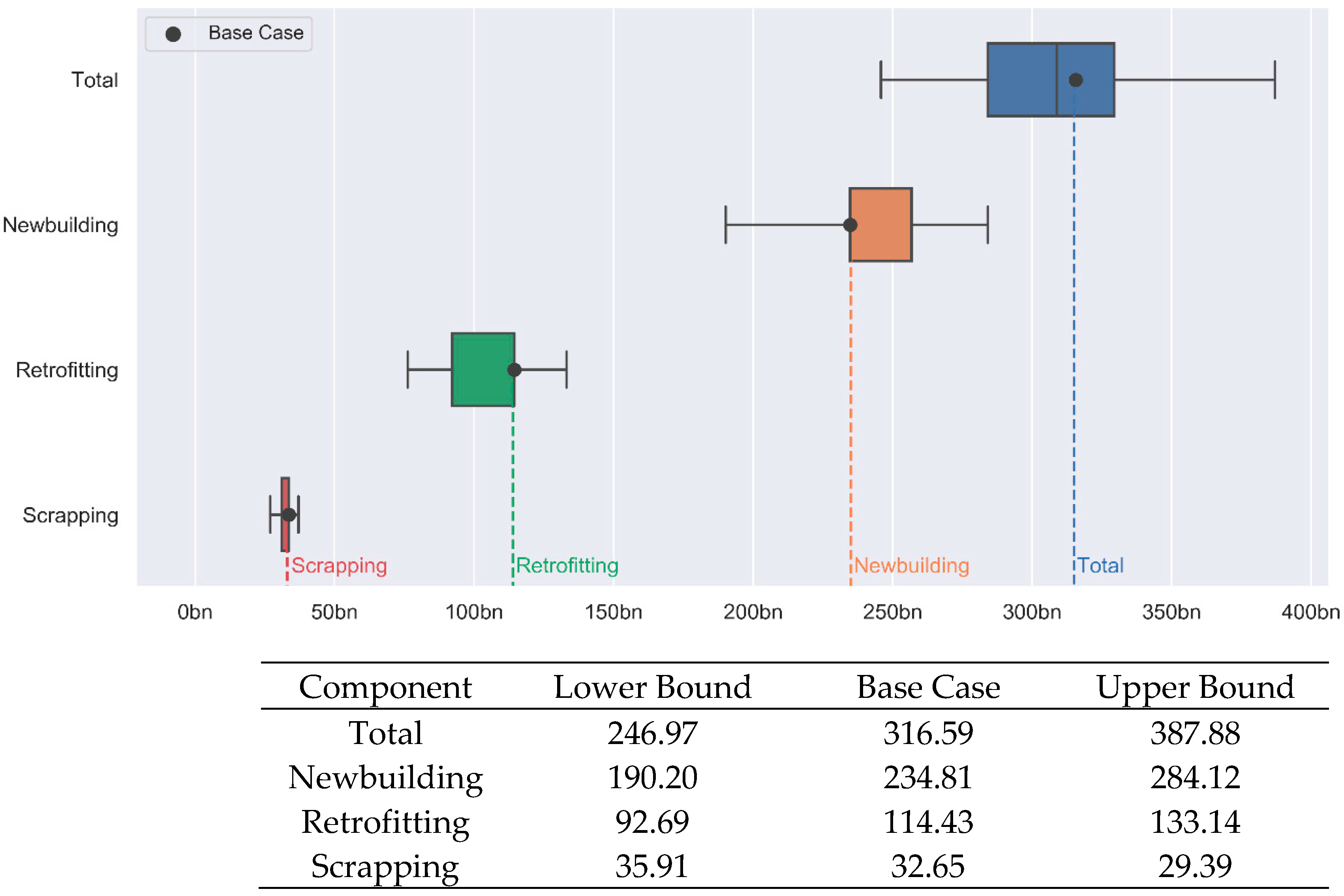
By replicating this logic for all vessel types and iterating over the introduced scenarios, the final modelling results can be derived. The results are presented in Figure 13, breaking down the total model estimate of the financial need into its subcomponents.

Until 2026, the aggregate financial need is estimated at USD 317 billion, which arises from building new ships and retrofitting existing vessels minus the income generated through demolition. Thereof, the largest share of USD 235 billion is allocated to building new ships, while the estimated costs of retrofitting amount to USD 114 billion. The income generated through vessel demolition sales is estimated at USD 33 billion.

Given the base case parameters, the need for capital per year therefore equals USD 63 billion until 2026. In total, the upper as well as lower bound estimates imply a financial need of USD 247 billion and USD 388 billion, respectively. To put these figures into a maritime business context, one may consider the total commercial value of the world fleet, estimated at USD 952 billion in 2020 [5]. Thus, the projected aggregate financial need for capital (USD 317 billion) represents roughly 33% of the respective world fleet value. 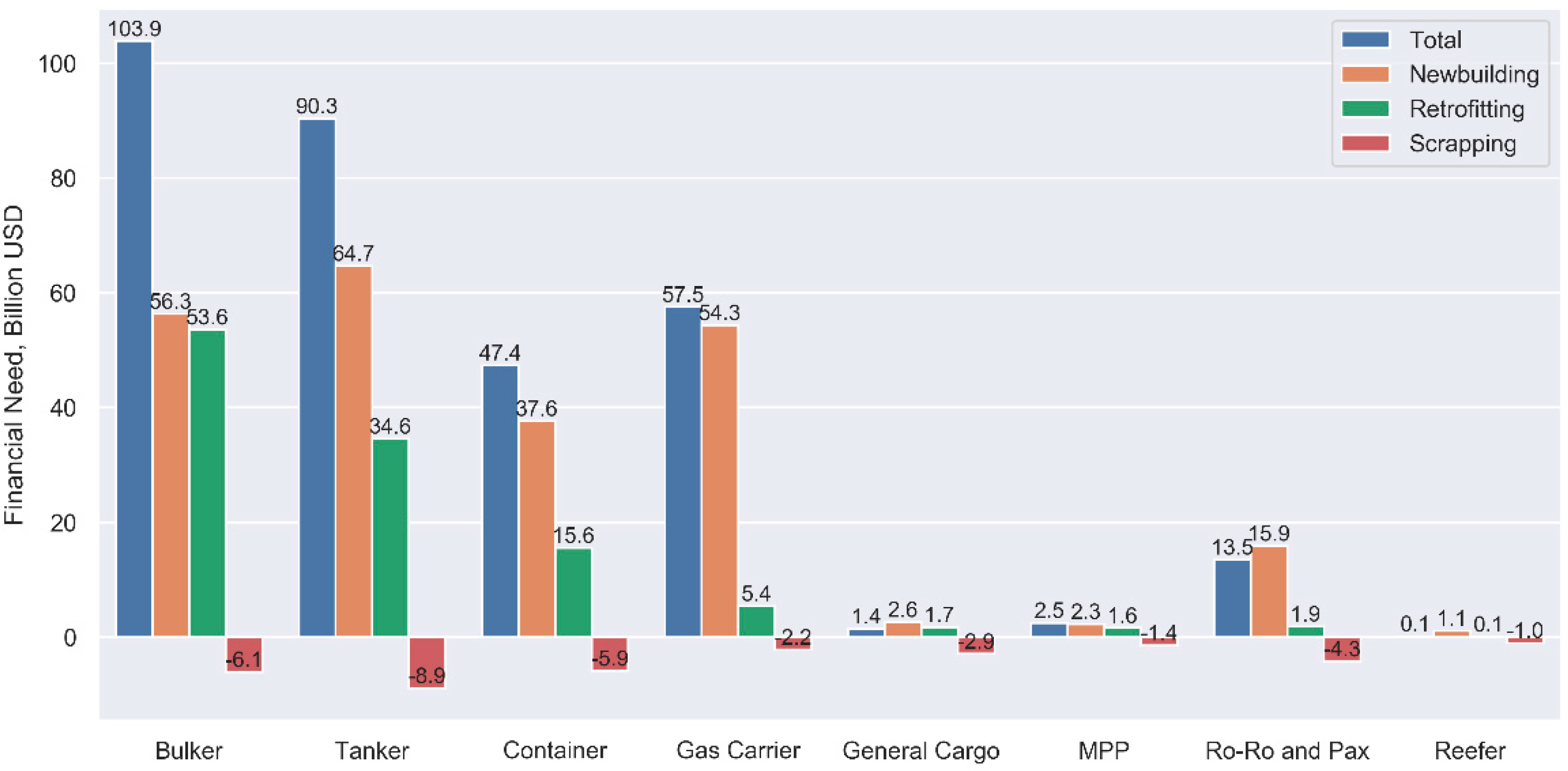Figure 14 disaggregates the total financial need by newbuilding, retrofitting, and scrapping for each vessel type.

Accordingly, the largest share of the financial burden relates to bulk carriers, tankers, and container ships, as well as gas carriers. For the gas carrier segment, the capital need is primarily attributed to newbuilding, driven by full orderbooks and high segment growth expectations as well as high overall asset values. The same holds true for the Ro-Ro and passenger segment.

As defined, the income generated through vessel demolition reduces the overall financial burden. Yet, the magnitude of this effect is relatively insignificant compared to the overall financial dimensions. On the level of single vessel types, though, the respective impact can be proportionally bigger. This includes clusters with higher relative age profiles such as general cargo ships, which are scrapped more frequently according to the model definition.

Moreover, the modelling results can be further broken down up to the level of single age brackets per vessel type (see Appendix A). Additionally, the full breakdown provided in Appendix A differentiates vessels below and above 30 k deadweight as a proxy for short-sea shipping. Given the most recent policy dynamics in regulating maritime emissions, this perspective may be of political interest, as predominantly short-sea shipping may be affected by the EU ETS in the future. Unsatisfied with the regulatory progress within the IMO, the European Parliament envisions an extension of the EU ETS scope to include shipping in the carbon trading scheme [80].

5.2. Analysis Results Versus the Supply of Capital

Finally, the absolute estimates provided above do not yet answer the question of whether the maritime financial markets can satisfy the inherent need for capital. Thus, the following section discusses the results in relation to the current international ship finance environment.

Considering the central role of debt financing and especially syndicated loans for ship finance, the absolute need for capital may further be translated into the required contributions of lenders. Based on the loan-to-value (LTV) conditions prevalent in the market, the implied debt requirements can be derived [81]. Commonly, newbuilding projects are financed with higher LTV ratios than observable for retrofit initiatives. On aggregate, a large portion of shipping loans is provided at LTV ratios between 60% and 80% [82].

Of the total projected need for capital (USD 317 billion), USD 235 billion have been associated with newbuilding projects and USD 114 billion with retrofit investments. Given that the proceeds from scrapping vessels (USD 33 billion) are split proportionately to finance respective newbuilding or retrofit projects across the fleet, this results in the reduced financial need for debt capital, shown in

Table 10. Debt requirements of maritime decarbonization for different LTV conditions in billion USD. Source: authors.

		LTV Retrofit
		0.65	0.6	0.55	0.5
LTV Newbuilding	0.75	227.07	221.88	216.70	211.51
	0.7	216.43	211.24	206.05	200.87
	0.65	205.78	200.60	195.41	190.22
	0.6	195.14	189.95	184.77	179.58

below.

The absolute amounts and value ranges shown in Table 10 imply debt requirements per year between USD 36 billion and 45 billion until 2026. As a reference point for the total industry credit exposure, the top 40 shipping lenders accumulated a total exposure of USD 294 billion towards shipping in 2019 [6]. Thus, the total predicted financial need until 2026 under base case assumptions (USD 317 billion) exceeds the aggregate loan portfolio of these banks by roughly USD 22 billion, whereas the specific requirements for debt shown in Table 10 fall below this indicative benchmark. Overall, this illustrates the magnitude of the financial challenge. Yet, a more meaningful conclusion can be drawn from analyzing dynamic flows of capital.

Kavussanos and Visvikis [83] as well as Schinas [52] provide an overview of the fresh capital provided to shipping annually over time. Since 2010, the total capital inflow (incl. private equity, bank debt, public equity, and bonds but excl. bilateral loans) per year can be observed at approximately USD 80 billion on average. More recent data regarding the volume of syndicated loans towards maritime industries further specifies the allocation of debt towards shipping companies (see

Table 11. Syndicated loans towards maritime industries in billion US dollars. Source: Clarksons Platou Structured Asset Finance.

	2017	H1 2018
Shipping	41.6	14.0
Offshore	22.2	15.6
Shipyards	6.7	3.2
Total	70.4	32.8

).

Leaving aside additional sources of funding, two preliminary conclusions can be drawn by comparing the analysis results with the high-level indicators regarding the availability of maritime capital. First, the results indicated that the underlying financial burden of decarbonizing the fleet is substantial. While this finding alone appears trivial, quantifying these efforts has proven more complex. Secondly, despite the substantial financial burden, it can be concluded that the estimated financial need is within reach of historically observable levels of capital endowment.

Therefore, this supports the overall notion that decarbonizing the fleet bears significant financial challenges which in turn do not appear irresolvable, given its estimated financial dimension. In this regard, any potential financial gap apparently widens once predictions closer to the upper bound modelling results materialize. Likewise, the results are subject to the short-term development of the supply of capital towards shipping.

5.3. Sensitivity Analysis

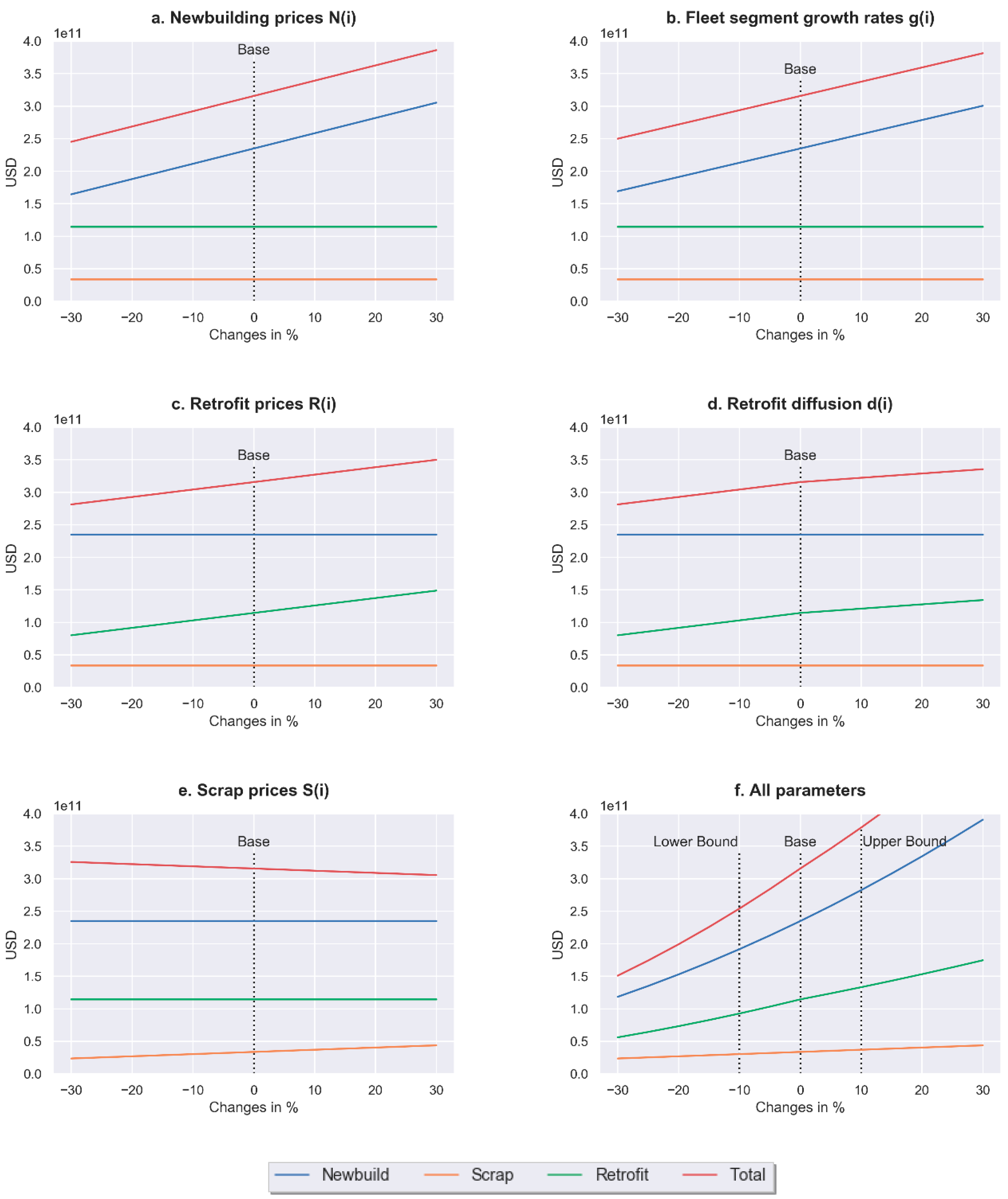
While the range of the different scenario model results already provides an overview of the fundamental model dynamics (see Figure 13), the sensitivity towards changing parameters shall be reviewed more systematically. The subplots provided in Figure 15 below document the impact of symmetric deviations from the base case settings.

More precisely, clusters of variables (e.g., newbuilding prices $N\left(i\right)$ in $\frac{\mathrm{USD}}{\mathrm{DWT}}$) were modified simultaneously as relative variations from the base case, while the other variables remained constant.

On aggregate, the sensitivity towards changes was highest for variations in the newbuilding components, i.e., price levels and fleet segment growth. Apparently, changes in both clusters of variables have the same impact on the model outcome, since they affect the same model equations (Figure 15a,b). Given the fact that newbuilding initially accounts for a larger share of the total output compared with retrofitting, the respective leverage is naturally higher. However, the relative impact of increasing newbuilding price levels is also higher compared with equivalent changes in the retrofit price levels (Figure 15a,c). This is further documented in

Table 12. Sensitivity towards relative changes in variable clusters. Source: authors.

Variable Cluster	Relative Change vs. Base Case	Impact on Aggregate Financial Need
		Absolute, USD Billion	Relative
Retrofit prices $R\left(i\right)$	−10%	−11.44	−3.63%
	+10%	+11.44	+3.63%
Retrofit diffusion $d\left(m\right)$	−10%	−11.44	−3.63%
	+10%	+6.60	+2.09%
Scrap prices $S \left(i\right)$	−10%	+3.27	+1.03%
	+10%	−3.27	−1.03%
Segment growth $g\left(i\right)$	−10%	−23.48	−7.44%
	+10%	+23.48	+7.44%
Newbuilding prices $N\left(i\right)$	−10%	−23.48	−7.44%
	+10%	+23.48	+7.44%

below, providing numerical evidence of the sensitivity towards changes by ten percent for each of the variable clusters.

6. Conclusions, Limitations and Policy Implications

Decarbonizing maritime transport constitutes a key priority to international shipping. The corresponding emission targets are set by the IMO, and policy instruments designed to achieve these targets are continuously evolving, as described. At the same time, the financial implications of the implied decarbonization pathways are rarely analyzed in the literature. Among the very limited available estimates which quantify costs of compliance, methodologies and outcomes diverge significantly.

In order to address this gap in the literature, this paper approximated the short-term cost implications of maritime decarbonization. Methodologically, we follow a bottom-to-top approach considered in the literature for similar estimation problems. More precisely, we developed a vessel-based model which distinguishes financial effects caused by vessel newbuilding, retrofit investments, and vessel demolition sales for the years 2021 to 2026. Further, the model computes relevant financial implications on the level of vessel types and age brackets, up to the level of single vessels. Therefore, besides the absolute financial dimension, the paper contributed towards understanding the distribution of the financial burden towards different segments of the world fleet.

The results indicated a total financial need of USD 317 billion for decarbonizing the global fleet until 2026, given the specified base case conditions. Per year, these figures imply a need for capital of USD 63 billion to build new ships and retrofit existing vessels, less the income generated through demolition sales. Based on prevalent loan-to-value conditions, this translates to yearly debt requirements between USD 36 billion and USD 45 billion.

Based on a brief review of the current ship finance market environment and the available funding opportunities, two partial conclusions were derived. First, in absolute terms, the estimated financial need is substantial, representing a material challenge for maritime businesses. This notion is further reinforced by the ongoing contraction of shipping loan portfolios overall. At the same time, the financial burden may be regarded as moderate on an industry-level for two main reasons. On the one hand, the estimated financial need is within reach of historically observable levels of capital financing, as explored especially for debt capital. On the other hand, the provided estimates appear as moderate in comparison with other available projections.

The provided results contribute to the literature as they add another methodological perspective, since especially retrofit considerations have been underrepresented in the very few similar analyses available. Among other methodological differences, the results can be regarded as of high practical value for the ongoing discourse on maritime decarbonization, considering the short-term analysis period as well as the model design which builds upon the currently observable world fleet structures and newbuilding orderbook.

Several limitations of the study should be considered. One core challenge of the analysis relies on the heterogeneity of the fleet itself. The methodological approach intended to capture the heterogeneous nature of the fleet via the distinction of vessel types, age brackets, and size profiles. In this regard, deadweight was employed as the central variable throughout the full analysis. Notably, certain dynamics are not directly addressed by the deadweight-based modelling. For instance, these include the finding of Ross and Schinas, who documented that superior energy performance is more frequent in vessels of higher commercial value relative to its market share in deadweight [22]. This may be regarded as a proxy for similar phenomena which are not directly embodied in the deadweight-based approach.

In general, the validity of the input parameters was closely monitored and further validated with complimentary panel data for both newbuilding and vessel demolition components. Thus, the risk of biased model input parameters was reduced to a minimum, but can hardly be eliminated entirely, especially for vessel types which exhibit stronger intra-class heterogeneity.

Among the limitations which result from the methodological set-up, time plays an important role. This relates to both the time horizon of the analysis as well as the end-of-life assumption for all vessels in the modelling. The analysis period of five years from 2021 until 2026 was chosen deliberately for two main reasons. First, the time horizon can be adequately anticipated through the 2020 orderbook and is simultaneously long enough for sufficient fleet renewal to occur. Secondly, a period of 5 years appears feasible to practically understand the short- to mid-term financial impact, as opposed to more long-term considerations spanning several decades.

The second time-related question evolves around the age bin structure, which directly implies the presumed end of life for all vessels. While the notion behind the end of life for vessels at 22 years was introduced in prior sections, it must be acknowledged that this results in potential upward bias for certain parts of the fleet. This is true for vessel types which do not fully adhere to competitive renewal cycles observable for other segments and thus exhibit comparably old age distributions, as for instance the General Cargo segment.

However, this effect can be regarded as insignificant for the total model outcome. While a considerable number of 15,910 vessels are reported to be older than 30 years in our dataset, they only makes up 1.77% of the world fleet’s deadweight. Therefore, the deadweight-based modelling places little emphasis on this fraction of the fleet. Moreover, even when factoring in the risk of upward bias for this distinct model component, the financial equivalent of vessel demolition only accounts for roughly one tenth of the total model estimate, thereby having a negligible effect on the overall results.

Furthermore, this work offered necessary insights for further policy considerations. As per the findings of Table 10, the total sum required for a smooth transition, circa USD 300–350 billion, equals the total available lending capacity reported. More aggressive decarbonization policies will result in higher scarcity of capital. Therefore, the demand and supply of ship finance capital will be distorted, and the higher cost of capital should be expected. Should this be the case, then only some projects, mainly the riskier ones that yield higher returns, will be selected. Consequently, a lack of funding for segments with relatively lower yields such as of coastal shipping will occur, despite their critical importance in decarbonizing transportation networks. This aspect is critical when considering the European effort to shift cargoes from land to sea, a policy with an inherent green objective and other benefits to society. Other regional policies might also be affected, such as the swift change of the fuel mix used by ships or the air quality at ports. Regardless of the fuel or technology selected, current and new ships will demand higher investment vis-a-vis ships of current conventional technology or financial benefits when calling ports that eventually impact the financial performance of the ports. Therefore, policy makers should also acknowledge the limitations of the financial markets, otherwise carbon leakage might take place.

Finally, the findings of this work support further research and contributed to addressing relevant gaps. Indicatively and not exhaustively, one can estimate the size of the market of retrofit, so technology providers and investors can support estimations and decisions. Moreover, the statistical analysis and findings, such as the average price in USD/DWT for demolition, etc., can provide input in relevant estimations and models. In this regard, the use of a fleet breakdown previously considered in the literature enables comparisons and projections among studies and reports, and benchmarks are provided for further research and analysis.

References

1. Serra, P.; Fancello, G. Towards the IMO’s GHG Goals: A Critical Overview of the Perspectives and Challenges of the Main Options for Decarbonizing International Shipping. Sustainability 2020, 12, 3220. [Google Scholar] [CrossRef] [Green Version]
2. Lagouvardou, S.; Psaraftis, H.N.; Zis, T. A Literature Survey on Market-Based Measures for the Decarbonization of Shipping. Sustainability 2020, 12, 3953. [Google Scholar] [CrossRef]
3. Bouman, E.A.; Lindstad, E.; Rialland, A.I.; Strømman, A.H. State-of-the-Art Technologies, Measures, and Potential for Reducing GHG Emissions from Shipping—A Review. Transp. Res. Part D Transp. Environ. 2017, 52, 408–421. [Google Scholar] [CrossRef]
4. IMO. Symposium on Alternative Low-Carbon and Zero-Carbon Fuels—9 and 10 February 2021. 2021. Available online: https://www.imo.org/en/About/Events/Pages/Symposium-alternative-low-carbon-and-zero-carbon-fuels.aspx (accessed on 8 May 2021).
5. UNCTAD. Review of Maritime Transport. 2020. Available online: https://unctad.org/system/files/official-document/rmt2020_en.Pdf (accessed on 19 August 2021).
6. Petrofin Research. Key Developments and Growth in Global Ship Finance July 2020; Petrofin Research: Athens, Greece, 2020; p. 13. [Google Scholar]
7. Hoffmann, P.N.; Eide, M.S.; Endresen, Ø. Effect of Proposed CO2 emission Reduction Scenarios on Capital Expenditure. Marit. Policy Manag. 2012, 39, 443–460. [Google Scholar] [CrossRef]
8. Offshore Energy. Stopford: Industry Will Need $3.4 Trillion in the Next 30 Years to Replace Existing Fleet. 2021. Available online: https://www.offshore-energy.biz/stopford-industry-will-need-3-4-trillion-in-the-next-30-years-to-replace-existing-fleet/ (accessed on 5 May 2021).
9. Psaraftis, H.N.; Kontovas, C.A. CO2 Emission Statistics for the World Commercial Fleet. WMU J. Marit. Aff. 2009, 8, 1–25. [Google Scholar] [CrossRef]
10. Halff, A.; Younes, L.; Boersma, T. The Likely Implications of the New IMO Standards on the Shipping Industry. Energy Policy 2019, 126, 277–286. [Google Scholar] [CrossRef]
11. Psaraftis, H. Decarbonization of Maritime Transport: To Be or Not to Be? Marit. Econ. Logist. 2019, 21, 353–371. [Google Scholar] [CrossRef]
12. Halim, R.A.; Kirstein, L.; Merk, O.; Martinez, L.M. Decarbonization Pathways for International Maritime Transport: A Model-Based Policy Impact Assessment. Sustainability 2018, 10, 2243. [Google Scholar] [CrossRef] [Green Version]
13. Rehmatulla, N.; Calleya, J.; Smith, T. The Implementation of Technical Energy Efficiency and CO2 Emission Reduction Measures in Shipping. Ocean Eng. 2017, 139, 184–197. [Google Scholar] [CrossRef]
14. Gilbert, P.; Bows-Larkin, A.; Mander, S.; Walsh, C. Technologies for the High Seas: Meeting the Climate Challenge. Carbon Manag. 2014, 5, 1–15. [Google Scholar] [CrossRef]
15. Psaraftis, H.N. (Ed.) Green Transportation Logistics: The Quest for Win-Win Solutions; Springer International Publishing: Cham, Switzerland, 2016; p. 558. [Google Scholar]
16. Schinas, O. The Impact of Air Emissions Regulations on Terminals. In Handbook of Terminal Planning; Böse, J.W., Ed.; Springer: Cham, Switzerland, 2020; pp. 213–244. [Google Scholar]
17. IMO. Resolution MEPC.203(62): Amendments to the Annex of the Protocol of 1997 to Amend the International Convention for the Prevention of Pollution from Ships, 1973, As Modified by the Protocol of 1978 Relating Thereto (Inclusion of Regulations on Energy Efficiency for Ships in MARPOL Annex IV); IMO: London, UK, 2011. [Google Scholar]
18. Polakis, M.; Zachariadis, P.; De Kat, J.O. The Energy Efficiency Design Index (EEDI); Springer Science and Business Media LLC: Berlin, Germany, 2019; pp. 93–135. [Google Scholar] [CrossRef]
19. IMO. Reducing Greenhouse Gas Emissions from Ships. 2021. Available online: https://www.imo.org/en/MediaCentre/HotTopics/Pages/Reducing-Greenhouse-Gas-Emissions-from-ships.Aspx (accessed on 4 May 2021).
20. Chou, T.; Kosmas, V.; Renken, K.; Acciaro, M. New Wind Propulsion Technology: A Literature Review of Recent Adoptions; The Netherlands Maritime Technology Foundation: Rotterdam, The Netherlands, 2020. [Google Scholar]
21. IMO. Reduction of GHG Emissions from Ships: Wind Propulsions Solutions Submitted by Comoros. IMO Doc. MEPC 75/INF.26; IMO: London, UK, 2020; p. 8. [Google Scholar]
22. Ross, H.H.; Schinas, O. Empirical Evidence of the Interplay of Energy Performance and the Value of Ships. Ocean Eng. 2019, 190, 106403. [Google Scholar] [CrossRef]
23. Schinas, O.; Metzger, D. A Pay-As-You-Save Model for the Promotion of Greening Technologies in Shipping. Transp. Res. Part D Transp. Environ. 2019, 69, 184–195. [Google Scholar] [CrossRef]
24. European Commission. Communication from the Commission to the European Parliament, the Council, the European Economic and Social Committee and the Comittee of the Regions: Sustainable and Smart Mobility Strategy—Putting European Transport on Track for the Future. 2020. Available online: https://eur-lex.europa.eu/resource.html?uri=cellar:5e601657-3b06-11eb-b27b-01aa75ed71a1.0001.02/DOC_1&format=PDF (accessed on 5 April 2021).
25. Goundar, A.; Newell, A.; Nuttall, P.; Rojon, I.; Samuwai, J. King Canute Muses in the South Seas: Why aren’t Pacific Islands Transitioning to Low Carbon Sea Transport Futures? Mar. Policy 2017, 81, 80–90. [Google Scholar] [CrossRef]
26. Van der Loeff, W.S.; Godar, J.; Prakash, V. A Spatially Explicit Data-Driven Approach to Calculating Commodity-Specific Shipping Emissions per Vessel. J. Clean. Prod. 2018, 205, 895–908. [Google Scholar] [CrossRef]
27. Faber, J.; Hanayama, S.; Zhang, S.; Pereda, P.; Comer, B.; Hauerhof, E.; Schim Van Der Loeff, W.; Smith, T.; Zhang, Y.; Kosaka, H.; et al. Fourth IMO GHG Study 2020—Final Report: MEPC 75/7/15; International Maritime Organization: London, UK, 2020. [Google Scholar]
28. Buhaug, Ø.; Corbett, J.J.; Endresen, Ø.; Eyring, V.; Faber, J.; Hanayama, S.; Lee, D.S.; Lee, D.; Lindstad, H.; Markowska, A.Z. Second IMO GHG Study 2009; International Maritime Organization: London, UK, 2009. [Google Scholar]
29. ICCT. Greenhouse Gas Emissions from Global Shipping, 2013–2015; ICCT: Washington, DC, USA, 2017. [Google Scholar]
30. Skjølsvik, K.O.; Andersen, A.B.; Corbett, J.; Skjelvik, J.M. Study of Greenhouse Gas Emissions from Ships: MEPC 45/8 Report to International Maritime Organization on the Outcome of the IMO Study on Greenhouse Gas Emissions from Ships; IMO: London, UK, 2000. [Google Scholar]
31. Smith, T.; Jalkanen, J.P.; Anderson, B.A.; Corbett, J.J.; Faber, J.; Hanayama, S.; O’Keeffe, E.; Parker, S.; Johansson, L.; Aldous, L.; et al. Third IMO GHG Study 2014: Executive Summary and Final Report; IMO: London, UK, 2014. [Google Scholar]
32. IMO. Initial IMO Strategy on Reduction of GHG Emissions from Ships: RESOLUTION MEPC.304(72); IMO: London, UK, 2018. [Google Scholar]
33. CE Delft. Reduction of GHG Emissions from Ships: Update of Maritime Greenhouse Gas Emissions Projections—Full Report (Submitted by BIMCO): IMO Doc. MEPC 71/INF.34; CE Delft: Delft, The Netherlands, 2017. [Google Scholar]
34. Alizadeh, A.H.; Strandenes, S.P.; Thanopoulou, H. Capacity Retirement in the Dry Bulk Market: A Vessel Based Logit Model. Transp. Res. Part E Logist. Transp. Rev. 2016, 92, 28–42. [Google Scholar] [CrossRef]
35. Arslan, A.N.; Papageorgiou, D.J. Bulk Ship Fleet Renewal and Deployment under Uncertainty: A Multi-Stage Stochastic Programming Approach. Transp. Res. Part E Logist. Transp. Rev. 2017, 97, 69–96. [Google Scholar] [CrossRef]
36. Bakkehaug, R.; Eidem, E.S.; Fagerholt, K.; Hvattum, L.M. A Stochastic Programming Formulation for Strategic Fleet Renewal in Shipping. Transp. Res. Part E Logist. Transp. Rev. 2014, 72, 60–76. [Google Scholar] [CrossRef]
37. Knapp, S.; Kumar, S.N.; Remijn, A.B. Econometric Analysis of the Ship Demolition Market. Mar. Policy 2008, 32, 1023–1036. [Google Scholar] [CrossRef]
38. Pantuso, G.; Fagerholt, K.; Wallace, S.W. Uncertainty in Fleet Renewal: A Case from Maritime Transportation. Transp. Sci. 2016, 50, 390–407. [Google Scholar] [CrossRef]
39. Pantuso, G.; Fagerholt, K.; Wallace, S.W. Solving Hierarchical Stochastic Programs: Application to the Maritime Fleet Renewal Problem. INFORMS J. Comput. 2015, 27, 89–102. [Google Scholar] [CrossRef]
40. Pantuso, G.; Fagerholt, K.; Hvattum, L.M. A Survey on Maritime Fleet Size and Mix Problems. Eur. J. Oper. Res. 2014, 235, 341–349. [Google Scholar] [CrossRef] [Green Version]
41. Patricksson, Ø.S.; Fagerholt, K.; Rakke, J.G. The Fleet Renewal Problem with Regional Emission Limitations: Case Study from Roll-on/Roll-off Shipping. Transp. Res. Part C Emerg. Technol. 2015, 56, 346–358. [Google Scholar] [CrossRef]
42. Stulgis, V.; Smith, T.; Rehmatulla, N.; Powers, J.; Hoppe, J. Hidden Treasure: Financial Models for Retrofits; University College London Energy Institute: London, UK, 2014. [Google Scholar]
43. Chirica, I.; Presura, A.; Anghelută, C.M. Retrofit Solutions for Green and Efficient Inland Ships. J. Phys. Conf. Ser. 2019, 1297, 012009. [Google Scholar] [CrossRef] [Green Version]
44. Hermann, R.R.; Mosgaard, M.; Kerndrup, S. The Function of Intermediaries in Collaborative Innovation Processes: Retrofitting a Danish Small Island Ferry with Green Technology. Int. J. Innov. Sustain. Dev. 2016, 10, 361. [Google Scholar] [CrossRef]
45. Hermann, R.R.; Köhler, J.; Scheepens, A. Innovation in Product and Services in the Shipping Retrofit Industry: A Case Study of Ballast Water Treatment Systems. J. Clean. Prod. 2015, 106, 443–454. [Google Scholar] [CrossRef] [Green Version]
46. Hermann, R.R.; Wigger, K. Eco-Innovation Drivers in Value-Creating Networks: A Case Study of Ship Retrofitting Services. Sustainability 2017, 9, 733. [Google Scholar] [CrossRef] [Green Version]
47. Blanco-Davis, E.; del Castillo, F.; Zhou, P. Fouling Release Coating Application as an Environmentally Efficient Retrofit: A Case Study of a Ferry-Type Ship. Int. J. Life Cycle Assess. 2014, 19, 1705–1715. [Google Scholar] [CrossRef]
48. Ling-Chin, J.; Roskilly, A. Investigating a Conventional and Retrofit Power Plant on-board a Roll-on/Roll-off Cargo Ship from a Sustainability Perspective—A Life Cycle Assessment Case Study. Energy Convers. Manag. 2016, 117, 305–318. [Google Scholar] [CrossRef] [Green Version]
49. Pariotis, E.G.; Zannis, T.C.; Katsanis, J.S. An Integrated Approach for the Assessment of Central Cooling Retrofit Using Variable Speed Drive Pump in Marine Applications. J. Mar. Sci. Eng. 2019, 7, 253. [Google Scholar] [CrossRef] [Green Version]
50. Schøyen, H.; Sow, H. A Decision Making Tool Concerning Retrofit of Shaft Generator Frequency Converter. Ocean Eng. 2015, 109, 103–112. [Google Scholar] [CrossRef] [Green Version]
51. Yang, M.-H. Thermal and Economic Analyses of a Compact Waste Heat Recovering System for the Marine Diesel Engine Using Transcritical Rankine Cycle. Energy Convers. Manag. 2015, 106, 1082–1096. [Google Scholar] [CrossRef]
52. Schinas, O. Financing Ships of Innovative Technology. In Finance and Risk Management for International Logistics and the Supply Chain; Gong, S., Cullinane, K., Eds.; Elsevier: Amsterdam, The Netherlands, 2018; pp. 167–192. [Google Scholar]
53. Balcombe, P.; Brierley, J.; Lewis, C.; Skatvedt, L.; Speirs, J.; Hawkes, A.; Staffell, I. How to Decarbonise International Shipping: Options for Fuels, Technologies and Policies. Energy Convers. Manag. 2019, 182, 72–88. [Google Scholar] [CrossRef]
54. Faber, J.; Behrends, B.; Nelissen, D. Analysis of GHG Marginal Abatement Cost Curves. 2011. Available online: https://www.cedelft.eu/publicatie/analysis_of_ghg_marginal_abatement_cost_curves/1155 (accessed on 19 December 2020).
55. Rehmatulla, N.; Smith, T. Barriers to Energy Efficiency in Shipping: A Triangulated Approach to Investigate the Principal Agent Problem. Energy Policy 2015, 84, 44–57. [Google Scholar] [CrossRef] [Green Version]
56. Rehmatulla, N.; Smith, T. Barriers to Energy Efficient and Low Carbon Shipping. Ocean Eng. 2015, 110, 102–112. [Google Scholar] [CrossRef] [Green Version]
57. Rojon, I.; Dieperink, C. Blowin’ in the Wind? Drivers and Barriers for the Uptake of Wind Propulsion in International Shipping. Energy Policy 2014, 67, 394–402. [Google Scholar] [CrossRef]
58. Eide, M.S.; Endresen, Ø.; Skjong, R.; Longva, T.; Alvik, S. Cost-Effectiveness Assessment of CO2 reducing Measures in Shipping. Marit. Policy Manag. 2009, 36, 367–384. [Google Scholar] [CrossRef]
59. Eide, M.S.; Longva, T.; Hoffmann, P.; Endresen, Ø.; Dalsøren, S. Future Cost Scenarios for Reduction of Ship CO2emissions. Marit. Policy Manag. 2011, 38, 11–37. [Google Scholar] [CrossRef]
60. Alizadeh, A.H.; Nomikos, N.K. Shipping Derivatives and Risk Management; Springer Science and Business Media LLC: Berlin, Germany, 2009. [Google Scholar] [CrossRef]
61. Schinas, O.; Grau, C.; Johns, M. HSBA Handbook on Ship Finance; Springer: Berlin/Heidelberg, Germany, 2015. [Google Scholar]
62. Schinas, O.; Ross, H.H.; Rossol, T.D. Financing Green Ships through Export Credit Schemes. Transp. Res. Part D Transp. Environ. 2018, 65, 300–311. [Google Scholar] [CrossRef]
63. Stopford, M. Maritime Economics; Routledge: Oxforsdhire, UK, 2013; p. 815. [Google Scholar] [CrossRef]
64. Yang, Z.; Jiang, Z.; Notteboom, T.; Haralambides, H. The Impact of Ship Scrapping Subsidies on Fleet Renewal Decisions in Dry Bulk Shipping. Transp. Res. Part E Logist. Transp. Rev. 2019, 126, 177–189. [Google Scholar] [CrossRef]
65. IHS Markit. World Fleet Statistics 2018: A Composition of the World Fleet Developments As of 31st December 2018; IHS Markit: London, UK, 2018. [Google Scholar]
66. Smith, T.; Raucci, C.; Haji Hosseinloo, S.; Rojon, I.; Calleya, J.; Suárez De La Fuente Santiago Wu, P.; Palmer, K. CO2 Emissions from International Shipping: Possible Reduction Targets and Their Associated Pathways; UMAS: London, UK, 2016. [Google Scholar]
67. Jiang, J. Are Ships Set for Shorter lifespans? Splash 24/7. 2021. Available online: https://splash247.com/Ships-Set-Shorter-Lifespans/ (accessed on 28 October 2020).
68. BIMCO. BIMCO Standard Contract for the Sale of Vessels for Demolition and Recycling (“DEMOLISHCON”). 2004. Available online: https://www.bimco.org/contracts-and-clauses/bimco-contracts/Demolishcon# (accessed on 10 August 2021).
69. Faber, J.; Hoen, M. Estimated Index Values of Ships 2009–2016: Analysis of the Design Efficiency of Ships That Have Entered the Fleet since 2009; CE Delft: Delft, The Netherlands, 2017. [Google Scholar]
70. Stevens, L.; Sys, C.; Vanelslander, T.; van Hassel, E. Is New Emission Legislation Stimulating the Implementation of Sustainable and Energy-Efficient Maritime Technologies? Res. Transp. Bus. Manag. 2015, 17, 14–25. [Google Scholar] [CrossRef]
71. Leloup, R.; Roncin, K.; Behrel, M.; Bles, G.; Leroux, J.-B.; Jochum, C.; Parlier, Y. A Continuous and Analytical Modeling for Kites as Auxiliary Propulsion Devoted to Merchant Ships, Including Fuel Saving Estimation. Renew. Energy 2016, 86, 483–496. [Google Scholar] [CrossRef]
72. Lu, R.; Ringsberg, J.W. Ship Energy Performance Study of Three Wind-Assisted Ship Propulsion Technologies Including a Parametric Study of the Flettner Rotor Technology. Ships Offshore Struct. 2020, 15, 249–258. [Google Scholar] [CrossRef] [Green Version]
73. Mander, S. Slow Steaming and a New Dawn for Wind Propulsion: A Multi-Level Analysis of Two Low Carbon Shipping Transitions. Mar. Policy 2017, 75, 210–216. [Google Scholar] [CrossRef]
74. De Marco, A.; Mancini, S.; Pensa, C.; Calise, G.; De Luca, F. Flettner Rotor Concept for Marine Applications: A Systematic Study. Int. J. Rotating Mach. 2016, 2016, 3458750. [Google Scholar] [CrossRef] [Green Version]
75. Rehmatulla, N.; Parker, S.; Smith, T.; Stulgis, V. Wind Technologies: Opportunities and Barriers to a Low Carbon Shipping Industry. Mar. Policy 2017, 75, 217–226. [Google Scholar] [CrossRef]
76. Searcy, T. Harnessing the Wind: A Case Study of Applying Flettner Rotor Technology to Achieve Fuel and Cost Savings for Fiji’s Domestic Shipping Industry. Mar. Policy 2017, 86, 164–172. [Google Scholar] [CrossRef]
77. Traut, M.; Gilbert, P.; Walsh, C.; Bows, A.; Filippone, A.; Stansby, P.; Wood, R. Propulsive Power Contribution of a Kite and a Flettner Rotor on Selected Shipping Routes. Appl. Energy 2014, 113, 362–372. [Google Scholar] [CrossRef]
78. Maersk. Norsepower Rotor Sails Confirmed Savings of 8.2% Fuel and Associated CO2 in Maersk Pelican Project. 2019. Available online: https://maersktankers.com/media/Norsepower-Rotor-Sails-Confirmed-Savings (accessed on 10 August 2021).
79. Stott, P. A Retrospective Review of the Average Period of Ship Ownership with Implications for the Potential Payback Period for Retrofitted Equipment. Proc. Inst. Mech. Eng. Part M: J. Eng. Marit. Environ. 2014, 228, 249–261. [Google Scholar] [CrossRef] [Green Version]
80. European Parliament. Parliament Says Shipping Industry Must Contribute to Climate Neutrality: Press Release. 2020. Available online: https://www.europarl.europa.eu/news/en/press-room/20200910IPR86825/Parliament-Says-Shipping-Industry-Must-Contribute-to-Climate-Neutrality (accessed on 11 December 2020).
81. Patterson, L. Financial Analysis and the Modeling of Ship Investment. In The International Handbook of Shipping Finance; Kavussanos, M.G., Visvikis, I.D., Eds.; Palgrave Macmillan: London, UK, 2016; pp. 315–335. [Google Scholar]
82. Global Credit Data. Shipping Finance LGD Study 2017; Global Credit Data: Reeuwijk, The Netherlands, 2017. [Google Scholar]
83. Kavussanos, M.G.; Visvikis, I.D. (Eds.) The International Handbook of Shipping Finance: Theory and Practice; Palgrave Macmillan: London, UK, 2016; p. 430. [Google Scholar]
Figure 1. Required EEDI and Reference Lines, as per current regulations [17].
Sustainability 13 09439 g001
Figure 2. Various maritime carbon emission inventories, 1990–2018 [9,27,28,29,30,31].
Sustainability 13 09439 g002
Figure 3. Maritime carbon emission projections versus IMO level of ambition [27,31,32].
Sustainability 13 09439 g003
Figure 4. Top 40 ship finance banks: aggregate exposure [6].
Sustainability 13 09439 g004
Figure 5. Methodology overview. Source: authors.
Sustainability 13 09439 g005
Figure 6. Age and deadweight distribution for tanker, bulker, and container ships. Source: authors.
Sustainability 13 09439 g006
Figure 7. Scrap prices in US dollars per light displacement tonnage (2017–2020). Source: authors.
Sustainability 13 09439 g007
Figure 8. Scrap price time-series and Pearson correlation coefficients (2010–2019). Source: Clarksons Research.
Sustainability 13 09439 g008
Figure 9. Scrap prices by type versus compressed time-series amplitudes. Source: authors.
Sustainability 13 09439 g009
Figure 10. Scrap prices in US dollars per deadweight by type. Source: authors.
Sustainability 13 09439 g010
Figure 11. Newbuilding prices over deadweight and indicative OLS regression lines. Source: authors.
Sustainability 13 09439 g011
Figure 12. Newbuilding prices in US dollars per deadweight by type. Source: authors.
Sustainability 13 09439 g012
Figure 13. Modelling results: financial need of decarbonizing the fleet in billion US dollars. Source: authors.
Sustainability 13 09439 g013
Figure 14. Financial need per vessel type by newbuilding, retrofitting, and scrapping. Source: authors.
Sustainability 13 09439 g014
Figure 15. Sensitivity towards relative deviations from base case scenario parameters. Source: authors.
Sustainability 13 09439 g015