
Can a Weather-Based Crop Insurance Scheme Increase the Technical Efficiency of Smallholders? A Case Study of Groundnut Farmers in India


Abstract
1. Introduction
2. Objectives of the Study
- to study the trends in monthly, seasonal, and annual rainfall;
- to estimate the TE in groundnut production among the selected smallholder farmers;
- to analyze the impact of WBCIS on TE of groundnut production among smallholder farmers.
3. Materials and Methods
3.1. Data Envelopment Analysis (DEA)
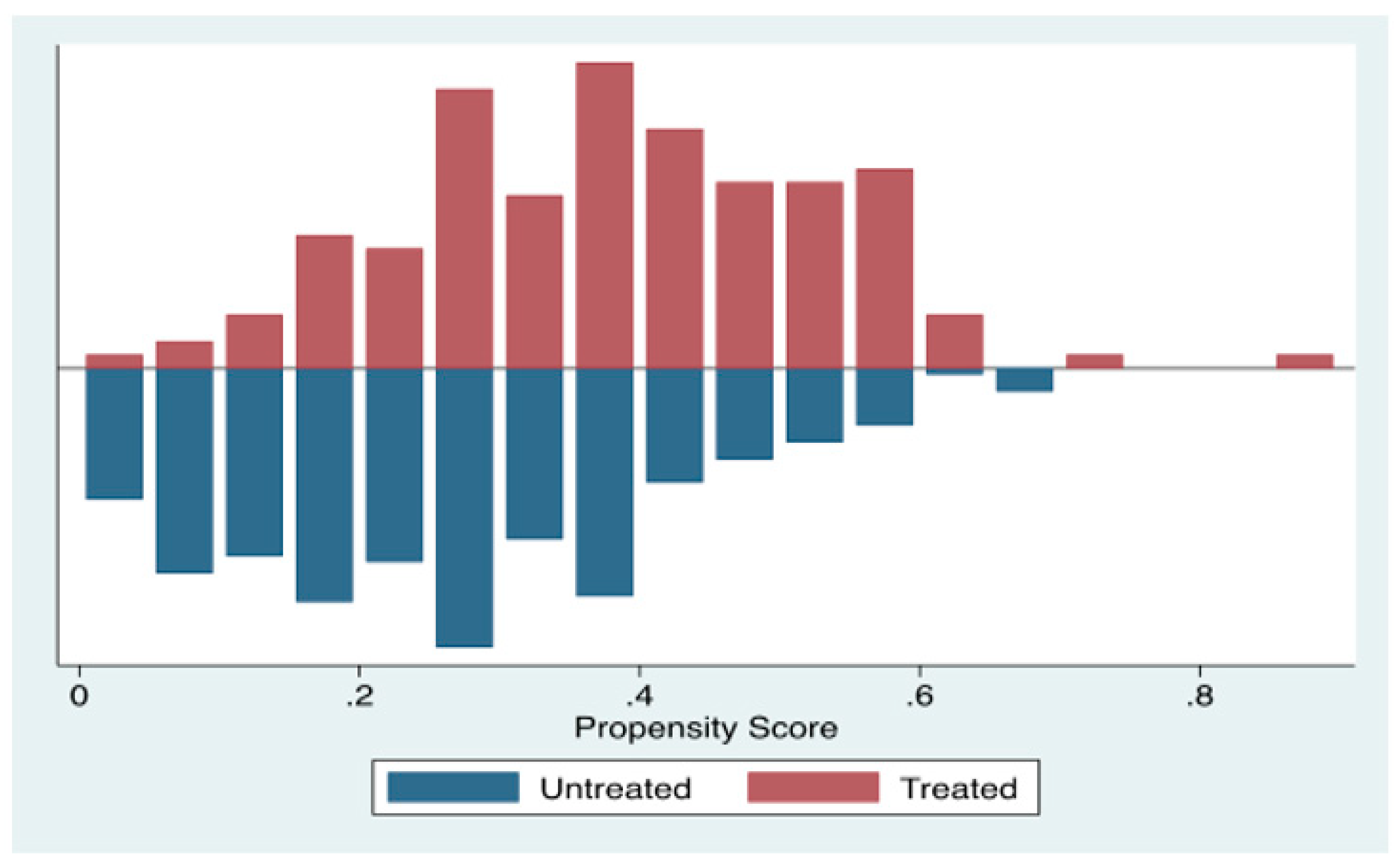
3.2. Propensity Score Matching (PSM)
4. Results and Discussion
4.1. Rainfall Variability in the Context of Climate Change
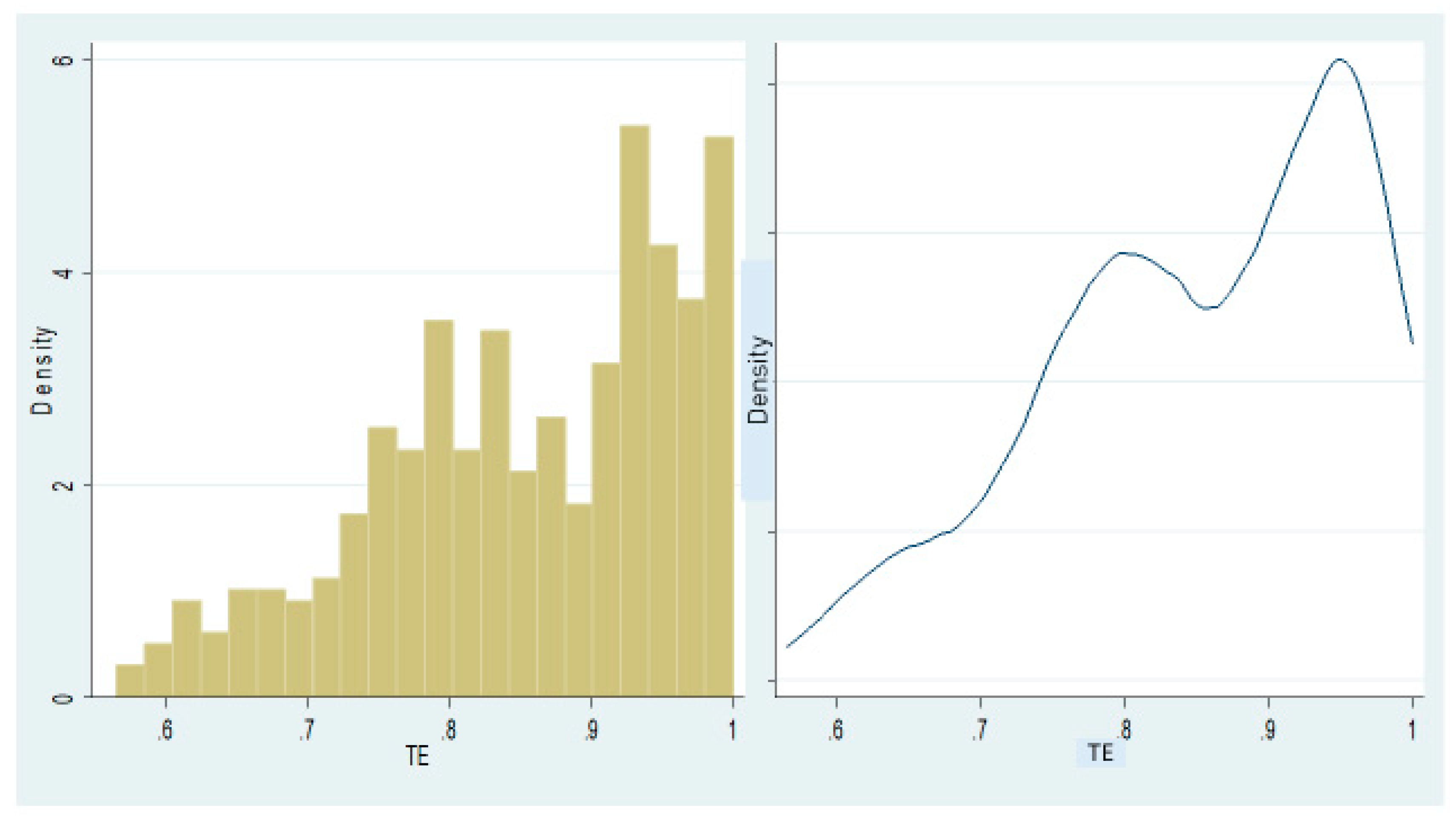
4.2. Data Envelopment Analysis (DEA)—TE of Groundnut Production
4.2.1. Summary Statistics of Output and Input Variables
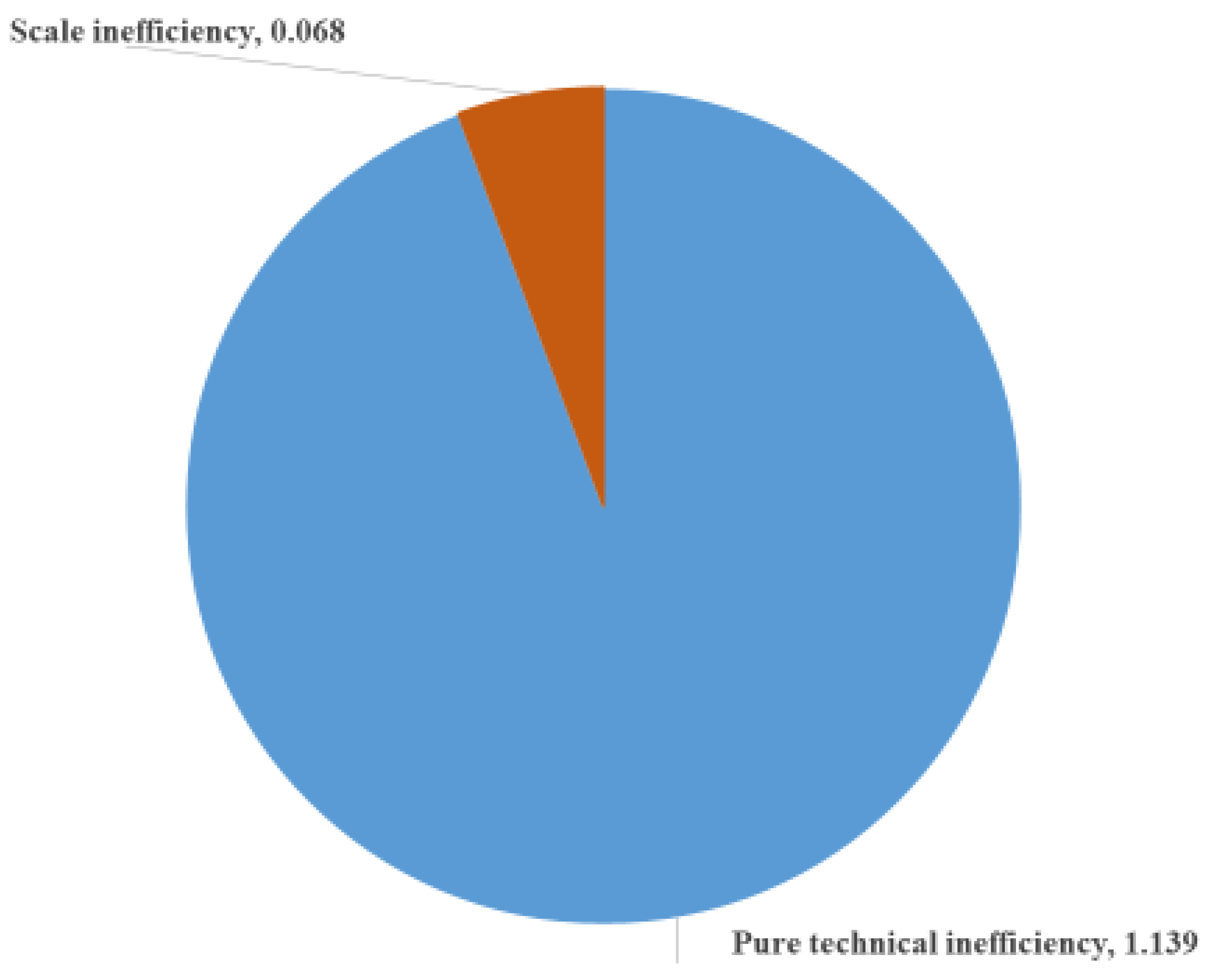
4.2.2. Overall TE, Pure TE and Scale Efficiency
- the splitting of overall TE measure produced estimates of 14 percent pure technical inefficiency and seven percent scale inefficiency (Figure 2);
- by eliminating scale inefficiency, the farms can increase their average overall TE from 0.790 to 0.861;
- the higher scale efficiency of 0.932 indicates that the majority of the groundnut farms are operating at or near to their optimal size;
- the overall technical inefficiency of groundnut farms by 21 percent implies that the farmers are not able to obtain optimal output from the given level of inputs available to them, and they are not utilizing the available inputs efficiently. The overall TE scores can be improved by adopting GAPs among groundnut farms.
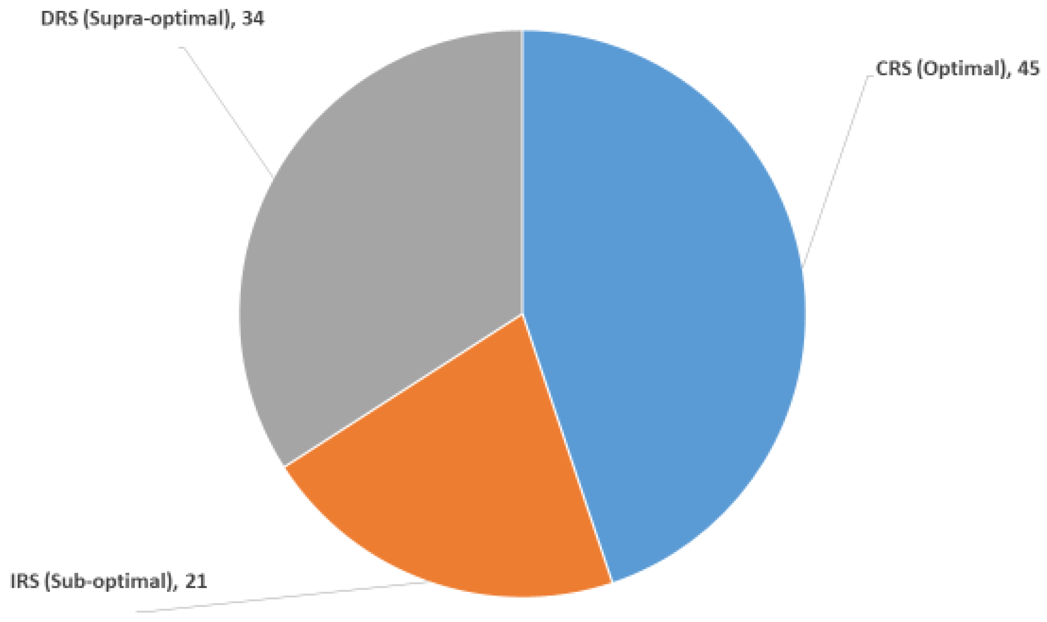
4.2.3. Scale of Operations in the Production Frontier
4.2.4. Input Slacks and Excess Input Usage
4.3. Impact of WBCIS Participation on TE of Groundnut Farms
5. Summary and Conclusions
- greater awareness and understanding about the WBCIS among farmers;
- better location of weather stations;
- coverage of more weather parameters or more perils;
- refining the design of the WBCIS (shorter claim settlement periods, greater transparency, and ease of enrollment);
- premium refund for successive no claims.
Author Contributions
Funding
Institutional Review Board Statement
Informed Consent Statement
Data Availability Statement
Acknowledgments
Conflicts of Interest
Appendix A

| Districts | Total Mandals | 1995–1996 | 1996–1997 | 1997–1998 | 1998–1999 | 1999–2000 | 2000–2001 | 2001–2002 | 2002–2003 | 2003–2004 | 2004–2005 | 2005–2006 | 2006–2007 | 2007–2008 | 2008–2009 | 2009–2010 | 2010–2011 | 2011–2012 | 2012–2013 | 2013–2014 | 2014–2015 | 2015–2016 | 2016–2017 | 2017–2018 |
|---|---|---|---|---|---|---|---|---|---|---|---|---|---|---|---|---|---|---|---|---|---|---|---|---|
| Srikakulam | 38 | 11 | 37 | 36 | 16 | 38 | 28 | 11 | 8 | 26 | 30 | 18 | 15 | |||||||||||
| Vizianagaram | 34 | 2 | 34 | 34 | 17 | 34 | 34 | 11 | 6 | 19 | 15 | 5 | 3 | 6 | 1 | |||||||||
| Visakhapatnam | 43 | 41 | 28 | 42 | 42 | 7 | 7 | 42 | 31 | |||||||||||||||
| East Godavari | 60 | 17 | 5 | 11 | 45 | 53 | 3 | 20 | 58 | 14 | ||||||||||||||
| West Godavari | 46 | 10 | 24 | 42 | 10 | 25 | 46 | 15 | ||||||||||||||||
| Krishna | 50 | 20 | 33 | 50 | 13 | 21 | 49 | 32 | 14 | |||||||||||||||
| Guntur | 57 | 37 | 7 | 53 | 57 | 1 | 24 | 55 | 41 | 4 | 4 | 26 | ||||||||||||
| Prakasam | 56 | 52 | 56 | 56 | 43 | 56 | 39 | 53 | 32 | 56 | 56 | 35 | 4 | 54 | 56 | 56 | 55 | |||||||
| Nellore | 46 | 43 | 36 | 46 | 18 | 46 | 46 | 40 | 40 | 46 | 9 | 9 | 2 | 7 | 33 | 27 | 15 | |||||||
| Chittoor | 66 | 66 | 32 | 65 | 45 | 65 | 65 | 42 | 56 | 37 | 66 | 49 | 28 | 33 | 20 | 40 | 66 | |||||||
| Kadapa | 51 | 37 | 50 | 51 | 5 | 51 | 51 | 32 | 49 | 33 | 51 | 51 | 43 | 16 | 42 | 55 | 32 | 27 | ||||||
| Ananthapuramu | 63 | 63 | 63 | 63 | 63 | 62 | 53 | 63 | 63 | 63 | 63 | 63 | 63 | 63 | 63 | 23 | ||||||||
| Kurnool | 54 | 54 | 53 | 52 | 54 | 31 | 46 | 30 | 49 | 54 | 36 | 48 | 51 | 36 | ||||||||||
| Total | 664 | 198 | 13 | 487 | 0 | 444 | 112 | 589 | 641 | 302 | 408 | 0 | 195 | 0 | 0 | 626 | 0 | 460 | 218 | 123 | 238 | 359 | 301 | 121 |
Appendix B
| Item | 2010–2011 | 2018–2019 |
|---|---|---|
| Net Area Sown (m. ha) | 1.10 (57.66) # | 0.88 (46.00) # |
| Gross Area Sown (m. ha) | 1.18 (61.60) # | 0.93 (48.41) # |
| Groundnut Area (m. ha) | 0.83 (70.74) * | 0.49 (53.02) * |
| Groundnut Production (m. tonnes) | 0.48 | 0.18 |
| Groundnut yield (kg/ha) | 577 | 360 |
| Groundnut irrigated area (m. ha) | 0.029 (17.47) ** | 0.031 (17.82) ** |
Appendix C
| Crops | 2013–2014 (kg/ha) | % Deviation Compared to State | 2014–2015 (kg/ha) | % Deviation Compared to State |
|---|---|---|---|---|
| Paddy | 2866.00 | −5.90 | 3933.00 | −42.21 |
| Jowar | 653.00 | −85.45 | 698.00 | −111.17 |
| Bajra | 673.00 | −124.67 | 1157.00 | 10.89 |
| Maize | 6105.00 | 12.91 | 2862.00 | −105.17 |
| Bengal gram | 781.00 | −57.87 | 248.00 | −104.84 |
| Groundnut | 577.00 | −55.63 | 360.00 | −71.39 |
References
- Agricultural Research Station (ARS); Ananthapuramu, Acharya NG Ranga Agricultural University (ANGRAU), Guntur, India. Personal communication, 2020.
- Nair, R. Crop Insurance in India: Changes and Challenges. Econ. Political Weekly 2010, 45, 19–22. [Google Scholar]
- Chetaille, A.; Lagrande, D. L’assurance Indicielle, une Réponse Face aux Risques Climatiques? Available online: https://www.inter-reseaux.org/wp-content/uploads/pdf_p20_21_Gret.pdf (accessed on 3 April 2021).
- Hazell, P.; Anderson, J.; Balzer, N.; Hastrup Clemmensen, A.; Hess, U.; Rispoli, F. L’assurance Basée sur un Indice Climatique: Potentiel D’expansion et de Durabilité pour l’agriculture et les Moyens de Subsistance en Milieu Rural. Available online: https://www.findevgateway.org/fr/paper/2010/01/lassurance-basee-sur-un-indice-climatique-potentiel-dexpansion-et-de-durabilite-pour (accessed on 2 February 2021).
- Burke, M.; de Janvry, A.; Quintero, J. Providing Index–Based Agricultural Insurance to Smallholders: Recent Progress and Future Promise; Documento de Trabajo. CEGA, University of California at Berkeley: Berkeley, CA, USA. 2010. Available online: http://siteresources.worldbank.org/EXTABCDE/Resources/7455676-1292528456380/7626791-1303141641402/7878676-1306270833789/Parallel-Session-5-Alain_de_Janvry.pdf (accessed on 4 April 2020).
- Heimfarth, L.E.; Musshoff, O. Weather index-based insurances for farmers in the North China Plain. Agric. Financ. Rev. 2011, 71, 218–239. [Google Scholar] [CrossRef]
- Clarke, D.J.; Clarke, D.; Mahul, O.; Rao, K.N.; Verma, N. Weather Based Crop Insurance in India. Available online: https://www.researchgate.net/publication/254073298_Weather_based_crop_insurance_in_India (accessed on 31 March 2021).
- Carter, M.; de Janvry, A.; Sadoulet, E.; Sarris, A. Index-Based Weather Insurance for Developing Countries: A Review of Evidence and a Set of Propositions for Up-Scaling. Available online: https://econpapers.repec.org/paper/fdiwpaper/1800.htm (accessed on 6 June 2021).
- Agricultural Statistics at a Glance 2019. Available online: https://eands.dacnet.nic.in/PDF/At%20a%20Glance%202019%20Eng.pdf (accessed on 1 May 2021).
- Narain, S.; Ghosh, P.; Saxena, N.; Parikh, J.; Soni, P. Climate Change—Perspectives from India. Available online: https://ruralindiaonline.org/en/library/resource/climate-change-perspectives-from-india/ (accessed on 3 June 2021).
- Handbook of Statistics, Ananthapuramu; Various Issues; Government of Andhra Pradesh: Ananthapuramu, India, 2019.
- Banker, R.D.; Charnes, A.; Cooper, W.W. Some Models for Estimating Technical and Scale Inefficiencies in Data Envelopment Analysis. Manag. Sci. 1984, 30, 1078–1092. [Google Scholar] [CrossRef]
- Charnes, A.; Cooper, W.W.; Rhodes, E. Measuring the efficiency of decision making units. Eur. J. Oper. Res. 1978, 2, 429–444. [Google Scholar] [CrossRef]
- Pradhan, A.K. Measuring Technical Efficiency in Rice Productivity Using Data Envelopment Analysis: A Study of Odisha. Int. J. Rural. Manag. 2018, 14, 1–21. [Google Scholar] [CrossRef]
- Greene, W.H. Econometric Analysis, 5th ed.; Prentice Hall: Upper Saddle River, NJ, USA, 2003. [Google Scholar]
- Verbeek, M. A Guide to Modern Econometrics, 3rd ed.; John Wiley & Sons: Chichester, UK, 2008. [Google Scholar]
- Willy, D.K.; Zhunusova, E.; Holm-Müller, K. Estimating the joint effect of multiple soil conservation practices: A case study of smallholder farmers in the Lake Naivasha basin, Kenya. Land Use Policy 2014, 39, 177–187. [Google Scholar] [CrossRef]
- Ali, A.; Erenstein, O. Assessing farmer use of climate change adaptation practices and impacts on food security and poverty in Pakistan. Clim. Risk Manag. 2017, 16, 183–194. [Google Scholar] [CrossRef]
- Rosenbaum, P.R. Overt Bias in Observational Studies. In Observational Studies; Springer: New York, NY, USA, 2002; pp. 71–104. [Google Scholar]
- Rosenbaum, P.R.; Rubin, D.B. The central role of the propensity score in observational studies for causal effects. Biometrika 1983, 70, 41–55. [Google Scholar] [CrossRef]
- Tipi, T.; Yildiz, N.; Nargeleçekenler, M.; Çetin, B. Measuring the technical efficiency and determinants of efficiency of rice (Oryza sativa) farms in Marmara region, Turkey. N. Z. J. Crop. Hortic. Sci. 2009, 37, 121–129. [Google Scholar] [CrossRef][Green Version]
- Simar, L.; Wilson, P.W. Two-stage DEA: Caveat emptor. J. Product. Anal. 2011, 36, 205–218. [Google Scholar] [CrossRef]
- Toma, P. Size and productivity: A conditional approach for Italian pharmaceutical sector. J. Prod. Anal. 2020, 54, 1–12. [Google Scholar] [CrossRef]
- Adebayo, O.; Bolarin, O.; Oyewale, A.; Kehinde, O. Impact of irrigation technology use on crop yield, crop income and household food security in Nigeria: A treatment effect approach. AIMS Agric. Food 2018, 3, 154–171. [Google Scholar] [CrossRef]
- Becker, S.O.; Caliendo, M. Sensitivity Analysis for Average Treatment Effects. Stata J. 2007, 7, 71–83. [Google Scholar] [CrossRef]


| Item | Jan | Feb | Mar | Apr | May | June | July | Aug | Sept | Oct | Nov | Dec | Annual Rf | JF | MAM | JJAS | OND |
|---|---|---|---|---|---|---|---|---|---|---|---|---|---|---|---|---|---|
| 1926–1975 | |||||||||||||||||
| Mean | 0.940 | 2.820 | 3.700 | 15.600 | 54.900 | 56.160 | 55.460 | 77.700 | 131.260 | 115.180 | 33.440 | 9.280 | 556.440 | 3.760 | 74.200 | 320.580 | 157.900 |
| SD | 3.347 | 5.944 | 9.498 | 19.736 | 39.688 | 42.160 | 45.092 | 91.302 | 82.647 | 92.307 | 43.682 | 17.948 | 141.997 | 6.859 | 45.326 | 115.945 | 101.834 |
| CV(%) | 356.032 | 210.790 | 256.706 | 126.513 | 72.292 | 75.072 | 81.306 | 117.505 | 62.964 | 80.142 | 130.627 | 193.403 | 25.519 | 182.415 | 61.086 | 36.167 | 64.493 |
| % Contribution to Annual Rainfall (1926–1975) | 0.17 | 0.51 | 0.66 | 2.80 | 9.87 | 10.09 | 9.97 | 13.96 | 23.59 | 20.70 | 6.01 | 1.67 | 100.00 | 0.68 | 13.33 | 57.61 | 28.38 |
| 1976–2019 | |||||||||||||||||
| Mean | 1.536 | 2.257 | 6.914 | 15.489 | 46.627 | 54.332 | 56.455 | 76.977 | 123.520 | 96.875 | 36.934 | 6.852 | 524.768 | 3.793 | 69.030 | 311.284 | 140.661 |
| SD | 3.133 | 6.107 | 14.267 | 17.442 | 36.777 | 37.838 | 48.720 | 53.199 | 74.184 | 55.623 | 45.261 | 10.427 | 146.882 | 6.562 | 44.871 | 118.741 | 65.713 |
| CV(%) | 203.891 | 270.614 | 206.360 | 112.613 | 78.874 | 69.642 | 86.300 | 69.110 | 60.058 | 57.417 | 122.545 | 152.167 | 27.990 | 173.004 | 65.002 | 38.145 | 46.717 |
| % Contribution to Annual Rainfall (1976–2019) | 0.29 | 0.43 | 1.32 | 2.95 | 8.89 | 10.35 | 10.76 | 14.67 | 23.54 | 18.46 | 7.04 | 1.31 | 100.00 | 0.72 | 13.15 | 59.32 | 26.80 |
| 1926–2019 | |||||||||||||||||
| Mean | 1.219 | 2.556 | 5.204 | 15.548 | 51.028 | 55.304 | 55.926 | 77.362 | 127.637 | 106.612 | 35.076 | 8.144 | 541.615 | 3.776 | 71.780 | 316.229 | 149.831 |
| SD | 3.245 | 5.995 | 12.010 | 18.598 | 38.373 | 39.992 | 46.573 | 75.503 | 78.476 | 77.487 | 44.222 | 14.882 | 144.400 | 6.686 | 44.945 | 116.721 | 86.806 |
| CV(%) | 266.141 | 234.519 | 230.776 | 119.619 | 75.201 | 72.312 | 83.277 | 97.598 | 61.484 | 72.681 | 126.077 | 182.744 | 26.661 | 177.079 | 62.615 | 36.910 | 57.936 |
| % Contribution to Annual Rainfall (1926–2019) | 0.23 | 0.47 | 0.96 | 2.87 | 9.42 | 10.21 | 10.33 | 14.28 | 23.57 | 19.68 | 6.48 | 1.50 | 100.00 | 0.70 | 13.25 | 58.39 | 27.66 |
| 1990–2019 (Climate Change Period) | |||||||||||||||||
| Mean | 1.920 | 2.443 | 8.017 | 17.387 | 48.570 | 58.953 | 53.037 | 78.917 | 113.150 | 110.623 | 32.737 | 5.920 | 531.673 | 4.363 | 73.973 | 304.057 | 149.280 |
| SD | 3.390 | 6.515 | 16.771 | 18.481 | 28.679 | 36.673 | 36.874 | 43.551 | 64.524 | 52.093 | 33.933 | 10.508 | 128.695 | 6.847 | 38.347 | 104.297 | 54.697 |
| CV(%) | 176.546 | 266.638 | 209.202 | 106.293 | 59.047 | 62.206 | 69.526 | 55.186 | 57.025 | 47.091 | 103.655 | 177.495 | 24.206 | 156.929 | 51.839 | 34.302 | 36.641 |
| % Contribution to Annual Rainfall (1990–2019) | 0.36 | 0.46 | 1.51 | 3.27 | 9.14 | 11.09 | 9.98 | 14.84 | 21.28 | 20.81 | 6.16 | 1.11 | 100 | 0.82 | 13.91 | 57.19 | 28.08 |
| Item | Minimum | Maximum | Mean | SD | CV |
|---|---|---|---|---|---|
| Groundnut production (kg) | 1462 | 3525 | 1965.63 | 174.81 | 8.8933 |
| Fertilizer Use (NPK) (kg/ha) | 350 | 455 | 410.58 | 89.62 | 21.8276 |
| Seed rate (kg/ha) | 145 | 170 | 154.27 | 56.97 | 36.9288 |
| Gypsum (kg/ha) | 340 | 650 | 580.16 | 192.57 | 33.1926 |
| Organic manure (t/ha) | 2.00 | 12.00 | 9.35 | 4.91 | 52.5134 |
| Efficiency Level | Overall TE | Pure TE | Scale Efficiency | |||
|---|---|---|---|---|---|---|
| No. of Farms | Percent | No. of Farms | Percent | No. of Farms | Percent | |
| ≤0.60 | 9 | 1.89 | 8 | 1.68 | 2 | 0.42 |
| 0.61–0.70 | 23 | 4.83 | 20 | 4.20 | 11 | 2.31 |
| 0.71–0.80 | 62 | 13.03 | 54 | 11.34 | 23 | 4.83 |
| 0.81–0.90 | 123 | 25.84 | 141 | 27.52 | 142 | 29.83 |
| 0.91–0.99 | 192 | 40.34 | 190 | 39.92 | 210 | 44.12 |
| 1.00 | 67 | 14.08 | 73 | 15.34 | 88 | 18.49 |
| Total | 476 | 100.00 | 476 | 100.00 | 476 | 100 |
| Minimum | 0.582 | 0.591 | 0.638 | |||
| Maximum | 1.000 | 1.000 | 1.000 | |||
| Mean | 0.790 | 0.861 | 0.932 | |||
| Median | 0.782 | 0.903 | 0.989 | |||
| SD | 0.19 | 0.17 | 0.09 | |||
| Characteristics | No. of Farms | Mean Farm Size (ha) | Mean Output (Tonnes) |
|---|---|---|---|
| CRS (Optimal) | 213 (44.75) | 1.73 | 3.61 |
| DRS (Supra-optimal) | 162 (34.03) | 1.58 | 3.18 |
| IRS (Sub-optimal) | 101 (21.22) | 1.23 | 2.69 |
| Inputs | No. of Farms | % of Total Farms | Mean Input Slack | Mean Input Used | Excess Input Use in Percent |
|---|---|---|---|---|---|
| Fertilizer Use (NPK) (kg/ha) | 97 | 20.38 | 16.58 | 410.58 | 4.04 |
| Seed rate (kg/ha) | 81 | 17.02 | 12.59 | 154.27 | 8.16 |
| Gypsum (kg/ha) | 52 | 10.92 | 9.12 | 580.16 | 1.57 |
| Organic manure (t/ha) | 29 | 6.09 | 0.96 | 9.35 | 10.27 |
| Percentiles | Smallest | |||
|---|---|---|---|---|
| 1% | 0.0516 | 0.0419 | ||
| 5% | 0.0832 | 0.0429 | ||
| 10% | 0.1100 | 0.0479 | Obs | 455 |
| 25% | 0.1946 | 0.0506 | ||
| 50% | 0.2995 | Mean | 0.3117 | |
| Largest | Std. Dev. | 0.1507 | ||
| 75% | 0.4094 | 0.6633 | ||
| 90% | 0.5222 | 0.6633 | Variance | 0.0227 |
| 95% | 0.5723 | 0.7085 | Skewness | 0.2989 |
| 99% | 0.6557 | 0.8568 | Kurtosis | 2.525 |
| Variable | Unmatched/ Matched | Mean | % Bias | % Reduction in Bias [100(1-(BiasAM/BiasBM))] | ‘t’ test | ||
|---|---|---|---|---|---|---|---|
| Treated | Untreated | tcal | p > |t| | ||||
| AGE | Unmatched | 52.407 | 51.169 | 10.8 | 1.13 | 0.260 | |
| Matched | 52.407 | 52.073 | 2.9 | 73.1 | 0.25 | 0.803 | |
| LHS | Unmatched | 3.6567 | 3.1271 | 55.7 | 5.51 *** | 0.000 | |
| Matched | 3.6567 | 3.6267 | 3.2 | 94.3 | 0.31 | 0.759 | |
| EDU | Unmatched | 4.2267 | 4.2457 | −0.4 | −0.04 | 0.967 | |
| Matched | 4.2267 | 4.1467 | 1.6 | −320.0 | 0.13 | 0.893 | |
| GAPs | Unmatched | 0.58 | 0.843 | −40.2 | −3.81 *** | 0.000 | |
| Matched | 0.58 | 0.66 | −12.2 | 69.6 | −1.18 | 0.238 | |
| FE | Unmatched | 30.687 | 26.331 | 38.3 | 3.98 *** | 0.000 | |
| Matched | 30.687 | 31.2 | −4.5 | 88.2 | −0.38 | 0.701 | |
| TIME | Unmatched | 1.8733 | 1.8343 | 5.6 | 0.55 | 0.579 | |
| Matched | 1.8733 | 1.76 | 16.3 | −190.2 | 1.47 | 0.141 | |
| Outcome | Sample | Treated | Untreated | Difference | SE | t-Stat |
|---|---|---|---|---|---|---|
| NNM | Unmatched | 0.8850 | 0.7367 | 0.1483 *** | 0.0092 | 16.07 |
| ATT | 0.8850 | 0.7294 | 0.1557 *** | 0.0131 | 11.91 | |
| ATU | 0.7367 | 0.8925 | 0.1559 | |||
| ATE | 0.1558 | |||||
| KBM | Unmatched | 0.8850 | 0.7367 | 0.1483 *** | 0.0092 | 16.07 |
| ATT | 0.8848 | 0.7308 | 0.1539 *** | 0.0094 | 16.4 | |
| ATU | 0.7367 | 0.8903 | 0.1536 | |||
| ATE | 0.1537 | |||||
| RM | Unmatched | 0.8850 | 0.7367 | 0.1483 *** | 0.0092 | 16.07 |
| ATT | 0.8860 | 0.7313 | 0.1548 *** | 0.0091 | 17.13 | |
| ATU | 0.7344 | 0.8894 | 0.1549 | |||
| ATE | 0.1549 |
| Indicators | Before Matching | After Matching |
|---|---|---|
| Pseudo-R2 | 0.105 | 0.016 |
| LR chi2 | 64.15 | 6.68 |
| P > chi2 | 0.000 | 0.351 |
| Mean Absolute Bias | 25.2 | 6.8 |
| Med Bias | 24.5 | 13.8 |
| Outcome Variable | Gamma * | Significance Level | Hodges–Lehmann Point Estimate | Confidence Interval (95%) | |||
|---|---|---|---|---|---|---|---|
| Upper Bound | Lower Bound | Upper Bound | Lower Bound | Upper Bound | Lower Bound | ||
| TE | Γ = 1 | 0 | 0 | 0.1615 | 0.1615 | 0.14 | 0.1835 |
| Γ = 2 | 2.70 × 10⁻¹¹ | 0 | 0.1225 | 0.202 | 0.098 | 0.2245 | |
| Γ = 3 | 1.70 × 10⁻⁷ | 0 | 0.099 | 0.2235 | 0.0725 | 0.2465 | |
| Γ = 4 | 0.000014 | 0 | 0.083 | 0.2375 | 0.055 | 0.261 | |
| Γ = 5 | 0.000195 | 0 | 0.0715 | 0.2475 | 0.0415 | 0.2715 | |
Publisher’s Note: MDPI stays neutral with regard to jurisdictional claims in published maps and institutional affiliations. |
© 2021 by the authors. Licensee MDPI, Basel, Switzerland. This article is an open access article distributed under the terms and conditions of the Creative Commons Attribution (CC BY) license (https://creativecommons.org/licenses/by/4.0/).
Share and Cite
Kumar, K.N.R.; Babu, S.C. Can a Weather-Based Crop Insurance Scheme Increase the Technical Efficiency of Smallholders? A Case Study of Groundnut Farmers in India. Sustainability 2021, 13, 9327. https://doi.org/10.3390/su13169327
Kumar KNR, Babu SC. Can a Weather-Based Crop Insurance Scheme Increase the Technical Efficiency of Smallholders? A Case Study of Groundnut Farmers in India. Sustainability. 2021; 13(16):9327. https://doi.org/10.3390/su13169327
Chicago/Turabian StyleKumar, K. Nirmal Ravi, and Suresh Chandra Babu. 2021. "Can a Weather-Based Crop Insurance Scheme Increase the Technical Efficiency of Smallholders? A Case Study of Groundnut Farmers in India" Sustainability 13, no. 16: 9327. https://doi.org/10.3390/su13169327
APA StyleKumar, K. N. R., & Babu, S. C. (2021). Can a Weather-Based Crop Insurance Scheme Increase the Technical Efficiency of Smallholders? A Case Study of Groundnut Farmers in India. Sustainability, 13(16), 9327. https://doi.org/10.3390/su13169327