Article

Sustainable Construction and Financing—Asset-Backed Securitization of Expressway’s Usufruct with Redeemable Rights

1
School of Economics and Management, Beijing Jiaotong University, Beijing 100044, China
2
Department of Asian and International Studies, City University of Hong Kong, Hongkong 999077, China
3
Architecture and the Built Environment, Delft University of Technology, 2600 Delft, The Netherlands
*
Authors to whom correspondence should be addressed.
Sustainability 2021, 13(16), 9113; https://doi.org/10.3390/su13169113
Submission received: 11 July 2021 / Revised: 8 August 2021 / Accepted: 12 August 2021 / Published: 14 August 2021

Abstract

:
Asset-backed securitization will greatly promote the sustainability of infrastructure construction and financing. However, there are quite limited researches conducted in this field. Given the project characteristics of infrastructure project securities, this paper proposes the issuance steps of redeemable asset-backed notes (ABN) based on the infrastructure project’s usufruct as the basic asset. Taking the expressway franchise as an example, the issuing scale and coupon rate of the redeemable ABN are determined by the expected cash flow of the expressway, the term structure of random interest rates, and the option-adjusted spread (OAS). In addition, this research analyzes the duration, convexity, and OAS.

1. Introduction

The characteristics of infrastructure projects are low risk, stable returns, and steady operation of the main body. Compared with other investment products, the credit risk of asset-backed securities tends to be low while its yields are high. These infrastructure asset securitization products attract corporations and individual investors, pension funds, social security funds, etc., to invest monetary stock because of its stable returns and long maturities. The central banks of the two economic powerhouses, the United States and Japan, successively bought asset securitization products such as mortgage-backed securities (MBS) and Real Estate Investment Trusts (REITs) in open market operations, and used them as asset backing to release the base currency after the financial crisis in 2008. As of 2019, the United States has invested USD 190,206 million in securitized REITs products in the infrastructure sector.
Local governments in China are not allowed to secure bank loans. However, a massive influx of funding is needed to construct the public rental housing, renovate the shantytown, construct the roads, and develop public transportation and other infrastructures [1]. Local governments use government finances as a guarantee to borrow money from banks through setting up local government financial vehicles (LGFVs). However, some LGFVs “cannot make ends meet”, causing domestic and foreign concerns about the local debt problems of China [2]. To achieve sustainable development, local governments could ease their debt burden by issuing infrastructure asset securitization products. The local government could sell the expected usufruct of assets to Special Purpose Vehicle (SPV), and the SPV will issue asset-backed securities for financing. Investing in funds could assist in recovering the investment costs in advance and ease the debt burden of the local government. On the one hand, Chinese local governments demand to issue asset securitization products for financing. On the other hand, they also need the right to redeem bonds. Affected by the continued decline of the interest rates, a total of 96 LGFVs on the open market in 2017 proposed to redeem their issued bonds, involving 121 bonds (collected from the WIND database). In this case, the launch of infrastructure asset securitization products with redemption rights becomes particularly necessary.
In the traditional analysis of fixed-income products, scholars have used the yield to maturity and the spread based on it as important indicators to analyze the risk-return relationship of fixed-income products. However, with the intensification of interest rate fluctuations and the vigorous development of weighted bonds, the inherent shortcomings of the yield to maturity and its spread indicators have become increasingly prominent. First, the yield to maturity assumes that the spot interest rates at all moments in the future are equal, which is different from the reality of multiple shapes of the term structure of interest rates in practice. Second, due to the possibility of the inclusion of the options of the issuer (such as redeemable or prepayable bonds) or the options of investors (such as the callable bond), future interest rate fluctuations may change the cash flow of future bonds (bonds may repay the principal part or all in advance). The yield to maturity does not consider this uncertainty. If the bond contains highly complex options, the yield to maturity will be more inaccurate. Regarding the uncertain impact of various transaction structures on the term structure and the risks of fixed income products, entropy indicators have become an important tool in the field of asset pricing gradually. Filipović and Willems [3] identified the density function through the entropy method and priced the options of dividend stocks and the interest rate–dividend hybrid derivatives, which contributed to the analysis of yield with uncertain distribution. Sheraz et al. [4] believed that in many cases, no arbitrage risk measurement was difficult to be realized through using numerical method, and the minimum entropy method provided a new idea for the determination of risk neutral measurement. Based on HJ pricing kernel, Rojo-Suárez and Alonso Conde [5] divided the core of asset pricing into two parts, the relative entropy of the pricing kernel and the relative entropy related to asset pricing. Liao et al. [6] calculated the yield volatility of each sub-market of Chinese bond market through an auto-regressive model, and further got the volatility spillover effect between each sub-market of bonds. In the research, Liao found that the inter-bank market was the core of Chinese bond market, and believed that structural entropy was an important factor to influence the risk of the bond market. For the local governments of China, although the entropy methods have attracted lots of attentions in the field of asset pricing research, there is still a long way to go for practical application. Therefore, with the increasing complexity of option-embedded bonds in the market, investors have begun to widely use a yield indicator that comprehensively considers the term structure and the impact of embedded options, Option-Adjusted Spread (OAS). It is used to replace the yield to maturity to analyze the pricing and risk management of option-embedded bonds. For the MBS, the OAS analysis method has become one of the most important pricing and analysis management models.
Many asset-backed securitization products in the infrastructure sector are issued in the form of asset-backed notes (ABN), but there have been limited studies on ABN pricing. Therefore, this paper focuses on the pricing of the redeemable ABN. Taking the pricing of asset securitization of expressway usufruct as an example, this paper draws on the pricing method of securitization products which are similar to the ABN structure. It combines the specific characteristics of the expressway usufruct asset pool and uses the option-adjusted spread method to design a redeemable ABN pricing model.
The innovations of this research are two-fold: (1) By combining the Kalman filtering method with the two-factor Vasicek model to simulate the term structure of stochastic interest rates, as well as by calculating the OAS, proposing the pricing steps of redeemable ABN, and carrying out the empirical simulation, this paper enriches the pricing theory of asset securitization products and provides a theoretical basis for determining reasonable prices when ABN products are traded in REITs in the future; (2) By designing redeemable asset-backed securitization products with infrastructure income rights, this research proposes a more flexible long-term and sustainable financing method for infrastructure services.

2. Literature Review of Asset-Backed Securitization Product Pricing

The pricing of asset-backed securitization products has been mainly used to analyze the expected cash flow that the asset pool will generate in the future. The present value of the asset-backed securities has obtained by predicting the future interest rate path and discounting the expected cash flow [7]. Jacob et al. [8] defined two independent stochastic processes for the risk-free interest rate and the net operating income of the underlying assets, which extends the default mortgage pricing model. This research has also set prices for commercial mortgage-backed securities (CMBS). Sharp et al. [9] proposed a singular perturbation theoretical model based on the random house price-interest rate model. This allowed the value of the mortgage loan to be estimated in a very simple analytical solution form, which reduced the calculation time. Liu et al. [10] believed that the CMBS default rate has a great relationship with the extreme events that occurred in the transaction process and the correlation of default. Based on previous studies, Liu et al. proposed a pricing method based on the copula model to price CMBS bonds. Hürlimann [11] used a simplified binary tree estimation model to price fixed-rate prepayment mortgages, which tend to be more accurate than analytical solutions. Qian et al. [12] supposed that the prepayment function obeyed the stochastic process B i = e 0 t λ s d s , and the interest rate r t obeyed the CIR process, in which the prepayment rate λ s is negatively correlated with the interest rate r t . By solving the PDE method, this research introduced the precise formula of the value of the passed MBS and the semi-analytical solution form of the value of the CMO (secured mortgage bond). Fan et al. [13] pointed out that default was a Poisson jumping process determined by the information function of mortgage credit rating, and used higher-dimensional Brownian motion to capture systemic risks and idiosyncratic risks. Fermanian [14] found that it was possible to directly model the loss process and amortization process of the investment portfolio based on the “top-down” path of the pricing of bond graded products such as CMO (Collateralized Mortgage Obligation) and CDO (Collateralized Debt Obligation).
Hayre [15] proposed that the basic idea of the OAS model was to describe the price of bonds with built-in options (such as mortgage-backed securities with early repayment characteristics) under different interest rate backgrounds. These interest rate backgrounds included all possible conditions of interest rates over a period. On each interest rate branch, there was a series of cash flows corresponding to different interest payments. Green [16] proposed the general steps for calculating OAS. The first step was to determine the term structure of the benchmark interest rate of the current date from the market price of non-weighted bonds on that day. They then constructed a term structure of interest rate volatility based on historical information or the implied volatility of the corresponding interest rate option (if there is a corresponding options market). The second step was to use an appropriate stochastic process, such as the Black–Derman–Toy Model (BDT), to describe the dynamic changes of interest rates and adopt simulation methods that generated various possible paths for future interest rates changes. Since the term structure of the benchmark interest rate and the term structure of interest rate volatility were used as input variables in the simulation process, the entire simulation process had the nature of no-arbitrage. The third step was to follow each possible way to adjust the path of interest rate changes and calculate future cash flows under different scenarios according to the nature of the options contained in the bond. This method was similar to the simulation of American options. It was necessary to determine whether to execute the option to determine the cash flow for each moment of the cash flow. The fourth step was to calculate the OAS by discounting the future cash flow. Dong et al. [17] used the Schwartz and Torous pricing models and took Jianyuan 2007-1RMBS as the research object to simulate the term structure of interest rates under the BDT interest rate model. They priced the MBS by combing the option to adjust the spread OAS.
Generally, it can be found that the current research on asset-backed securitization focuses mostly on MBS and RMBS, with quite limited research on ABN securities, which was widely used in the field of infrastructure. ABN was also a type of fixed-income securities, and its pricing was similar to the pricing ideas of other asset-backed securities, that is, discounting future cash flows to the point of pricing. In summary, combining the cash flow characteristics of expressway toll rights, this article proposes a pricing idea of redeemable ABN with expressway toll rights as the basic asset.

3. Issuance Scale and Coupon Rate Pricing of Redeemable ABN

3.1. The Issuance Steps of a Redeemable ABN

Assuming that ABN with expressway toll rights as the basic asset generates cash flow annually, with N years duration and paying the interest once a year, the bond issuer could redeem the bond at the agreed price K at the agreed time. This research focused on how to determine the issuance scale and coupon rate of a redeemable ABN based on the expected value of highway tolls and the term structure of interest rates. It could be described mainly as the following six steps:
The first step was to predict the net cash flow of N C F t in each period in the future. Then, we analyzed the influencing factors of expressway tolls. We calculated the cash flow of the expressway in each period in the next N years and obtains the expected net cash flow N C F t of the expressway income right in year t according to the historical data of monthly tolls of expressways in nearby locations and regional economic development.
The second step was to fit the yield to maturity curve:
(1) Fitting the yield curve of treasury bonds and calculating OAS
We found the relevant data of the traded Treasury bonds in a certain time interval before the pricing point, including the name of the bond, the maturity time, the coupon rate, the net price, the full price, the remaining maturity, etc., and used the Nelson and Siegel (NS) or Svensson (SV) model to fit the term structure curve of the static interest rate of the national debt in this time interval.
The term structure of interest rates was calculated based on real market data. Using the Kalman filter method and the two-factor Vasicek [18] model, we generated M interest rate paths. For the selection of an interest rate model, Vázquez-Vázquez et al. [19] used a single-factor Vasicek model to simulate short-term risk-free interest rates. Pelizzari and Paolo [20] used a two-factor combination model including the Vasicek model and the Cox–Ingersoll–Ross model to fit the term structure of inflation and interest rates. The Cox–Ingersoll–Ross model has the limitation of adapting negative interest rates. In order to implement the monetization of fiscal deficit, the central banks may implement negative nominal interest rates. For example, many central banks such as the European Central Bank and the Bank of Japan are implementing negative nominal deposit interest rates. Given this situation, we believe that the two-factor Vasicek model was more appropriate for the current interest rate environment.
The treasury bond price on the i interest rate path was determined by the following formula.
B i ( t ) = t M a t u r i t y 1 C o u p o n t e x p [ t 0 t ( f ( t ) i ) d t ] + F a c e V a l u e   e x p [ M a t u r i t y 0 M a t u r i t y ( f ( t ) i ) d t ]
The cash flow of early redemption corresponding to each interest rate path needed to be determined if the national debt is redeemable. The method used here referred to the Longstaff’s [21] American option pricing model. Since it was impossible for local governments to redeem financing products as flexibly as American options, we have simplified the model to make it more practical. Assumed that at the redeemable time point, when the bond price B i ( t ) < K , bond redemption occurs. At the time of redemption ( R e p o ), the income of the bond purchaser was K , the cash flow after the redemption time was cleared to zero, and the theoretical price B i of the national bond with rights on the i -th interest rate path was obtained.
B i = t M a t u r i t y 1 C o u p o n t e x p [ t 0 t ( f ( t ) i ) d t ] + K   e x p [ M a t u r i t y 0 R e p o ( f ( t ) i ) d t ]
We got the theoretical price B of the national debt with rights by calculating the average price of M paths. Then, the option-adjusted spread superimposed on the term structure of the benchmark interest rate of the treasury bond (obtained from the average of the M interest rate paths) was changed, so to make the theoretical price of the treasury bond was equal to the face value of the treasury bond with rights, thereby obtaining the option adjusted spread (OAS).
B = t M a t u r i t y 1 C o u p o n t i e x p [ t 0 t ( f ( t ) + O A S ) d t ] + F a c e V a l u e   e x p [ M a t u r i t y 0 M a t u r i t y ( f ( t ) + O A S ) d t ]
(2) Calculating the credit spreads. According to the overall credit rating results of the asset pool, we obtained data on corporate bonds at the time of pricing, including bond name, bond rating, maturity time, coupon rate, net price, full price, accrued interest, and remaining Term, etc., and calculated the credit spread (Z-spread);
(3) We superimposed the credit spreads and the option adjustment spreads on the benchmark interest rate curve of treasury bonds to obtain the yield-to-maturity curve of the corresponding credit-grade bonds, and we got the yield-to-maturity r t in year t .
The third step was to determine the issuance scale of bonds of different grades. According to the credit rating results of the underlying assets, the expressway income right ABN was divided into A-level bonds, B-level bonds,..., and Z-level bonds. Among them, Grade A bonds had the highest credit rating, while Grade Z bonds had the lowest credit rating.
According to the expected annual net cash flow N C F t in the next N years and the yield to maturity r t of each grade, the discounted cash flow (DCF) pricing method was used to obtain the present value NAV of the underlying asset.
According to the NAV value, the author determined the bond issuance scale.
N A V = t = 1 N N C F t   e x p ( r t t )
This article draws mainly on Fermanian’s (2013) grading method of sequential bond repayment.
According to Formula (4), and the expected cash flow of different grades of bonds and the term structure of interest rates, the fund size of bonds other than Z grades was determined. Z-rated bonds were usually held by the issuer of asset-backed securities and provide guarantees for other higher credit-rated bonds. Before the maturity of all higher-level bonds, no principal and interest would be paid to Z-level bonds. Z-level bonds were the distribution of the remaining funds in the asset pool. Therefore, the capital scale of Z-level bonds was the total capital scale minus the remaining part of the capital scale of other bonds.
The fifth step was to determine the coupon rates of bonds of different grades. It is assumed that, except for the Z bonds, all other bonds were issued at par. If the face value of the bond is CNY 100, and the interest was paid once a year, letting the maturity date of the bond be N and the coupon rate be C R , the yield to maturity r t in year t could be determined according to the interest rate term structure of the bond with the same credit rating. Then the bond coupon rate CR could be obtained by Formula (5).
100 = t = 1 N 100 × C R × e x p ( r t t ) + 100 × e x p ( r N N )
The sixth step was to analyze the interest rate risk of ABN products. ABN was an interest rate derivative product and had interest rate risk which was similar to other fixed-income securities. Interest rate risk referred to the risk that mortgage lending institutions or securities investors suffer losses due to changes in interest rates. Because of the stable future earnings of expressways and low default rates, interest rate risk is the main risk of ABN. This article used modified duration and convexity to measure the sensitivity of fixed income securities to interest rates.
According to Fabozzi [22], the modified duration MD and convexity C were defined as follows:
M D = p p + 2 P 0 y
C = p + p + p 0 2 P 0 ( y ) 2
p 0 was the current price of ABN, y was the fluctuation of the yield to maturity, p + was the price level of the security when the yield to maturity increases by y , and p represents the price level of the security when the yield to maturity decreases by y .

3.2. NS Model and SV Model

Since the two factors of the Vasicek model were not observable, the Kalman filter method was mainly used for parameter estimation. However, this method required observations of spot interest rates as data. Therefore, the static estimation method of the term structure of interest rates should be used to generate spot interest rate data. This paper used the Nelson–Siegel [23] model as the static estimation method. Section 3.2 and Section 3.3 briefly introduce the Nelson–Siegel model and the related theories of Kalman filtering.
Nelson and Siegel (1987) proposed the NS model, which used parameters to represent the instantaneous forward interest rate function f ( t ) .
f ( t ) = β 0 + β 1   e x p ( t τ 1 ) + β 2 ( t τ 1 ) e x p ( t τ 1 )
t represented the remaining maturity of the bond, and τ 1 was a positive time constant. According to the relationship between the spot interest rate R ( t ) and the forward interest rate f ( t ) , the function of R ( t ) to the remaining life t was:
R ( t ) = β 0 + β 1 [ 1 e x p ( t τ 1 ) t τ 1 ] + β 2 [ 1 e x p ( t τ 1 ) t τ 1 e x p ( t τ 1 ) ]
The principle of determining the parameters to be estimated in the model was to minimize the error between the theoretical price of the bond and the actual price of the day, that was, to achieve:
m i n i = 1 n ( P i P i ) 2 n
where n was the sample bond capacity, P i was the actual price of the i -th bond, and P i was the theoretical price of the bond. The theoretical bond price formula was:
P i = t F t i   e x p [ t R ( 0 , t ) ]
where F t i was the cash flow generated by bond i at time t . The theoretical price of the bond was obtained by adding the discounted value of the cash flows in each period. It was still assumed that the current period was the starting point of time 0.
The SV model was an improvement of the NS model by Svensson [24]. Two parameters β 3 and τ 2 were added, which solved the problem that the NS model could not reflect the multi-peak interest rate curve and improve the model’s ability to fit complex interest rate curves. In the SV model, the functional form of the instantaneous forward interest rate function f ( t ) and the spot interest rate R ( t ) were as follows:
f ( t ) = β 0 + β 1 e x p ( t τ 1 ) + β 2 ( t τ 1 ) e x p ( t τ 1 ) + β 3 ( t τ 2 ) e x p ( t τ 2 )
R ( t ) = β 0 + β 1 [ 1 e x p ( t τ 1 ) t τ 1 ] + β 2 [ 1 e x p ( t τ 1 ) t τ 1 e x p ( t τ 1 ) ] + β 3 [ 1 e x p ( t τ 2 ) t τ 2 e x p ( t τ 2 ) ]
In the same way, according to the bond market data, β 0 , β 1 , β 2 , β 3 , τ 1 , and τ 2 were obtained from the objective Function (10), and different t was inserted into Equation (13) to calculate the yield to maturity r t in year t .

3.3. Two-Factor Vasicek Model and Kalman Filter Method

The two-factor Vasicek model assumes that the instantaneous interest rate R ( t ) was affected by two factors Y 1 ( t ) and Y 2 ( t ) , and the interest rate was an affine function of the factors:
R ( t ) = δ 0 + δ 1 Y 1 ( t ) + δ 2 Y 2 ( t )
Among them, δ 0 , δ 1 , and δ 2 were constants. The movement process of the factors Y 1 ( t ) and Y 2 ( t ) under the real probability measure could be expressed by:
d Y 1 ( t ) = ( q 1 λ 1 Y 1 ( t ) ) d t + d B 1 ( t )
d Y 2 ( t ) = ( q 2 λ 2 Y 2 ( t ) ) d t + d B 2 ( t )
The expressions of the factors Y 1 ( t ) and Y 2 ( t ) were showed as follows:
Y 1 ( t ) = e λ 1 ( t s ) Y 1 ( s ) s t e λ 1 ( t u ) q 1 d u + s t e λ 1 ( t u ) d B 1 ( u )
Y 2 ( t ) = e λ 2 ( t s ) Y 2 ( s ) s t e λ 2 ( t u ) q 2 d u + s t e λ 2 ( t u ) d B 2 ( u )
According to the properties of Brownian motion, Y 1 ( t ) and Y 2 ( t ) obeyed normal distribution. It was necessary to calculate the conditional expectation and variance of the two factors under the true probability measure to further grasp the distribution.
Calculating E [ Y 1 ( t ) | F ( s ) ] , E [ Y 2 ( t ) | F ( s ) ] :
As s t e λ 1 ( t u ) d B 1 ( u ) , s t e λ 2 ( t u ) d B 2 ( u ) is the Ito integral, it is martingale:
E [ s t e λ 1 ( t u ) d B 1 ( u ) | F ( s ) ] = 0
E [ s t e λ 2 ( t u ) d B 2 ( u ) | F ( s ) ] = 0
Thus,
E [ Y 1 ( t ) | F ( s ) ] = e λ 1 ( t s ) Y 1 ( s ) q 1 λ 1 [ 1 e λ 1 ( t s ) ]
E [ Y 2 ( t ) | F ( s ) ] = e λ 2 ( t s ) Y 2 ( s ) q 2 λ 2 [ 1 e λ 2 ( t s ) ]
For Ito integral I ( t ) = 0 t Δ ( u ) d W ( u ) , we had E [ I 2 ( t ) ] = E 0 t Δ 2 ( u ) d u . Thus, the conditional variance of Y 1 ( t ) and Y 2 ( t ) was:
V a r [ Y 1 ( t ) | F ( s ) ] = 1 2 λ 1 ( 1 e 2 λ 1 ( t s ) )
V a r [ Y 2 ( t ) | F ( s ) ] = 1 2 λ 2 ( 1 e 2 λ 2 ( t s ) )
The spot interest rate I ( t , τ ) was also a function of Y 1 ( t ) , Y 2 ( t ) , and its specific expression was:
I ( t , τ ) = δ 1 λ 1 τ ( 1 e λ 1 τ ) Y 1 ( t ) + δ 2 λ 2 τ ( 1 e λ 2 τ ) Y 2 ( t ) δ 1 2 2 λ 1 2 τ ( τ 1 2 λ 1 e 2 λ 1 τ + 1 2 λ 1 + 2 λ 1 e λ 1 τ 2 λ 1 ) δ 2 2 2 λ 2 2 τ ( τ 1 2 λ 2 e 2 λ 2 τ + 1 2 λ 2 + 2 λ 2 e λ 2 τ 2 λ 2 ) + δ 0
Formula (23) formed the basis of the observation equation in the state space of the Kalman filter method. It showed the relationship between the spot interest rate I ( t , τ ) and two factors.
To estimate the parameters of the two-factor Vasicek model by using the Kalman filter method, it was necessary to transform the model into a state-space representation that can be processed by the Kalman filter method. This research discussed the transformation in two parts: the state equation and the observation equation.
Formulas (19) to (22) formed the basis of the equation of state. Based on Formulas (19) and (20), a one-step transformation became:
E [ Y 1 ( t ) + q 1 λ 1 | F ( s ) ] = e λ 1 ( t s ) ( Y 1 ( s ) + q 1 λ 1 )
E [ Y 2 ( t ) + q 2 λ 2 | F ( s ) ] = e λ 2 ( t s ) ( Y 2 ( s ) + q 2 λ 2 )
If Y 1 ( t ) + q 1 λ 1 and Y 2 ( t ) + q 2 λ 2 were used as the state variable ξ t required by the Kalman filter method, then:
ξ t = [ ξ 1 t ξ 2 t ] = [ Y 1 ( t ) + q 1 λ 1 Y 2 ( t ) + q 2 λ 2 ]
Then, Formulas (24) and (25) could be smoothly transformed into the state equation required by the Kalman filter method:
ξ t + 1 = F ξ t + v t + 1
Therefore, the coefficient matrix F in the state equation was:
F = [ e λ 1 1 t s 0 0 e λ 2 1 t s ]
Let E ( v t v τ ) = Q , determined jointly by Formula (21) and (22) then:
Q = [ 1 2 λ 1 ( 1 e 2 λ 1 1 t s ) 0 0 1 2 λ 2 ( 1 e 2 λ 2 1 t s ) ]
The observation equation described the relationship between the observation vector and the state vector. Let the specific form of the observation vector be:
I t = [ I ( t , τ 1 ) I ( t , τ 2 ) I ( t , τ 7 ) ]
Among them, τ 1 τ 7 represented the remaining maturity of the bond at time t, and they were also measured in years. Let A be a 1 × 7 row vector, denoted as { a i } :
a i = δ 1 q 1 λ 1 2 τ i ( 1 e λ 1 τ i ) δ 2 q 2 λ 2 2 τ i ( 1 e λ 2 τ i ) δ 1 2 2 λ 1 2 τ i ( τ i 1 2 λ 1 e 2 λ 1 τ i + 1 2 λ 1 + 2 λ 1 e λ 1 τ i 2 λ 1 ) δ 2 2 2 λ 2 2 τ i ( τ i 1 2 λ 2 e 2 λ 2 τ i + 1 2 λ 2 + 2 λ 2 e λ 2 τ i 2 λ 2 ) + δ 0
Let H be a 2 × 7 matrix, denoted as { h i j } :
h i j = δ i λ i τ j ( 1 e λ i τ j )   ( i = 1 , 2 ;   j = 1 , 2 , , 7 )
Therefore, the observation equation could be obtained:
I t = A + H ξ t + ω
Among it:
E ( ω ω ) = R
R was a 7 × 7 matrix. We expected that the diagonal elements σ 1 2 , σ 2 2 ,..., σ 7 2 were above zero, and the other elements were all set to 0. The existence of the perturbation term ω meant that the state space system allowed the observed value of the spot interest rate I to have an error between the theoretical value of the spot interest rate calculated from the state variable, but the system had assumptions about the error. The thesis assumed that the seven disturbance items were independent of each other, and there was no autocorrelation problem for each disturbance item.
Fourteen parameters, including δ 0 , δ 1 , δ 2 , λ 1 , λ 2 , q 1 , q 2 and σ 2 ,..., σ 7 , need to be estimated. These 14 parameters jointly determined the values of the matrices A , H , R , F , and Q , which in turn determined the value of the log-likelihood function in the Kalman filter.
The Kalman filtering method could calculate the least square prediction of the state vector of the next period based on the observation data of each period, and then predict the observation vector of the next period. When the actual value of the next period was obtained, the existing data would be rectified, and the subsequent prediction behavior would be affected. There was also an important matrix in the calculation: the mean square error (MSE) matrix. It was an r order matrix, which used to represent the mean square error of the state vector prediction:
P t | t 1 E [ ( ξ t ξ ^ t | t 1 ) ( ξ t ξ ^ t | t 1 ) ]
After determining the initial value, the recursive process would calculate the predicted state vector of each period and its corresponding mean square error matrix. Then, the forecast observation vector for each period would be calculated further. The specific steps were showed as follows:
The first one was to calculate the predicted value of I t based on the data of period t 1 :
I ^ t | t 1 = H ξ ^ t | t 1 + A
The second one was to calculate the gain matrix:
K t F P t | t 1 H ( H P t | t 1 H + R ) 1
The third, to predict the state variables of the next period based on the data of period t:
ξ ^ t + 1 | t = F ξ ^ t | t 1 + K t ( I t I ^ t | t 1 )
The fourth one was to calculate the predicted MSE:
P t + 1 | t = F [ P t | t 1 P t | t 1 H ( H P t | t 1 H + R ) 1 H P t | t 1 ] F + Q
In this cycle, we found the ξ ^ t | t 1 and P t | t 1   t = 1 , 2 , , T for each period, where T was the total number of observation periods. In the above steps, I t represented the actual value of the observation vector for each period. When ξ ^ t | t 1 was calculated, the observed vector value I ^ t | t 1 of each period forecast was also obtained. After calculating these values, the log-likelihood function of the Kalman filtering method could be generated. If we defined Z t H P t | t 1 H + R , then the form of the log likelihood function was:
L n L = 9 T 2 l n 2 π 1 2 t = 1 T l n | Z t | 1 2 t = 1 T [ ( I t I ^ t | t 1 ) Z t 1 ( I t I ^ t | t 1 ) ]
Through the actual observation data, the value of the log likelihood function could be calculated. For a certain parameter matrix A , H , R , F , Q , the value of its log likelihood function was certain. The parameter matrix that could maximize the log-likelihood function was the best estimate. Using the obtained parameter matrix and introducing the two-factor Vasicek model, the term structure of future interest rates could be simulated.

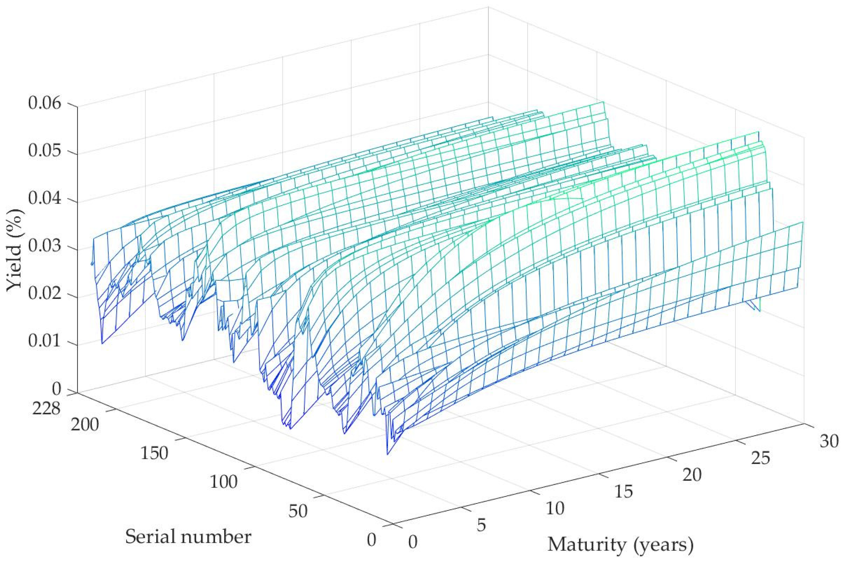
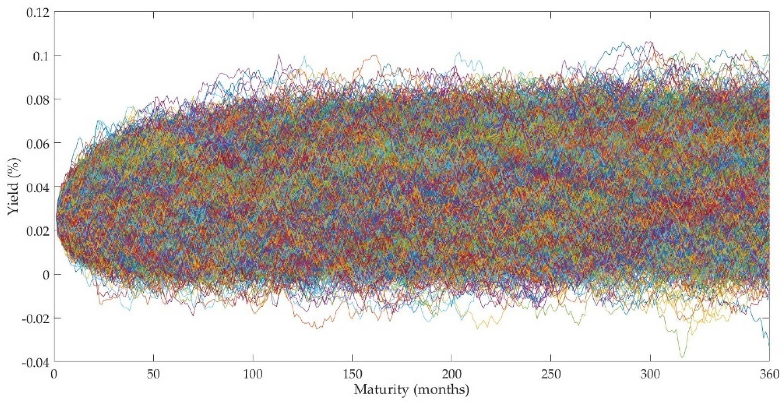
4. Empirical Simulation Analysis

4.1. Basic Conditions and Assumptions of the Project

Based on the toll rights, a commercial expressway project along the southeast coast of China intended to issue redeemable asset-backed notes (ABN). We analyzed the historical traffic flow and growth of many expressways along the southeast coast of China. Furthermore, we found that most of the expressways had a linear increase in tolls within 7–8 years after construction, and then the annual tolls had fluctuated within a stable range. Therefore, this paper used the Monte Carlo method to simulate the cash income of vehicle tolls for a new expressway in the next 30 years. The basic assumptions for the pricing of expressway income rights securities were:
(1) There was no major change in the social, political, and economic environment of the area where the expressway company was located.
(2) The expressway toll rights operated by the expressway company during the forecast period remain unchanged and the toll standards remain stable.
(3) There was no major change in the operating environment, operating conditions, and market conditions of the expressway company during the forecast period.
(4) During the duration of the securities, the subject of the securities issuance could carry out a redemption operation every five years, and the agreed redemption price was CNY 104. When the price of the securities was higher than the execution price, the securities issuer would perform the redemption operation.
Assuming that the tolling period of the project was 30 years and operating costs accounted for 20% of the toll amount, the net cash inflow in the first year after the completion of the expressway was expected to be CNY 25 million. In the first eight years, the net cash inflow would be increased by CNY 5 million annually. After the eighth year, the annual net cash inflow obeys a normal distribution, with an average value of CNY 60 million and a standard deviation of CNY 8 million. The overall credit rating of the underlying assets was AAA, and the pricing time was 1 December 2020. Then, we would determine the issuance scale and coupon rate of ABN based on the assumptions.

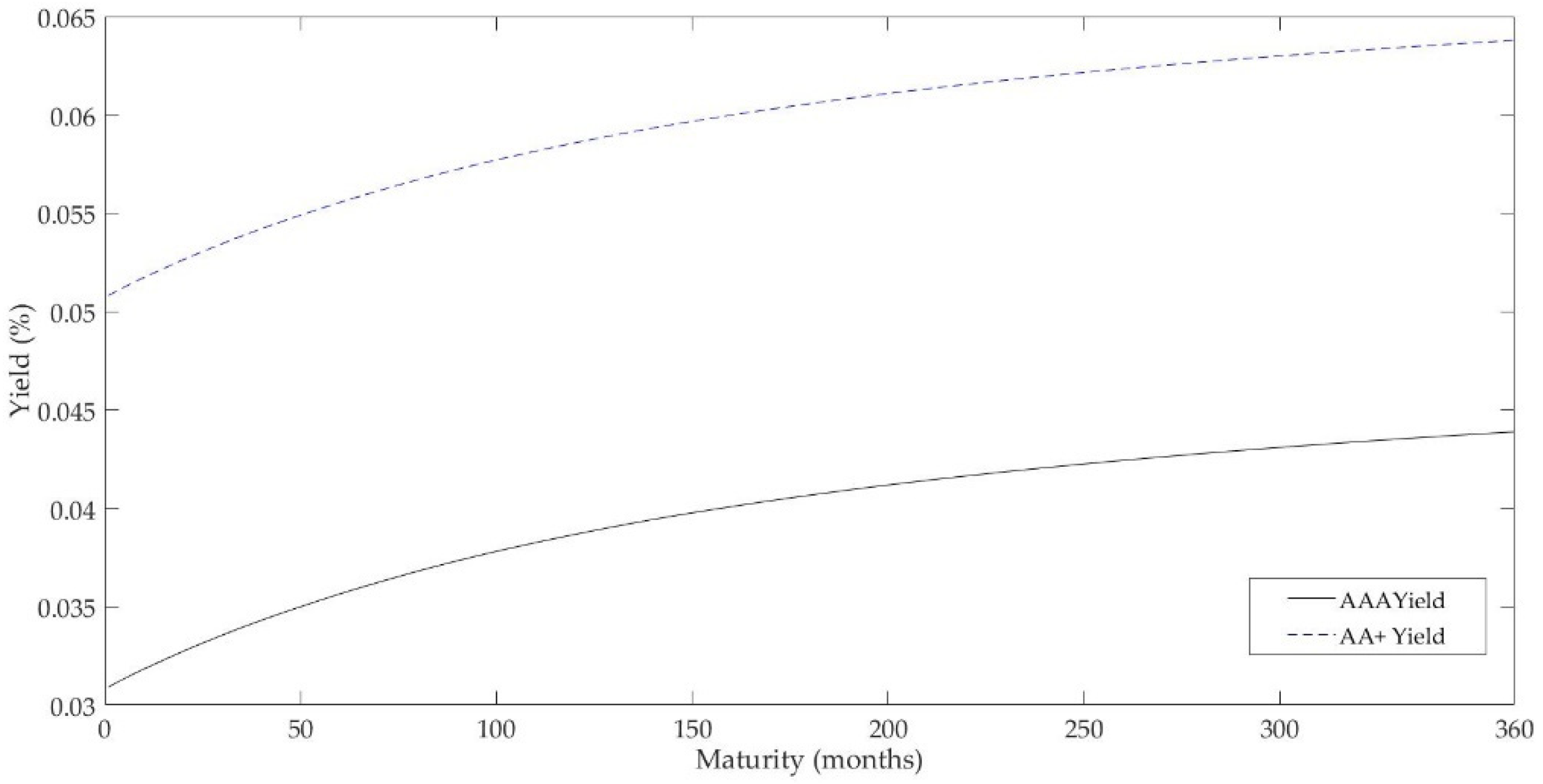
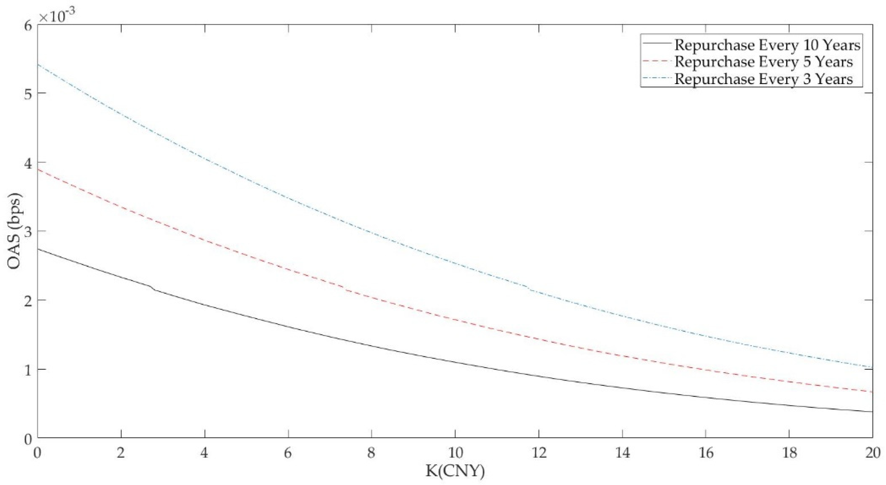
4.2. Redeemable ABN Pricing

The first step was to predict the net cash flow of each period in the future. The net cash flow N C F t of the expressway in each future period was:
N C F t = { 2000 + 500 t , t = 1 , , 8 N ( 6000 , 800 ) , t = 9 , ...30
The second step was to fit the yield to maturity curve. Since the two factors of the two-factor Vasicek model were not observable, the Kalman filter method has been used mainly for parameter estimation. However, this method required observations of spot interest rates as data. Therefore, the static estimation method of the term structure of interest rates should be used to generate spot interest rate data. This paper chose the SV model as the static estimation method.
We used the bond data on 23 January 2009, as an example. Before making an estimate, the data should be filtered. The price of bonds with less liquidity could not reflect the market price of bonds truly. Therefore, the transaction amount has become an important indicator of excluding data, as the transaction amount can reflect the liquidity of the bond. We believed that bond data with a transaction value of less than CNY 200,000 should be eliminated. After excluding the data, we drew a two-dimensional graph with the closing rate of return and the remaining maturity as the vertical and horizontal axes based on the remaining data to check whether abnormal points deviated from the group. If it existed, the abnormal data would be removed. After eliminating the data on 23 January 2009, according to the transaction amount, there was no abnormal data. Therefore, no further removal was required.
After filtering the data, the cash flow of each period of the bond could be calculated by the frequency of annual interest payments and the coupon rate. Through the established parameters β 0 , β 1 , β 2 , β 3 , τ 1 , τ 2 , the theoretical price of the bond could be calculated, and then the error between the theoretical price and the actual price of all bonds could be obtained. The parameter combination that minimized the weighted error value was the best parameter estimation of the model. The bond data was estimated using the SV model, and the results were shown in Table 1:
Once the parameter value was determined, Formula (13) could be used to describe the relationship between the spot interest rate and the remaining maturity, and then the spot interest rate curve could be obtained. The spot interest rate curve is shown in Figure 1.
The points in Figure 1 represented the actual data, and the curve was the fitting result of the model, which depicted the relationship between spot interest rates and maturity. The curve in the figure showed an upward trend, the normal shape. Most of the fitting results would produce an increasing interest rate curve. This article used 1-year, 2-year, 3-year, 5-year, 10-year, 20-year, and 30-year spot interest rate data as the dynamic estimation data. Therefore, Formula (13) had to be used to generate these spot interest rate data. The spot interest rate data on 23 January 2009, was shown in Table 2.
Using the above estimation method, this article calculated the spot interest rate data on the last trading day of each month from December 2001 to November 2020. There was a total of 228 observation days. All bonds’ data were collected from the iFind database. A set of spot interest rate values could be generated every day based on the estimated results of the SV model. Each set of the data contained estimated data on spot interest rates with a period of 1 year, 2 years, 3 years, 5 years, 10 years, 20 years, and 30 years. There were 228 sets of data in total. The 228 sets of spot interest rates for 228 days together constituted panel data. We drew all the spot interest rate data into a three-dimensional graph, as shown in Figure 2.
The data used in the Kalman filter was generated by the SV model. The δ 0 , δ 1 , δ 2 , λ 1 , λ 2 , q 1 , q 2 parameter results required by the two-factor Vasicek model were shown in Table 3.
This research calculated the price B i ( t ) of the national debt on each interest rate path at the redeemable time points: the 5th, 10th, 15th, 20th, and 25th years using the obtained parameters and the two-factor Vasicek model. Figure 3 showed generate 10,000 interest rate paths. When B i ( t ) < K ( K was the agreed execution price), bond redemption occurred. At the moment of redemption, the bond buyer’s income was K . The cash flow after the redemption moment was cleared, and the present value of the cash flow of each interest rate path was calculated to obtain the theoretical price B i of the national debt with rights. The option adjustment spread superimposed on the term structure of the treasury bond interest rate was changed, so to make the theoretical price of the treasury bond equal to the value of the treasury bond with rights, and then, the option adjustment spread o n s was obtained. The yield rate of the 30-year treasury bond obtained by the simulation was 3.97%. When the face value of the bond was CNY 100 and the agreed price K   = 104 CNY, the option adjustment spread o n s   = 30 bps was calculated.
Then, the credit spreads of different grades of corporate bonds were calculated. The closing prices of 14 AAA-rated and 9 AA+-rated corporate bonds without rights on December 1, 2020, as the fitted price data was selected to calculate the Z spread of each bond. It was obtained that the 30-year Z spread of AAA bonds was 15 bps, and the average Z spread of AA + bonds was 214 bps.
The Z spread and the ONS spread on the benchmark interest rate curve of the national debt to obtain the yield-to-maturity curves of bonds with different credit ratings are superimposed, as shown in Figure 4.
After that, this research determined the issuance scale of bonds of different grades. The most stable cash flow part of expressway future income constitutes priority A-level bonds, with a credit rating of AAA, and N C F t A A A was determined by Formula (27):
N C F t A A A = { 1000 + 500 t , t = 1 , , 8 40,000 , t = 11 , , 20
Formula (4) determined that the bond issuance scale of priority A bond was CNY 510 million.
Assuming that assets with a credit rating of AA+ constitute the basic assets of a priority B bond, the cash flow of a B bond N C F t A A + was determined by Formula (28).
N C F t A A + = { 800 , t = 1 , , 8 N ( 800 , 600 ) , t = 9 , , 20 3000 , t = 21 , , 25  
The B-level bond issuance scale was CNY 125 million.
The cash flow of subordinated bonds was:
C F t B = { 200 , t = 1 , , 8 N ( 200 , 200 ) , t = 9 , , 20 N ( 3000 , 800 ) N ( 6000 , 800 ) , , t = 21 , , 25 t = 25 , , 30
This part was not issued and held by the issuer.
Then we obtained the parity coupon rates of A-grade bonds and B-grade bonds, which were 4.29% and 6.58% respectively, and the total issuance scale was CNY 635 million.
After that, the sensitivity analysis on the ABN product pricing model was conducted. Assuming that bonds were issued at a fair price, the coupon rate of the bonds was the implicit rate of return. Formulas (6) and (7) were used to calculate the price changes of different grades of bonds under different yield changes, as shown in Table 4. It can be seen from the table that senior B bonds in ABN had lower interest rate sensitivity than senior A bonds. When the yield fluctuates slightly, the bond price did not change much. It had a greater impact on bond prices only when the yield changed greatly.
Theoretically, the higher the frequency of agreed redemption, the more opportunities the bond issuer could redeem, the more favorable it was for the bond issuer, and the higher the OAS should be. Meanwhile, the higher the execution price K , the higher the compensation to investors, the more benefits to investors, and the lower the OAS should be.
This research simulated the impact of changes in agreed repurchase frequency and execution price on OAS, as shown in Figure 5. Three lines in the figure represented that the agreed repurchase frequency was once every 3 years, the agreed repurchase frequency was once every 5 years, and the agreed repurchase frequency was once every 10 years from top to bottom respectively. For the same K value, the OAS corresponding to the agreed repurchase frequency once every 3 years was greater than the agreed repurchase frequency once every 5 years, and the latter one was greater than the agreed repurchase frequency every 10 years. The simulation results fitted the theory. The higher the agreed repurchase frequency, the higher the corresponding OAS compensation. From a horizontal perspective, as the K value increases, the trends of the three curves are the same, with OAS showing a decreasing trend, which reflects that the simulation results match the theory. The higher the agreed buyback frequency, the higher the corresponding OAS compensation. The empirical simulation results were consistent with theory and common sense, which proved that the method proposed in this research was robust and technically logical.

5. Conclusions

The United States, Japan, and other developed countries have made substantial progress in the field of securitization of infrastructure projects, which indicates China’s securitization of infrastructure projects has a huge potential. However, in the United States or China, there is still a lack of research on securitization products of infrastructure projects. This article proposes the steps for the issuance of redeemable asset-backed notes (ABN) with infrastructure project income rights as the basic asset based on the main body and project characteristics of the infrastructure project securities issuance. The method simulates the stochastic interest rate term structure and interest rate path, which superimpose the cash flow corresponding to each interest rate path accordingly and calculated option-adjusted spread (OAS). This paper put forward a new method to replace the traditional method. Taking the expressway franchise as an example, the article determines the issuance scale and coupon rate of the redeemable ABN based on the expected cash flow of the expressway, the term structure of random interest rates, and the OAS. Furthermore, the duration, convexity, and OAS have been analyzed. It finds that the OAS obtained by the simulation calculation is affected by the agreed repurchase frequency and the repurchase execution price. The OAS is positively correlated with repurchase frequency and negatively correlated with the execution price of agreed repurchase. This conclusion is consistent with theory and common sense, which proves that the method proposed in this study is scientific and practical.
This paper designs the redeemable asset-backed notes (ABN) based on the infrastructure projects’ usufruct as the underlying assets, which solves the pricing problem of redeemable asset-backed securitization products in the field of infrastructure. This study mainly refers to the pricing idea of American options, providing detailed pricing steps for the local governments of China to issue infrastructure securitization products. Further research could be conducted in the following areas: (1) accurate prediction and stratification of cash flow for infrastructure projects; (2) pricing issues of puttable securitization products of infrastructure projects; (3) the transaction structure and pricing issues of REITs with infrastructure income rights; and (4) more practical trading structure of redeemable infrastructure asset-backed securitization products.

Author Contributions

Conceptualization, Q.Z.; methodology, Q.Z.; software, Q.Z.; validation, L.Y.-n.T., B.W. and A.E.; data curation, Q.Z.; writing—original draft preparation, Q.Z.; writing—review and editing, Q.Z., L.Y.-n.T., B.W. and A.E.. All authors have read and agreed to the published version of the manuscript.

Funding

This research was funded by the National Natural Science Foundation of China, grant number 71973009.

Institutional Review Board Statement

Not applicable.

Informed Consent Statement

Not applicable.

Data Availability Statement

The data that support the findings of this study are available on the iFind database and the WIND database.

Conflicts of Interest

The authors declare no conflict of interest.

References

  1. Wang, D.; Li, Z.; Zhao, Z.; Zhao, X.B. Urban Infrastructure Financing in Reform-era China. Urban Stud. 2011, 48, 2975–2998. [Google Scholar] [CrossRef]
  2. Pan, F.; Zhang, F.; Zhu, S.; Wojcik, D. Developing by borrowing? Inter-jurisdictional competition, land finance and local debt accumulation in China. Urban Stud. 2017, 54, 897–916. [Google Scholar] [CrossRef]
  3. Filipović, D.; Willems, S. A term structure model for dividends and interest rates. Math. Financ. 2020, 30, 1461–1496. [Google Scholar] [CrossRef]
  4. Sheraz, M.; Preda, V.; Dedu, S. Non-extensive minimal entropy martingale measures and semi-Markov regime switching interest rate modeling. Aims Math. 2020, 5, 300–310. [Google Scholar] [CrossRef]
  5. Rojo-Suárez, J.; Alonso-Conde, A.B. Relative Entropy and Minimum-Variance Pricing Kernel in Asset Pricing Model Evaluation. Entropy. 2020, 22, 721. [Google Scholar] [CrossRef] [PubMed]
  6. Liao, Z.; Zhang, H.; Guo, K.; Wu, N. A Network Approach to the Study of the Dynamics of Risk Spillover in China’s Bond Market. Entropy. 2021, 23, 920. [Google Scholar] [CrossRef] [PubMed]
  7. Dunsky, R.M.; Ho, T.S. Valuing Fixed Rate Mortgage Loans with Default and Prepayment Options. J. Fixed Income 2007, 16, 7–31. [Google Scholar] [CrossRef]
  8. Jacob, D.P.; Hong, T.C.H.; Lee, L.H. An Options Approach to Commercial Mortgages and CMBS Valuation and Risk Analysis. The Handbook of Non-agency Mortgage-backed Securities; Wiley: Grafton, NH, USA, 2000; pp. 465–495. [Google Scholar]
  9. Sharp, N.J.; Newton, D.P.; Duck, P.W. An Improved Fixed-Rate Mortgage Valuation Methodology with Interacting Prepayment and Default Options. J. Real Estate Financ. Econ. 2008, 36, 307–342. [Google Scholar] [CrossRef]
  10. Liu, Z.Y.; Fan, G.Z.; Lim, K.G. Extreme Events and the Copula Pricing of Commercial Mortgage-Backed Securities. J. Real Estate Financ. Econ. 2009, 38, 327–349. [Google Scholar] [CrossRef]
  11. Hürlimann, W. Valuation of Fixed and Variable Rate Mortgages: Binomial tree versus analytical approximations. Decis. Econ. Financ. 2012, 35, 171–202. [Google Scholar] [CrossRef]
  12. Qian, X.S.; Jiang, L.S.; Xu, C.L.; Wu, S. Explicit formulas for pricing of callable mortgage-backed securities in a case of prepayment rate negatively correlated with interest rates. J. Math. Anal. Appl. 2012, 393, 421–433. [Google Scholar] [CrossRef] [Green Version]
  13. Fan, G.Z.; Sing, T.F.; Ong, S.E. Default Clustering Risks in Commercial Mortgage-Backed Securities. J. Real Estate Financ. Econ. 2012, 45, 110–127. [Google Scholar] [CrossRef]
  14. Fermanian, J.D. A Top-Down Approach for Asset-Backed-Securities: A Consistent Way of Managing Prepayment, Default and Interest Rate Risks. J. Real Estate Financ. Econ. 2013, 46, 480–515. [Google Scholar] [CrossRef]
  15. Hayre, L.S. Understanding Option-adjusted Spreads and Their Use. J. Portf. Manag. 1990, 16, 68–69. [Google Scholar] [CrossRef]
  16. Green, R.K. Chapter 11-The Yield Curve, Monte Carlo Methods, and the Option-Adjusted Spread. In Introduction to Mortgages & Mortgage Backed Securities; Elsevier Inc.: Amsterdam, The Netherlands, 2014. [Google Scholar]
  17. Dong, J.C.; Liu, J.X.; Wang, C.H.; Yuan, H.; Wang, W.J. Pricing Mortgage-Backed Security: An Empirical Analysis. Syst. Eng.-Theory Pract. Online 2009, 29, 46–52. [Google Scholar] [CrossRef]
  18. Vasicek, O. An Equilibrium Characterization of the Term Structure. J. Financ. Econ. 1977, 5, 627. [Google Scholar] [CrossRef]
  19. Vázquez-Vázquez, M.; Alonso-Conde, A.B.; Rojo-Suárez, J. Are the Purchase Prices of Solar Energy Projects under Development Consistent with Cost of Capital Forecasts? Infrastructures 2021, 6, 95. [Google Scholar] [CrossRef]
  20. Falbo, P.; Paris, F.M.; Pelizzari, C. Pricing Inflation Linked Bonds. Quant. Financ. 2010, 10, 279–293. [Google Scholar]
  21. Longstaff, F.A.; Schwartz, E.S. Valuing American Options by Simulation: A Simple Least Squares Approach. Rev. Financ. Stud. 2001, 14, 113–147. [Google Scholar] [CrossRef] [Green Version]
  22. Fabozzi, F.J. Fixed Income Analysis; John Wiley & Sons: Hoboken, NJ, USA, 2007; Volume 6. [Google Scholar]
  23. Nelson, C.; Siegel, A.F. Parsimonious Modeling of Yield Curves. J. Bus. 1987, 60, 473–489. [Google Scholar] [CrossRef]
  24. Svensson, L.E. Estimating and Interpreting Forward Interest Rates: Sweden 1992-1994. Natl. Bur. Econ. Res. 1994. [CrossRef]
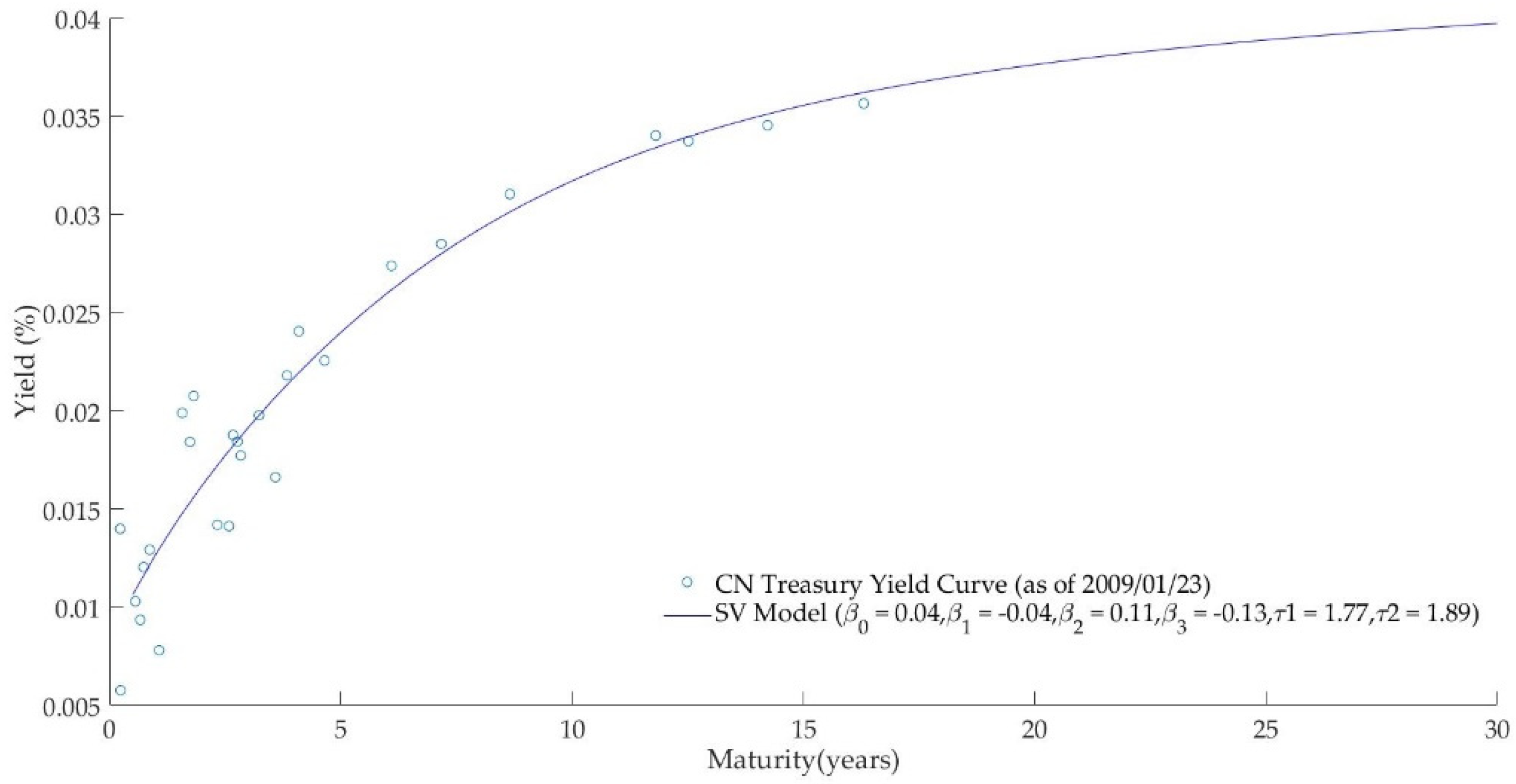
Figure 1. Spot interest rate curve.
Sustainability 13 09113 g001
Figure 2. Three-dimensional diagram of spot interest rates.
Sustainability 13 09113 g002
Figure 3. Ten thousand (10,000) interest rate paths.
Sustainability 13 09113 g003
Figure 4. Maturity yield curves of AAA and AA + bonds.
Sustainability 13 09113 g004
Figure 5. OAS under different repurchase frequency.
Sustainability 13 09113 g005
Table 1. Nelson–Siegel model parameter estimation results.
Parameter β 0 β 1 β 2 β 3 τ 1 τ 2
Value0.0421−0.0418340.113045−0.1292131.7730251.887328
Table 2. Spot interest rate data on 23 January 2009.
Maturity (Years)1235102030
Spot Rate (%)0.0113810.0157990.0194730.0251250.0335140.0364710.038727
Table 3. Parameter estimation results of the two-factor model.
Parameter δ 0 δ 1 δ 2 λ 1 λ 2 q 1 q 2  
Value0.05730.02620.01630.20130.08370.04640.0493
Table 4. Price changes of different grades of bonds under yield changes.
Senior A Bonds, Class AAA, Coupon Rate 4.21%, The Issuance Period Is 20 Years
Yield Change (%)DurationConvexity Change (%)Price Change (%)Initial PriceNew Price
+10013.4450−5.411312.243310087.7567
+5013.6753−2.9661−6.387210093.6128
+1013.8575−0.5393−1.322410098.6775
013.90270.00000.0000100100.0000
−1013.94780.53941.3459100101.3459
−5014.12692.69726.9730100106.9730
−10014.34745.392914.5927100114.5927
Senior B bonds, Class AA+, Coupon Rate 6.38%, The Issuance Period Is 25 Years
Yield Change (%)DurationConvexity Change (%)Price Change (%)Initial PriceNew Price
+10013.1436−10.6206−11.949710088.0503
+5013.5989−5.4212−6.280110093.7199
+1013.9720−1.1017−1.308610098.6914
014.06640.00000.0000100100.0000
−1014.16131.11031.3362100101.3362
−5014.54515.63636.9717100106.9717
−10015.033811.478814.7284100114.7284
Publisher’s Note: MDPI stays neutral with regard to jurisdictional claims in published maps and institutional affiliations.

