Estimation of Travel Demand Models with Limited Information: Floating Car Data for Parameters’ Calibration

Abstract

This paper attempts to integrate data from models, traditional surveys and big data in a situation of limited information. The goal is to increase the capacity of transport planners to analyze, forecast, and plan passenger mobility. (Big) data are a precious source of information and substantial effort is necessary to filter, integrate, and convert big data into travel demand estimates. Moreover, data analytics approaches without demand models are limited because they allow: (a) the analysis of historical and/or real-time transport system configurations, and (b) the forecasting of transport system configurations in ordinary conditions. Without the support of travel demand models, the mere use of (big) data does not allow the forecasting of mobility patterns. The paper attempts to support traditional methods of transport systems engineering with new data sources from ICTs. By combining traditional data and floating car data (FCD), the proposed framework allows the estimation of travel demand models (e.g., trip generation and destination). The proposed method can be applied in a specific case of an area where FCD are available, and other sources of information are not available. The results of an application of the proposed framework in a sub-regional area (Calabria, southern Italy) are presented.

1. Introduction

Transport system models (TSMs) support transport planning in the decision-making process that modifies transport systems (TSs). Quantitative estimations of potential effects produced by decisions are necessary to verify that the forecasted (social, economic, and environmental) sustainability goals are pursued [1].

In recent years, Information and Communication Technologies (ICTs) have produced a large quantity of observed data (big data). Generally, big data enriches information from traditional data, in terms of volume and variety. Common tools collect, manage, and process big data within a tolerable elapsed time to improve the representation of real phenomena and their modelling [2]. In the case of TSMs, big data offer new insights into real phenomena related to transport supply and demand components and their interactions.

Notably, this information and data are limited to historical, or real-time, TS configurations at time t (see Figure 1). If decisions concern future TS configurations at the time t + Δt, TSMs are necessary to forecast potential effects, which requires the implementation of a decision support system (DSS; Figure 1). The observed data (obtained from ICT) are input both for the DSS and for TSMs building, in order to estimate the current conditions of transport system (at time t), and for the transport planning process as they concur, together with forecasted data, to predict potential effects on transport system (at time t + Δt). It is worth noting that transport planning process could be fed only by observed data coming from ICT (as it frequently happens in practice), but it is important to be aware of the severe limitations due to the absence of a DSS and TSMs (e.g., no changes are forecasted in demand elasticity if a new mode alternative is present at t + Δt).

In the same real context, the real time data relative to the transport system may be not available because a monitoring system is not present or because the analyst typically does not have a sufficient budget to acquire data. Also in this context, models for transport planning need to be defined.

A preliminary activity in a DSS building process is collecting data and information on TS components (travel demand, transport supply, supply–demand interactions). Part of these data is obtained from specific surveys that if performed with traditional methods, could be expensive. Data from traditional surveys are essential for the parameters’ calibration of TSMs. The combination of ICTs, for data collection, and TSMs inside a DSS, for simulating future configurations of TS, constitutes an ITS (see [3]).

Data obtained from different ICT tools are a precious source of information on TS. Each data source (e.g. mobile phones, smart cards, GPS) has advantages and limitations in providing information and data on the travel demand of private and public TSs [4,5,6]. In general, traffic data are obtained from several types of sources. In these cases, data elaborations imply specific issues related to data fusion [7]. In other cases, for example the specific context of this paper, a traffic monitoring system is not available, or the data provided are not public; therefore, floating car data (FCD) are the only low-cost source available in a short time to obtain traffic flow data, considering that today, many vehicles have an embedded GPS. However, substantial effort is necessary to filter, integrate, and convert them to be useful for building travel demand models. Moreover, big data refer to historical, or at most, real-time, mobility patterns.

The use of observed data for forecasting TS configurations, without the support of TSMs, can be adopted for ordinary conditions where the TS repeats its configuration cyclically in space and in time (the absence of not-systematic disturbances). In this case, statistical approaches (e.g., Kalman filtering, neural network) provide reliable forecasts. When exogenous non-systematic disturbances occur (e.g., emergency conditions determining demand peaks, for example evacuation, and/or network modifications, for example links’ closure), the TS forecasts are obtained from a combined use of historical data, TSMs, and real-time data.

TS configuration forecasts, obtained from data elaborations and TSMs, could support transport planning at different temporal dimensions and with different levels of approximation. According to the quality and quantity of available data and the model typology, it is possible to predict TS configurations on short-term and/or long-term horizons (e.g., implementation of new transport infrastructures or services). Short-term transport planning, because TSs are dynamic, non-stationary, and uncertain, requires real-time data to run on-line models based on artificial intelligence. These models might influence activity and/or travel users’ choices [8]. Long-term transport planning requires a combination of traditional data and historical data to enhance classical transport models. The results of these models are useful for transport operators and public and private decision-makers to perform ex ante and ex post evaluations of TS configurations in the medium-long term.

Travel demand models support transport analysts and planners in forecasting mobility, generated in planned scenarios of TS. The model building is generally based on a specification–calibration–validation process. Although travel demand models have become more sophisticated, the building process is mainly based on data from traditional surveys (travel diary surveys, census and traffic counts), which are expensive.

In the literature, a research line has investigated the possibility of integrating traditional data and FCD to obtain quantitative estimations of travel demand related to historical and real-time TS configurations. Some authors have proposed methodologies to estimate travel demand behaviour or origin-destination (OD) flow matrices, by means of observed statistics or inferential analysis (a detailed state of the art is reported in Section 2). The main limitation of these studies is the modelling capacity to estimate effects produced by planned TS configurations in technologically advanced contexts, where it is possible to acquire varied and copious information on the TS. Studies that have focused on territorial contexts, which are poorly provided by ICT for transport, are uncommon.

This paper focuses on classical travel demand models based on a network approach and enhanced with FCD elaborations to support transport planning in the medium-long term.

The general objective of the research is to integrate traditional data and data provided by different ICT tools inside an ITS to improve TMSs’ accuracy of estimation, also in a context where there is a scarcity of available data (e.g., no traffic monitoring systems present, traffic data not publicly available).

The specific objective of this paper concerns the increase of the accuracy of travel demand models with FCD, with a focus on a trip’s generation and distribution levels. In particular, commercial FCD should support the analysis of TSs, to obtain demand estimations in future scenarios. The paper is also concerned with the use of commercial FCD in a sub-regional area, characterized by a low level of technologies for transport monitoring, to support strategic transport planning.

This paper’s research contribution concerns the proposition of a framework to estimate travel demand models that starts from initial demand parameters and is updated by means of FCD. This framework allows interactions and synergies among data derived from traditional surveys, FCD derived from GPS, and traditional methods and models for travel demand estimation (trip generation and distribution models). The application of the proposed methodology supports quantitative evaluations of social, economic, environmental and climate issues related to road mobility. The proposed framework reduces the costs of traditional surveys on components of TS, using commercial FCD, albeit with information limited to the space–time positions of road vehicles. The paper also presents an experiment to analyse the current (and future) passenger mobility inside a sub-regional area, near a touristic port (Calabria, in the south of Italy).

After this introduction, the paper presents four sections. Section 2 reports a state of the art of the following two items. The former regards the main ICT technologies providing data used for supporting the estimation of characteristics of users’ trips at the generation and distribution level. The latter concerns the travel behaviour and the OD flow matrices’ estimation through FCD, by means of observed statistics or inferential analysis. Section 3 illustrates the proposed framework for travel demand analyses (generation and distribution models). Section 4 reports the principal results of the framework’s experimentation in the sub-regional area. The last section provides conclusions and research perspectives.

2. State-of-the-Art: FCD Applications for Travel Demand Estimation

This section presents a state of the art concerning the estimation of passenger travel demand models with FCD and it is articulated into two parts. The first part reports a classification of technologies able to obtain data for the estimation of characteristics of users’ trips at the generation and distribution level. The second part reports some methodologies that use FCD to estimate travel behaviour and OD flow matrices.

2.1. Information and Data

Information and data for the estimation of travel demand models are traditionally classified into data on socioeconomic characteristics of users, land use, characteristics of users’ trips and behaviour, and travel costs in a transportation network. Today, several technologies provide big data related to one or more of the aforementioned classes.

In relation to the objective of this research, namely, the estimation of characteristics of users’ trips at the generation and distribution level, four main type of data may be obtained from existing technologies, or social media [4,6]: mobile phones, smart cards, GPSs, and point of interests (POIs).

Mobile phone, or call detail record (CDR), data provide information on large samples of travelers for long periods at negligible costs, when compared with traditional surveys. However, the accuracy of information depends on the distribution of the cells and it is probabilistic because the cells are not closed units but open angles. The frequency of the location updates is conditioned upon a user’s usage. The general challenge of mobile phone data is the extraction of reliable trip sequences and their association to a traveler’s characteristics (e.g., trip purpose [9]).

Smart card data are obtained from automated fare collection (AFC) systems, which are commonly used by public transport operators. While ensuring flexible, secure fare collection, AFC allows for collecting space–time information (on the location of transaction), which is a precious source of trip data on transit users. The main limitation in smart card data is that many AFC systems operate tap-in only (i.e., only boardings are recorded). In general, smart card data support the estimation of OD flow matrices of urban public transport [10].

GPS data, because of the high spatial–temporal resolution, are widely used in mobility applications [11], for example, monitoring vehicles owned by private users and by companies (cars and commercial vehicles for insurance companies) and public transport services (bus fleet), supporting several vehicle drivers’ applications (e.g., route guidance), toll collection, and travel diary surveys. An open question about GPS data concerns the accuracy of some variables estimation (e.g., travel times) in relation to the penetration rate of vehicles equipped with GPS. Klunder et al. [12] showed that a value of 2.0% of penetration rate seems to be acceptable for estimating vehicle speeds (or in-vehicle time). There are two reasons for this finding. First, they calculated that the value of the average absolute percentage error of the average speed on suburban roads with moderate traffic flow (the majority of roads in the study area) tends to decrease, until it becomes negligible, such as when the penetration rate is greater than 1%. Second, they estimated that a FCD penetration rate of 1.7% corresponds to a relatively high availability (10.0%) of links, where a reasonably accurate average speed can be calculated. Ribero et al. [13] conducted a survey on mode choice by using a sample of 72 individuals in Porto Alegre (Brazil), randomly selected from a two-day travel survey. They showed that regarding the estimation of the in-vehicle time parameter, the model’s fit with the GPS data improved 21.0% more than survey-reported data in simple structures of the mode choice models (as MNL models). The differences decrease until 2.0% when model structures incorporating heterogeneity and correlation among individuals are used. According to [14], the average spatial position error of GPS ranges from 2 meters along suburban roads with an open environment to 15 meters along streets with buildings on both sides (urban canyons).

POIs data, also from geocoded social media, could integrate information (e.g. primary locations as origins/destinations of home/work trips) obtained from previous sources, with information on the purpose of trips to/from secondary locations (dining, shopping, types of leisure activities) [15].

Different sources could provide data belonging to the same class, even when the data could have different levels of approximation. This reason is why a technology-based classification of data sources is preferred in this research. For example, mobile phones and GPSs both provide spatial–temporal positions of users, from which information on users’ trip characteristics and travel costs could be obtained. However, GPSs generally provides data at higher spatial–temporal resolution than mobile phones (which depend on phone-cell dimension). Neither mobile phones nor GPSs directly provide information on trip purposes and socioeconomic characteristics of users.

The estimation of users’ trips at the generation and distribution level requires a high-resolution of spatial–temporal positions of users. The research uses data from GPS, namely, FCD.

2.2. Travel Demand Estimation through FCD (Travel Behaviour and OD Flow Matrices)

A solid research line has managed the possibility of integrating traditional data (e.g., travel diary surveys, census and traffic count data) with big data (e.g. vehicles’ spatial–temporal positions), to support travel demand models’ [16]. According to the authors’ review of the literature, some papers have presented methodologies and case studies on the application of big data (e.g. FCD), sometimes in synergy with traditional data, to estimate travel behaviour or OD flow matrices by means of observed statistics or inferential analysis.

2.2.1. Observed Statistics

Wang et al. [17] investigated driving behaviour through FCD collected in the proximity of the University of Michigan (United States). They combined FCD with geocoded street addresses, land use polygons, aerial photographs, census data, and road attributes and reported the methodological challenges of converting an enormous set of geocoded data points into a meaningful database describing passengers’ trips and tours. Wang et al. [17] also presented detailed characteristics of drivers, which are more complex than those that have generally emerged from traditional travel surveys. Lwin et al. [18] used one-week mobile CDR and a GIS road network model to estimate the hourly link population and flow directions, based on mobile-call activities of origin–destination pairs with shortest-path analysis for the city of Yangon (Myanmar). To gain the actual population size from the number of mobile-call users, they introduced a home-based magnification factor by integrating with the national census. The hourly link population and flow direction dataset are intended to optimize bus routes, solve traffic congestion problems, and enhance disaster and emergency preparedness. Toole et al. [19] presented an end-to-end, flexible, modular, and computationally efficient solution that transforms and integrates raw, massive data into estimates of travel demand and infrastructure performance. The system estimates multiple aspects of travel demand by using CDRs from mobile phones in conjunction with open- and crowdsourced geospatial data, census records, and surveys. They used many existing and new algorithms to generate representative matrices, namely, route trips through road networks constructed by using open and crowdsourced data repositories.

Guo et al. [20] proposed an approach that treats vehicle trajectories as a complex network and uses spatially constrained graph-partitioning methods to find spatial structures and general patterns in trajectories. García-Alberto et al. [21] built origin–destination travel matrices from mobile phone records. Several scenarios were generated to characterize transport zones according to their accessibility at different times of day. Their results indicate that the new sources of geo-located data provide more accurate and realistic information than static or partially dynamic analyses.

2.2.2. Inferential Analysis

Djukic et al. [22] applied principal component analysis to transform high dimensional origin–destination flow matrices into a lower dimensional space with no reduction of accuracy. The method adapts online the parameters from traffic counts to obtain real-time estimations of origin–destination flow demand. The objective of the study of Ribeiro et al. [13] was the evaluation of the influence of different sources of travel data (FCD compared with self-reported) in the building of travel demand models. The results showed that FCD collects travel patterns more precisely, reducing the bias by collecting data from short trips not reported in traditional surveys. The models estimated with FCD showed greater significance because of less measurement error. The cost of processing FCD must be considered, and the self-reported data is less precise because of respondents under/overestimation of travel times. The review work of Chen et al. [16] aimed to stimulate the debate between travel behaviour researchers who have long relied on household travel surveys (traditional data) and big data researchers who have recently used passively generated data (big data). In order to achieve this objective, they introduced key concepts and developments in each field and raised cross-disciplinary ideas in three subareas: (a) behavioural factors, (b) model development, and (c) trip patterns. Wismans et al. [23] used mobile phone (CDR) data to update the TS model of the region of Rotterdam. The CDR raw data were processed into basic information, which was subsequently translated into OD flow information, based on several decision rules. This OD flow information was compared with a traditional estimated a priori OD flow matrix through an annual national household travel survey.

Brederode et al. [7] proposed a ‘common operational picture’ to support strategic transport demand modelling, where different data sources (data from traditional surveys and from ICT) were fused and homogenized. The goal was the elimination of the temporal and spatial inconsistencies between data sources, to obtain better estimations of the level of demands (OD flow matrices) and parameters’ calibrations. Liu et al. [24] proposed a three-step procedure to better anticipate future demand patterns, to allow ride-sourcing companies to define their fleet management strategies. The steps are based on the temporal and spatial clustering approach to estimate hourly and daily origin–destination matrices. Krishnakumari et al. [25] presented an original method for origin–destination flow matrix estimation driven by available speed and flow data. They used principal component analysis to derive additional constraints from the data. The goal was to reduce the under-determinedness of the origin–destination matrix estimation problem.

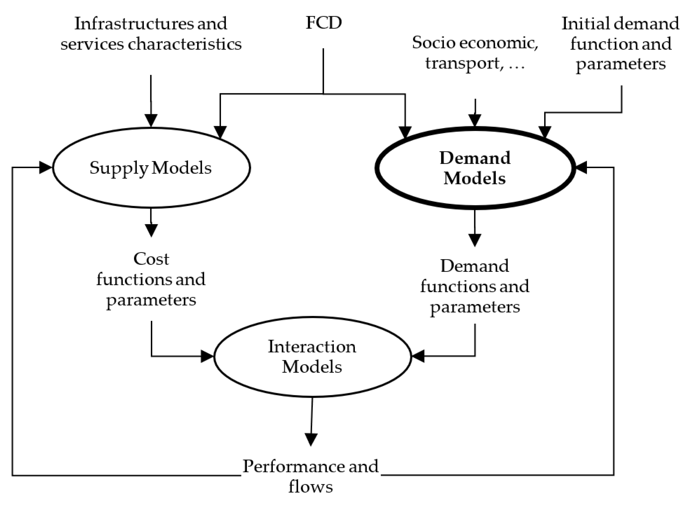
3. Demand Analyses and Models: Generation and Distribution

Traditional and big data enable analyses of TS and its components (supply, demand, supply–demand interactions). TS analyses (Figure 2), with reference to current or future configurations, can be supported by TSMs. They are composed by the following:

• supply models simulating transport infrastructure and services performances in terms of cost functions and parameters;
• demand models simulating people and mobility needs by means of demand functions and parameters; and
• supply–demand interaction models simulating how transport infrastructure and services respond to mobility needs and then TS performances (flows and travel costs).

This paper focuses on travel demand models, especially the people mobility segment.

Travel demand models estimate passengers [26,27,28] and freight trips [29,30] in space and time in relation to specific purposes, transport modes, and paths. Travel demand analysis has been performed by using the approaches in the literature. The classical four-step approach is usually adopted to represent the following travel components: trip generation, trip distribution, mode choice, and route choice. In this paper, the focus is the generation and distribution components.

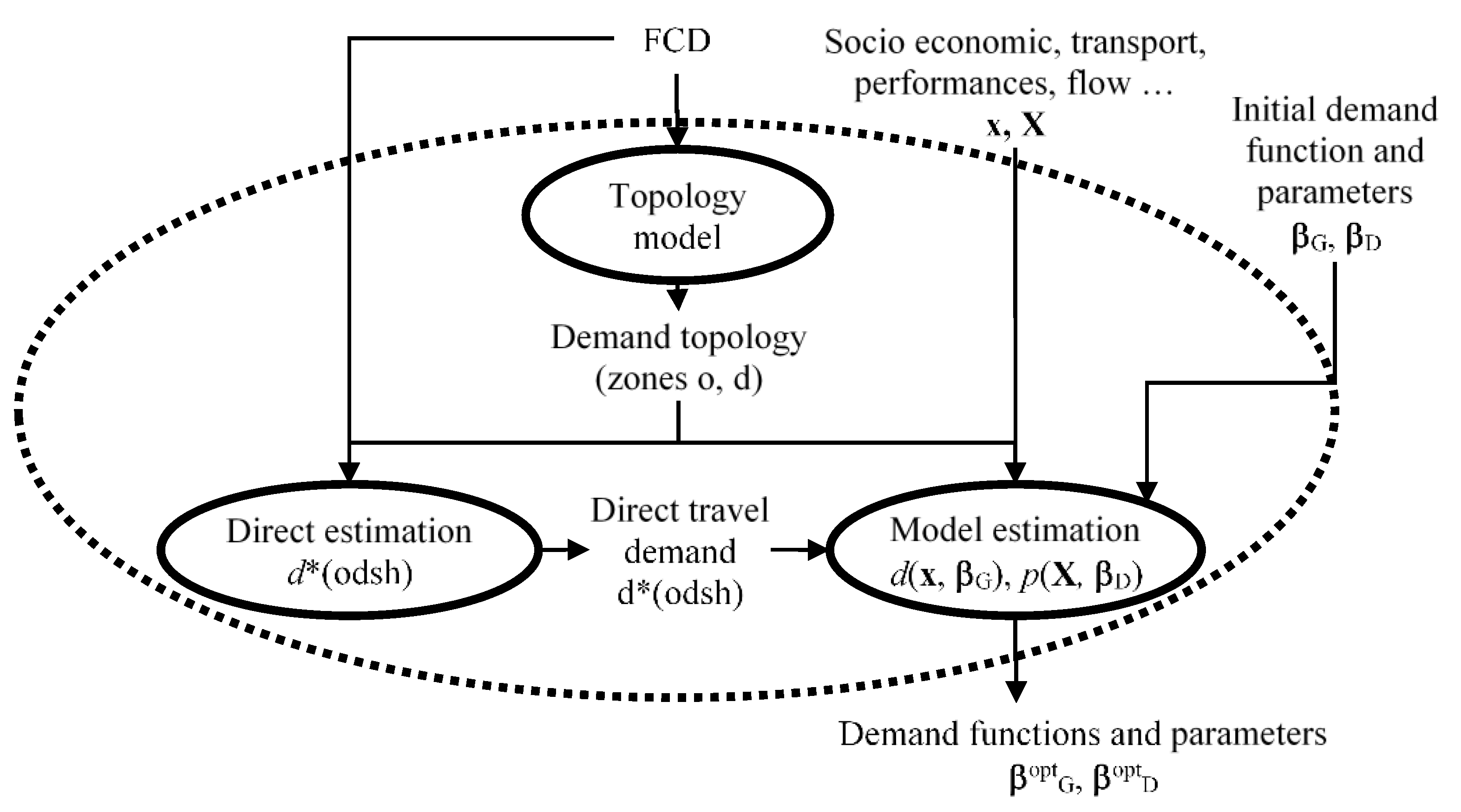
The framework, for the travel demand parameters estimation from only FCD, is reported in Figure 3, where the ellipse of Figure 2 related to ‘Demand Models’ is now enlarged and represented with a dotted line. Figure 3 depicts the data flows, methods, and models to estimate travel demand. The variables adopted, input, and output are reported in this subsection. The model adopted is specified in Section 3.1, Section 3.2, and Section 3.3.

To improve travel demand estimations, FCD can be used. Nevertheless, available data cannot be directly elaborated. A set of operations is necessary, as defined in Section 3.1, to make FCD consistent with the required inputs of travel demand models [31], for what concerns the definition of the study area and the homogenous traffic zones. In particular, traditional data (e.g., socioeconomic characteristics), methods, and models can be enriched with FCD. The topology model, described in Section 3.1, may be combined with traditional zoning techniques to obtain richer, more comprehensive, and more representative information on people’s mobility (e.g., observed trips). The traditional zoning techniques consist in defining homogeneous traffic zones starting from land use and orographic data of the study area. These techniques generate homogeneous zones according to statistical indicators and to planner’s experience. The use of FCD could contribute to the redefinition of this technique, by the introduction of the criterion based on the mobility patterns.

The outputs of the topology model feed the following estimation processes:

• The travel demand direct estimations are obtained by performing statistics of observed trips in relation to historical or real-time TS’s configurations (Section 3.2), providing statistics on historical and/or real-time data.
• The travel demand models estimations are obtained by performing inferential analyses through the elaboration of travel demand direct estimations, starting from the initial demand function and parameters and the socioeconomic, transport, performances, and flow in the initial data. These models simulate a travel user’s behaviour and allow estimations of a decision’s effects related to future TS’s configurations (Section 3.3). The models are built by means of the specification–calibration–validation process from historical and/or real-time data.

Historical data include all the available data referred to similar TS’s configurations. The demand variables are estimated by using the previous estimated values and the observed real time data (e.g., statistic process, time series, …). The time horizon depends on the variables to be estimated (i.e., for the daily demand, the time horizon is the day). The outputs of the model estimation are the demand parameters and the demand specification.

The whole model is reported in Figure 3. The input (or independent) variables are reported with the arrows entering the ellipses (with a solid line) of each individual component. The output (or dependent) variables are reported with the arrows exiting the ellipses. This type of representation is also used in the inner models (topology, direct, estimated).

The input (or independent) variables of the whole model are as follows:

• FCD;
• the vector x and the matrix X containing socioeconomics, land use, transport attributes, network performances at the origin–destination level and flows at the link level; the initial demand function and parameters.

The output (or dependent) variables relative to the estimated demand model are as follows:

• the estimator β^opt_G at the generation level and β^opt_D at the distribution level of the demand parameters.

The whole model can be divided into three sub-models: a topology model, direct estimation, and model estimation.

• Topology Model

The information relative to the topology models is reported in Section 3.1. A statistical method is adopted. The input (or independent) variables of the topology model are FCD that is relative to the observed demand and flow (in general terms, other input variables derived from big data could be used). The socio economic data could be input variables. The output (or dependent) variables of the zoning model are the zoning of the area in terms of homogenous traffic zones, places of origin of the travel o, and destination of the travel d.

• Direct Estimation

The information relative to direct estimation is reported in Section 3.2. A statistical direct estimation method is adopted.

The input (or independent) variables relative to the direct estimation are as follows:

• the zoning of the area in terms of the origins o and destinations d (output of the topology model);
• FCD relative to the observed demand and flow; and
• the number of observed trips from origin zone o to destination zone d, for purpose s and temporal interval h, obtained from sample α, the sampling rate.

The output (or dependent) variables relative to the direct estimation are the estimator of trips d*(odsh) from origin zone o to destination zone d, given the purposes s and the temporal period of trip h. Starting from this output, the emissions, the attraction in each zone, and the aggregation respect the purpose and/or the temporal period and can be obtained.

• Model Estimation

The information relative to the models’ estimation is reported in Section 3.3. A generalised weighted least squares method is adopted.

The input (or independent) variables relative to the estimated demand model are as follows:

• the traffic zones of the area in term of the origins o and destination d (output of the topology model);
• the vector x and matrix X of socioeconomics, land use, and transport attributes, and network performances, at the origin–destination level and flows at the link level;
• the estimator of trips d*(odsh) was obtained as the output of the direct estimation; and
• the initial demand function and parameters β_G at the generation level and β_D at the distribution level.

The output (or dependent) variables relative to the estimated demand model are the same as those in the whole model.

3.1. Topology Model

Traditional zoning methods start from a set of zones identified with the knowledge of land use and quantitative and qualitative criteria. Generally, zoning is an input of transport modelling.

In this paper, a topology model is adopted to generate zoning. The model is fed by big data on transport (e.g., FCD) and land use (e.g., census data). The outputs are the study area and traffic zones.

Big data processing is performed as proposed in [31]. The analyses start from the observations of the available dataset that constitute an input of specific elaborations. The first set of elaborations comprises a spatial analysis of the registered spatial–temporal positions (detected positions). This set of elaborations allows the identification of spatial points of the analyzed area that present a high concentration, and then, it could be trip emission/attraction poles. The study area delimitation represents an output of these elaborations. A second set of elaborations identifies road users’ trips that originated from the detected positions. A generic road user’s trip is characterized by an origin, a destination, and a trajectory, representing a user’s movements without interruptions. While assuming specific filtering criteria, the trajectories are processed to identify road users’ trips. For instance, filters for the application of temporal criteria (e.g. selection of detected positions registered during workdays) and spatial criteria (e.g. selection of trajectories interacting with the study area). The combination of the traditional zoning methods produces as output the demand topology (traffic zones), comprising the discretization of the study area and then the identification of the following:

• the set of the trips’ origins, o; and
• the set of the trips’ destinations, d.

By combining topology and socioeconomic characteristics, it is possible to define a classification of zones. Different sources of data allow the identification of the following:

• the trip’s purpose, s;
• the temporal period, t; and
• the transport mode, m.

Regarding FCD, they contain limited information on trip characteristics. In particular:

• FCD provide no information on trip purposes (s);
• FCD allow the analysis of trips in relation to different temporal periods (h; e.g., 24 h per day); and
• FCD provide information on road vehicles for passengers and freight (the available transport mode m is the road).

3.2. Direct Estimations (Observed Statistics)

Direct estimations consist of elaborating big data to estimate observed travel demand. Information and data on mobility obtained from ICT cannot be directly used. The data necessary data processing concerns the definition and application of a set of filters according to temporal criteria (e.g., selecting positions of vehicles travelling on workdays) and to spatial criteria (e.g., eliminating vehicles’ trajectories outside the study area).

Regarding FCD, single spatial–temporal positions of each vehicle’s travel inside a specific study area are collected. Single positions are grouped into trajectories, representing a vehicle’s trips detected between two consecutive switching-off operations of the vehicle engine. Notably, the trajectories again do not represent real trips from an origin to a destination. Thus, further data aggregation is necessary to convert vehicles’ trajectories into trips. In particular, two consecutive trajectories, separated by a time interval between two vehicle engine actions (e.g., switching on/switching off), defined as temporal lag, might be part of the same trip. The introduction of criteria allows the aggregation of the aforementioned consecutive trajectories into trips. The criteria of aggregation influence the quality of available information on the trips.

Starting with data, travel demand can be estimated by using a simple or stratified random sampling, for example, a sampling travel demand estimator [26]. In relation to the type and quantity of data, it is possible to obtain travel demand estimations for each travel component. These estimations are relative to the historical and/or real-time TS’s configuration.

3.2.1. Generation

According to the demand topology model, the generation component allows the quantifying of each temporal period h and purpose s, the observed trips for each zone o, and n_osh of the study area.

The estimator of generated trips from zone o, for the purpose s and the temporal interval h, can be estimated as follows:

d*(osh) = (1/α) * n_osh    ∀ o, s, h

(1)

where n_osh is the number of observed trips from zone o, for the purpose s and the temporal interval h, obtained from the sample; α is the sampling rate.

The observed demand at generation level can be aggregated for all the purposes s, and it is indicated with d*(oh).

3.2.2. Distribution

According to the demand topology model, the distribution component allows the quantifying of each temporal period h and purpose s, the number of observed trips from origin zone o to destination zone d, n_odsh.

The estimator of trips from origin zone o to destination zone d, given the purposes and temporal period of the trip, is as follows:

d*(odsh) = (1/α) * n_odsh      ∀ o, d, s, h

(2)

where n_odsh is the number of observed trips from origin zone o to destination zone d, for purpose s and temporal interval h, obtained from the sample; α is the sampling rate.

The observed demand at the distribution level can be aggregated for all the purpose s, and it is indicated with d*(odh).

The number of trips towards the destination zone d, in relation to purpose and temporal period, is obtained as the sum extended to all n zones by which the study area is divided:

d*(dsh) = Σ_{o=1, …,n} d*(odsh)     ∀ d, s, h

(3)

3.3. Model Estimations (Inferential Analyses)

Inferential analyses are necessary to quantify the effects of TS’s future configurations. Collected big data, containing information on user’s movements in space and time, can be used for travel demand model estimation. The aim is to infer the physical movements to reproduce user’s behaviour, improving the quality of the estimation.

3.3.1. Specification

(1)

Trip generation

Trip generation models estimate the number of trips from an origin zone o, for the purpose s and the temporal interval h. The number of trips generated from each zone is obtained as follows:

d(osh) = d(x, β_G)     ∀ o, s, h

(4)

where x is the vector of attributes (socioeconomic, transport, …); β_G is the vector of generation parameters.

The demand model at the generation level can be aggregated for all the purposes s, and it is indicated with d(odh).

(2)

Trip distribution

Trip distribution models estimate the percentage/probability of trips undertaken by transport users from the origin zone o to the destination d, given the purpose and the temporal period (sh):

p(d|osh) = p(X,β_D)      ∀ o, d, s, h

(5)

where X is the matrix of attributes (socioeconomic, transport, …); β_D is the vector of distribution parameters.

In relation to each category, purpose, and temporal period considered, the number of trips from the origin o to the destination d is obtained as follows:

d(odsh) = d(osh) * p(d|osh)     ∀ o, d, s, h

(6)

The demand model at distribution level can be aggregated for all the purposes s, and it is indicated with d(odh).

The number of trips towards the destination zone d, given the purpose and the temporal period, is obtained as sum extended to all n zones of the study area:

d(dsh) = ∑_{o=1, …,n} d(odsh)     ∀ d, s, h

(7)

3.3.2. Calibration and Validation of the Generation and Distribution Models

The trip generation and distribution models’ parameters are calibrated by implementing a calibration–validation process, to elaborate traditional and big data from surveys and big data sources.

The calibrated parameters (β^opt_G, β^opt_D) are obtained, minimizing the objective function φ():

β^opt_G, β^opt_D = minimum φ(β_G, β_D)

(8)

where the objective function depends on the initial parameters (β_G, β_D), socioeconomics, transport, performances, flow (x, X), specification of the demand functions (d, p), direct travel demand d*, and a vector of weight (w):

φ(β_G, β_D) = φ(w_i, d*(osh), d*(odsh), d(x,β_G), p(X,β_D))

(9)

The validation comprises a what-if process to search for the minimum value of φ(). The results of the validation process, concerning an increasing level of the goodness-of-fit of the models, can be measured by means of statistical indicators. One indicator considered is the mean square error (MSE):

MSE = ∑_od (d(odsh) – d*(odsh))² / n_od

(10)

where n_od is the number of od pairs. In this paper, the model calibration is performed by applying a generalised weighted least squares method, simultaneously combining the trip generation and trip distribution components. The objective function is expressed as the sum of the squared residuals extended to all n zones:

φ(β_G, β_D) = w_I * ∑_o (d(osh) – d*(osh))²
+ w_II * ∑_od (d(odsh) – d*(odsh))² + w_III * ∑_d (d(dsh) – d*(dsh))²

(11)

where w_I, w_II, and w_III are the weights for the components of the objective function. Notably, one (or more) weight(s) could be assumed to be equal to zero. For instance, by assuming w_II = 0 and w_III = 0, the generation component is considered and the generation model is calibrated.

4. Experiments

The general objective of the experiment is the estimation of the generation and distribution of passengers’ trip patterns in a sub-regional area (Calabria, in south Italy). The focus is on the systematic (e.g., home-work trips) and non-systematic component of the mobility of residents (e.g., home-purchase trips) and non-residents (e.g. local touristic attractions for port users) (see [31,32,33]). A line of the research concerns the estimation of energy consumption of electric vehicles [34].

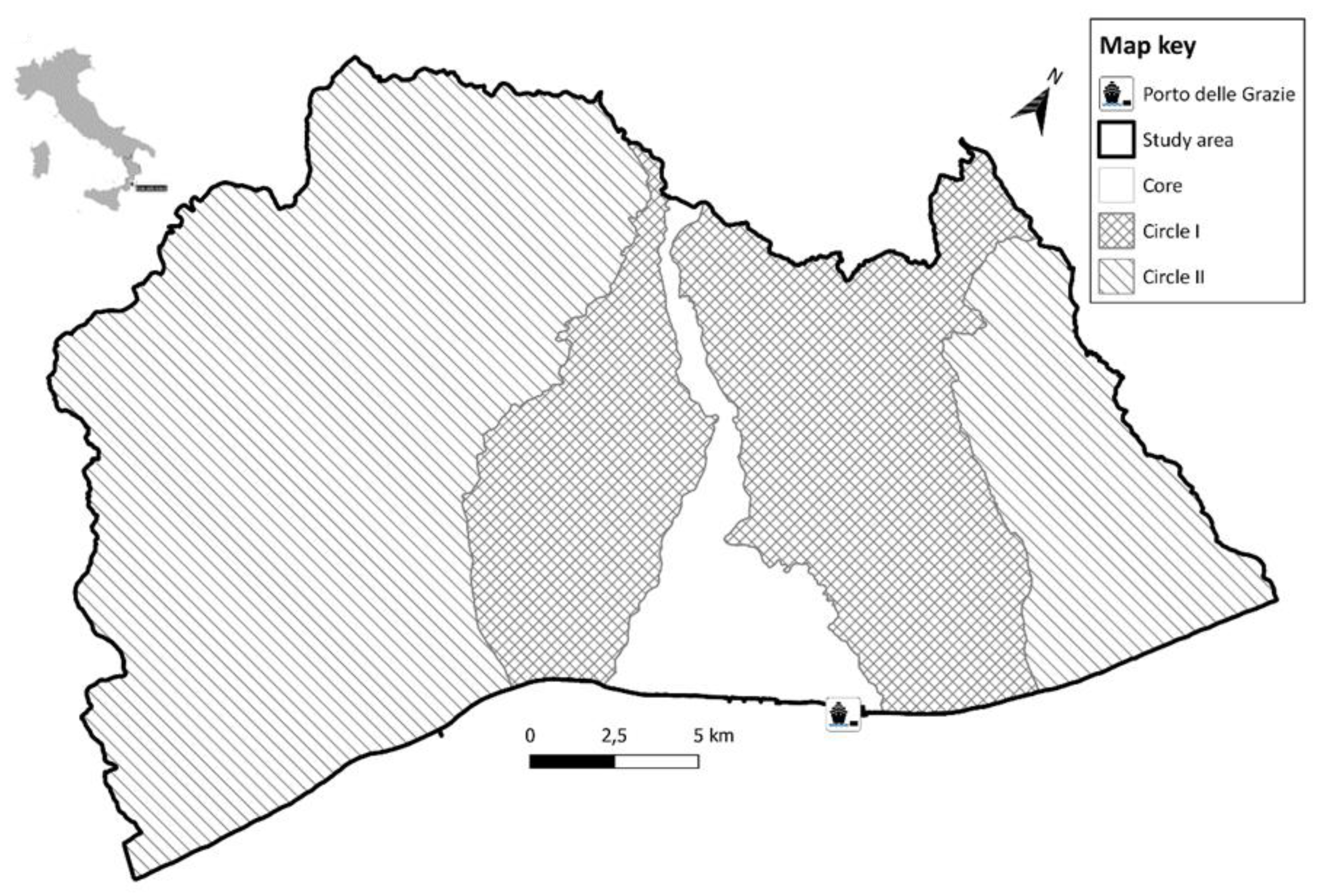
The experiment test site is the backward sub-regional area near an Italian port, ‘Porto delle Grazie’, in the municipality of Roccella Jonica (Città Metropolitana di Reggio Calabria, Italy). Based on the author’s knowledge, the FCD are the available traffic data that is continuous in time and relative to the area.

4.1. Topology Model

The topology model (Section 3.1) has been applied by combining the traditional analysis of socioeconomic census data and FCD as inputs [32,34]. FCD include information on spatial-temporal positions of road vehicles recorded in a period of two winter weeks in 2018.

The topology model provides two main outputs. The intermediate output concerns the identification of the study area (Figure 4), which includes a sub-regional portion close to the port, within the municipality of Roccella Jonica, and sixteen neighboring municipalities. The total population is approximately 72,000 inhabitants, and the number of employees is 14,200. The study area is disaggregated into three parts:

• core, the municipality of Roccella Jonica;
• circle I, the first set of municipalities around Roccella Jonica; and
• circle II, the second set of municipalities.

Output concerns the zoning of the study area into 23 zones:

o ∈ {1; …; 23}

d ∈ {1; …; 23}

The experimentation focused on the following trip purposes:

• C-L    Home-Work
• C-Sc    Home-School
• C-AM   Home-Other

Therefore, the set of purposes is defined as follows:

s ∈ {C-L; C-Sc; C-AM}

The reference period of analysis, h, is a 24-h working day (according to the mobility patterns in the study area, it is considered a working day from Monday to Friday as reference):

h = (00:00; 24:00]

The number of users who use public transport is negligible in the study area. The transit modes are not present as alternatives for urban mobility. Transit modes are used to perform extra-urban journeys. Mobility with the bike is negligible, due to the hilly nature of the study area; bike mode could be an alternative for trips along the coast. Therefore, it is acceptable that the private car mode is the only available motorized mode for trips inside the study area. Motorcycles are not included within the set of available FCD.

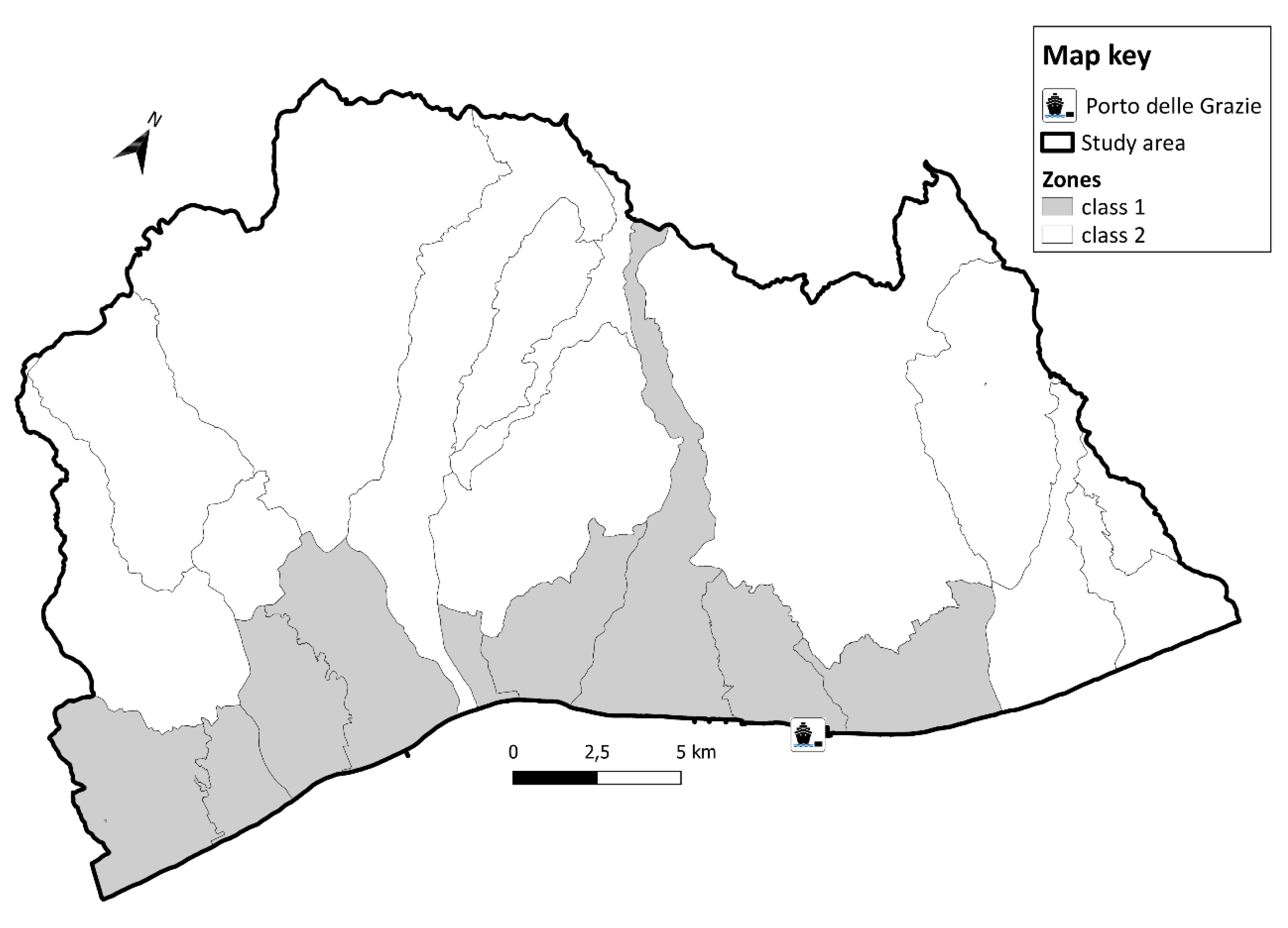
Zones are classified into two classes according to their geographical location inside the study area and the level of the population (Figure 5):

• Class 1, zones less than 1.5 km from the coastline and in municipalities with a population greater than 6000 inhabitants; and
• Class 2, zones far from the coastline, namely, more than 1.5 km away, and zones less than 1.5 km from the coastline in municipalities with a population fewer than 6000 inhabitants.

4.2. Direct Estimation (Observed Statistics)

The available FCD dataset has been used to obtain direct estimations of passenger travel demand in private cars. The number of monitored vehicles is approximately 2% (penetration rate) of the vehicles travelling inside the province of Reggio Calabria.

The penetration rate of vehicles equipped with GPS (2.0%) was assumed as the sampling rate, introduced in Section 3.2.1. According to the existing literature (reported in Section 2.1), the accuracy of the spatial position the of origin/destination of trips is acceptable compared with that of the average dimension of traffic zones and considering that the majority of roads in the study area era extra-urban. Lastly, the authors consider acceptable to assume that the sample is randomly extracted from the fleet of circulating vehicles because FCD are from every segment (private and company cars, commercial vehicles) of the fleet of circulating vehicles. This occurs because a GPS is installed on-board after entering into mandatory insurance contracts with insurance companies.

The number of observed trips and the sampling rate allow the direct estimate of daily trips generated from each zone, d*(oh).

The database contains the following data related to the province of Reggio Calabria during two winter weeks (14 days):

• 2,073,982 spatial-temporal vehicle positions;
• 4498 vehicles for passenger mobility; and
• 361,752 trajectories.

The trajectories are obtained from FCD, and they are defined by connecting consecutive spatial points of vehicles. For this reason, spatial analysis is obtained from the database, and a spatial threshold definition is unnecessary. Therefore, it was possible to build the trajectory of each vehicle as a temporal sequence of positions.

According to the objective of this study, data were selected by considering the spatial–temporal positions and trajectories that referred to 10 workdays of the two winter weeks.

Therefore, the database contains the following data related to the province of Reggio Calabria on 10 workdays (Monday to Friday) during the two winter weeks:

• 4377 different vehicles for passenger mobility;
• 271,109 trajectories.

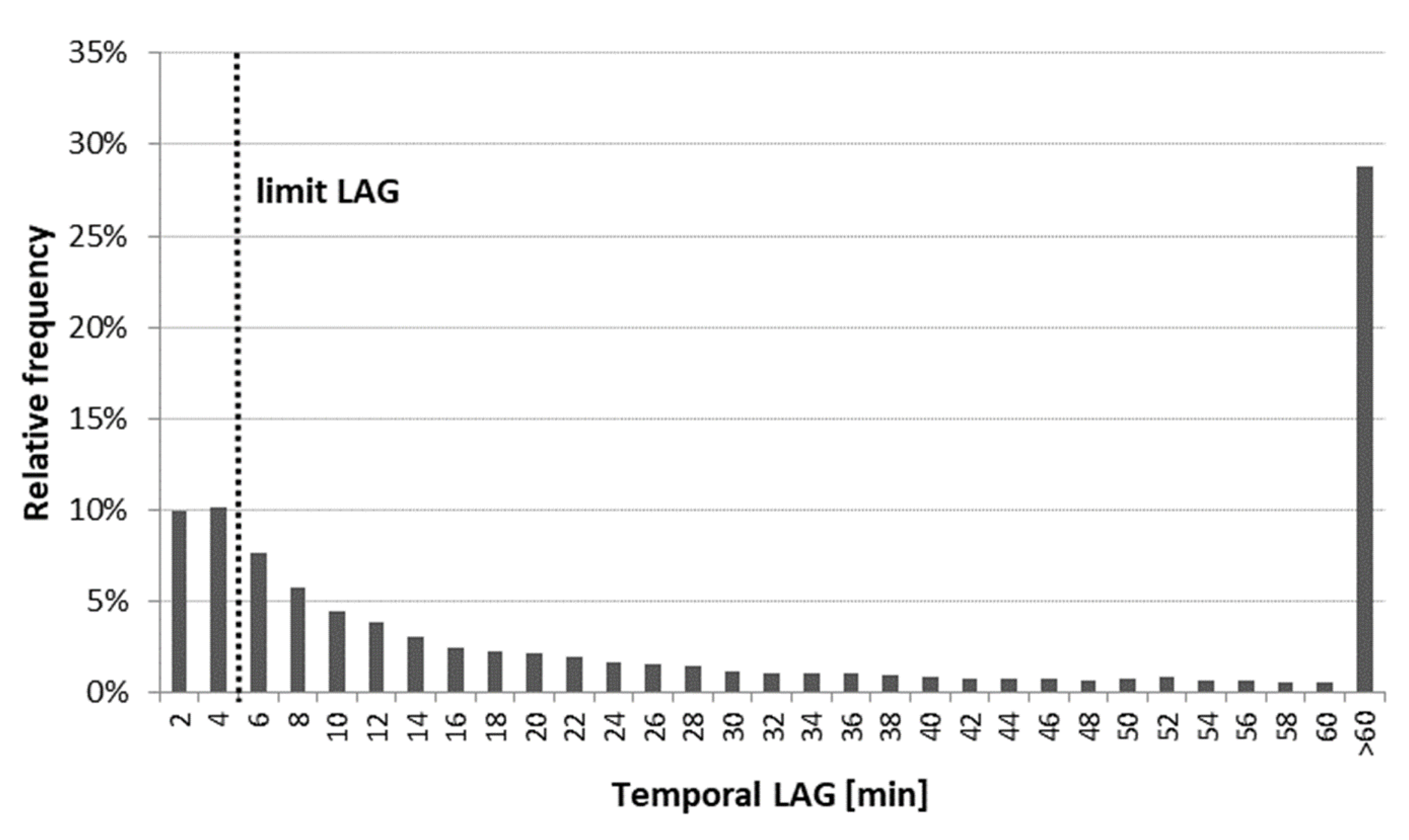
By representing the relative and cumulative frequency of the temporal lags in the available trajectories (Figure 6), the threshold value of temporal lag was identified as the value corresponding to the first reduction of the relative frequency of the lag. Figure 6 shows the threshold value, which is 5 minutes.

The threshold value of temporal lag allows the identification of and the clustering of the trajectories into trips. Therefore, by also considering the lag, the database contains the following data during the 10 workdays (Monday to Friday) during the two winter weeks:

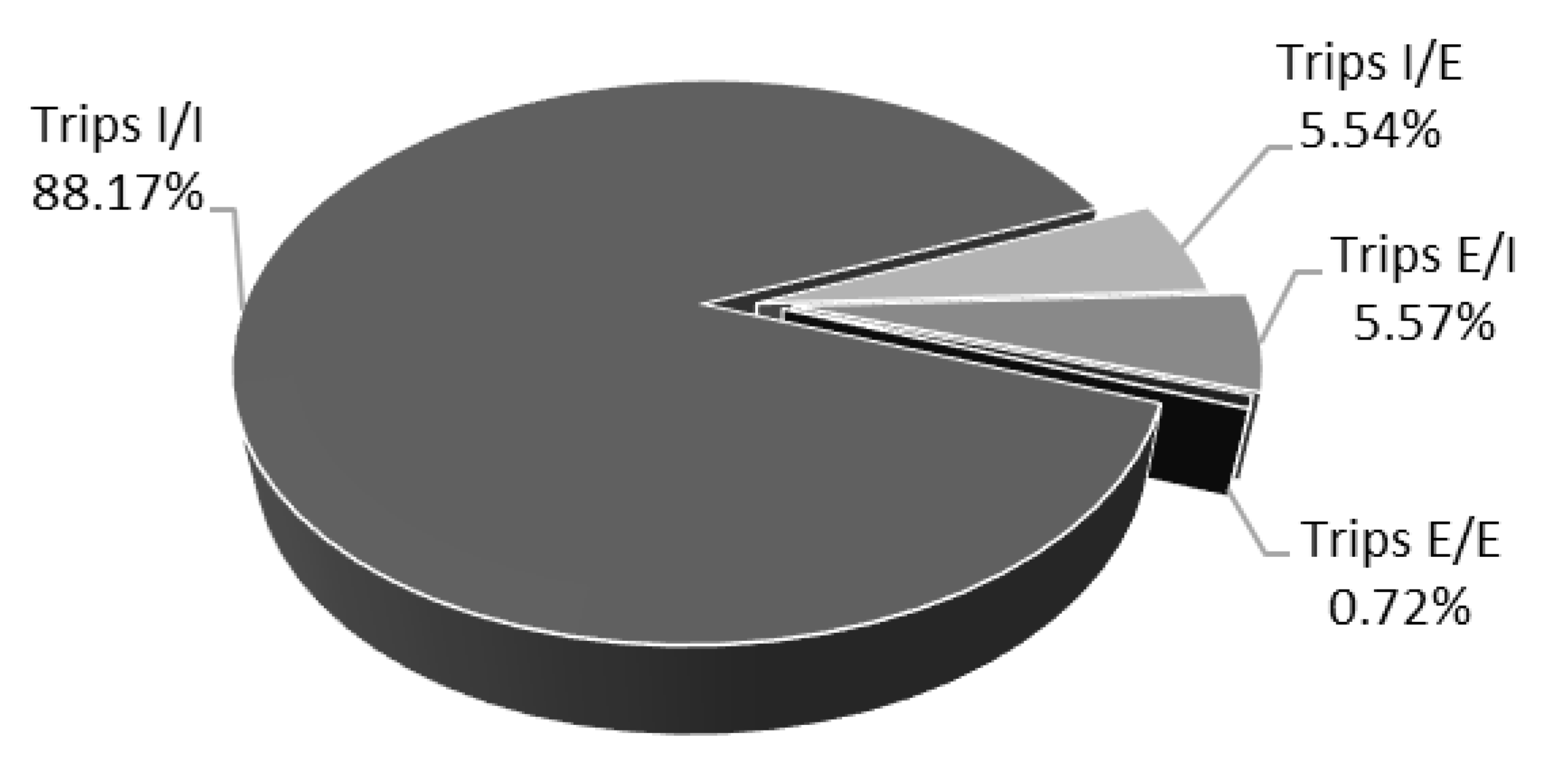
• 213,531 trajectories in the province of Reggio Calabria;
• 24,694 trajectories with at least one spatial–temporal position within the study area; this number comprises trips of four categories: I-I, I-E, E-I, and E-E, according to the origin and destination, which are Internal (I) or External (E) to the study area (Figure 7 depicts the trips’ percentage for each of the four categories);
• 21,774 trajectories with origin and destination within (I-I) the study area; and
• 10,292 trajectories with origin and destination within (I-I) the study area and with inter-zonal trips.

4.2.1. Generation

The data relating to trips in the inter-zonal (I-I) category have been further elaborated to obtain information on their systematic nature. For this purpose, the frequency of trip hour was analysed on an average weekday, starting from the values observed in the reference interval (10 workdays).

Figure 8 shows the distribution of the average number of trips inside each hour with an origin inside the study area. The distribution refers to the observed sample. The figure also shows the values of the standard deviation calculated for each hour.

The low values of the standard deviation show a reduced variability of the hour trips that suggest a systematic nature, more evident at night. The standard deviation reaches higher values in the morning hours and thus demonstrates a greater tendency towards a not-systematic nature of the trips.

The FCD sample of 10,292 trips is used to estimate the number of generated trips, belonging to the inter-zonal I/I category, d*(oh), without indication of the trip’s purpose. The value is divided by the 10 workdays and reported to the “universe” by dividing by the penetration rate (0.02): 51,460 average inter-zonal I-I trips/day are obtained.

The first column in

Table 1. Estimation of the daily distribution matrix (average trips/day).

Origin/Destination		Destination
		All (Generation)	Core	Circle I	Circle II
Origin	Core	4045 (7.9%)	1995 (3.9%)	1310 (2.5%)	740 (1.4%)
	Circle I	13,230 (25.7%)	1320 (2.6%)	6745 (13.1%)	5165 (10.0%)
	Circle II	34,185 (66.4%)	685 (1.3%)	5175 (10.1%)	28,325 (55.0%)
All (attraction)		51,460 (100%)	4000 (7.8%)	13,231 (25.7%)	34,232 (66.5%)

shows the values of the generated inter-zonal I-I trips on an average workday aggregated by considering the three parts of the study area: core, circle I, and circle II.

4.2.2. Distribution

The observed trips and the sampling rate are used to apply the method described in Section 3.2.2., for estimating the number of daily trips from zone o to zone d, relative to all purposes, d*(odh). Notably, as for the generation, the values of the distribution matrix represent the trips for all the purposes considered.

Table 1 shows the values of average daily trips aggregated by considering the three parts of the study area. The values of the trips attracted by each zone are estimated by means of (7). The last row of Table 1 shows the average number of daily trips attracted by each of the three parts of the study area, d*(dh), for all purposes.

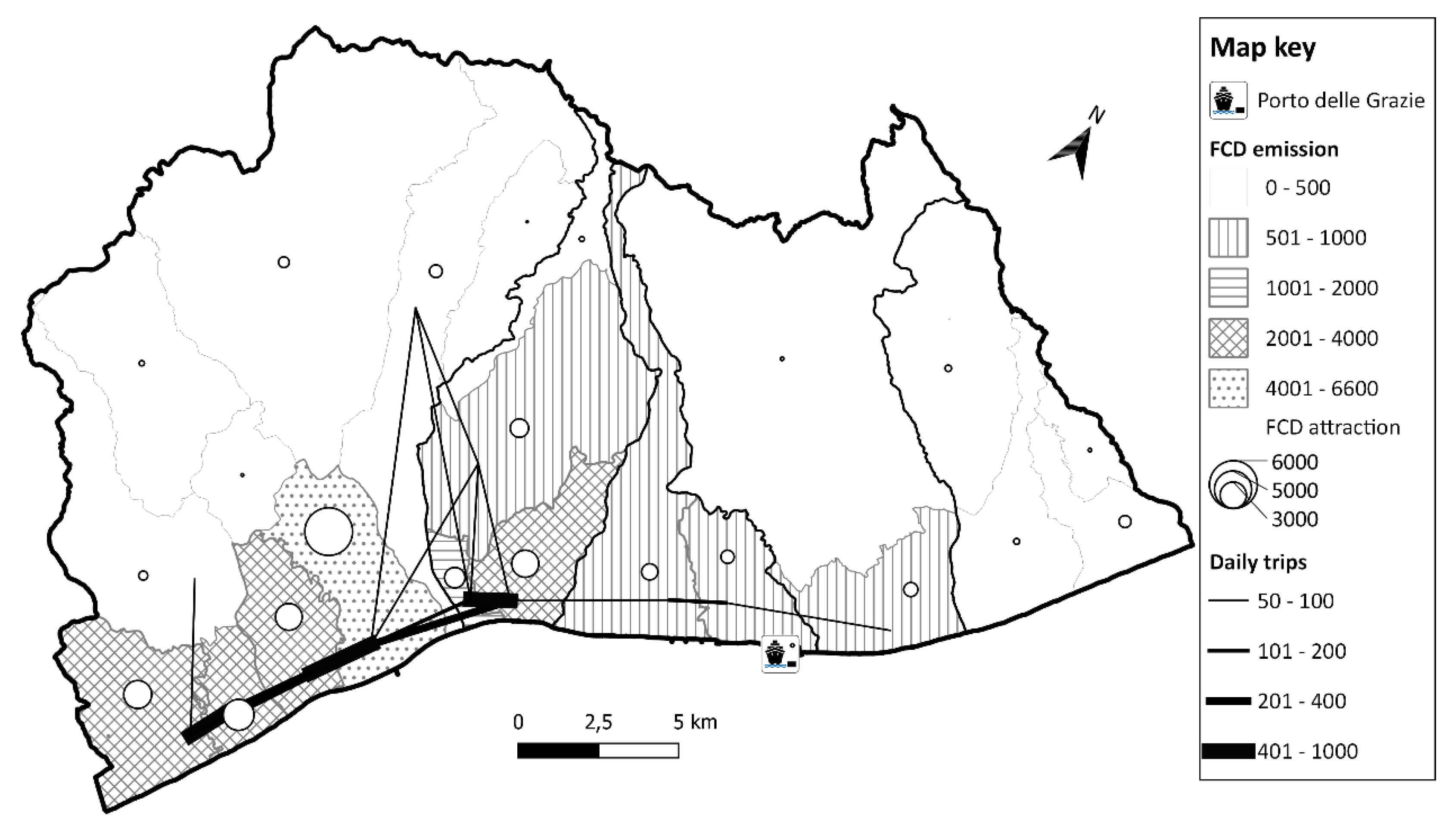
Figure 9 shows the relevant values (more than 50 trips/day) of daily generated/attracted trips and origin–destination flows.

4.3. Model Estimations (Inferential Analyses)

At this stage of the research, models in the literature [26,27,28] are used to estimate travel demand. According to the assumptions introduced in Section 4, models estimate trip generation and distribution during an average workday.

The models’ parameters are calibrated according to a what-if approach by updating the initial parameters until they could adequately reproduce the observed trips (direct estimation [26]).

The parameters are updated by minimizing the difference between the estimated values of trips (model estimation) and the observed trips (direct estimation; Section 4.1).

4.3.1. Specification

(1)

Generation

The specification of the generation model (Equation (4)) used for the experiment is a model where the number of generated trips from zone o of the study area for purposes s on a day (h = day) is obtained as follows (more details about the model specification are reported in [26]):

d(osh) = β_G,_sh * x_os

(12)

The initial values of the parameters, β_G,_sh [26], the average number of trips for each vehicle, of the generation model of (12) are presented in

Table 2. Initial values of generation model.

Purpose (s)	βG,sh	xos
C-L	0.17	Employees of zone o
C-Sc	0.14	High school Students of zone o
C-AM	0.15	Families number of zone o

.

(2)

Distribution

The specification of the distribution model (Equation (5)) used for the experiment is gravitational (more details about the model specification are reported in [26]), where the percentages of trips from zone o to zone d are calculated in relation to purpose s in a day (h = day):

$$p(\mathrm{d}|\mathrm{osh})=\frac{{\left({\mathrm{X}}_{\mathrm{A},\mathrm{d}}^{}\right)}^{{\mathsf{\beta }}_{\mathrm{D}1}^{\mathrm{s}}}\ast {\left({\mathrm{X}}_{\mathrm{C},\mathrm{od}}^{}\right)}^{{\mathsf{\beta }}_{\mathrm{D}2}^{\mathrm{s}}}}{{{\displaystyle \sum }}_{1\dots n}^{}\left[{\left({\mathrm{X}}_{\mathrm{A},\mathrm{d}}^{}\right)}^{{\mathsf{\beta }}_{\mathrm{D}1}^{\mathrm{s}}}\ast {\left({\mathrm{X}}_{\mathrm{C},\mathrm{od}}^{}\right)}^{{\mathsf{\beta }}_{\mathrm{D}2}^{\mathrm{s}}}\right]}$$

(13)

The initial vector of the parameters, β_D [26], of distribution model (13) is presented in

Table 3. Initial values of the distribution model.

Purpose (s)	βsD1	βsD2	XA,d	XC,od
C-L	0.93	−0.58	Public employees of zone d	Employees of zone o
C-Sc	1.00	−0.35	High school places of zone d	High school Students of zone o
C-AM	1.61	2.54	Trade employees of zone d	Families number of zone o

. The application of distribution model (13) allows for estimating the values of the distribution matrix, d(odsh), and therefore the vector of the attracted trips, d(dsh).

4.3.2. Calibration and Validation

In the case of the generation model, the parameters are different according to the classification of the origin zone, introduced at the beginning of Section 4, with no information on trip purpose [26].

In the case of the distribution model, the parameters are different for each trip purpose but are constrained to the same percentage variation from the initial to the updated values.

Five independent parameters are updated:

• two parameters of the generation model, one for each class of zone (Section 4);
• three parameters of the distribution model, one for each purpose, that are bounded to have the same percentage variation from the initial values.

According to Section 3.3.2, the parameters’ update of the generation-distribution models of (12) and (13) is conducted by building a constrained objective function (11) composed as the sum of three terms:

• sum of the quadratic difference between estimated trips with generation model (12), d(oh), and observed trips with direct estimation (1), d*(oh);
• sum of the quadratic difference between estimated trips with distribution model (13), d(odh), and observed trips with direct estimation (2), d*(odh); and
• sum of the quadratic difference between attraction trips estimated with (7), d(dh), and observed trips with direct estimation (3), d*(dh).

Each term is multiplied by a weight w_I (with I = I, II, III). The values of w_I, w_II, and w_III are, respectively, the weights of the generation, distribution, and attraction term of the objective function (11).

Table 4. Different configurations of the objective function (Equation (11)).

Model Specification	wI	wII	wIII	Generation	Distribution
Generation	x			x
Distribution		x			x
Attraction			x		x
Gen., Distr., Attr.	x	x	x	x	x

summarizes the tests performed, in relation to the type of FCD and to the term of the objective function that is activated by the values of the relative weights (w_I) different from 0.

Table 5. Calibration test results.

Test	Model Components	w			Objective Function	βopt/β (Optimal /Initial)					MSE	% diff.
		I	II	III		Generation		Distribution
						Class 1	Class 2	C-L	C-Sc	C-AM
0	Initial model	1	1	1	136,677,822	-	-	-	-	-	5,942,514	-
1	Generation	1	0	0	77,449,914	1.236	0.343	-	-	-	3,367,388	−43.33%
2	Distribution	0	1	0	115,416,313	-	-	0.803	2.090	1.169	5,018,101	−15.56%
3	Attraction	0	0	1	78,579,204	1.497	0.000	0.749	0.718	1.158	3,416,487	−42.51%
4	Gen, Distr, Attr.	0	1	1	61,545,785	1.416	0.162	0.752	0.832	1.825	2,675,904	−54.97%
5	Gen., Distr, Attr.	1	1	1	55,050,352	1.273	0.327	0.785	0.895	1.958	2,393,494	−59.72%
6	Gen., Distr, Attr.	2	1	1	55,114,670	1.258	0.337	0.789	0.901	1.975	2,396,290	−59.68%
7	Gen., Distr, Attr.	1	2	1	55,489,660	1.287	0.313	0.794	0.916	2.175	2,412,594	−59.40%
8	Gen., Distr, Attr.	1	1	2	55,884,681	1.287	0.321	0.771	0.873	1.540	2,429,769	−59.11%

shows the results of the parameters’ update conducted from the initial application of generation-distribution models (Equations (11) and (12)) with the parameters in the literature (Table 4 and Table 5).

Several calibration tests are conducted by assigning different values to the weights (w_I = 0, 1, 2) of each term of the objective function. The different configurations of weights are evaluated by using the statistical indicator MSE defined in (10).

The first row of Table 5 (test 0) contains the initial value of the objective function calculated by assigning to each weight w_I = 1. Tests 1, 2, and 3 are executed by considering separately each of the three terms in the objective function, and not considering the contribution of the other two ones. For example, in test n. 1, only the generation term is considered (w_I = 1), and distribution and attraction terms are not included (w_II = w_III = 0).

The last column on the right of Table 5 shows the percentage differences of MSE in relation to the initial values of the parameters. The optimal configuration of weights, which presents the highest reduction of MSE (−59.72%) obtained in test 5, considers the three terms of the objective function (w_I = w_II = w_III = 1). The ratios between the optimal and initial values of parameters, β^opt/β, show an increase in the generation parameter (1.273) of the zones in class 1, which are the zones near the coastline and with a higher population, and a significant decrease in the generation parameter (0.327) of the zones in class 2. The parameters of the distribution models slightly decrease for the systematic purposes (0.785, 0.895) and increase for the other purposes (1.958).

5. Conclusions

The general objective of the research is the integration of big data and traditional data in building the parts of TSMs related to travel demand models, to increase the capacity of transport analysts and planners to analyze, forecast, and plan mobility.

Data obtained from ICT tools are a precious source of information on TS; however, they allow the observation of historical and current TS configurations and to forecast its future configurations, in absence of exogenous non-systematic disturbances.

To obtain forecasts of mobility patterns, it is necessary to specify, calibrate, and validate TSMs. The building protocols of TSMs are based, essentially, on traditional surveys of a small sample of a population.

The contribution of this paper is the integration of the parts of TSMs related to travel demand and FCD, to support the estimation of the OD flow matrix. A framework to estimate travel demand, focused on trip generation and trip distribution models, inside an ITS, has been proposed. The demand models presented in the paper have been developed inside the LAST Lab of Università Mediterranea di Reggio Calabria. They are currently at the stage of research-oriented prototypes. No existing commercial transport tools can be directly applied for carrying out the research presented. The application is a real experiment to analyze the current (and future) passenger mobility in a sub-regional area located in south Italy. The results of the experiment are regarding the combined use of traditional data and FCD to do the following:

(1)

estimate observed generated trips and observed OD flow matrix in the study area (direct estimation); and

(2)

update the parameters of generation and distribution models (inferential analysis).

The following considerations can be drawn from this research:

• The context of the research is territorial areas characterized by a scarcity of monitoring technologies of the TS system (e.g., vehicle flows). Furthermore, also to limit the costs associated with the design and implementation of traditional surveys, commercial FCDs were used, which offer information limited only to space–time positions of road vehicles.
• The built travel demand model and the results obtained represent the potential use of FCD to obtain reliable estimates and forecasts of travel demand flows (Figure 1). The framework presented attempts to maximize the estimation capabilities of traditional (multi-step) travel demand models, for the generation and distribution levels, through the integration of traditional data and FCD, starting from available parameters previously calibrated for other similar territorial realities.
• Each problem requires a tailored solution in relation to the available data and cannot be solved in relation to the desired data. Traffic data can be obtained from several types of sources. In some cases, such as the specific context of the paper, a traffic monitoring system is not available, or the traffic data provided are not made public. Therefore, FCD are the only source available to obtain low-cost traffic data in a short time, considering that today, several vehicles have embedded GPS.

The authors propose a framework to be applied in territorial areas with the poor availability of traffic data. Additionally, areas with poor resources require procedures for solving problems. The framework could bring benefits for some classes of stakeholders involved in sustainable urban planning. For instance, public administration authorities could benefit from the use of the modeling approach to support transport planning via the quantitative estimation of some sustainable indicators; urban traffic systems operators could adopt the approach in order to quantify market mobility and, then, to define specific strategies.

The FCD adopted for estimating travel demand models has the following limitations.

The first limitation is connected to the penetration rate. The parameters’ calibration of the generation-distribution models is executed with a FCD penetration rate of 2.0%, which seems to be acceptable in the case examined according to the literature [12,13,14]. According to these authors, the following elements emerge. The first element concerns the average speed (or in-vehicle time), that presents limited estimation errors, and the level of coverage of the links of the network, that is acceptable on roads with moderate traffic flows with FCD penetration rates of 2.0%. The second element concerns the average error of vehicles’ spatial position provided by GPS, that is negligible in relation to the spatial extension of traffic zones. The assumption that the sample of vehicles traced with FCD is normally distributed across the fleet of circulating vehicles may hold because of the ubiquity of on-board GPSs. According to [35], the diffusion of smartphones in the population will increase worldwide, with a forecasted number of smartphone subscriptions from 2016 to 2026 passing from 3.668 billion to 7.516 billion. Therefore, it is expected that the penetration rate of probe vehicles in the traffic flow will increase in the next future, allowing to obtain more data for traffic analysis and estimation. It is worth noting that the availability of traffic data not only depends on the devices’ penetration in the population, but also in the people’s willingness to share their data [36].

The second limitation is that commercial FCD provide information related to road vehicles, not to users, not to the purpose. Therefore, some information related to users’ behaviour, such as trip purpose, is missing. FCD provide information related to road mode; and no elements are available concerning other transport modes (e.g., transit). The results of the application are valid because transit modes are not present as alternatives for transport users’ in the examined study area.

Considering the limits connected to the lack of traffic monitoring systems and to the limited information of the available FCD, the method proposed in this paper has good applicability in specific scenarios, and the results have a good guiding role for medium and long-term transportation planning. Transport planning depends also in journey patterns that could change in the time and in relation to the trip purposes adopting calibrated TSMs [37].

To support short-term planning, it is necessary to design and implement a traffic monitoring system able to continuously, and even in real time, provide traffic data [38,39].

A recent study [40] presented a method for error mitigation of the demand estimations from big data. The method proposed in this paper also aims to reduce the estimation errors, because it integrates traditional data and FCD to improve TMSs’ accuracy. The method is useful in specific contexts where there is a scarcity of available traffic and mobility data.

Further research will be conducted to overcome the identified limitations. Regarding the penetration rate, sensitivity analysis to assess the accuracy of the model parameters’ estimation will be conducted, based on the different values of FCD penetration rates.

Regarding TSM building, calibration will be extended in further research on travel demand model components by simulating additional dimension choices (e.g., purpose) and combining commercial FCD with other types of big data, or with survey data. The proposed methodology can be extended to other transport modes.

If applied in more technologically advanced areas, the proposed framework could allow for enhancing the estimates’ accuracy of the different components of the TSM. For example, an advanced traffic monitoring system (providing continuous data on vehicular flows and speeds) could provide data for the estimation of link cost functions, or of link speed-density diagrams [41], and through the implementation of reverse assignment models [42]. In this case, it will be possible to support the building of an info mobility system, with information for users on the current (and forecasted in the short term) status of the TS in real time, as well as short-term planning operated by public and private decision-makers.