Abstract
We present a new urban transit investment model, integrating transport economic theory regarding optimal investment with transport modeling, planning, and network design. The model expands on the theory of optimal transit network planning and investment, accounting for the effects of the investment on accessibility, level of service, and speed. The model seeks long-term optimal transit investment and optimal road pricing simultaneously in an integrated, unified model. To illustrate the advantages of our approach, we applied our empirical model to two case studies, Tel Aviv and Toronto, integrating our theoretical contribution into practice. Our results demonstrate the model’s ability to indicate the optimal transit mode and investment on a corridor level and the total investment required for the city transit network. The model results were compared to the actual and planned transit networks of Tel Aviv and Toronto and showed the model’s capability to produce a good balance of strategic design and network details. The research concludes that applying the right toll with the applicable transit investment is crucial for obtaining an efficient network and performance. This research can direct planners and policymakers in planning urban transport and provide a comprehensive set of guidelines for optimizing the simultaneous investment in mass transit and the congestion toll toward more sustainable cities and transportation systems.
1. Introduction
Mobility is essential and a major concern in cities all over the world. As population densities rise worldwide, urban mobility is increasingly becoming more complex to plan, regulate, and budget. Limited land and budget resources, growing traffic demand, and congestion make city transport planning crucial to enable accessibility, quality of life, and economic growth. This is a challenging task as not only do private vehicles have many negative externalities [1], but today’s planning and evaluation tools are biased toward investments in roads [2]. This paper develops and suggests a new urban transit investment model toward optimizing investments in public transport, the fundamental motorized sustainable transportation mode which enables more walkable and sustainable cities.
Vivier et al. [3] showed that, on average, public transport consumes four times less energy per passenger-km than a car. Nonetheless, in many cities, growing traffic congestion on roads and highways has led to increased investments in car-oriented infrastructure, with only a limited number of cities investing in public transport systems. The variation between cities and countries in public transport investment is large. Sharav and Shiftan [4] compared investments in public transport infrastructure in cities around the world and found that the average investment in public transport in Western European cities was USD 15 thousand per capita compared to an average of only USD 8 thousand per capita in developed cities. Vivier et al. [3] showed that Western European cities and some Asian cities developed mobility that is based more on public transport, they developed three to four times more public transport in exclusive right-of-ways than the motorways, and as a result, achieved high levels of public transport and non-motorized modes of usage (50–60%).
Cities vary in size, density, urban structure, population, employment, and other socioeconomic characteristics. These differences are also reflected in the transport characteristics and the mobility solutions that cities develop. City planners and decision makers need to choose which projects to build and how to allocate the budget among different types of transport investments. Moreover, cities that want to invest in public transport need to decide on the network structure, transit lines, and modes. However, planning the optimal transit network is a complex problem that has challenged many researchers. Among the prominent difficulties are the multiple criteria and fundamental uncertainties [5] and the choice of appropriate technology [6], where the large overlap between transit technologies in terms of generalized costs makes the selection of transit technology a difficult task [7,8]. In addition, there are caveats of the standard micro-economic appraisal of transit [9], and the mathematical complexity being an NP-Hard problem requiring heuristic approaches [10,11].
A typical urban transit planning procedure is a three-stage process: first, alternatives to the transportation network are designed; next, the alternatives are coded into the transport demand model, and the model is run to estimate the demand; third, an economic appraisal of the alternatives is conducted. These three stages can benefit the planning process, as feedbacks from the model and the economic appraisal are used to guide network design. However, there are major limitations to this routine procedure. First, the planner may miss important alternatives or links in the network structure since he only views feedbacks for planned alternatives. The transportation demand model, as well as the economic appraisal procedure, requires specific alternatives to perform traffic assignments, simulations, and analyses. Thus, the entire process is limited to inputs from the planner. While this allows determining the economic justification for specific alternatives, it is unsuitable for determining the optimal investment or the optimal network structure. Second, this three-stage process cannot direct planner decisions concerning the optimal transport mode and the investment at each transport corridor or identify missing links and lines in the plan. Third, these three stages run sequentially and separately, where feedback from later stages to earlier stages is limited.
This paper advances the theoretical and practical understanding of urban transport planning and investment to better facilitate transit planning and identify the required levels of investments in public transport and thus contribute to more sustainable transportation in medium to large cities. In this paper, we present an optimal urban transit investment model, integrating transit planning and economics into one unified model. The theoretical model is an extension of the model presented by Basso and Jara-Diaz [12], with the additional parameters of transit and road investment. Unlike the three-stage approach described above, our model is not limited to a specified set of predefined alternatives, and thus, the model can direct planners to the optimal transport network structure. We then apply the model in two cities, Tel Aviv, Israel, and Toronto, Canada, and demonstrate how the model can assist in planning and investing in the city’s transit network.
The rest of the paper is organized as follows. Section 2 provides a theoretical background on urban transport planning and investments and optimal public transport network planning. Section 3 describes the theoretical model and presents the case studies of Tel Aviv and Toronto. Section 4 presents the model results and analysis. Section 5 concludes the research and suggests how this research can assist transport planning and budgeting.
2. Literature Review
The literature review is constructed along the following sub-fields of transport system design. We first start with a review of the microeconomic approach of transport project appraisal, which is used to decide if a given project is beneficial and is commonly used to guide project-level decisions. We then cover the macroeconomic approach, showing the impact of transport investment on the economy, usually on the impact of a transport project or investments on the gross domestic product (GDP), the labor market, or the real estate market, which also assists the transportation planner in designing and selecting alternatives. These approaches are project-dependent, meaning that they can assess the impact of a given project or plan but do not provide any insight on the optimal network and investment. The micro and macro approaches are followed by yard-stick approaches to evaluate the need for transport systems such as metros, which are also a prevalent practice in mass transit appraisal, and can show the need for investment in transportation infrastructure at large. Next, the review shows recent urban transport economic models of optimal urban public transport systems (as opposed to project-specific appraisal), which this paper builds on. Fourth, we review the recent literature on transit design, as this paper deals with optimal transit systems on the empirical side, along with the theoretical side. We then conclude the review with the research of transit network analysis, which is used to analyze the optimal mass transit system, and compare it to other alternatives
2.1. Economic Appraisal of Given Transportation Projects and Yardstick Approaches
The microeconomic theory of transport investment was developed over 50 years ago, with the fundamentals of welfare theory as the basis for a Cost-Benefit Analysis (CBA). Theoretical developments have brought the project-level economic appraisal theory to its current practice [13]. These developments included the integration of macro-economic level analysis into micro-level CBA practice in the form of agglomeration effects and other wider economic impacts [14,15,16,17,18,19]. The resulting economic appraisal theory is now in common use in many countries as a practical method for transport project appraisal [2,20,21,22,23,24]. Over the last decades, the CBA approach has been the most dominant procedure for the evaluation of transportation projects. Martens [25] suggested a different approach, incorporating principles of social justice into the planning and evaluation procedure, as CBA does not provide insight into the accessibility shortfalls of particular population groups. Along similar lines, Nahmias-Biran and Shiftan [26] used activity-based modeling to introduce accessibility gains into a procedure similar to CBA, using individuals’ accessibility rather than time savings.
The macroeconomic approach of transport investments usually identifies the impact of a transport investment on the gross domestic product (GDP), the labor market, or the real estate market [27,28,29]. The extensive body of literature based on this approach demonstrated a large variation in the results and magnitudes of the estimated impacts. Berechman [13] showed that the output elasticity results from various macro-level studies in the U.S., Canada, and Japan were in the range of 0.03 to 0.56. The macroeconomic approach typically involves modeling (for example, using the production function model) to determine investments’ effects on the economy. As in the microeconomic approach, the macro-economic approach does not seek optimal investment but rather estimates the effects of a given investment/project.
Some researchers used the yardstick approach to indicate the need for transportation. Allport [30] and Loo and Cheng [31] showed that the yardsticks of 5.0 million habitants and USD 11,400 GDP per capita should be used to consider metro lines as a major part of the network. Sharav and Shiftan [4] found that over time the investment in public transport infrastructure increases public transport network average speed logarithmically, from 15 km/h in cities with low investments in public transport and no exclusive right-of-way, up to about 35 km/h in cities with developed metro systems. This research also demonstrated that cities that improved public transport supply over a long period of time and managed the demand for mobility have shown strong growth in public transport usage and modal share. In general, cities with higher urban density have a higher rate of public transport, cycling, and walking trips and are more efficient in terms of the total mobility costs [3,32,33]. Additionally, Vivier et al. [3] showed that on average public transport consumes four times less energy per passenger-km than transport by car. Public transportation also promotes other sustainable modes, such as walking and cycling, associated with health and environmental benefits, along with transportation benefits, which also indicates the need for public transportation [34,35,36].
2.2. Optimal Transport Systems
Designing optimal urban public transport systems is highly complex, and requires optimal network structure as well as optimal line design, line technology, vehicle size, and line frequency. Early public transport models mostly examined the level of service and the users’ and operators’ generalized costs, resulting in an optimal policy of line frequency, vehicle size, fare policy, and subsidy needed by the operators to maintain efficient levels of service [18,37]. In recent years, optimal transit design evolved to city-level networks with different urban structures and network representations [11,38]. Chen et al. [39] formulated continuum approximation optimization models to design city-wide transit systems (ring-radial or grid) at minimum cost. Fielbaum et al. [11] presented a model aiming to find the best line structures for urban public transport, using an urban structure of one CBD and in surrounding sub-centers. Saidi et al. [40] developed an analytical model aimed at identifying the optimal number of radial and ring lines in a city. Zhao et al. [41] developed a model that examined the scale of urban rail networks given the population. Lee and Vuchic [42] developed an iterative model to plan the optimal transit network, with variable transit demand and under a given fixed total demand. Basso and Jara-Diaz [12] developed a bimodal model where congestion toll, the transit fare, and transit frequency optimize social welfare. Additional models were presented by Baaj and Mahmassani, Börjesson et al., Ceder and Yechezekel, Jara-Diaz et al., Beaudoin et al., Tirachini et al., and Tirachini and Hensher [43,44,45,46,47,48,49]. As for automated transit systems, research in recent years investigated the optimal capacity of automated rail-bound transit [50] and the effect of automated public transit on cost, fare, and subsidy [51].
The interdependency between transportation and the urban economy has been developed by Anas [52]. Anas [52] explored the optimal pricing, finance, and supply of urban public transport and roads, and reported that highly populated cities are characterized by increased core land rent and increased congestion. He also showed that the investment in roads should equal the total toll revenues collected from car users, while the investment in public transportation should equal the price gap between land rent in the city’s core and the nearby suburbs. Anas’ research includes optimal investment in public transportation in a core-periphery model, as such, it does not specify the optimal investment in a corridor resolution.
2.3. Network Design
Recent work has also concentrated on the economic effects of transit line structure design, with a focus on urban bus lines in the short to the medium time range. Fielbaum et al. [53] studied how the spatial arrangement of transit lines influences scale economies in public transport, emphasizing the importance of directness, an element that encompasses the number of transfers, number of stops, and passenger route lengths. The same authors have incorporated spacing of transit lines, frequencies, vehicle sizes, and routes in the design and the analysis of scale economies in transit systems, showing, among other results, that considering spatial spacing as a design variable in transit network can increase the effect of scale economies [54]. Other considerations of line structure design include integrating existing bus and metro networks into a single connected transit network to increase connectivity [55], equity outcomes of transit network design with distance-based fares [56], the effect of ride-pooling on transit network design [57], and the design of a bus transit network where there is an existing metro network that can balance the modal split between metro and bus [58].
2.4. Transit Network Analysis
Complex network theory and analysis have become an important component of many transit network planning methodologies. Lin and Ban [59] reviewed recent work in transportation network analysis and discusses some case studies that used graph theory and measures. Levinson [60] used network indicators, such as connectivity, treeness, circuity accessibility, and entropy, to study network structure in 50 large US cities. His research suggested that larger cities are more connected but have less capacity per capita as well as longer commute times. Derrible and Kennedy [61] analyzed metro networks in cities around the world using an updated graph theory. Derrible and Kennedy [62] presented metro systems development phases (“State”) on a graph, showing connectivity and complexity. Sharav et al. [63] compared network indicators of combined metro and light rail mass transit systems.
The contribution of this paper is twofold. First, it further develops the theoretical model of Basso & Jara-Diaz [12] to include, among optimal congestion pricing and transit subsidies, also optimal transit investment. Second, and most importantly, this paper presents an empirical model which integrates short and long-term transport policy decisions, applicable to any city on a corridor level, determining the short-term optimal congestion pricing, transit subsidies, and long-term transit investment, on every corridor. Thus, the empirical model can help policymakers and transport planners detect the optimal transit network design for their city when building a new mass transit system or expanding an existing one, along with the optimal congestion pricing, transit subsidy, and transit frequency, bridging the gap between theoretical optimal design and current practice.
3. Materials and Methods
The methodology includes three major modules. First, we developed a theoretical urban transport model, based on microeconomic welfare theory. This theoretical model aims to find the optimal investment, optimal road pricing (toll), and optimal transit fare and frequency in an integrated two-mode setup. Second, an empirical model was developed using the theoretical model’s results applied to the city on a corridor level. The empirical model aims to find optimal transit investment and optimal transit mode on each corridor. The total optimal investment in the city’s transit network can then be derived by summing the investments of each transit mode on each corridor. Lastly, we applied the empirical model to our case study cities: Tel Aviv and Toronto. In this last step, we calibrated and applied the model taking into account the unique features of each city. This is a major effort. It was important for us to demonstrate it in two cities such as Toronto, which has a metro system to compare with its network, and then apply it to Tel-Aviv, which currently planning a metro. We then analyzed the models’ outputs of optimal investment, transit mode, and network structure. Finally, we compared these results to the current and planned transit networks of these cities and draw conclusions showing how the model can best be applied as an integrated tool assisting planning and policy decisions.
3.1. The Theoretical Model
The theoretical model aims to find the optimal investment and the optimal transit mode for each corridor in the city. The model also integrates short-term policy decision parameters—such as road pricing (toll) and transit fares and frequency. We set the peak hour demand of X passengers that commute by auto or by transit. Let XA and XT be the demand for auto trips (both drivers and passengers) and transit trips, respectively. We set the generalized user cost function for each mode similarly to Basso and Jara-Diaz [12] with new parameters of transit investment (IT) and road investment (IA). The investment affects transit and road speeds, as described in Equations (1) and (2):
The model includes time cost, operating cost, transit capital investment, transit fare, and optional road pricing (tolls or parking fees). Transit time cost includes both vehicle travel time and waits time in the station.
Road network congestion is described by the assumption that,
We set the total transit in-vehicle travel time as:
where,
- gA = auto user generalized cost;
- gT = transit user generalized cost;
- PA = auto road price (toll);
- PT = transit fare;
- ACA = average cost for auto drivers;
- OCA = auto operating cost;
- α = value of time (VOT);
- IA = investment in roads;
- IT = investment in transit;
- ACTU = average cost for the transit user;
- f = transit frequency, departures per hour;
- TA = auto travel time;
- TT = in-vehicle transit travel time, including delays caused by other transit passengers;
- Tm = transit travel time without delays caused by other transit users;
- β = ratio of out of vehicle VOT to in-vehicle VOT;
- µ = in vehicle delay caused by other transit users boarding the vehicle;
- X = number of trips (workers or city commuters);
- XA = auto trips demand (driver and passenger);
- XT = transit trips demand.
Note: All costs are in 2015 US dollars. All the time parameters are in hours. Demand data is person trips per hour.
To keep the model robust, we included only direct operating costs, time costs, and congestion costs. Other costs or benefits, such as road safety and environment externalities, wider economic impacts, and reliability, are not included in this version of the model but might be included in future model developments.
We assume a general mode choice model, H, (such as the Logit model), and for the two modes model:
We can now define the objective function of the theoretical model maximizing the total social welfare, including the consumer surplus, road toll revenue, transit revenue, and operating and investment cost:
We are looking for the long-term optimal transport investment policy (IT and IA), along with short-term policy parameters of transit frequency f, and prices (PA and PT) that will maximize the social welfare in terms of the total sum to all individuals.
This research focuses on the optimal transit investment IT while keeping the road capacity and investment fixed (IA). Further extensions could also incorporate the effects of road investment in the integrated system.
where k is the vehicle capacity.
The mathematical analysis is described in Appendix A—Theoretical analysis. From the first-order condition, the partial derivatives of W by PA and PT, we obtain:
That implies that, in equilibrium, the price gap between the road toll and transit fare equals to:
The partial derivative of W by f gives:
From that, we obtain the optimal frequency as:
We assumed C(IT)f is a logarithmic function C(IT)f = bln(IT) + d (see Appendix A and Appendix C, Figure A2).
The partial derivative of W by IT with the results of Equation (6) produces the optimal transit investment policy as:
Sharav and Shiftan [4] showed that higher investments in public transport increase transit speed logarithmically—from an average of 15 km/h in cities that invested little in public transport up to 35 km/h in cities that invested heavily in mass transit.
As presented by Sharav and Shiftan [4], Tm as a function of IT can be described as:
Therefore, the condition in Equation (8) is as shown in Equation (9):
Examining the expressions obtained for IT, we find that the a < 0 transit investment IT increases with the number of transit passengers, XT, and the value of time, α.
3.2. The Empirical Model
The theoretical model produces an equilibrium in a two-mode setting. Figure 1 illustrates the combined auto and transit optimal equilibrium on one corridor with total demand of X passengers. The marginal cost equilibrium is at the point E1 where MCT = MCA. Point E2 represents the average cost equilibrium (ACA = ACT) in the absence of road tolls and subsidies. At the marginal cost equilibrium, E1, X*T passengers use transit, and X*A = XX*T use auto. The model allows calculating the optimal investment at the equilibrium E1 according to Equations (6)–(10). We can then calculate the optimal transit investment I*T in the corridor as derived from Equation (11).
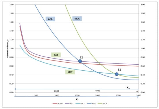
Figure 1.
Auto trips and costs are presented from right to left, and transit trips and costs are presented from left to right (X = XA + XT = 3000).
The model calculates the optimal investment based on the corridor characteristics, the generalized cost functions, and the demand on the corridor. If the model shows that passengers are less willing to choose transit in that corridor (less than the optimal level, presented as X2T < X*T), then we can calculate the applicable road pricing (toll) PA that is needed to obtain the optimal level of the car and transit usage corresponding with the optimal investment: PA = MCA(X2A) ACA(X2A). A particular example is the average cost equilibrium, where users face no toll, and hence, more passengers choose a car. In this case, applying road toll will shift passengers to transit, and the more efficient system equilibrium at E1 can be obtained.
The empirical model application uses a similar calculation on a multi-corridor level and is set on a TransCAD platform. For this purpose, the city is divided into super zones. Each super-zone is connected to its neighboring zones by a virtual corridor in a spider web network. Each corridor is represented by a single bi-directional road and is serviced by bus service with a minimum frequency of two trips per hour. The model assigns the demand between all pairs of origin-destination zones on the corridors and calculates the level of service and modal split. Model iterations between the assignment and modal split continue until the model split converges.
Following convergence, the marginal cost equilibrium and the applicable optimal transit investment and mode on each corridor can be obtained using the generalized cost functions and the characteristics of the corridor as described in Equation (1) and the results presented in Equations (1)–(11). The empirical model points to the optimal investment and the applicable transit mode on each corridor. The model recalculates the level of service and the demand on each corridor simultaneously based on the new modes and thus takes into account the effect of the transit network.
The empirical model structure is presented in Figure 2.

Figure 2.
The empirical model structure.
The model provides a formula for calculating the optimal toll needed to achieve the marginal cost equilibrium that is also coherent with the optimal investment:
This theoretical result implies that the optimal road toll is obtained when passengers pay the difference between their marginal cost to their average cost for each road segment and the time of their trip.
3.3. Application of the Empirical Model
To investigate the model capabilities to help planners designing a city’s mass transit system, the empirical model was applied to two case studies—the cities of Tel Aviv and Toronto. The city of Tel Aviv does not have a mass transit system yet, while the city of Toronto already has a developed mass transit system. In the Tel Aviv case, we compared the model results to the future mass transit plan. In the Toronto case, we compared the model results to the existing mass transit network.
Tel Aviv was divided into super-zones based on the Tel Aviv Travel Demand Model (TTDM). Each super-zone is connected to its neighboring zones by a virtual corridor that represents all the roads and transit services between them. We focused on peak morning trips that are usually used to determine the transit system capacity and investment. For each super-zone, we used the TTDM population and employment data and forecasts, employment and population density, and the number of households by car ownership sub-groups.
The model is iterative where the model’s first run assumed that all corridors consist of two three-lane carriageways and a capacity of 1500 cars per lane. The capacity was then revised using TTDM results for the 2012 base year’s network by looking into the volume over capacity ratio on the roads connecting the super-zones. Using the Bureau of Public Roads (BPR) volume delay functions calibrated to Tel Aviv, we could calculate the model capacity for each corridor. We assumed that the 2012 capacity is not extended in the 2040 network.
The model assigned the demand on the corridors and calculated the level of service using the TransCAD software. The initial speed was set as 70 km/h for car passengers, and 0.9 times car speed for transit passengers, with a maximum of 15 km/h—representing an initial model state of basic bus services on all the corridors with no mass transit or busways (Average bus speed in Tel Aviv. See also Sharav and Shiftan [4] for average transit speeds in cities with no right-of-way). This initial transit setup allows the model to show the optimal transit investment and mode results regardless of the existing transit network, which can then be compared to the actual (or planned) mass transit network. The modal split model can then be used to calculate the number of passengers over the three modes: car driver (Single Occupancy Vehicle—SOV), car passenger (High Occupancy Vehicle—HOV), and transit. We used a simple Logit modal split model based on the TTDM with a few parameters representing a trip cost, trip time, number of cars per household (representing passengers’ characteristics), and job density in the destination (representing the city’s characteristics). We also included optional road pricing (toll) on the network (Appendix B—The modal split model).
The modal split model uses calculations of the level of service for each iteration, passengers’ distribution by car ownership (0, 1, or 2), car cost per km, and transit trip cost based on the transit fare matrix for each trip. Job density data is obtained from the TTDM. The model iterations continue until the model’s split converges. In each iteration, the level of service is calculated using BPR volume delay functions calibrated to Tel Aviv.
When the modal split model converged and the demand on the corridors is assigned, the model calculates the optimal investment for each corridor and the applicable transit mode. The investment is calculated for the peak direction demand and is then multiplied by two to represent that the same mode is chosen for both directions. This is an obvious assumption in the case of a metro, Light Rail Transit (LRT), or Bus Rapid Transit (BRT) but we also assume that busway is always bi-directional. The results of the optimal investment calculation and applicable optimal mode determine the new level of service on each corridor, and then the model calculates the new modal split.
3.4. Data Sources
3.4.1. Tel Aviv’s Demand Data
For the optimal investment model, we used demand data for the years 2012 (current) and 2040 (forecast), for the peak AM period (average hour: 6:00–9:00). The data for Tel Aviv was received in the form of origin–destination matrices representing passengers’ trips (motorized trips only) from the TTDM. The TTDM has 1200 zones in a four-ring formation. We used the inner three rings, aggregating the data according to the 31 super-zones representing the urban area of the city. Short inner zonal trips and walking and cycling trips were disregarded since, for the model’s objective of finding the optimal transit investment, only longer commute trips are relevant. External trips that are not within the urban area were also omitted.
Travel habits and modal split data were analyzed based on the Tel Aviv Travel Habit Survey 2014 (TTHS 2014). The survey included 35,952 daily trips in the metropolitan area.
The non-motorized modes (about 40% of all trips) were not included in the optimal investment model. Table 1 presents the summary demand for the peak AM period (6:00–9:00) from TTHS 2014.

Table 1.
Tel Aviv passenger trips to center and total, by mode.
3.4.2. Toronto’s Demand Data
Toronto’s demand data was based on the 2011 Transportation Tomorrow Survey (TTS) received from the University of Toronto. The TTS contained detailed demographic information for all members of each surveyed household, and a ledger of travel information for an entire weekday. Table 2 presents the summary demand for the peak AM period (6:00–9:00) from TTS 2011.
Table 2.
Toronto passenger trips to center and total, by mode.
3.4.3. Cost Data
All cost data are in 2015 US dollars. The transit capital investment costs and operating costs were estimated based on cost data for the Tel Aviv mass transit system [64], prepared by Egis [65]. The same unit costs were assumed for the Toronto transit network. Table A1 in Appendix B describes the capacity, maximum frequency, and the amortized investment cost for one peak hour for each transit mode.
Additional transit data analysis was conducted over the US National Transit Database (NTD). Car operating cost for both models was based on the variable cost of the average hybrid electric car representing current and the future marginal cost of private cars. The average car operating cost used in the model is USD 0.4/km and the marginal operating cost is USD 0.09/km (Source: https://www.nerdwallet.com/blog/loans/electric-hybrid-gas-how-they-compare-costs-2015/, accessed on 1 July 2021).
4. Results
4.1. Tel Aviv Network
The model was applied to the city of Tel Aviv for the current network (2012) and future network (2040). Figure 3 presents Tel Aviv’s 2040 mass transit plan, approved by the government of Israel in 2016 (TLV alternative C3). This plan includes two radial metro lines with six radial branches and an additional semi-circular metro line.
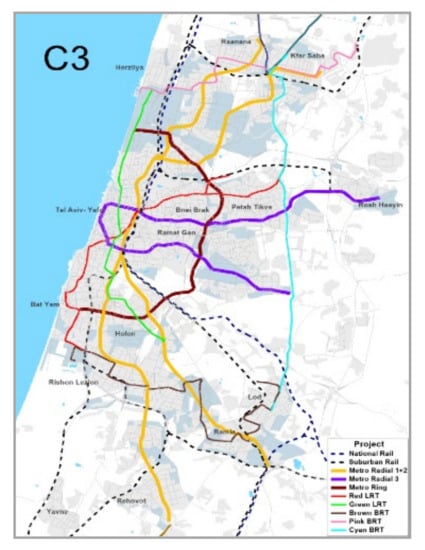
Figure 3.
Tel Aviv 2040 transit plan—TLV alternative C3.
Figure 4 presents the model’s results for the optimal transit investment and the applicable mode for 2040 (left panel), and transit volumes with optimal modes and optimal road pricing on each corridor for 2040 (right panel). The optimal transit investment for the city is calculated as a sum of the investments on all the corridors and is presented in Table 3. The model results for the year 2040 show that the optimal transit investment includes 11 metro corridors, 18 light rail corridors, and 29 BRT corridors. The total optimal transit investment is USD 14.8 billion—compared to USD 8.5 million in 2012. According to the model, the metro and light rail corridors should be increased significantly by 2040. Radial metro branches to the core should be increased from four to six. The future optimal results of non-radial metro branches indicate more clearly the need for a ring-shaped line.
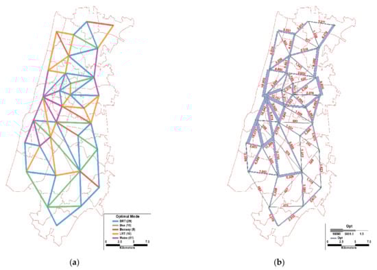
Figure 4.
Model results for Tel Aviv 2040—optimal investment, transit modes, and transit volumes (peak hour) with optimal road pricing. (a): Optimal transit modes. (b): Transit volumes with optimal mode.
Table 3.
Optimal transit investment and mode for Tel Aviv’s current (2012) and future (2040) network.
Table 4 presents transit share for trips between metropolitan rings before and after applying the optimal investment model for the 2040 demand forecast. Ring 1 represents the core of the metropolitan area and ring 3, the outer ring about fifteen kilometers from the center. The results show that the optimal investment introduced by the model increases transit usage from 24% to 30%. The radial trips from rings 2 and 3 to ring 1 have the most increase. The optimal toll result in the model was applied only on trips to ring 1. The results show that transit share increased to 33% and that trips to ring 1 increased from 47% to 58%.
Table 4.
The effect of optimal transit investment and toll on transit share between metropolitan rings.
It should be noted that the model provides the optimal mode for each corridor. This is a tool for the planner to design specific projects. The planner, knowing which mode is optimal for each corridor, can design the lines and specific projects based on this output. The actual network’s length and investment will probably differ from the model’s results due to two considerations. The first consideration is that the actual transit routes will most likely be longer than the straight lines represented in the model as corridors between super-zones. The second consideration is that the model shows the optimal investment on each corridor, but, in the actual plan, the planner should consider the continuity of the chosen technology all through the line. For example, if the model indicates that the optimal mode for corridor A is LRT, and metro on the continuing corridor B, the planner would conclude that the transit line on A and B should be metro all the way to reduce the operational complexity and the number of transfers, or the planner can decide that corridor A would be LRT feeding a metro line on corridor B. This example demonstrates the model results as a supportive planning tool, leaving some consideration to the planner’s decision, such as the overlapping range of cost and capacity of the different technologies. These considerations can be included in the model, but their inclusion will obstruct the optimality of the model’s results. Instead, the model’s results can be considered by the planner along with these considerations.
Comparing the results of our model for 2040 to Tel Aviv’s new mass transit 2040 plan (TLV alternative C3, Figure 3) reveals that the optimal investment in the model should be only indicative for the final plan solution.
4.2. Toronto Network
The Greater Toronto Area (GTA) is divided into 46 super zones. Our optimal transit investment model for Toronto was developed on a corridor network over the super-zones 1–36, representing the urban network. A spider web corridor network connecting all neighboring zones was defined, including some additional links between zones that do not have a common boundary but have a direct connection in the actual network. Such additional links in the spider web network are necessary since they follow transit lines or roads (for example, the Yonge metro line). The final spider network includes 54 links/corridors. As in the Tel Aviv model, the speed was set to 70 km/h for car passengers and 0.9 times the car speed for transit passengers with a maximum of 15 km/h, representing an initial state of basic bus service on all the corridors with no mass transit. This initial transit setup allows the model to show the optimal transit investment and mode results regardless of the existing transit network, which can be compared to the actual mass transit network (Figure 5).
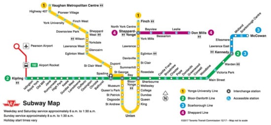
Figure 5.
Toronto’s metro network. Source: Toronto Transit Commission, 2017.
The model results for Toronto are shown in Table 5. The optimal transit investment and mode for Toronto’s current network were modelled. The results suggest that the optimal metro length for the Toronto transit network is 147 km and that the light rail optimal length is 31 km. In addition, more than 200 km of BRT and busways are needed. The total optimal investment was estimated at USD 39.8 billion, more than double that of the Tel Aviv 2040 network.
Table 5.
Optimal transit investment and mode for Toronto’s current network.
Toronto’s current metro network’s length is 74 km (Figure 6). Our results indicate that more metro lines are needed, and the total metro network’s length should be doubled. This conclusion is in line with the results of Derrible and Kennedy [66], who investigated Toronto’s metro network’s structure based on the updated graph theory.

Figure 6.
Model results—Toronto current network: optimal investment and mode.
Figure 6 presents the model results for the optimal investment and mode on each of the network’s corridors Figure 7 presents transit volumes’ forecasts on each corridor for the optimal network and level of service. The model indicates the need for four radial metro branches to the city center (from zones 2, 3, 4, and 6 to zone 1). In addition, the model indicates the need for at least one additional West–East line or a semi-circular line along Eglinton or 401 corridors, creating a spider web shape network. The lines in the existing network (Figure 5) are set in a different formation, with the Yonge–University U-shape line serving as two radial branches and the Bloor–Danforth line serving both as an East–West service to mid-town and a feeder to the Yonge–University line connecting to downtown Toronto. This structure can be regarded as a network of four radial branches, in line with our model’s suggestion, but using a less extensive metro network to achieve that. The model’s configuration will have better performance in terms of metro connectivity, level of service, and coverage, and will ease the congestion on the 401 highway and the radial roads. Again, our results are also supported by those of Derrible and Kennedy [66], as well as other plans for the future transit network in Toronto.

Figure 7.
Model results for Toronto’s current network—transit volumes in peak AM hour.
Multiple plans have been designed for Toronto’s future mass transit network. The city’s “relief line”—a new U-shape radial metro line to the center—is currently under planning. This line will add two more radial branches to the center as the optimal investment model suggests. The 15-year plan also presented the Eglinton metro line, a new West–East connection, as suggested by the optimal investment model. The new Eglinton line was planned as a metro line in some plans and as an LRT line in more recent plans. In contrast to these new plans, our results suggest that a metro would be optimal in this corridor. It is worth mentioning that some more ambitious plans for Toronto’s mass transit network are not presented here in detail. However, some of these plans included three West–East metro lines and three U-shape radial lines. The model’s results indicate the need for two or three West–East metro lines and four radial metro lines. In addition, six radial branches might be needed with future demand growth that was not part of this research. The model’s results showed heavy usage during peak hours on all four radial metro corridors.
Another interesting result of the model indicated the need to extend the University metro branch to the city of Vaughan (zone 33). This extension is currently under construction and is due to open in 2018. A metro connection between zones 10 and 11 seen on the optimal model was also suggested to be included in the future network. Indeed, this link appears in some of the future transit plans for the city. The Mississauga (zone 36) Brampton (zone 35) light rail project along the Hurontario corridor is in line with the model’s metro line for that corridor. The model’s results that more expensive technology is required can be explained by the size of the super-zones 35 and 36 in the model. Ideally, super zones should include one or two transportation corridors. However, in this case, the zones might be too big and thus the corridor in the model attracts more passengers (see discussion in further research). The model’s results for the Richmond Hill (zone 29) to zone 11 connections were expected to be optimal as a metro, as the current high passenger volumes on this Yonge metro line section implies. However, the lower result in the model can be explained by a few factors. First, the zones’ structure in this area might require a better definition. Zones 31 and 33 might divert some of the North–South traffic from the Yonge corridor to the East and the West. Second, our model does not consider external trips that might be coming from outside of the model’s zonal system. Some of these external trips might be using the Yonge line with park and ride and kiss and ride options.
A sensitivity analysis was carried to examine the model sensitivity to the value of time. The Toronto model results presented in Table 6 show that an increase of 10% in the passengers’ value of time increases the total network optimal investment by 3.7%, and an increase of 25% in the VOT showed an increase in the optimal investment by 14.8%. This result suggests that a higher value of time has more impact on the network investment.
Table 6.
Results of the value of time sensitivity analysis.
This result shows that the value of time has a very high impact on the optimal investment in the city. It suggests that when density exists and all other parameters are constants, a real increase in the value of time should increase the investment in public transportation. However, one must take into account that the value of time sensitivity result of this model is high because other externalities such as safety and environmental costs are not included in the model, giving more weight to the congestion time costs.
5. Conclusions
Transport economic theory deals with urban transport investments and planning using various approaches. Few researchers have addressed the question of how much should be invested in an urban public transport network, perhaps due to the complexity of the problem. However, some economic models relating to this question have been developed in recent years [47,52]. Moreover, the complexity of the problem has challenged many researchers to develop heuristic approaches to the planning of the optimal network in terms of structure, transit lines, and modes [10,11].
This research introduces a strategic design model that can direct planners and policymakers to high-level strategic questions. The model is built on a spider-web corridor network, and it is detailed enough to design a transit network structure without going into street-level details and complexity. Many of the city-level economic models are based on a schematic city structure, such as a core and suburbs [52] or a core and sub-centers [11]. Extending these models, our model is designed to produce corridor-level design results. As a result, the model can indicate the optimal number of mass transit lines as well as the shape and structure of the transit network with respect to the actual city land use, activities, and demand.
The model expands the theory of optimal transit network planning and investment, taking into account the effects of the investment on accessibility, level of service, and transit speed. It seeks optimal transit investment and road pricing simultaneously in an integrated, multi-modal model. Our method combines the two major approaches used to address congestion—giving priority to public transportation and road pricing—with one unified theory that addresses infrastructure investment and policy decisions simultaneously. To illustrate the advantages of our approach, we applied our empirical model to two case studies, integrating recent theoretical developments and our theoretical contribution in practice.
Our results demonstrate that the model can produce strategic-level answers to the questions of optimal network design and investment that can be further investigated with more detailed planning tools. The model corridor-level results for optimal investment and mode were compared to the actual and planned networks for both Tel Aviv and Toronto. The comparison shows the model’s capability to produce a good balance of strategic design and network details, that can assist planners with transit network design.
Finally, this model contributes to the emerging literature in Sustainability about the need to improve transit systems and their planning tools to promote sustainability [67,68,69,70,71,72,73,74].
6. Further Research
Our results demonstrate the model’s ability to indicate the optimal transit mode and investment on a corridor level and the total investment required in the transit network in the city. This approach integrates optimal investment from the transport economic theory with transport modeling, planning, and network design. The model results can be compared to the city’s current network and future transit plans and can provide insights on how to design better and more efficient transit networks and identify missing links in the networks and the optimal mode.
However, being a strategic decision tool, the level of detail should maintain a balance of the micro and macro levels to optimize the model results and achieve its objectives. Future research should focus on the following issues:
Objective function—In this research, our analysis focused on maximizing social welfare. It would be interesting to introduce different objective functions such as profit maximization. The profit-optimal investment strategy should be considered if a private firm would be set to invest in a mass transit line or network, however, given that transit is usually provided by the government, we focused on the maximum welfare case. In the profit maximization strategy, it might be obtained at higher service price and less transit riders.
Super-zones size—The size of the super-zones is a key element in the model’s ability to predict valuable results dictating the level of resolution. If the chosen size is too small, corridors will not concentrate enough transit passengers. If, on the other hand, the size is too big, corridors will have too much concentration and not enough population coverage. These requirements of the model suggest that zones should include at least one corridor to each of their neighboring zones and have good public transport coverage, so the corridors should cover most of the zones within one kilometer of walking distance.
Corridor capacity—corridor capacities are among the model’s parameters. Corridors can be assigned unique capacity values or can be assigned value according to the corridor’s type (by type of area, by the metropolitan ring, by population density, etc.). These capacities influence road congestion costs and thus also optimal road and transit equilibrium. Ideally, a corridor’s capacity should represent the affective capacities of all roads and intersections connecting the two super zones.
Corridor length—corridors’ lengths were set to the aerial distance between super zones’ centers. This measure is set as a default value in the model and aims to represent an average trip distance between zones. However, the trip length might be different in real life for many reasons such as the housing and activities’ location in the zone, the road layouts, and more. These considerations could be addressed in further research regarding the position of the zone center and introducing corridor length factors.
Access and egress time—The main feature of transit investment that is investigated in our model is the effect of transit investment on transit travel time and wait time from station to station. Investment in higher transit modes such as light rail or metro increases transit speed and decreases wait time. To simplify the model, access and egress time to the stations are not included. Future research should include access and egress time, along with non-motorized modes, to set a more holistic framework to sustainable mobility in the city.
Other modes—the model is based on three modes: car driver, car passenger, and transit. This choice is in line with the goal of finding the optimal transit investments for longer commute trips. Extending the model to include shorter trips can be accomplished by introducing non-motorized modes such as walking and cycling. In addition, the current model’s transit supply modes include four modes (bus, BRT, LRT, and metro). Other transit modes such as Personal Rapid Transit (PRT) can be incorporated into the model. To do so, operating and capital cost data, basic operational data, and passengers’ preferences data will be required. The model focuses on the main transit network, future work can expand it to complementary modes of walk and cycling which are essential to sustainable cities.
Autonomous Vehicles (AV)—autonomous vehicles, and especially shared autonomous vehicles and other transport services, could also be incorporated into the model. However, this will require additional data and assumptions. On top of the cost data, the model would need assumptions regarding passengers’ preferences, capacity, and trip generation effects (such as empty trips).
Cost components—to keep the model robust, we included only the direct operating costs and cost of time. Mackie et al. [75] showed the importance of travel time savings in project evaluation. Hensher [76] also concluded that the value of travel time savings is critical in project evaluation, typically accounting for 60% of the project’s benefits. Thus, the model includes time cost, operating cost, transit capital investment, transit fare, and optional road pricing (tolls or parking prices), while road externalities are represented by the congestion costs. Other externalities and costs, such as road safety and environment, wider economic impacts, and reliability, are not included in this version of the model and can be incorporated in future developments of the model. We estimated the value of time at USD 8 per hour. This compounded value of time is consistent with the Israeli guidelines for transportation projects analysis from 2015 as well as with the recommendation set by Mackie et al. [75]. Nonetheless, this crucial parameter can be adjusted for each city. The model can also be extended to include agglomeration benefits with an increase in job density attributed to the investment in the transit network and the effect on wages [16].
Day periods—peak morning trips are commonly used to determine the transit system’s capacity and investment. The current model focuses on this day period. However, other day periods could be easily incorporated to evaluate the daily performance and efficiency of the optimal investment determined by the peak period. The extension of the model to other day periods would require daily demand data.
Road investments—the empirical model aims to seek optimal transit investment assuming the road network is fixed. Further extension of the model can incorporate the effects of road investment on the integrated system.
Equity and fairness considerations—the theoretical model presented in this research uses an objective function derived from the utilitarian social welfare approach. The social welfare approach maximizes the sum of benefits while ignoring the distribution of benefits and costs among different members of society. Alternative social approaches have been discussed in the literature, such as Nash or Rawls [25,77,78,79]. An important extension of the model presented here will be to incorporate social justice theories and practices by examining individuals or groups and assigning them with a potential mobility index [25] or by utilizing a different objective function, for example, the Nash social welfare.
This study has gone some way towards a unified theory that addresses infrastructure investment and policy decisions simultaneously. Integrating transit planning, transport economics, and policy decision making, we aimed to identify long-term optimal transit investment policy while optimizing short-term decisions. As a strategic decision tool, the model aims at maintaining a balance between the micro and macro approaches. This critical balance, along with other issues, should be further considered in future studies. Specifically, to better contribute to sustainability, future work should extend the model to account for all externalities including environmental, safety, land consumption, and more, as well as cycling and walking.
Author Contributions
Conceptualization and methodology—both authors; analysis, investigation, resources, data curation, and writing—original draft and preparation—N.S.; review and editing—Y.S.; visualization—N.S.; supervision—Y.S. Both authors have read and agreed to the published version of the manuscript.All authors have read and agreed to the published version of the manuscript.
Funding
This research received no external funding.
Institutional Review Board Statement
Not applicable.
Informed Consent Statement
Not applicable.
Data Availability Statement
Some of the data used for the Tel-Aviv model are available at https://www.ayalonhw.co.il/%D7%9E%D7%95%D7%93%D7%9C-%D7%94%D7%AA%D7%97%D7%91%D7%95%D7%A8%D7%94-%D7%9C%D7%9E%D7%98%D7%A8%D7%95%D7%A4%D7%9C%D7%99%D7%9F-%D7%AA%D7%9C-%D7%90%D7%91%D7%99%D7%91/ (accessed on 27 April 2021). The rest of the data are not publicly available.
Acknowledgments
The authors would like to give a special thanks to Marcos Szeinuk for his elegant help with the model development and a special thanks to Eric Miller from the University of Toronto for his thoughtful notes and Bilal Yusuf for his help with the Toronto data. We would also like to thank Yuval Shiftan for his support and advice along this research.
Conflicts of Interest
The authors declare no conflict of interest.
Appendix A. Theoretical Analysis
We are looking for a city transport planner policy of how much capital to invest (IT and IA), set transit frequency f, and prices (PA and PT) that will maximize the social welfare:
The first order condition of the social welfare function:
We assumed C(IT)f is a logarithmic function C(IT)f = bln(IT) + d as described in Figure A2 and hence:
Appendix B. The Modal Split Model
The modal split model calculates the number of passengers over three modes: car driver (SOV), car passenger (HOV), and transit. We used a simple logit modal with only a few parameters to represent the trips cost (including toll), trip time, number of cars per household (representing passengers’ characteristics), and job density in the destination zone (representing city characteristic).
The model structure is presented by:
where,
i = {SOV, HOV, PT};
T = trip travel time in minutes;
C = trip cost in IS. Car cost of IS2.50 per km (2015 prices) including capital cost and depreciation. Public transport cost is based on the new metropolitan fare system. We used monthly pass fare applicable for each zone divided by 50 to represent the cost of a single trip. The cost structure in the modal split assumes that passengers make long term decision regarding to the peak AM commute trip. In HOV, the cost splits between the driver and passenger.
Toll (optional) = toll cost per trip. In HOV the toll splits between the driver and passenger.
JobDensity = number of jobs per surface area (in thousands).
VehNum = number of vehicles in household. The model is applied for each demand segment (No car, 1 car and 2+ car). Alternative SOV is not available for the “No Car” segment.
The modal split model results for the spider web corridor for the existing network (2012) are compared to the TTHS 2014 (Table 5). The model parameters produce reasonable results on a corridor level compared to the TTHS 2014 public transport share of motorized trips.
Table A1 shows that the TTDM modal split results (PT share) are higher than the TTHS 2014. The differences are especially noticed on trips that are not to/from ring 1. The TTHS 2014 sample included only 35K trips and about one third of these were non-motorized trips, and hence, it is not a perfect source to calibrate the modal split.
Nevertheless, Table A1 shows that the model produces reasonable results on a corridor level compared to the TTHS 2014, with slightly higher share of PT trips to/from ring 1.
Table A1.
Comparison of modal split (transit share of motorized trips) for Tel Aviv model results.
Table A1.
Comparison of modal split (transit share of motorized trips) for Tel Aviv model results.
| PT Share—Optimal Investment Model | ||||
| XT = PT | ||||
| 1 | 2 | 3 | Grand Total | |
| 1 | 27% | 15% | 13% | 20% |
| 2 | 32% | 16% | 14% | 22% |
| 3 | 35% | 17% | 14% | 19% |
| Grand Total | 32% | 16% | 14% | 21% |
| PT Share—TTHS 2014 | ||||
| XT = PT | ||||
| 1 | 2 | 3 | Grand Total | |
| 1 | 30% | 22% | 19% | 28% |
| 2 | 26% | 14% | 24% | 17% |
| 3 | 41% | 12% | 14% | 15% |
| Grand Total | 30% | 14% | 15% | 19% |
Table A2 shows that the TTDM modal split results (PT share) compared to the Toronto travel survey of 2011.
Table A2.
Comparison of modal split (transit share of motorized trips) for Toronto model results.
Table A2.
Comparison of modal split (transit share of motorized trips) for Toronto model results.
| PT Share—Optimal Investment Model | ||||
| XT = PT | ||||
| 1 | 2 | 3 | Grand Total | |
| 1 | 44% | 18% | 18% | 34% |
| 2 | 37% | 15% | 14% | 26% |
| 3 | 34% | 13% | 20% | 21% |
| Grand Total | 40% | 15% | 18% | 27% |
| PT Share—TTS 2011 | ||||
| XT = PT | ||||
| 1 | 2 | 3 | Grand Total | |
| 1 | 40% | 34% | 8% | 36% |
| 2 | 44% | 19% | 7% | 25% |
| 3 | 23% | 10% | 5% | 7% |
| Grand Total | 39% | 19% | 5% | 20% |
Toronto Travel Survey 2011.
Appendix C. Cost and Parameters
Table A3.
Model Parameters.
Table A3.
Model Parameters.
| Model Parameters | Value | Notes |
|---|---|---|
| α | 8 | in vehicle VOT USD/h |
| β | 2.0 | ratio of waiting time to in-vehicle time |
| interest | 4% | |
| Day_year | 300 | days per year |
The auto generalized cost function is described by:
where,
- gA = auto user generalized cost;
- ACA = average cost for auto drivers;
- OCA = auto operating cost;
- α = value of time (VOT);
- IA = investment in roads;
- TA = auto travel time;
- XA = auto trips demand (driver and passenger).
Using volume delay function and average auto operating costs, we can calculate the time and delays of auto users and the average and marginal cost (ACA, MCA) for auto users on each corridor. Operating cost is based on variable cost of average hybrid electric vehicle representing current and near future variable cost of private vehicles. The average operating cost is USD 0.4/km and the marginal operating cost is USD 0.09/km.
The volume delay function is presented by:
where,
- t = link time;
- t0 = link time in free flow, we used 0.85 min per km, representing free flow speed of 70 km/h;
- a, b = parameters, we calibrated the parameters to the current TLV network as: a = 2, b = 2.5;
- v/c = volume to capacity ratio on link.
For example, in a corridor with capacity of 2800 vehicle per hour per direction and an average of 1.2 passengers per vehicle, we obtain the average cost (ACA) and marginal cost (MCA) curves as shown in Figure A1.

Figure A1.
Average and marginal auto costs.
The public transport generalized cost function is described by:
where,
- gT = transit generalized cost;
- α = value of time (VOT);
- IT = investment in transit;
- ACTU = average cost for transit user;
- ACTO = average cost for transit operator;
- f = transit frequency;
- TT = in vehicle transit travel time, including delays caused by other transit passengers;
- XT = transit trips demand.
The transit capital investment costs and operating costs were estimated based on cost data for the Tel Aviv mass transit system [64,65].
Table A4 shows the average frequency and transit capacity data, as well as capital investment and operating cost for each transit mode amortized to peak hour service at capacity. Figure A2 shows the continuous functions we used in the model to represent the relations between the capital investment in the transit technology, the number of passengers carried at capacity, transit speed, and cost. We can now estimate transit user cost (ACTU), operator cost (ACTO), and average and marginal transit cost (ACT, MCT) functions as demonstrated in Figure A3.
Table A4.
Transit peak hour capacity and cost.
Table A4.
Transit peak hour capacity and cost.
| Million $ | $ | Is/km | |||||||||
|---|---|---|---|---|---|---|---|---|---|---|---|
| Mode | Peak Headway | Peak Frequency | Vehicle Capacity | P/H/D | Capex per km | LC (years) | Capex per hour | Capex per km per Passenger | Opex/km | Opex/h | Opex/km per Passenger |
| Bus | 30 | 2 | 65 | 130 | 0.4 | 15 | $13 | $0.10 | $3.00 | $6.0 | $0.046 |
| Bus | 4 | 15 | 65 | 975 | 3.3 | 15 | $99 | $0.10 | $3.00 | $45.0 | $0.046 |
| Busway | 3 | 20 | 65 | 1300 | 4.4 | 15 | $132 | $0.10 | $2.75 | $55.0 | $0.042 |
| BRT | 2 | 30 | 120 | 3600 | 6 | 15 | $180 | $0.05 | $5.00 | $150.0 | $0.042 |
| LRT | 4 | 15 | 500 | 7500 | 50 | 25 | $1067 | $0.14 | $14.00 | $210.0 | $0.028 |
| Metro | 1.5 | 40 | 1000 | 40,000 | 250 | 40 | $4210 | $0.11 | $13.00 | $520.0 | $0.013 |
Source: Payent et al. and Sharav et al. [64,65].

Figure A2.
Transit speed and operating cost. (a): Transit speed. (b): Operating cost.
We now demonstrate an example of the model results with one of the corridors connecting zones 103 to 102 (Figure A4). The auto axis is from right to left and presents auto users average and marginal costs, while transit average and marginal costs are from left to right. The model results for this corridor show that the marginal cost equilibrium is obtained at the point E1, where 4090 passengers use transit and the marginal cost of both auto and transit is USD 0.31. At this point, the model results show that the optimal investment and applicable mode is light rail, and the optimal modal split is 72% transit usage. If road pricing is not introduced, the average cost equilibrium (presented as E2) shows that only 1550 would use transit on that corridor. The optimal toll on this corridor is the difference between the marginal and the average cost at E2 and is equal to USD 0.71 per km.

Figure A3.
Public transport generalized cost.

Figure A4.
Example of transit and auto corridor equilibrium (zone 103 to 102). (a): Route. (b): Volume. (c): Selected Mode. (d): corridor equilibrium.
References
- Chatziioannou, I.; Alvarez-Icaza, L.; Bakogiannis, E.; Kyriakidis, C.; Chias-Becerril, L. A Structural Analysis for the Categorization of the Negative Externalities of Transport and the Hierarchical Organization of Sustainable Mobility’s Strategies. Sustainability 2020, 12, 6011. [Google Scholar] [CrossRef]
- Shiftan, Y.; Sharaby, N.; Solomon, C. Transport Project Appraisal in Israel. Transp. Res. Rec. J. Transp. Res. Board 2009, 2079, 136–145. [Google Scholar] [CrossRef]
- Vivier, J.; Kenworthy, J.R.; Laube, F. Millennium Cities Database for Sustainable Mobility. Analyses and Recommendations; ISTP: Brussels, Belgium, 2001. [Google Scholar]
- Sharav, N.; Shiftan, Y. Evaluation of Past Investment in Urban Public Transportation. Theor. Econ. Lett. 2017, 7, 543–561. [Google Scholar] [CrossRef][Green Version]
- Vuchic, V.R. Transportation for Livable Cities; Routledge: New York, NY, USA, 1999. [Google Scholar]
- Vuchic, V.R.; Stanger, R.M.; Bruun, E.C. Bus Rapid Bus Rapid Transit (BRT) Versus Light Rail Transit Light Rail Transit (LRT): Service Quality, Economic, Environmental and Planning Aspects. In Encyclopedia of Sustainability Science and Technology; Springer: New York, NY, USA, 2012. [Google Scholar]
- Bruun, E.; Allen, D.; Givoni, M. Choosing the Right Public Transport Solution Based on Performance of Components. Transport 2018, 33, 1017–1029. [Google Scholar] [CrossRef]
- Moccia, L.; Allen, D.W.; Bruun, E.C. A Technology Selection and Design Model of a Semi-Rapid Transit Line. Public Transp. 2018, 10, 455–497. [Google Scholar] [CrossRef]
- Vuchic, V.R. The Auto versus Transit Controversy: Toward a Rational Synthesis for Urban Transportation Policy. Transp. Res. Part A Gen. 1984, 18, 125–133. [Google Scholar] [CrossRef]
- Schöbel, A. Line Planning in Public Transportation: Models and Methods. OR Spectr. 2012, 34, 491–510. [Google Scholar] [CrossRef]
- Fielbaum, A.; Jara-Diaz, S.; Gschwender, A. Optimal Public Transport Networks for a General Urban Structure. Transp. Res. Part B Methodol. 2016, 94, 298–313. [Google Scholar] [CrossRef]
- Basso, L.J.; Jara-Díaz, S.R. Integrating Congestion Pricing, Transit Subsidies and Mode Choice. Transp. Res. Part A Policy Pract. 2012, 46, 890–900. [Google Scholar] [CrossRef]
- Berechman, J. The Evaluation of Transportation Investment Projects; Routledge: London, UK, 2009. [Google Scholar] [CrossRef]
- Graham, D.J.; Gibbons, S.; London, I.C.; Kensington, S. Economics of Transportation Quantifying Wider Economic Impacts of Agglomeration for Transport Appraisal: Existing Evidence and Future Directions. Econ. Transp. 2019, 19, 100121. [Google Scholar] [CrossRef]
- Hazledine, T.; Donovan, S.; Mak, C. Urban Agglomeration Benefits from Public Transit Improvements: Extending and Implementing the Venables Model. Res. Transp. Econ. 2017, 66, 36–45. [Google Scholar] [CrossRef]
- Mackie, P.; Graham, D.; Laird, J. The Direct and Wider Impacts of Transport Projects: A Review. In A Handbook of Transport Economics; Edward Elgar Publishing: Cheltenham, UK, 2011; pp. 501–526. [Google Scholar] [CrossRef]
- Melo, P.C.; Graham, D.J.; Noland, R.B. A Meta-Analysis of Estimates of Urban Agglomeration Economies. Reg. Sci. Urban Econ. 2009, 39, 332–342. [Google Scholar] [CrossRef]
- Mohring, H. Optimization and Scale Economies in Urban Bus Transportation. Am. Econ. Rev. 1972, 62, 591–604. [Google Scholar]
- Venables, A.J. Evaluating Urban Transport Improvements: Cost–Benefit Analysis in the Presence of Agglomeration and Income Taxation. J. Transp. Econ. Policy 2007, 41, 173–188. [Google Scholar]
- Bristow, A.L.; Nellthorp, J. Transport Project Appraisal in the European Union. Transp. Policy 2000, 7, 51–60. [Google Scholar] [CrossRef]
- Hayashi, Y.; Morisugi, H. International Comparison of Background Concept and Methodology of Transportation Project Appraisal. Transp. Policy 2000, 7, 73–88. [Google Scholar] [CrossRef]
- Lee, D.B.J. Methods for Evaluation of Transportation Projects in the USA Q. Transp. Policy 2000, 7, 41–50. [Google Scholar] [CrossRef]
- Talvitie, A. Evaluation of Road Projects and Programs in Developing Countries. Transp. Policy 2000, 7, 61–72. [Google Scholar] [CrossRef]
- Vickerman, R. Evaluation Methodologies for Transport Projects in the United Kingdom. Transp. Policy 2000, 7, 7–16. [Google Scholar] [CrossRef]
- Martens, K. Transport Justice: Designing Fair Transportation Systems; Routledge: London, UK, 2017. [Google Scholar]
- Nahmias–Biran, B.H.; Shiftan, Y. Towards a More Equitable Distribution of Resources: Using Activity-Based Models and Subjective Well-Being Measures in Transport Project Evaluation. Transp. Res. Part A Policy Pract. 2016, 94, 672–684. [Google Scholar] [CrossRef]
- Banister, D. Transport and Economic Development: Reviewing the Evidence. Transp. Rev. 2012, 1–2. [Google Scholar] [CrossRef]
- Banister, D.; Berechman, Y. The Economic Development Effects of Transport Investments. In Proceedings of TRANS-TALK Workshop, Brussels, Belgium, 23–24 November 2000. [Google Scholar]
- Vickerman, R. Transit Investment and Economic Development. Res. Transp. Econ. 2008, 23, 107–115. [Google Scholar] [CrossRef]
- Allport, R. Developing World Transport; Margare, J.H., Ed.; Grosvenor Press International: London, UK, 1990. [Google Scholar]
- Loo, B.P.Y.; Cheng, A.H.T. Are There Useful Yardsticks of Population Size and Income Level for Building Metro Systems? Some Worldwide Evidence. Cities 2010, 27, 299–306. [Google Scholar] [CrossRef]
- Kenworthy, J.R.; Laube, F. Mobility in Cities Database; UITP: Brussels, Belgium, 2015. [Google Scholar]
- Van Audenhove, F.-J.; Koriichuk, O.; Dauby, L.; Pourbarx, J. The Future of Urban Mobility 2.0: Imperatives to Shape Extended Mobility Ecosystems of Tomorrow; Arthur D Little: Brussels, Belgium, 2014; pp. 1–72. [Google Scholar]
- Xiao, C.; Goryakin, Y.; Cecchini, M. Physical Activity Levels and New Public Transit: A Systematic Review and Meta-Analysis. Am. J. Prev. Med. 2019, 56, 464–473. [Google Scholar] [CrossRef]
- Huang, R.; Moudon, A.V.; Zhou, C.; Stewart, O.T.; Saelens, B.E. Light Rail Leads to More Walking around Station Areas. J. Transp. Health 2017, 6, 201–208. [Google Scholar] [CrossRef]
- Freeland, A.L.; Banerjee, S.N.; Dannenberg, A.L.; Wendel, A.M. Walking Associated with Public Transit: Moving toward Increased Physical Activity in the United States. Am. J. Public Health 2013, 103, 536–542. [Google Scholar] [CrossRef]
- Jara-Diaz, S.R.; Gschwender, A. Towards a General Microeconomic Model for the Operation of Public Transport. Transp. Rev. 2003, 23, 453–469. [Google Scholar] [CrossRef]
- Badia, H.; Estrada, M.; Robusté, F. Bus Network Structure and Mobility Pattern: A Monocentric Analytical Approach on a Grid Street Layout. Transp. Res. Part B Methodol. 2016, 93, 37–56. [Google Scholar] [CrossRef]
- Chen, H.; Gu, W.; Cassidy, M.J.; Daganzo, C.F. Optimal Transit Service atop Ring-Radial and Grid Street Networks: A Continuum Approximation Design Method and Comparisons. Transp. Res. Part B Methodol. 2015, 81, 755–774. [Google Scholar] [CrossRef]
- Saidi, S.; Wirasinghe, S.C.; Kattan, L. Long-Term Planning for Ring-Radial Urban Rail Transit Networks. Transp. Res. Part B Methodol. 2016, 86, 128–146. [Google Scholar] [CrossRef]
- Zhao, W.; Gao, Y.; Dong, M. Computation Model of Network Scale for Urban Rail Transit Based On Mutualism Model. Appl. Mech. Mater. 2014, 631–632, 1329. [Google Scholar] [CrossRef]
- Lee, Y.-J.; Vuchic, V.R. Transit Network Design with Variable Demand. J. Transp. Eng. 2005, 131, 1–10. [Google Scholar] [CrossRef]
- Baaj, M.H.; Mahmassani, H.S. An AI-based Approach for Transit Route System Planning and Design. J. Adv. Transp. 1991, 25, 187–209. [Google Scholar] [CrossRef]
- Börjesson, M.; Fung, C.M.; Proost, S.; Yan, Z. Do Small Cities Need More Public Transport Subsidies than Big Cities? J. Transp. Econ. Policy 2019, 53, 275–298. [Google Scholar]
- Ceder, A.; Yechezkel, I. User and Operator Perspectives in Transit Network Design. Transp. Res. Rec. J. Transp. Res. Board 1998, 1623, 3–7. [Google Scholar] [CrossRef]
- Jara-díaz, S.; Fielbaum, A.; Gschwender, A. Optimal Fleet Size, Frequencies and Vehicle Capacities Considering Peak and o Ff -Peak Periods in Public Transport. Transp. Res. Part A 2017, 106, 65–74. [Google Scholar] [CrossRef]
- Beaudoin, J.; Farzin, Y.H.; Lin, C.C. Evaluating Public Transit Investment in Congested Cities. J. Environ. Econ. Manag. 2015, 1–76. [Google Scholar]
- Tirachini, A.; Hensher, D.A. Bus Congestion, Optimal Infrastructure Investment and the Choice of a Fare Collection System in Dedicated Bus Corridors. Transp. Res. Part B 2011, 45, 828–844. [Google Scholar] [CrossRef]
- Tirachini, A.; Hensher, D.A.; Rose, J.M. Multimodal Pricing and Optimal Design of Urban Public Transport: The Interplay between Traffic Congestion and Bus Crowding. Transp. Res. Part B Methodol. 2014, 61, 1–39. [Google Scholar] [CrossRef]
- Cats, O.; Haverkamp, J. Optimal Infrastructure Capacity of Automated On-Demand Rail-Bound Transit Systems. Transp. Res. Part B Methodol. 2018, 117, 378–392. [Google Scholar] [CrossRef]
- Tirachini, A.; Antoniou, C. The Economics of Automated Public Transport: Effects on Operator Cost, Travel Time, Fare and Subsidy. Econ. Transp. 2020, 21, 100151. [Google Scholar] [CrossRef]
- Anas, A. The Optimal Pricing, Finance and Supply of Urban Transportation in General Equilibrium: A Theoretical Exposition. Econ. Transp. 2012, 1, 64–76. [Google Scholar] [CrossRef]
- Fielbaum, A.; Jara-Diaz, S.; Gschwender, A. Beyond the Mohring Effect: Scale Economies Induced by Transit Lines Structures Design. Econ. Transp. 2020, 22, 100163. [Google Scholar] [CrossRef]
- Fielbaum, A.; Jara-Diaz, S.; Gschwender, A. Lines Spacing and Scale Economies in the Strategic Design of Transit Systems in a Parametric City. Res. Transp. Econ. 2020, 100991. [Google Scholar] [CrossRef]
- Owais, M.; Ahmed, A.S.; Moussa, G.S.; Khalil, A.A. Integrating Underground Line Design with Existing Public Transportation Systems to Increase Transit Network Connectivity: Case Study in Greater Cairo. Expert Syst. Appl. 2021, 167, 114183. [Google Scholar] [CrossRef]
- Dixit, M.; Chowdhury, S.; Cats, O.; Brands, T.; van Oort, N.; Hoogendoorn, S. Examining Circuity of Urban Transit Networks from an Equity Perspective. J. Transp. Geogr. 2021, 91, 102980. [Google Scholar] [CrossRef]
- Luo, S.; Nie, Y.M. Impact of Ride-Pooling on the Nature of Transit Network Design. Transp. Res. Part B Methodol. 2019, 129, 175–192. [Google Scholar] [CrossRef]
- Liang, J.; Wu, J.; Gao, Z.; Sun, H.; Yang, X.; Lo, H.K. Bus Transit Network Design with Uncertainties on the Basis of a Metro Network: A Two-Step Model Framework. Transp. Res. Part B Methodol. 2019, 126, 115–138. [Google Scholar] [CrossRef]
- Lin, J.; Ban, Y. Complex Network Topology of Transportation Systems. Transp. Rev. 2013, 33, 658–685. [Google Scholar] [CrossRef]
- Levinson, D. Network Structure and City Size. PLoS ONE 2012, 7, e29721. [Google Scholar] [CrossRef]
- Derrible, S.; Kennedy, C. Network Analysis of World Subway Systems Using Updated Graph Theory. Transp. Res. Rec. J. Transp. Res. Board 2009, 2112, 17–25. [Google Scholar] [CrossRef]
- Derrible, S.; Kennedy, C. Characterizing Metro Networks: State, Form, and Structure. Transportation 2010, 37, 275–297. [Google Scholar] [CrossRef]
- Sharav, N.; Bekhor, S.; Shiftan, Y. Network Analysis of the Tel Aviv Mass Transit Plan. Urban. Rail Transit. 2017, 4, 23–24. [Google Scholar] [CrossRef]
- Sharav, N.; Szeinuk, M.; Shiftan, Y. Does Your City Need a Metro—The Case Study of Tel Aviv. Case Stud. Transp. Policy 2017, 6, 537–553. [Google Scholar] [CrossRef]
- Payent, M.; Molina, M.T.; Hurbin, D.; Toiber, I.; Issartier, J.-M. Tel Aviv Mass Transit. Project—Master Plan Review; Egis Rail: Guyancourt, France, 2015. [Google Scholar]
- Derrible, S.; Kennedy, C. Evaluating, Comparing, and Improving Metro Networks. Transp. Res. Rec. J. Transp. Res. Board 2010, 2146, 43–51. [Google Scholar] [CrossRef]
- Barraza, O.; Estrada, M. Battery Electric Bus Network: Efficient Design and Cost Comparison of Different Powertrains. Sustainability 2021, 13, 4745. [Google Scholar] [CrossRef]
- Hassan, S.A.; Hamzani, I.N.S.; Sabli, A.; Sukor, N.S.A. Bus Rapid Transit System Introduction in Johor Bahru: A Simulation-Based Assessment. Sustainability 2021, 13, 4437. [Google Scholar] [CrossRef]
- Seo, M.; Lee, D. Typological Differences in Railway Station Areas According to Locational Characteristics: A Nationwide Study of Korea. Sustainability 2021, 13, 4310. [Google Scholar] [CrossRef]
- Adli, S.N.; Chowdhury, S. A Critical Review of Social Justice Theories in Public Transit Planning. Sustainability 2021, 13, 4289. [Google Scholar] [CrossRef]
- Roquel, K.I.D.; Abad, R.P.; Fillone, A. Proximity Indexing of Public Transport Terminals in Metro Manila. Sustainability 2021, 13, 4216. [Google Scholar] [CrossRef]
- Santos, G.; Nikolaev, N. Mobility as a Service and Public Transport: A Rapid Literature Review and the Case of Moovit. Sustainability 2021, 13, 3666. [Google Scholar] [CrossRef]
- Song, M.; Zhang, Y.; Li, M.; Zhang, Y. Accessibility of Transit Stops with Multiple Feeder Modes: Walking and Private-Bike Cycling. Sustainability 2021, 13, 3522. [Google Scholar] [CrossRef]
- AlQuhtani, S.; Anjomani, A. Do Rail Transit Stations Affect the Population Density Changes around Them? The Case of Dallas-Fort Worth Metropolitan Area. Sustainability 2021, 13, 3355. [Google Scholar] [CrossRef]
- Mackie, P.J.; Jara-Díaz, S.; Fowkes, A.S. The Value of Travel Time Savings in Evaluation. Transp. Res. Part. E Logist. Transp. Rev. 2001, 37, 91–106. [Google Scholar] [CrossRef]
- Hensher, D.A. Measurement of the Valuation of Travel Time Savings. J. Transp. Econ. Policy 2001, 35, 71–98. [Google Scholar]
- Kinjo, K.; Ebina, T. Optimal Program for Autonomous Driving under Bentham- and Nash-Type Social Welfare Functions. Procedia Comput. Sci. 2017, 112, 61–70. [Google Scholar] [CrossRef]
- Nahmias-Biran, B.H.; Martens, K.; Shiftan, Y. Integrating Equity in Transportation Project Assessment: A Philosophical Exploration and Its Practical Implications. Transp. Rev. 2017, 37, 192–210. [Google Scholar] [CrossRef]
- Rawls, J. A Theory of Justice; Harvard University Press: Cambridge, MA, USA, 1971. [Google Scholar]
Publisher’s Note: MDPI stays neutral with regard to jurisdictional claims in published maps and institutional affiliations. |
© 2021 by the authors. Licensee MDPI, Basel, Switzerland. This article is an open access article distributed under the terms and conditions of the Creative Commons Attribution (CC BY) license (https://creativecommons.org/licenses/by/4.0/).