Evaluating the Spatio-Temporal Distribution of Irrigation Water Components for Water Resources Management Using Geo-Informatics Approach

Abstract

Spatio-temporal distribution of irrigation water components was evaluated at the canal command area in Indus Basin Irrigation System (IBIS) by using a remote sensing-based geo-informatics approach. Satellite-derived MODIS product-based Surface Energy Balance Algorithm for Land (SEBAL) was used for the estimation of the actual evapotranspiration (ETa). The ground data-based advection aridity method (AA) was used to calibrate and validate the model. Statistical analysis of the SEBAL based ETa and AA shows the mean values of 87.1 mm and 47.9 mm during Kharif season (May–November) and 100 mm and 77 mm during the Rabi Season (December–April). Mean NSEs of 0.72 and 0.85 and RMSEs 34.9 and 5.76 during the Kharif and the Rabi seasons were observed for ETa and AA, respectively. Rainfall data were calibrated with the point observatory data of the metrological stations. The average annual ETa was found 899 mm for defined four cropping years (2011–2012 to 2014–2015) with the minimum average value of 63.3 mm in January and the maximum average value of 110.6 mm in August. Average of the sum of net canal water use (NCWU) and rainfall during the study period of four years was 548 mm (36% of ETa). Seasonal analysis revealed 39% and 61% of groundwater extraction proportion during Rabi and Kharif seasons, dependent upon the occurrence of rainfall and crop phenology. Overall, the results provide insight into the interrelationships between key water resources management components and the variation of these through time, offering information to improve the strategic planning and management of available water resources in this region.

1. Introduction

Management of water resources to feed the swift increasing population is the biggest challenge of the 21st century. Ref. [1] found an exponential rise in population in South Asian countries, including Pakistan. Pakistan is one of the ten largest populous countries in the world. The agriculture-based economy of Pakistan is dependent on irrigation waters supplied by the Indus River and its tributaries. The largest irrigation system in the world is inefficient, and it never meets the crop water requirement. These gaps include its design of a colonial-based irrigation system [2] with the designed cropping intensity of 75% [3]. The agriculture sector is the largest 97% and 93% user of water in Pakistan described by [4,5], respectively, while the irrigation efficiency of the system is very low with an efficiency of 36% [6]. Active use of water resources is at its peak, and its further exploitation is constricted [7]. Groundwater contribution in crop production is 40%–50% in the IBIS [8]. A higher rate of groundwater extraction causes a decline in the water table at the rate of 1 to 2 m per year in most of the areas [9]. The overexploitation of the water resources puts the irrigation system as one of the mismanaged irrigation systems in the world [10]. The mismanagement causes land degradation due to salinity and waterlogging, conflicts due to inequity of water distribution, and social and institutional conflicts [11]. Ensured food security is coupled with the timely and precise application of the irrigation across the Indus basin that directs the implementation of the improved water management practices [12,13].

Certainly, there is a need to provide water management solutions based on the water resources management components [14]. Different approaches are available to estimate the different water resources management components based on data availability and purpose of use. The groundwater extraction estimation is normally carried out using the tubewell utilization factor technique or the water table fluctuation methods [15]. It is almost impossible to apply the utilization factor method in the large irrigation scheme of IBIS where the ownership of 90% land is less than 12.5 acres and every individual small farmer has their own diesel-operated tubewell. Spatial mapping of actual evapotranspiration on the large scheme requires very high-resolution data that are only possible with remote sensing and can be used for the estimation of groundwater components [16].

The remote sensing techniques provide an opportunity to estimate the water resources management components in both space and time domains. This detailed information of water resources management at the high spatio-temporal scale provides a confined method for basin-scale water resources management [17]. High-resolution spatio-temporal information of water resources management can be achieved using the geo-informatics approach that integrates satellite-derived remote sensing hydrological variables, ground data, and GIS-based geostatistical approaches.

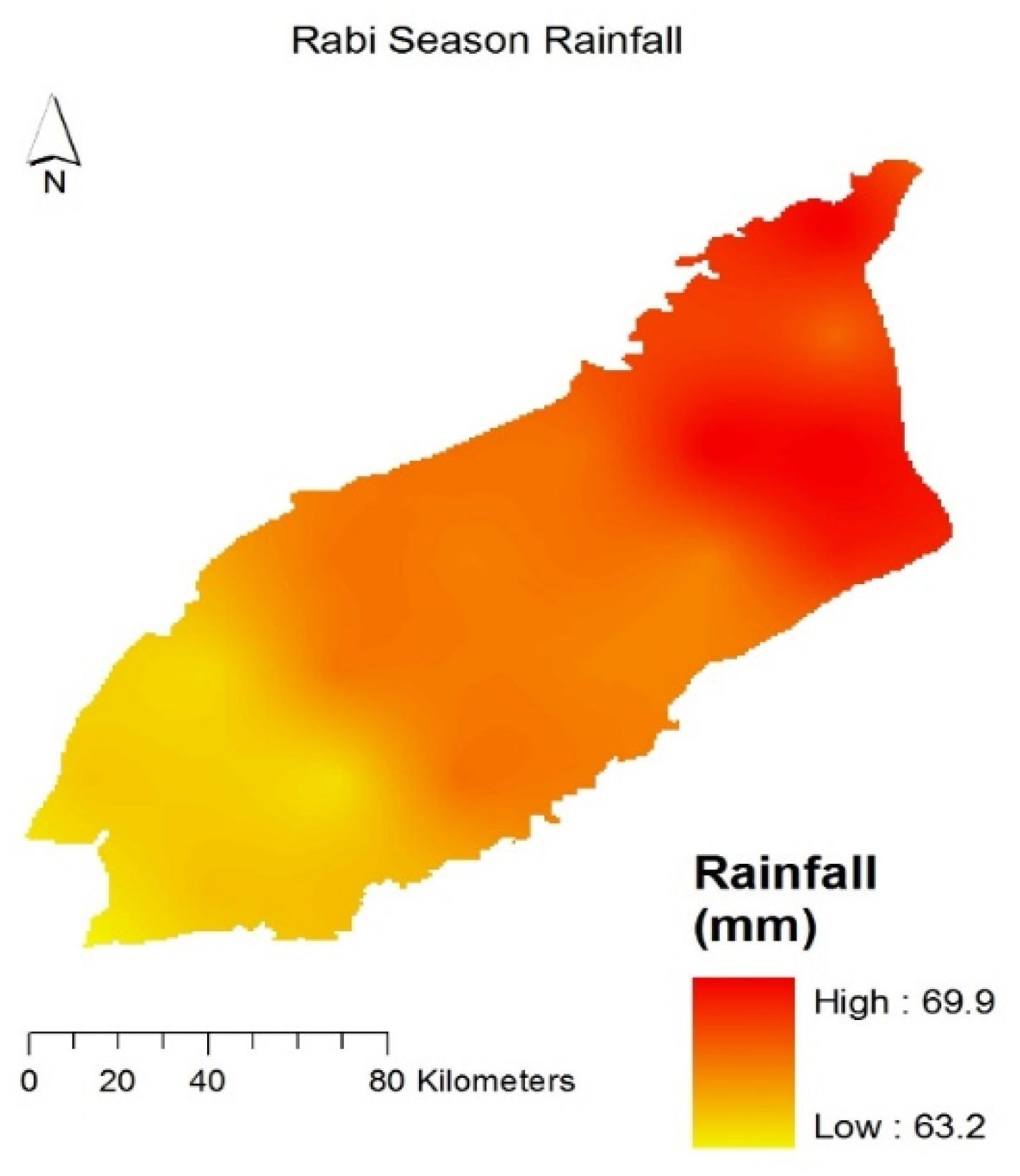
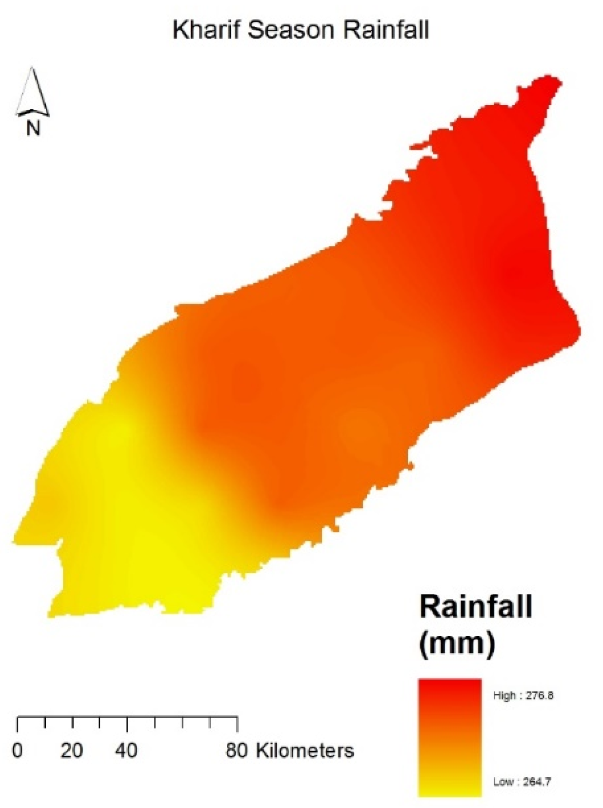
The geo-informatics approach provides enough efficiency for the application of the water balance approach in the unsaturated zone for the quantification of groundwater components [14,16]. Surface water supplies are usually considered as the equally distributed depth of water throughout the canal command area [14,16,18,19]. In the case of a reliably dense meteorological station, spatial distribution of rainfall is assessed through interpolation [19], while, in data scare basins, Tropical Rainfall Measuring Mission (TRMM) is mostly adopted for assessments of the spatial distribution of rainfall [20]. Further, calibration and validation of the TRMM with the point sources data increase its reliability in the water balance studies [20,21].

Remote sensing and GIS applications are widely used for the spatio-temporal mapping of the water resources management components. Ref. [22] evaluated the water management components using the SEBS algorithms at the Indus Basin Irrigation System. Ref. [21] estimated the consumptive water use using the surface energy balance algorithm in the LCC system. Ref. [23] estimated the irrigation system performance and assessed the consumptive water use using the soil energy balance algorithm for land in the Rechna Doab. Ref. [24] assessed the equity of canal water and groundwater at the canal command area of Hakara system using remote sensing and a GIS-based approach. Ref. [25] assessed the canal water deficit using remote sensing and a GIS-based approach. Ref. [26] applied remote sensing and hydrological modeling for the irrigation system performance. Ref. [27] used remote sensing for mapping and assessment of water use in central Asia.

The research objective of the current study was the estimation of the critical water management components in the largest irrigation scheme of the Indus basin for the period of (2011–2012 to 2014–2015). The distribution and the availability of the water resources management components at fine spatial and temporal resolution can help policymakers to develop effective water management strategies to enhance water productivity.

2. Methodology

2.1. Study Area

The lower Chenab canal system is the oldest and the largest irrigation system in the Indus Basin Irrigation System. The canal command area is between the two rivers (Ravi and Chenab) of Pakistan (Figure 1). The area of the LCC system is about 1.24 million ha (Mha). The climate of the study area is considered semiarid with an average annual rainfall of 380 to 400 mm. The cropping pattern of the irrigation system is wheat as the major winter crop and rice, cotton, and maize as the major Kharif crop. Crop water requirement is fulfilled from surface and groundwater resources. The network of the irrigation system has seven main distributaries. Water from these distributaries is further diverted to the sub-channels to deliver water in the farmer’s field channels. Water distribution is fixed based on the water allowance from the irrigation department for each hierarchy of channels. Participatory management-based decisions, cost recovery, and distribution uniformity are core responsibilities of the Farmers Organization (FOs). FOs members are farmers from the representative distributary of the irrigation system. Further, these FOs elected the chairman of the water board of the whole irrigation system, i.e., LCC.

Canal water is the main source of irrigation in the LCC system along with a significant proportion of groundwater. The lower Chenab canal system is distributed into seven main distributaries. All these distributaries are monitored by the Program Monitoring and Implementation Unit (PMIU) of the Punjab Irrigation Department. Irrigation efficiency is a product of field and irrigation network efficiency. Irrigation efficiency was incorporated from the study of [6] that defines the field efficiency of 75% and the irrigation network efficiency of 48%. According to the aforementioned definition of irrigation efficiency, 36% irrigation efficiency of the system was obtained.

2.2. SEBAL for the Estimation of Actual Evapotranspiration

Surface Energy Balance Algorithm for Land (SEBAL) is widely used for the estimation of the actual evapotranspiration in hydrological studies. The input used in this energy balance was the satellite-derived remote sensing imagery. SEBAL was successfully used in the water balance studies at different temporal and spatial scales [16,21,28,29,30] researched in Pakistan and provided the theory of the SEBAL algorithm. The methodology was successfully applied in the IBIS by [31]. The residual of the energy budget was actual evapotranspiration, which is demonstrated below (Equation (1)).

$$R_n=G_o+H+\lambda E$$

(1)

where, R_n, G_o, H, and λE represent net radiation (W m⁻²), soil heat flux (W m⁻²), sensible heat flux (W m⁻²), and latent heat flux (W m⁻²), respectively.

The concept of evaporative fraction was introduced by [16] and, based on this concept, latent heat flux can be represented (Equation (2)) by considering net available energy (R_n − G_o) and evaporative fraction:

$$\lambda E=\mathsf{\Delta }\left(R_n-G_o\right)$$

(2)

where, Δ = evaporative fraction and was formulated as:

$$\mathsf{\Delta }=\frac{\lambda E}{R_n-G_o}=\frac{\lambda E}{\lambda E+H}$$

(3)

Net available energy can be calculated from instant, daily, or monthly timescales. For the calculation of the daily ET, soil heat flux can be ignored at the time scale of one day, and net radiation (R_n) is considered as the net available energy. Daily ET can be calculated as Equation (4):

$$E{T}_{24}=\frac{86400\times {10}^3}{\lambda \times {\rho }_w}\times \mathsf{\Delta }\times R_{n24}$$

(4)

where, R_n24, λ, and ρ_w describe the 24 h averaged net radiation, latent heat of vaporization, and water density, respectively.

Ref. [32] described the important variables for ET estimation, including land cover, land surface albedo, and land surface temperature. Remote sensing estimated the variables possible using different satellite sensors [30]. MODIS product was used due to its superior spatiotemporal resolution and spectral bands. The MODIS standard products can be downloaded for free from the USGS website https://lpdaac.usgs.gov/get_data/data_pool (accessed on 3 March 2021).

Table 1. MODIS products used in this study.

Product Name	Dataset Used	Spatial Resolution (m)	Sensor
MOD09Q1	Land surface reflectance (band 1 and band 2)	250	TERRA
MOD11A2	Land surface temperature and emissivity	1000	TERRA
MOD13A2	NDVI	1000	TERRA

describes the detail of the product used in this study.

2.3. Advection Aridity Approach

The advection aridity (AA) model was successfully used by many researchers under different climatic conditions. With the water balance and the eddy covariance methods [33,34,35] applied, the advection aridity method at the basin scale showed good agreement with SEBS. Ref. [36] applied the AA model at a regional scale and found good agreement between SEBAL and AA models. Ref. [34] applied three different methods for mapping the ETa in China and found the AA model most accurate. Firstly, [37] proposed the AA model using [38] for the wet surface ET as formulated in Equation (5). For the potential evapotranspiration, [39]’s equation was used as given below (Equation (6)), and an empirical wind function was used, as given below in Equation (7).

$$E{T}_w={\propto }_e\frac{\mathsf{\Delta }}{\mathsf{\Delta }+\gamma }\left(R_n-G\right)$$

(5)

$$E{T}_p=\frac{\mathsf{\Delta }}{\mathsf{\Delta }+\gamma }\left(R_n-G\right)+\frac{\gamma }{\mathsf{\Delta }+\gamma }\times E_r$$

(6)

$$E_r=f\left(U_2\right)\times \left(e_s-e_a\right)$$

(7)

$$f\left(U_2\right)=0.26\left(1+0.54U_2\right)$$

(8)

where, ${\propto }_e=1.26$ is the Priestly and Taylor coefficient, and variables $\left(R_n-G\right)$,$\mathsf{\Delta }$, $\gamma$, $U_2$, $e_s$ and $e_a$ represents the available energy at the surface, slope of saturated water vapor pressure curve at the current time (kP °C⁻¹), psychometric constant (kP °C⁻¹), mean wind speed above the 2 m of the ground surface, saturated vapor pressure and actual vapor pressure respectively. Ref. [37] combined the potential ET (Equation (5)) and the wet surface ET (Equation (6)) following the relationship given by [40], as shown below (Equation (9)):

$$AET=\left(2{\propto }_e-1\right)\frac{\mathsf{\Delta }}{\mathsf{\Delta }+\gamma }\left(R_n-G\right)-\frac{\mathsf{\Delta }}{\mathsf{\Delta }+\gamma }\times 0.26\left(1+0.54U_2\right)\left(e_s-e_a\right)$$

(9)

In this study, due to the unavailability of the directly measured ET, the AA model was used for the evaluation of SEBAL estimated ETa. The climatic data used for the AA model were collected from the University of Agriculture, Faisalabad, and the Pakistan Meteorological Department.

2.4. Satellite Derived Rainfall

The Pakistan Meteorological Department (PMD) is responsible for the measurement of meteorological data at a regional scale. There are 97 total observatories in Pakistan (PMD online source). However, there are only two observatory stations in the study area. GIS-based interpolation was not found appropriate for the low-resolution dataset. Therefore, satellite-based raster data were acquired with a spatial resolution of 25 km along with monthly temporal resolution using Tropical Rainfall Measurement Mission (TRMM). Low-resolution rain gauge availability creates a limitation for the calibration of TRMM data. Ref. [41] provided the solution under this limited environment by averaging the measurement over time. Therefore, 3B43 product was accumulated into seasonal basis using the cropping pattern. The Kharif season includes mid-April to the middle of November. Following the experience of [36], local calibration and validation of this data were performed with point observatory data. Monthly rainfall data were summed up to obtain seasonal rainfall for all Kharif and Rabi seasons. Further, GIS was used to extract the data from each pixel, and the detailed data were interpolated using kriging to create the high-resolution map.

2.5. Groundwater Irrigation

Net groundwater irrigation at the spatial scale of distributaries and two temporal scales of LCC were estimated using geo-informatics techniques. This approach provides the advances above conservative and indirect approaches [22]. Satellite-derived actual evapotranspiration was used as a key component for the establishment of a water balance approach in the unsaturated zone. This approach was successfully applied by [16] (Equation (10)).

$$NGWI=E{T}_a-P_e-NCWI$$

(10)

where, NCWI, P_e, and NGWi describe net canal water irrigation, effective rainfall, and net groundwater irrigation, respectively.

This approach provided the net groundwater irrigation that was the water used by the plants or evaporated from the area under consideration, while the pumping from the aquifer was more than the net groundwater irrigation due to the inefficient delivery system of irrigation. Therefore, groundwater abstraction was estimated using the field application efficiency. In this study, the results of [6] were used that showed field application efficiency of 75% and network efficiency of 90%. This resulted in 68% irrigation efficiency of the system. The framework of the study is shown in Figure 2.

3. Results

3.1. Canal Water Availability

Regarding estimation of canal water availability, the maximum gross canal water (GCW) irrigation depth of 343 mm was found during the 2014–2015 cropping year, while in the cropping year of 2011–2012, the GCW was found at a minimum with the value of 305 mm for the LCC (

Table 2. Gross canal water distribution (mm) in LCC from 2011–2012 to 2014–2015.

Annual	Rabi Season							Kharif Season
	Nov.	Dec.	Jun.	Feb.	Mar.	1–15 Apr.	Total Rabi	16–30 Apr.	May	Jun.	Jul.	Aug.	Sept.	Oct.	Total Kharif	Total Annual
2011–2012	27.3	26.2	13.7	0	24.4	11.4	103.1	11.5	19.1	26.9	39.6	40.1	35.4	29.2	201.9	305.8
2012–2013	23.8	25.0	12.5	8.5	28.9	14.7	113.5	14.3	31.8	36.7	39.6	40.2	35.5	29.3	227.3	340.8
2013–2014	29.50	26.25	12.47	15.27	25.87	13.21	122.57	13.26	30.83	37.20	40.02	41.04	17.06	34.82	214.23	336.8
2014–2015	29.57	29.44	9.10	8.15	21.09	12.99	110.34	15.37	36.11	33.15	39.41	40.93	37.32	30.67	232.96	343.3
Average	27.55	26.73	11.94	7.96	25.08	13.10	112.38	13.59	29.46	33.50	39.67	40.56	31.32	30.99	219.12	331.7

). Water supply during Kharif season was 32% more than Rabi season due to canal closure during Rabi. Every year, for the removal of accumulated silt in the irrigation system, canals remain closed during December and January [42] and sometimes for the month of February. During the spatial analysis, the gross canal water distribution was found to be maximum at the Upper Gugera, while the minimum was the Sagar distributaries (Figure 3). The distribution of gross canal water from the LCC system was minimal during the month of February and maximal during the months of July and August. This lower canal water availability in the month of February was due to the closure of the canal for the annual removal of silts from the irrigation system. The maximal levels in July and August were due to the maximum surface water availability in the Indus basin due to heavy snow melting and monsoon rainfall. Net canal water distribution (mm) in LCC from 2011–2012 to 2014–2015 is shown in

Table 3. Net canal water distribution (mm) in LCC from 2011–2012 to 2014–2015.

Annual	Rabi Season							Kharif Season
	Nov.	Dec.	Jun.	Feb.	Mar.	1–15 Apr.	Total Rabi	16–30 Apr.	May	Jun.	Jul.	Aug.	Sept.	Oct.	Total Kharif	Total Annual
2011–2012	9.8	9.4	4.9	0.0	8.8	4.1	37.1	4.1	6.9	9.7	14.3	14.4	12.8	10.5	72.7	110.1
2012–2013	8.6	9.0	4.5	3.0	10.4	5.3	40.9	5.1	11.4	13.2	14.3	14.5	12.8	10.5	81.8	122.7
2013–2014	10.6	9.5	4.5	5.5	9.3	4.7	44.1	4.7	11.1	13.3	14.4	14.7	6.1	12.5	77.1	110.1
2014–2015	10.6	10.5	3.2	2.9	7.5	4.6	39.7	5.5	12.9	11.9	14.1	14.7	13.4	11.0	83.8	123.5
Average	9.9	9.6	4.3	2.9	9.0	4.7	40.5	4.9	10.6	12.1	14.3	14.6	11.3	11.2	78.9	119.4

.

3.2. Calibration and Validation of SEBAL with Advection Aridity Method

None of the previous researchers deny the validation of the SEBAL model. Validation was done with the available data source of ET measurements such as Bowen ration energy balance [43], meteorological data [44], advection aridity method [36], and eddy covariance [45]. Ref. [34] found the AA to be the most accurate method after applying three different techniques for mapping the ETa at a regional scale in China. Validation of SEBAL is important for further use in hydrological studies. The calibration process was carried out by using SEBAL pixels and meteorological data available at the nearby climate monitoring station and is shown in Figure 4. SEBAL was successfully validated with the AA model by [36] at the regional scale studies in the Indus Basin Irrigation System. The results obtained were satisfactory for Rabi and Kharif seasons. Nash suit cliff efficiency was found to be higher in Rabi season as compared to Kharif season. Similarly, low bias values were found in the Rabi season relative to the Kharif season. The results are supported by the outcomes of [21]. Similarly, [34,46] argued that AA models work well during cold seasons. A significant difference in the ET was found for both seasons. Ref. [36] argued that this difference was due to the difference in climatic condition, change in crop type, and water availability. The variation in the ET was found from the upper reaches to the lower reaches of the LCC system with the same crop type. For the Kharif season, the difference was higher than the Rabi season. This variation was 9.63 mm for the rice crop, 9.71 mm for cotton, and 10.2 mm for sugarcane. For the Rabi crop, wheat variation was 1.03%, and sugarcane variation was 1.05%. Usman et al. (2014) argued that this variation increases if the analysis is performed at a finer resolution. Figure 4 represents the calibration and the validation of SEBAL with AA. Statistical analysis of seasonal and annual ETa (mm) of SEBAL and AA are explained in

Table 4. Statistical analysis of seasonal and annual ETa (mm) of SEBAL and AA.

Season	Mean		Standard Deviation		Goodness of Fitness of Measure
	SEBAL ETa	AA ETa	SEBAL ETa	AA ETa	R	NSE	PBIASE	RMSE
Kharif	87.1	100.0	27.7	34.9	0.93	0.72	−12.9	34.9
Rabi	47.9	55.3	15.9	16.1	0.94	0.85	−4.4	5.76
Annual	69.0	77.0	30.1	42.4	0.97	0.83	10.4	17.0

.

3.3. Spatially Distributed ETa

Seasonal analysis of Eta revealed 47% more ETa during the Kharif season as compared to the Rabi season, while the variation in the annual scale analysis showed less variation (

Table 5. Actual evapotranspiration distribution (mm) in LCC from 2011–2012 to 2014–2015.

Annual	Rabi Season							Kharif Season
	Nov.	Dec.	Jun.	Feb.	Mar.	1–15 Apr.	Total Rabi	16–30 Apr.	May	Jun.	Jul.	Aug.	Sept.	Oct.	Total Kharif	Total Annual
2011–2012	41.2	34.4	28.2	41.6	71.4	41.4	258.2	38.3	108.8	106.6	104.3	108.4	84.3	61.2	611.9	870
2012–2013	32.8	38.2	32.2	51.0	85.1	46.3	285.6	38.7	101.4	109.4	107.5	111.6	83.4	51.5	603.5	889
2013–2014	40.4	41.2	42.4	58.4	81.2	49.6	313.2	35.1	107.6	105.4	108.6	112.4	86.7	59.2	615	928
2014–2015	42.6	36.2	42.5	38.4	83.4	46.2	289.3	36.6	104.5	108.4	121.2	110.1	84.6	54.4	619.8	902
Average	39.2	37.5	36.3	47.3	80.3	45.8	286.5	37.2	105.5	107.5	110.4	110.6	84.7	56.5	612.5	899

). High ETa during Kharif was due to more surface water availability in the irrigation system along with the growing period of the high water demanding crops such as cotton and rice as compared to wheat. The month-based analysis revealed the variation in ETa with the minimum average value of 23 mm in January and a maximum average value of 123 mm in August and a four year average annual value of 897 mm during the study period (2010–2011 to 2014–2015). In the case of temporal analysis, May to August showed the peak rates of ETa, while, in the case of spatial analysis, peak rates were observed in rice-cropped areas. Similarly, December to January showed the lowest ETa rates due to less water supply along with decreased crop water requirements [42]. During the design of the LCC irrigation system, the cropping intensity was considered 75% [47]. Though, it increased more than double its design due to the green revolution of the 1960s. Despite this significant increase in demand due to high cropping intensity, the deliveries from the canal water remain stagnant, which causes a big gap between canal water availability and its demand and leads towards the severe scarcity in the region.

Figure 5 and Figure 6 show the four years average of Rabi and Kharif season ETas, respectively, at the LCC system. The ETa map shows the significant variation in the actual evapotranspiration; the actual evapotranspiration was high at the head reaches of the LCC system. This higher ETa was due to more rice cultivation at the head reaches than the tail of the irrigation system, while, in the Rabi season, ETa was found higher from the center to the lower part of the system. This higher ET was due to the cultivation of more Rabi fodder crops than Kharif crops, especially the cultivation of the berseem crop.

Figure 7 shows the distribution of ETa in different canal command areas (CCAs) during the last four years (2010–2011 to 2014–2015). There was no significant temporal variation in the ETa between different CAs. In the case of Sagar CCA, the average ETa was 903 mm with a standard deviation of 12.5 mm. Mian Ali canal command showed the maximum standard deviation of 20 mm and Jhang canal command showed the lowest standard deviation of 12 mm. Due to fixed water allowance, stagnant resources, and locally fixed cropping zone, there were no changes in supply of irrigation water, practices of irrigation method, and or cropping patterns. Rakh and Mian Ali canal command showed low average ETa values as compared to the CCAs in the system. Likewise, Mian Ali and Rakh canal command areas had poor quality groundwater. Maximum ET at the Sagar canal commands was due to its location upstream of the irrigation system and cultivation of rice crop.

3.4. Spatially Distributed Rainfall

The existing studies describe over- and underestimations of rainfall from the TRMM relative to the changes in topography. Ref. [20] described, in detail, over- and underestimations of rainfall from the TRMM in the Indus basin. Similarly, [48] described the similar trend of rainfall over- and underestimations in Bangladesh. Further, [49] described that that satellite overestimated the rainfall in areas with the rainfall <400 mm month⁻¹ and underestimated in the areas of rainfall >400 mm month⁻¹. These results were further strengthened by the findings of [48]. They concluded that the TRMM has limitations in accurate rainfall detection at low or high rainfall rates. Thus, in the study area, TRMM overestimated the rainfall that was calibrated with the point observatory data. The spatial distributions of rainfall for Rabi and Kharif seasons are shown in Figure 8 and Figure 9, respectively. These figures clearly show the decrease in rainfall towards the tail of the irrigation system.

Table 6. Rainfall distribution (mm) in LCC from 2011–2012 to 2014–2015.

Annual	Rabi Season							Kharif Season
	Nov.	Dec.	Jun.	Feb.	Mar.	1–15 Apr.	Total Rabi	16–30 Apr.	May	Jun.	Jul.	Aug.	Sept.	Oct.	Total Kharif	Total Annual
2011–2012	0	0	3.8	8	1.5	7.5	20.8	2.7	0	23.6	45.4	38.5	163.7	11.5	285.4	306.2
2012–2013	0	17.2	1.5	55	1.3	12.7	87.7	8.9	4.6	67.5	4.7	114.9	3.3	0	203	290.7
2013–2014	0.5	0	0	14.3	41.7	10.3	66.8	18	41.2	7.1	57.5	4.8	140.2	3.6	272.4	339.2
2014–2015	10	0	12.2	20.5	67.9	32.8	143.4	0	17	11.6	128	48.4	75.2	14.5	294.7	438.1
Average	2.63	4.3	4.38	24.5	28.1	15.8	79.7	7.4	15.7	27.5	58.9	51.7	95.6	7.4	264.2	343.5

and

Table 7. Effective rainfall distribution (mm) in LCC from 2011–2012 to 2014–2015.

Annual	Rabi Season							Kharif Season
	Nov.	Dec.	Jun.	Feb.	Mar.	1–15 Apr.	Total Rabi	16–30 Apr.	May	Jun.	Jul.	Aug.	Sept.	Oct.	Total Kharif	Total Annual
2011–2012	0	0	3.1	6.4	1.2	6	16.7	2.2	0	18.9	36.3	30.8	130.9	9.2	228.3	244.9
2012–2013	0	13.8	1.2	44	1.04	10.5	70.2	7.1	3.7	54	3.8	91.9	2.6	0	163.1	232.6
2013–2014	0.4	0	0	11.4	33.4	8.2	53.4	14.4	33	5.7	46	3.8	112.6	2.9	217.9	271.4
2014–2015	8	0	9.8	16.4	54.3	26.2	114.7	0	13.6	9.3	102.4	38.7	60.2	11.6	235.8	350.5
Average	2.1	3.5	3.5	19.6	22.5	12.7	63.9	5.9	12.6	21.9	47.2	41.3	76.6	5.9	211.4	274.8

describe the temporal analysis of gross and effective rainfalls. Table 6 shows the temporal rainfall distribution. The maximum mean monthly of four years of rainfall was found at a maximum of 95.6 mm in September and a minimum of 2.6 mm in November. The average annual rainfall for the four years was 343.5 mm.

Rainfall results are shown in Table 7. The annual effective rainfall variation ranged between 232.6 mm year⁻¹ and 350.8 mm year⁻¹, with an average of 274 mm year⁻¹ during 2010–2011 to 2014–2015. Variation in the mean monthly analysis for effective rainfall showed variations of 2.1 mm (minimum) in November and 76.5 mm (maximum) in September. The rainfall that occurred during the months of monsoon (June–September) was more than 55 mm month⁻¹. The analysis of seasonal rainfall occurrence found averages of 23% during Rabi and 77% during Kharif for total rainfall amount.

Figure 10 shows the effective rainfall in different CCAs during the last four years (2011–2012 to 2014–2015). The maximum four years average annual effective rainfall in the LCC irrigation scheme was 302 mm at the Sagar. Figure 10 shows that there were significant temporal variations in the effective rainfall at each CCA, while there was no significant average annual rainfall between different CCAs, as shown in the figure. The maximum average four years effective rainfall was 302 mm at Sagar, and the minimum was 258 mm at the Burala branch.

3.5. Groundwater Irrigation

In arid and semi-arid areas, groundwater is a complementary source of irrigation under high cropping intensity. Groundwater contribution is significant in the IBIS. Ref. [16] described 42% of the groundwater pumping at the head of the irrigation system. Groundwater irrigation results showed that groundwater has a significant share to fulfill the irrigation water demand. The groundwater irrigation map obtained from the water balance described the significant groundwater contribution at the head of the canal system. Irrigation water supply from the system was aggregated to monthly, seasonal, and annual irrigation water volumes. Based on spatial mapping, four years’ average net groundwater irrigation range was found from 195 mm to 88 mm during Rabi season and 314 mm to 99 mm during the Kharif season. The four years average of gross groundwater abstraction (GWA) was a maximum of 750 mm at the upstream areas of the irrigation system. The minimum GWA was 275 mm at the tail of the LCC system. This described more use of canal water at the head of the irrigation system. Four years average share of the net groundwater irrigation (NGWI) was 283 mm, which represented 44% of the average annual supply of canal water (Figure 11 and Figure 12). The contribution of the average annual groundwater in the ETa was 42%. The monthly maximum average NGWI was during the month of May, whereas the minimum was during the month of November.

The remaining crop water requirement is highly dependent on groundwater use, as the sum of the rainfall plus the irrigation water supply is less than the demand. The sum of both surface water sources (net canal plus rainfall) four years average in the study period was found to be 548 mm (36% of ETa). Therefore, farmers depend on the use of groundwater to fulfill the irrigation water need. The average of the study period showed 739.6 mm of groundwater abstraction, while the annually based variation ranged between 632 mm and 780 mm. Seasonal analysis revealed 39% and 61% of groundwater abstraction proportions during Rabi and Kharif seasons, respectively (

Table 8. Distribution of net groundwater irrigation (mm) in LCC from 2011–2012 to 2014–2015.

Annual	Rabi Season							Kharif Season
	Nov.	Dec.	Jun.	Feb.	Mar.	1–15 Apr.	Total Rabi	16–30 Apr.	May	Jun.	Jul.	Aug.	Sept.	Oct.	Total Kharif	Total Annual
2011–2012	31.2	24.6	20.0	47.6	61.0	30.9	215.2	31.7	101.1	77.4	53.4	62.8	0	41.3	308.0	523.0
2012–2013	23.4	15.2	26.3	4.0	73.5	30.5	173.0	25.7	85.9	41.8	89.0	4.6	67.6	40.5	355.8	528.7
2013–2014	29.0	31.6	37.5	41.1	38.3	36.0	213.4	15.8	62.9	85.9	47.6	93.4	0	43.6	31.7.0	530.4
2014–2015	23.4	25.4	29.0	18.7	21.1	15.1	132.6	30.5	77.4	86.8	4.4	56.5	10.4	31.4	297.4	297.9
Average	26.7	24.2	28.2	27.8	48.5	28.1	183.6	25.9	81.8	73.0	48.6	54.3	19.5	39.2	319.5	503.0

). The fluctuations in four cropping years for monthly groundwater abstraction ranged between 28.7 mm and 120.3 mm. This variation was high in the 2011–2012 to 2012–2013 cropping year (0 mm to 148.7 mm); this variation is dependent upon the occurrence of rainfall and crop phenology. This lowest abstraction in September could be due to high monsoon rainfall and to less water demand. Net groundwater irrigation estimated after incorporating the efficiencies was 503 mm year⁻¹ (

Table 9. Distribution of gross groundwater abstraction (mm) in LCC from 2011–2012 to 2014–2015.

Annual	Rabi Season							Kharif Season
	Nov.	Dec.	Jun.	Feb.	Mar.	1–15 Apr.	Total Rabi	16–30 Apr.	May	Jun.	Jul.	Aug.	Sept.	Oct.	Total Kharif	Total Annual
2011–2012	45.8	36.1	29.4	70.0	89.7	45.4	316.5	46.6	148.7	113.9	78.6	92.3	0	60.7	452.9	769.0
2012–2013	34.4	22.4	38.7	5.8	108.1	44.9	254.4	37.9	126.3	61.4	130.8	6.8	99.4	59.5	523.2	777.6
2013–2014	42.6	46.4	55.2	60.4	56.4	52.9	313.9	23.3	92.6	126.4	70.0	137.3	0	64.1	466.1	780.0
2014–2015	34.3	37.4	42.6	27.5	31.0	22.2	194.9	44.8	133.8	127.6	6.5	83.2	15.3	46.1	437.3	632.3
Average	39.3	35.6	41.5	40.9	71.3	41.4	269.9	38.1	120.3	107.3	71.5	79.9	28.7	57.6	469.9	739.7

) on average for the four cropping years. Unlike surface water use from canals, the maximum groundwater use in the month of May was due to the cultivation of rice as well as insufficient rainfall and canal water availability.

Figure 13 shows the gross groundwater irrigation (GGWA) in LCC system CCAs during the last four years (2010–2011 to 2014–2015). The four years average annual GGWA was found to be 526 mm for the whole LCC system. There was significant temporal variation in GGWA in the CCAs of the LCC system (Figure 13). The four years average gross groundwater abstraction was 887 mm at the Sagar, and the minimum was at the Upper Gugera with zero groundwater abstraction for this study period. This was due to the maximum canal water supply to the Upper Gugera. The maximum abstraction was in the Sagar CCA, while the minimum abstraction was in the Upper Gugera CCA. Higher GGWA in the Sagar CCAS was due to the intensive cultivation of rice crop.

4. Discussion

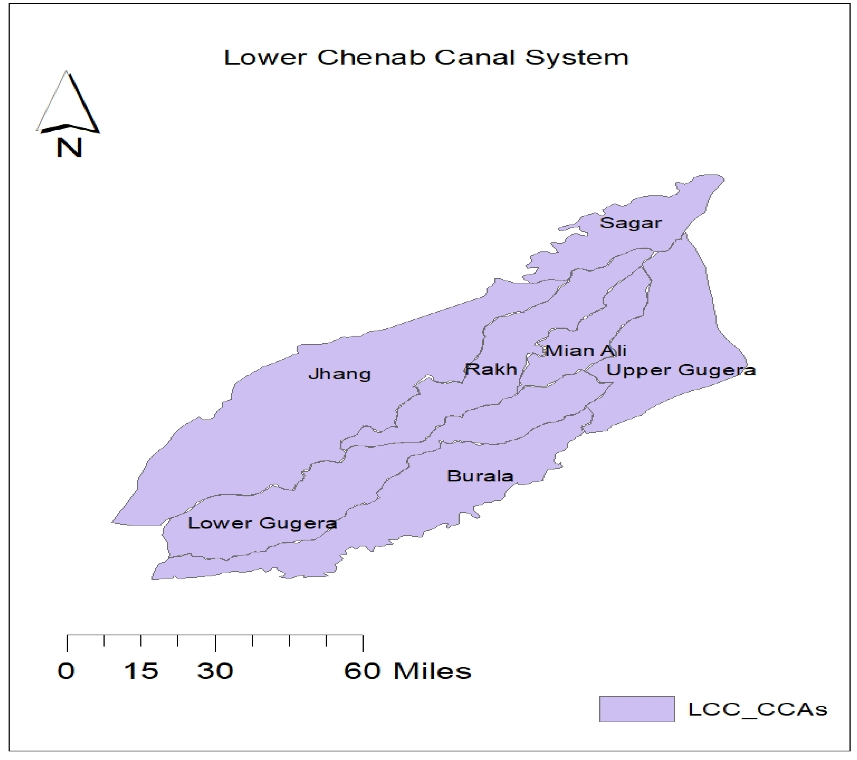
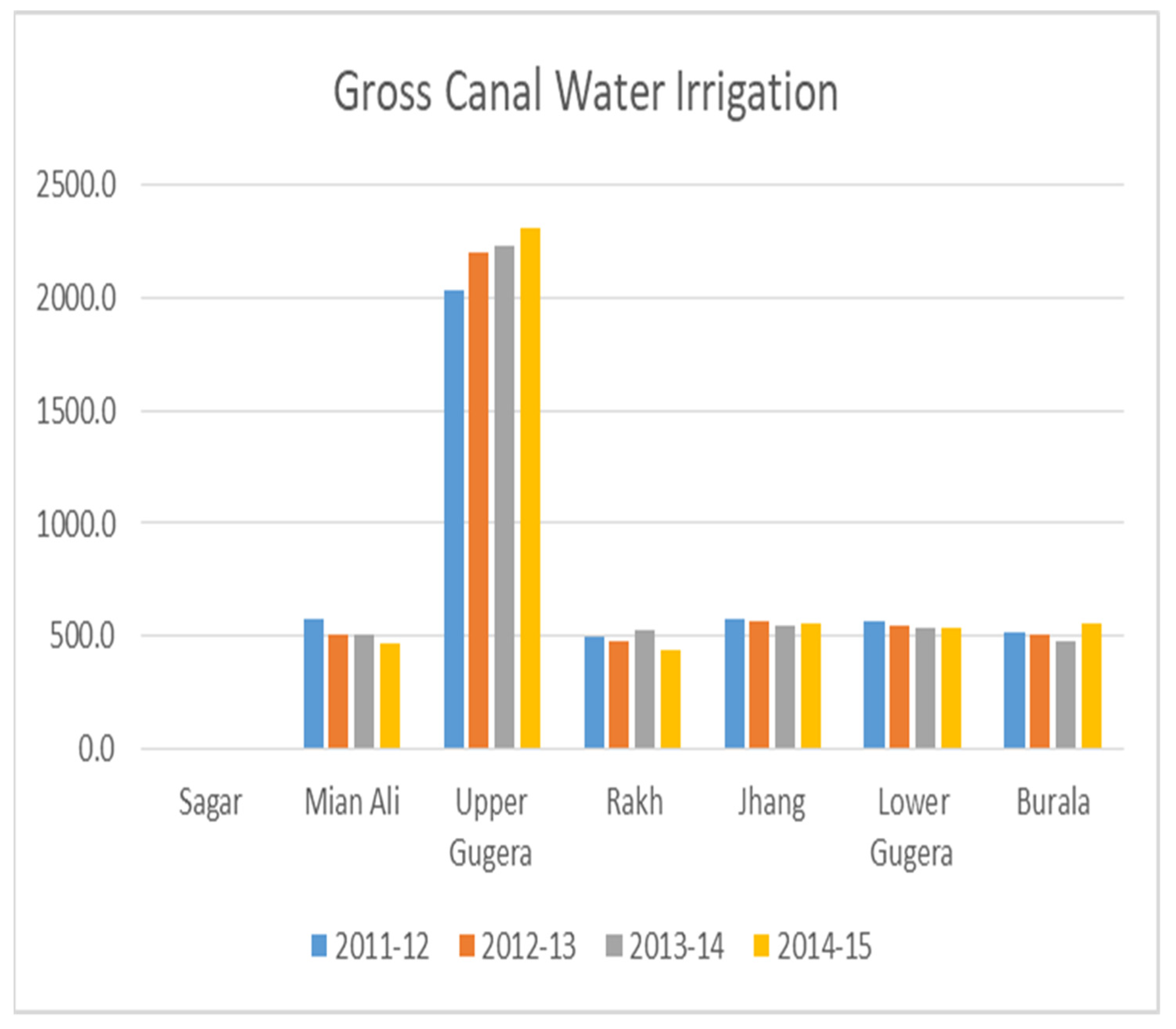
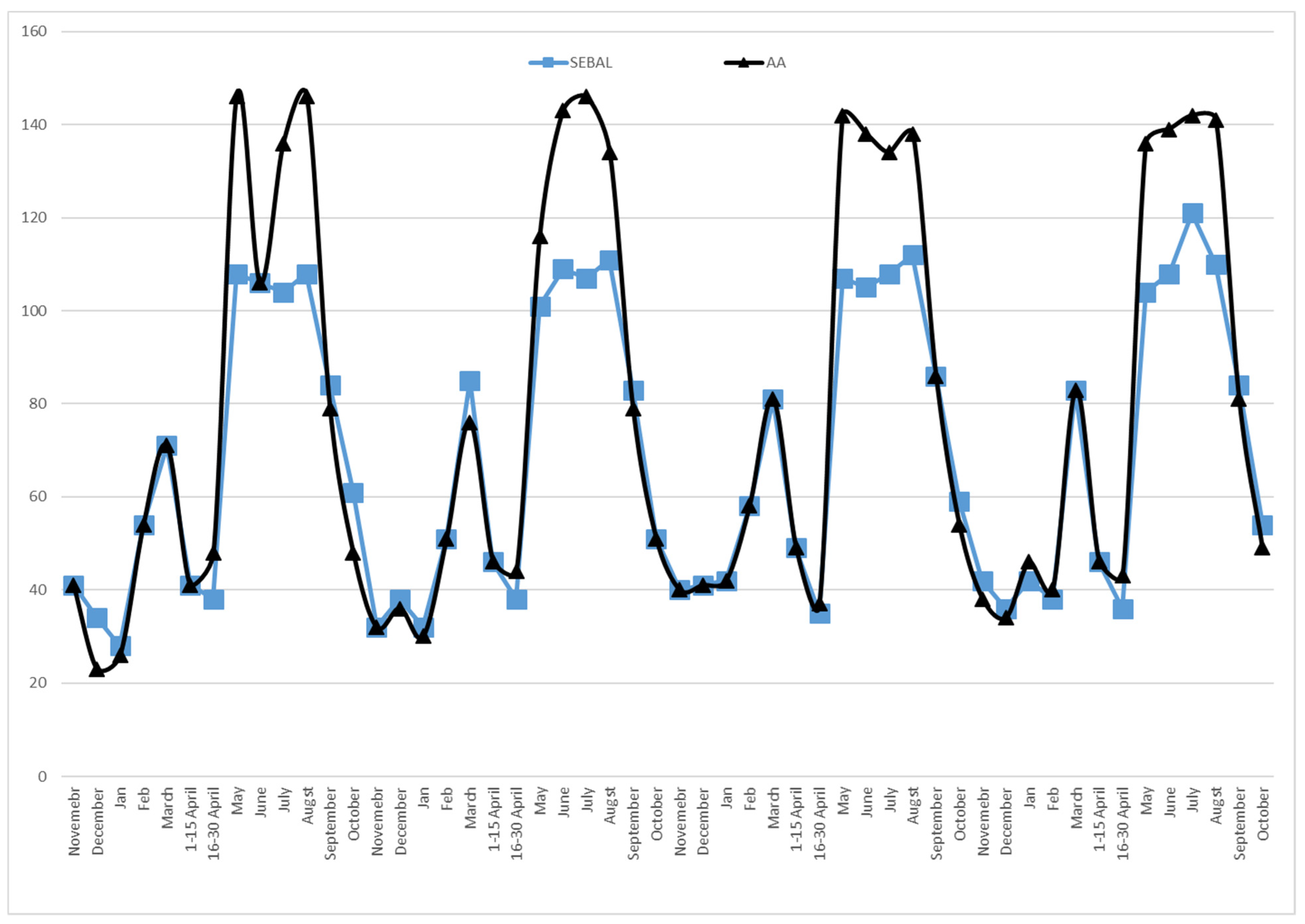
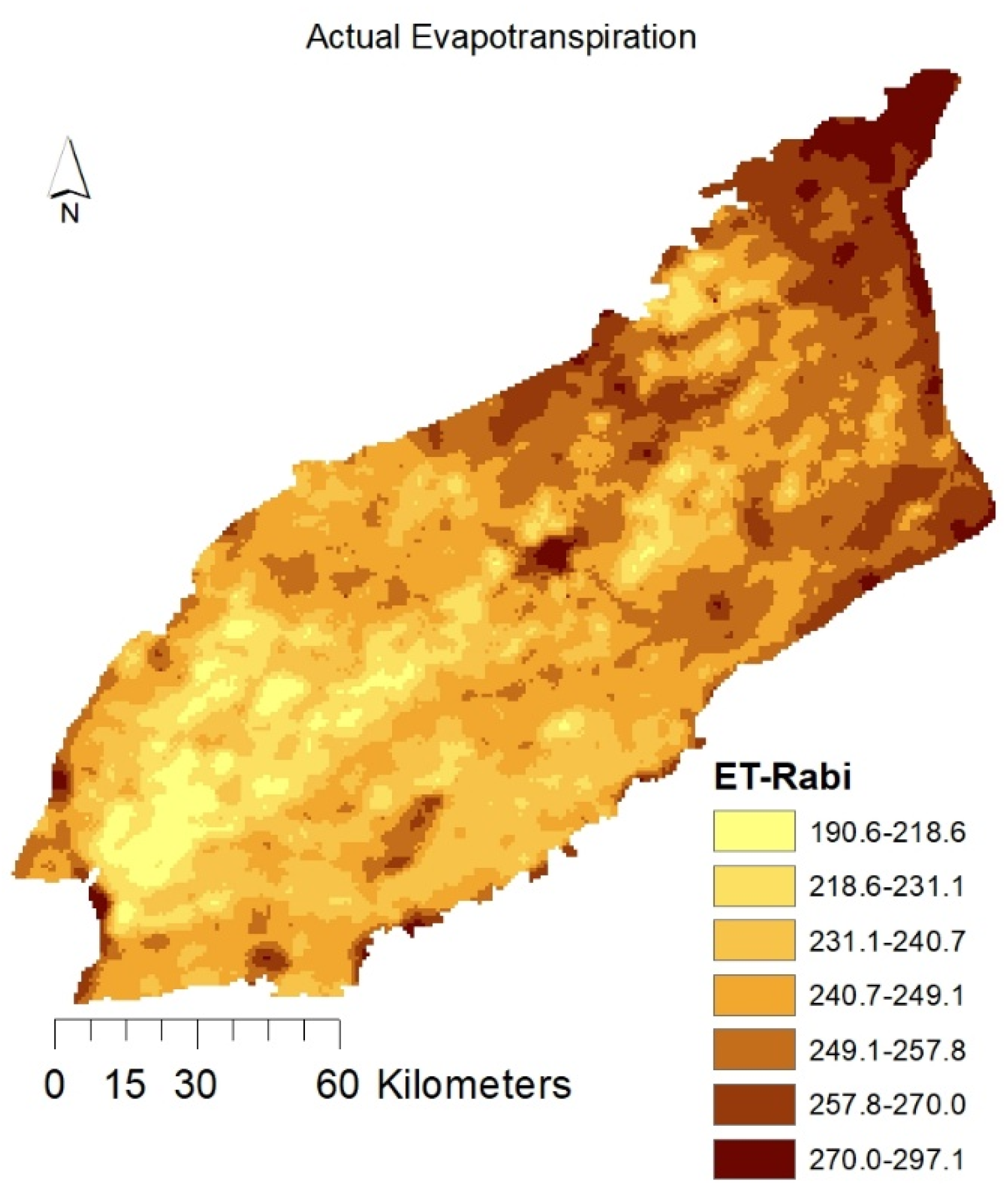
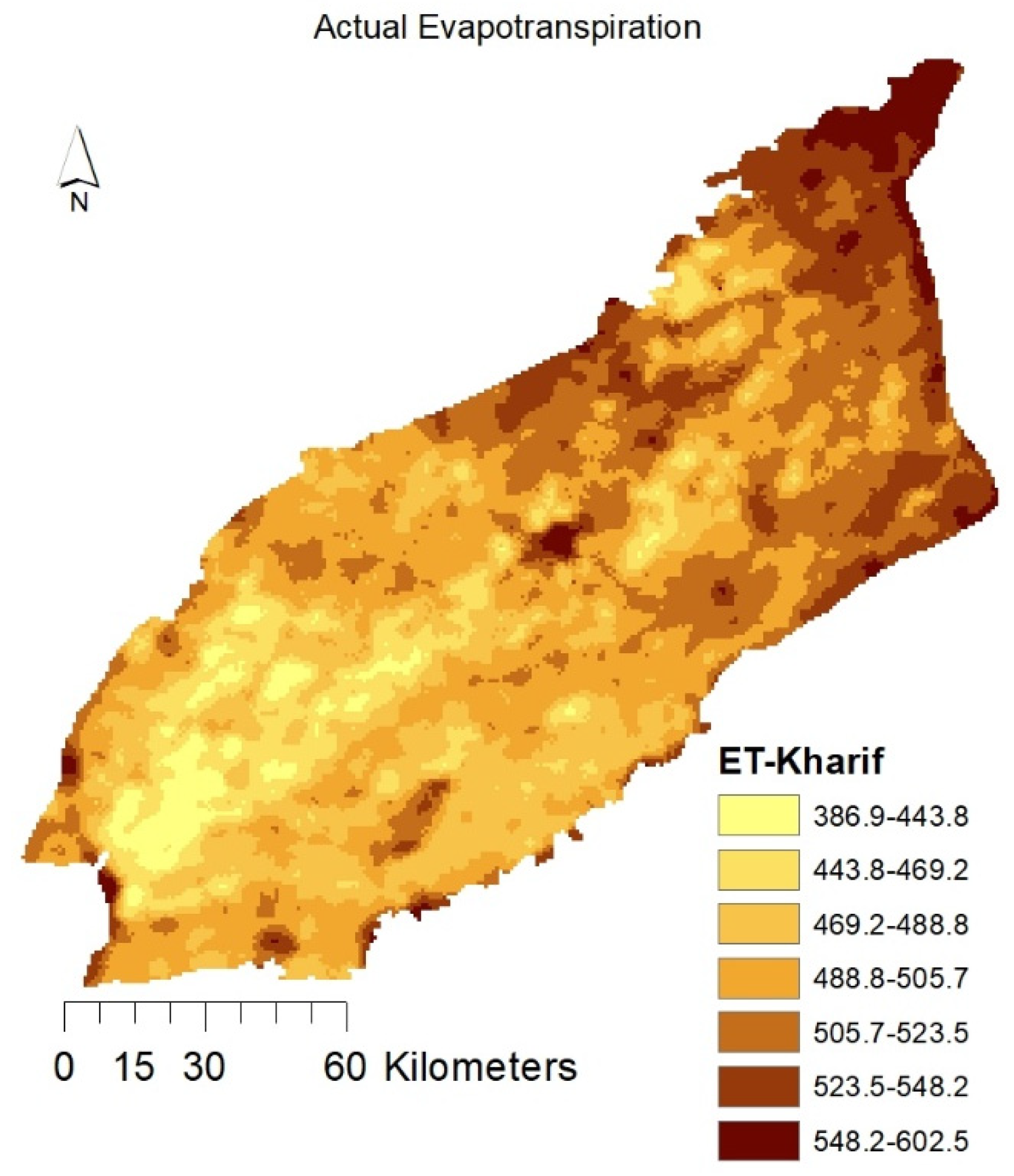
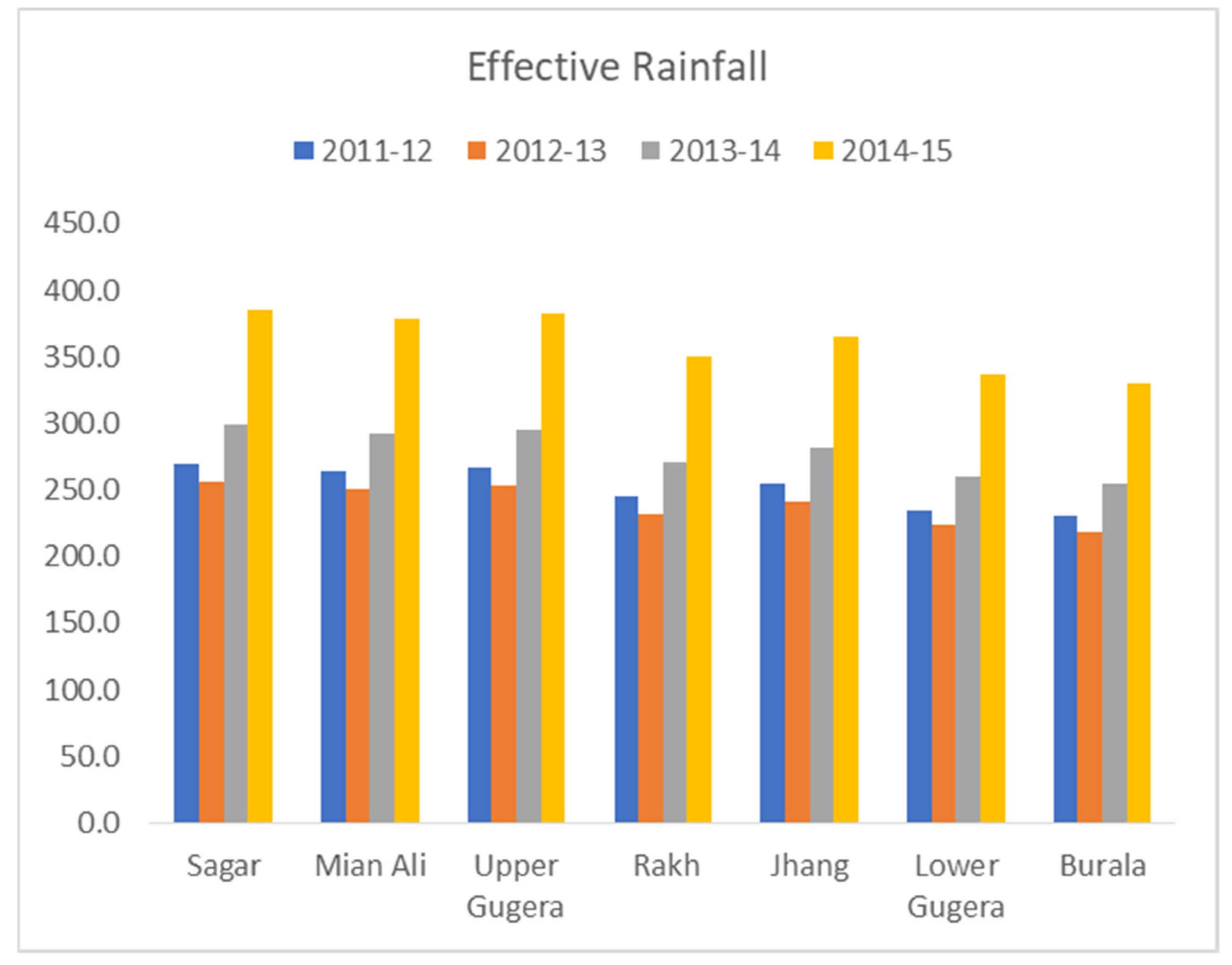
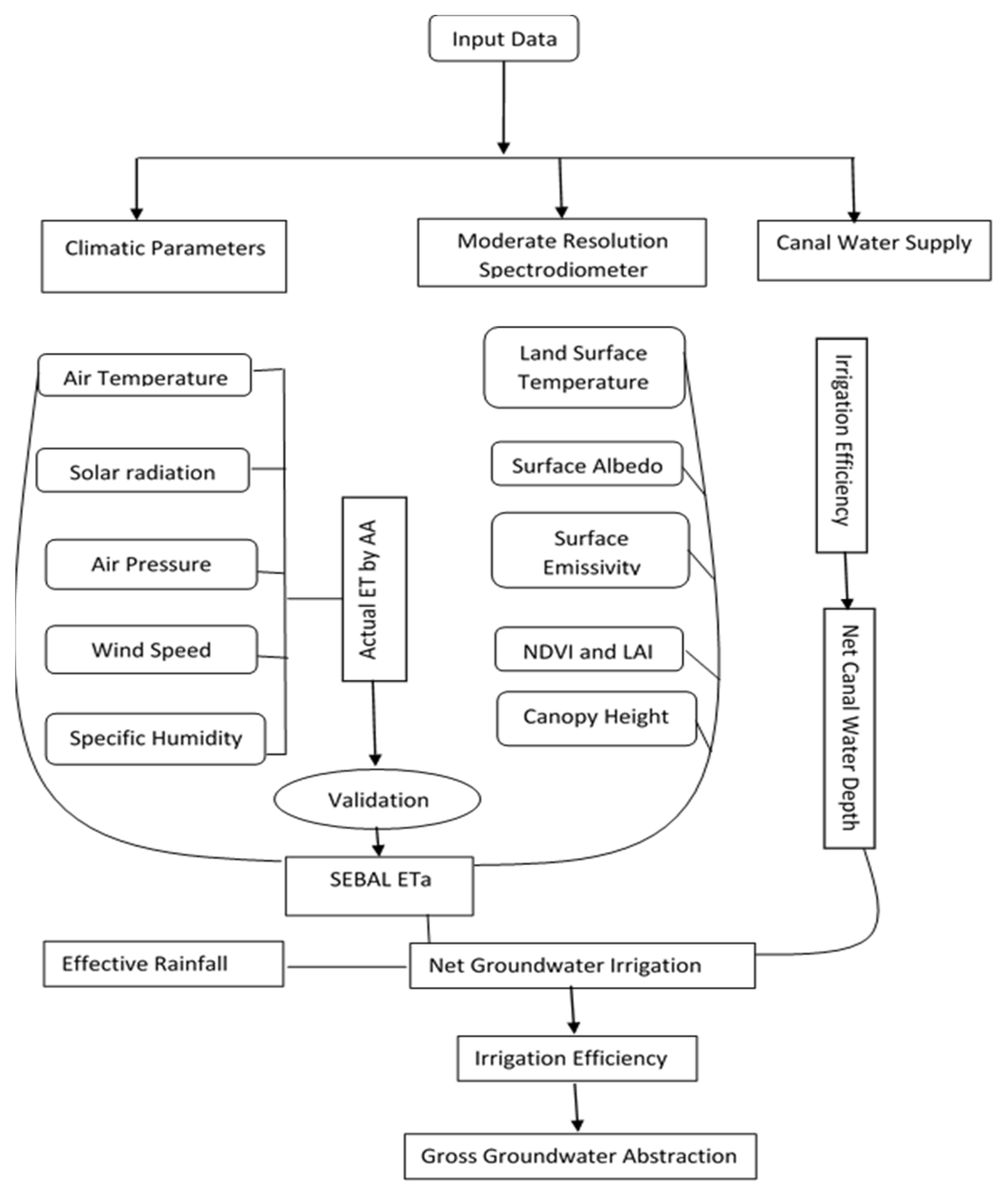
One of the largest contiguous irrigation systems in the world is only covered with 96 metrological stations, and only three metrological stations cover the Lower Chenab Canal System. Effective and reliable estimation of actual evapotranspiration is not possible through the empirical models for the very fine assessment of irrigation water management components. SEBAL is the most reliable and effective technique applied in different irrigation systems for the estimation of actual evapotranspiration. SEBAL was successfully applied in the different regions of the world for the estimation of the actual evapotranspiration [16,44,50,51]. The gross canal water availability in the irrigation system described the quantity of water available from the irrigation sources, while the net canal water availability described the actual amount of water available in the field after the exclusion of the system losses. Irrigation system efficiency was about 45% from the point of water diversion from the river to the point of application in the field. Estimation of effective rainfall described the amount of water available as a supplementary source of irrigation and reduced the demand for irrigation. The gross groundwater recharge was the amount of water that percolated due to the excessive irrigation from the canal system and the rainfall. This study was very comprehensive about the irrigation water management components and can help the policymakers effectively utilize the irrigation sources by reducing losses and improving effective irrigation scheduling by raising the flexibility. Remotely sensed data are acquired instantaneously and can only provide the instantaneous two-dimensional spatial distribution of land surface variables such as surface albedo, surface vegetation fraction, surface temperature, surface net radiation, soil moisture, etc., which are indispensable variables to know for remote sensing estimates of land surface ET. The methodology developed for the evaluation of irrigation water management components cannot evaluate short-term dynamics. The satellite data retrieved from the sources had a temporal resolution of 8 days and considered the cumulative effect; the daily change in the crop phenology was not considered. The method was found suitable and was widely applied for irrigation system management to develop crop combination maps, rainfall mapping, actual evapotranspiration mapping, and groundwater mapping where data scarcity is the main concern [20,25,44,52,53,54]. The method is not limited to the model framework chosen here; it also has application in the dry areas irrigation systems such as India, Egypt, and African countries. The current methods cover the issue of data scarcity and provide a suitable solution for mapping the irrigation water management components at a very fine resolution. The key parameters involved in this study were the retrieval of the MODIS data with 8 days temporal and 250 m spatial resolution as well as the daily discharge data from the irrigation system and the retrieval of rainfall at very fine temporal and spatial resolution of TRMM. The study provided a very fine estimation of the irrigation water management components. Rainfall was estimated based on the study performed by the [20] at basin scale. Actual evapotranspiration was estimated using SEBAL [16] for the equity assessment at the very fine spatial scale of canal command area.

5. Conclusions

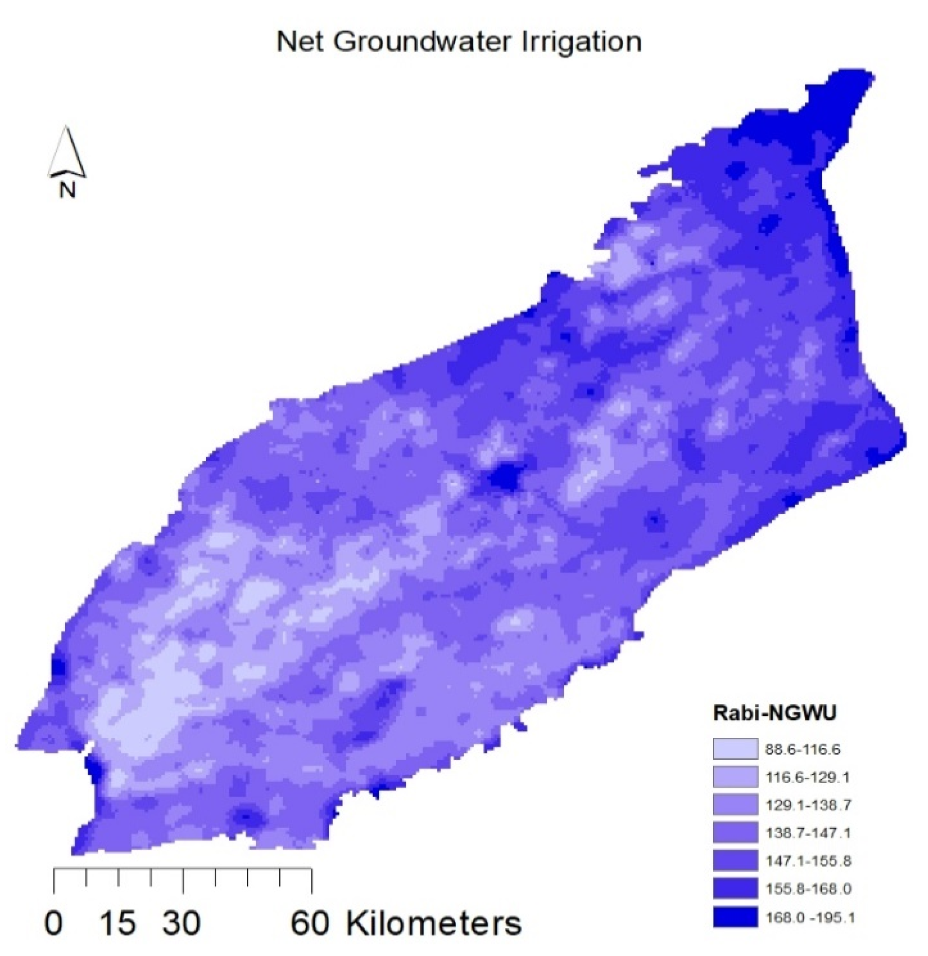
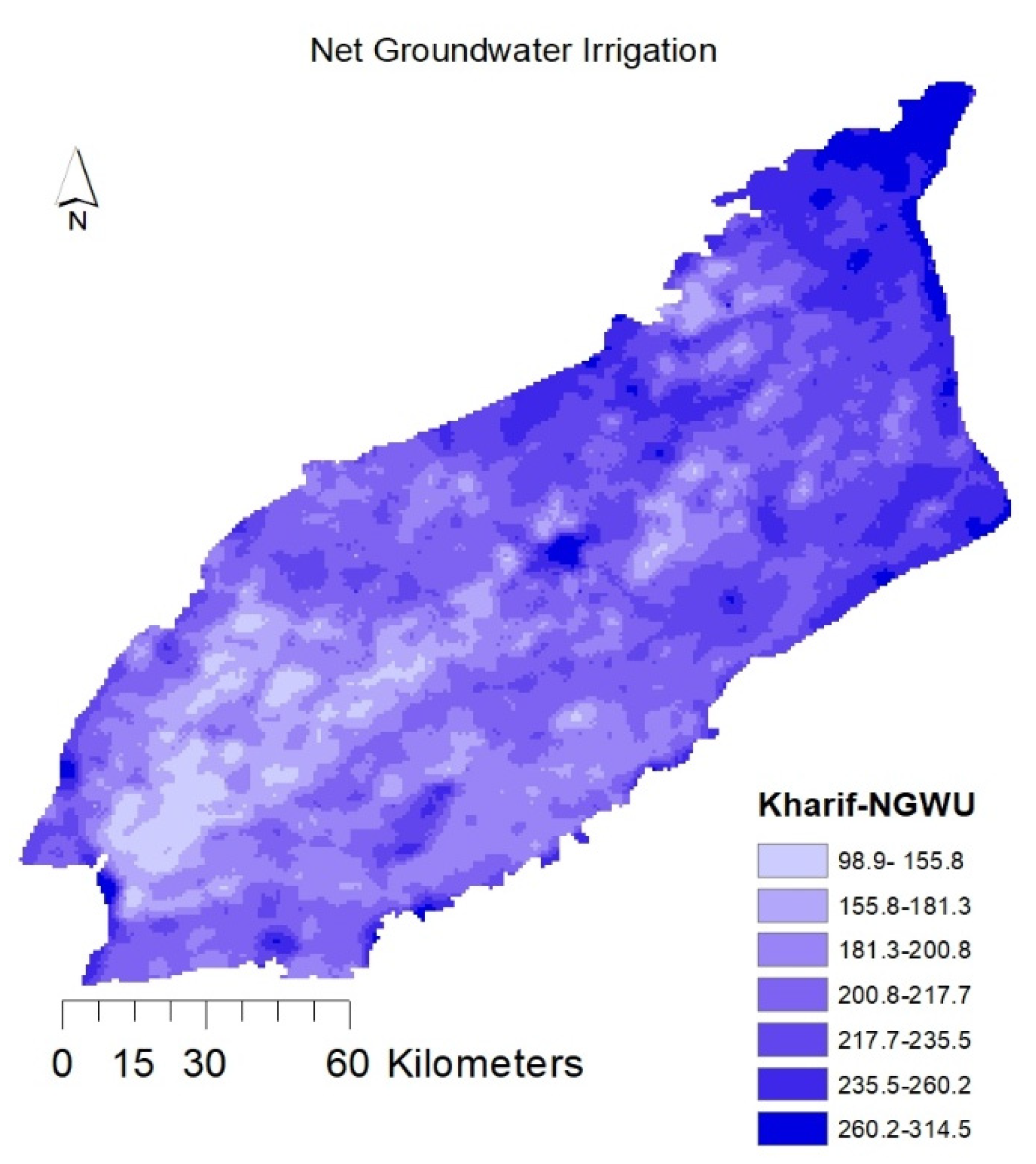
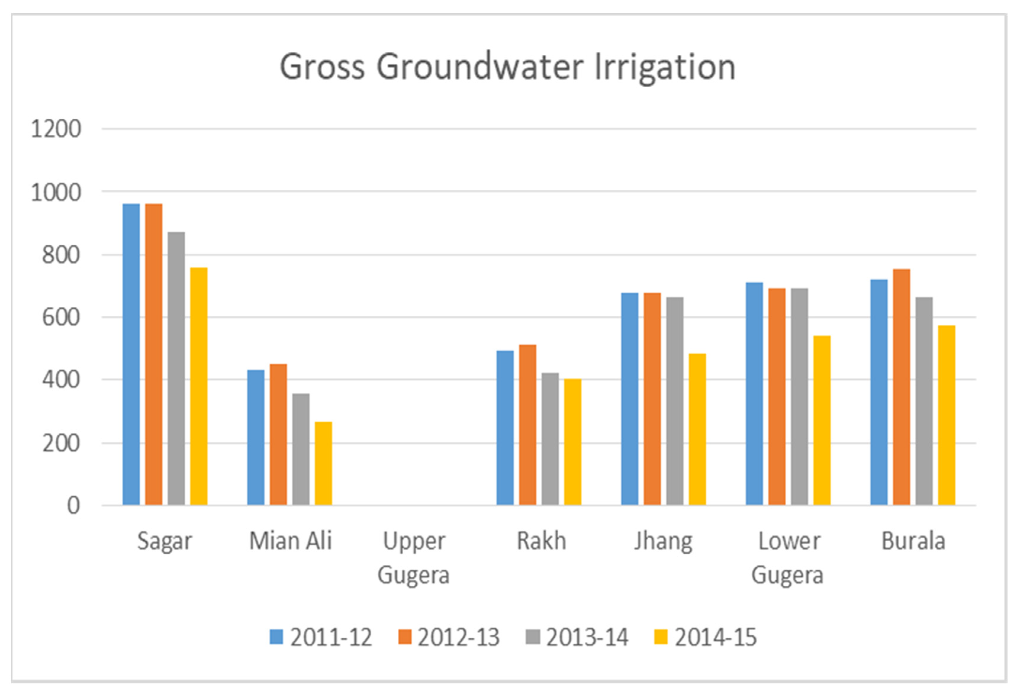
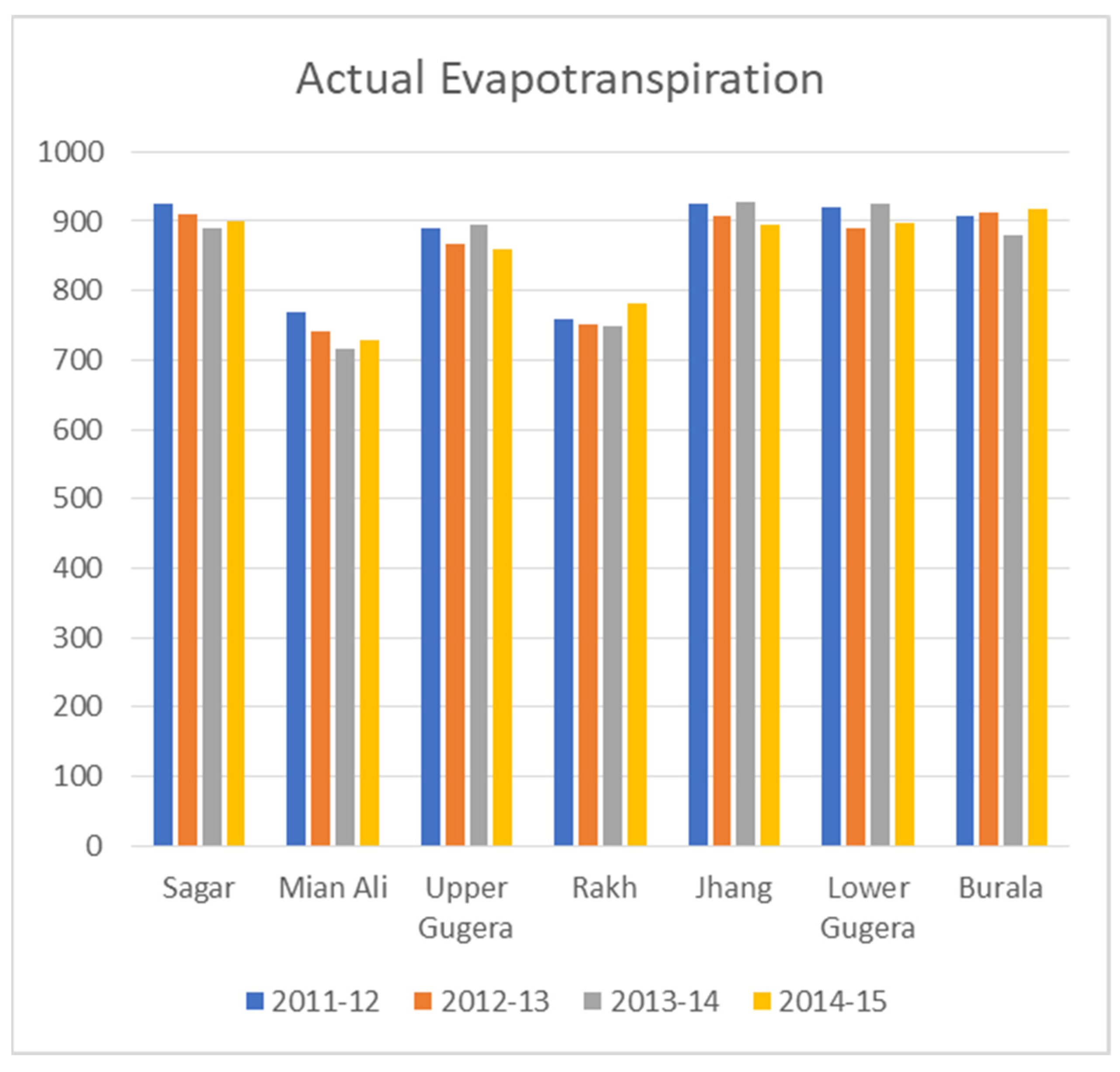
Four year average annual based actual evapotranspiration of 899 mm described the actual water requirement for the crop production. The water availability from the rainfall and the canal irrigation system during the four year study period only was 548 mm, which was only 36% of actual evapotranspiration. The contributions of the most flexible water resources of groundwater were 39% and 61% during Rabi and Kharif seasons. The most important resources of surface water supply variation at different scales were assessed for effective management. The spatial analysis of the system at canal command areas of the distributaries revealed the highest canal water availability at the Upper Gogera canal command and the lowest at the Sagar canal command. Therefore, groundwater extraction was found at its maximum at Sagar command due to less supply and cultivation of the high irrigation demanding crop (rice). Similarly, Jhang canal command, Burala canal command, and lower Goger canal command showed significant groundwater irrigation. Based on the study period, this study focused seriously on water allocation plans to avoid water logging in some areas and higher chances of secondary salinization in the major portion of the study area. It directed the water managers for the effective management of canal water resources to sustain soil and water productivity of the system for contribution in the achievement of sustainable development goals, as the rainfall occurrence is the uncontrolled resource, and groundwater is the most flexible water resource of the system.

References

1. Boelee, E.; Atapattu, S.; Amede, T. Ecosystems for Water and Food Security. 2011. Available online: http://www.iwmi.cgiar.org/Topics/Ecosystems/PPT/Ecosystems (accessed on 3 March 2021).
2. Jurriëns, M.; Mollinga, P.P.; Wester, P. Scarcity by Design: Protective Irrigation in India and Pakistan; ILRI: Nairobi, Kenya, 1996; ISBN 9070754401. [Google Scholar]
3. Bandaragoda, D.J.; Badruddin, M. Moving Towards Demand-Based Operations in Modernized Irrigation Systems in Pakistan; International Water Management Institute: Gujarat, India, 1992. [Google Scholar]
4. Ullah, M.K.; Habib, Z.; Muhammad, S. Spatial Distribution of Reference and Potential Evapotranspiration Across the INDUS Basin Irrigation Systems; IWMI: Gujarat, India, 2001; Volume 24, ISBN 929090206X. [Google Scholar]
5. Latif, M.; Ahmad, M.Z. Groundwater and soil salinity variations in a canal command area in Pakistan. Irrig. Drain. J. Int. Comm. Irrig. Drain. 2009, 58, 456–468. [Google Scholar] [CrossRef]
6. Hussain, I.; Hussain, Z.; Sial, M.H.; Akram, W.; Farhan, M.F. Water balance, supply and demand and irrigation efficiency of Indus Basin. Pak. Econ. Soc. Rev. 2011, 49, 13–38. [Google Scholar]
7. Navalawala, B.N. Water Scenario in India. Yojana Oct. 1995, 1, 5–11. [Google Scholar]
8. Sarwar, A.; Eggers, H. Development of a conjunctive use model to evaluate alternative management options for surface and groundwater resources. Hydrogeol. J. 2006, 14, 1676–1687. [Google Scholar] [CrossRef]
9. Qureshi, A.S.; McCornick, P.G.; Sarwar, A.; Sharma, B.R. Challenges and prospects of sustainable groundwater management in the Indus Basin, Pakistan. Water Resour. Manag. 2010, 24, 1551–1569. [Google Scholar] [CrossRef] [Green Version]
10. Yu, W.; Yang, Y.-C.; Savitsky, A.; Alford, D.; Brown, C.; Wescoat, J.; Debowicz, D.; Robinson, S. The Indus Basin of Pakistan: The Impacts of Climate Risks on Water and Agriculture; The World Bank: Washington, DC, USA, 2013; ISBN 0821398741. [Google Scholar]
11. Laghari, A.N.; Vanham, D.; Rauch, W. The Indus basin in the framework of current and future water resources management. Hydrol. Earth Syst. Sci. 2012, 16, 1063. [Google Scholar] [CrossRef] [Green Version]
12. Ahmad, M.-D.; Turral, H.; Nazeer, A. Diagnosing irrigation performance and water productivity through satellite remote sensing and secondary data in a large irrigation system of Pakistan. Agric. Water Manag. 2009, 96, 551–564. [Google Scholar] [CrossRef]
13. Kirby, M.; Mainuddin, M.; Khaliq, T.; Cheema, M.J.M. Agricultural production, water use and food availability in Pakistan: Historical trends, and projections to 2050. Agric. Water Manag. 2017, 179, 34–46. [Google Scholar] [CrossRef]
14. Liaqat, U.W.; Choi, M.; Awan, U.K. Spatio-temporal distribution of actual evapotranspiration in the Indus Basin Irrigation System. Hydrol. Process. 2015, 29, 2613–2627. [Google Scholar] [CrossRef]
15. Qureshi, A.S.; Shah, T.; Akhtar, M. The Groundwater Economy of Pakistan; IWMI: Gujarat, India, 2003; Volume 64, ISBN 9290905301. [Google Scholar]
16. Stisen, S.; Soltani, M.; Mendiguren, G.; Langkilde, H.; Garcia, M.; Koch, J. Spatial Patterns in Actual Evapotranspiration Climatologies for Europe. Remote Sens. 2021, 13, 2410. [Google Scholar]
17. Hertzog, T.; Poussin, J.-C.; Tangara, B.; Kouriba, I.; Jamin, J.-Y. A role playing game to address future water management issues in a large irrigated system: Experience from Mali. Agric. Water Manag. 2014, 137, 1–14. [Google Scholar] [CrossRef]
18. Ahmad, M.-D. Estimation of Net Groundwater Use in Irrigated River Basins Using Geo-Information Techniques: A Case Study in Rechna Doab, Pakistan; Wageningen University: Wageningen, The Netherlands, 2002; ISBN 9058087611. [Google Scholar]
19. Singh, R.; Kroes, J.G.; van Dam, J.C.; Feddes, R.A. Distributed ecohydrological modelling to evaluate the performance of irrigation system in Sirsa district, India: I. Current water management and its productivity. J. Hydrol. 2006, 329, 692–713. [Google Scholar] [CrossRef]
20. Cheema, M.J.M.; Bastiaanssen, W.G.M. Local calibration of remotely sensed rainfall from the TRMM satellite for different periods and spatial scales in the Indus Basin. Int. J. Remote Sens. 2012, 33, 2603–2627. [Google Scholar] [CrossRef]
21. Usman, M.; Liedl, R.; Awan, U.K. Spatio-temporal estimation of consumptive water use for assessment of irrigation system performance and management of water resources in irrigated Indus Basin, Pakistan. J. Hydrol. 2015, 525, 26–41. [Google Scholar] [CrossRef]
22. Liaqat, U.W.; Awan, U.K.; McCabe, M.F.; Choi, M. A geo-informatics approach for estimating water resources management components and their interrelationships. Agric. Water Manag. 2016, 178, 89–105. [Google Scholar] [CrossRef] [Green Version]
23. Usman, M.; Mahmood, T.; Conrad, C.; Bodla, H.U. Remote Sensing and Modelling Based Framework for Valuing Irrigation System Efficiency and Steering Indicators of Consumptive Water Use in an Irrigated Region. Sustainability 2020, 12, 9535. [Google Scholar] [CrossRef]
24. Awan, U.K.; Anwar, A.; Ahmad, W.; Hafeez, M. A methodology to estimate equity of canal water and groundwater use at different spatial and temporal scales: A geo-informatics approach. Environ. Earth Sci. 2016, 75, 409. [Google Scholar] [CrossRef]
25. Waqas, M.M.; Awan, U.K.; Cheema, M.J.M.; Ahmad, I.; Ahmad, M.; Ali, S.; Shah, S.H.H.; Bakhsh, A.; Iqbal, M. Estimation of Canal Water Deficit Using Satellite Remote Sensing and GIS: A Case Study in Lower Chenab Canal System. J. Indian Soc. Remote Sens. 2019, 47, 1–10. [Google Scholar] [CrossRef]
26. Awan, U.K.; Tischbein, B.; Martius, C. Combining hydrological modeling and GIS approaches to determine the spatial distribution of groundwater recharge in an arid irrigation scheme. Irrig. Sci. 2013, 31, 793–806. [Google Scholar] [CrossRef]
27. Conrad, C.; Dech, S.W.; Hafeez, M.; Lamers, J.; Martius, C.; Strunz, G. Mapping and assessing water use in a Central Asian irrigation system by utilizing MODIS remote sensing products. Irrig. Drain. Syst. 2007, 21, 197–218. [Google Scholar] [CrossRef] [Green Version]
28. Conrad, C.; Rahmann, M.; Machwitz, M.; Stulina, G.; Paeth, H.; Dech, S. Satellite based calculation of spatially distributed crop water requirements for cotton and wheat cultivation in Fergana Valley, Uzbekistan. Glob. Planet. Chang. 2013, 110, 88–98. [Google Scholar] [CrossRef]
29. Hellegers, P.; Soppe, R.; Perry, C.J.; Bastiaanssen, W.G.M. Combining remote sensing and economic analysis to support decisions that affect water productivity. Irrig. Sci. 2009, 27, 243–251. [Google Scholar] [CrossRef]
30. Hafeez, M.M.; Khan, S. Spatial mapping of actual crop water use in ground water dominant irrigation system. Aust. J. Agric. Res. 2007, 1, 1–50. [Google Scholar]
31. Bastiaanssen, W.G.M.; Ahmad, M.; Chemin, Y. Satellite surveillance of evaporative depletion across the Indus Basin. Water Resour. Res. 2002, 38, 1–9. [Google Scholar] [CrossRef]
32. Bandara, K.M.P.S. Assessing Irrigation Performance by Using Remote Sensing; Wageningen University: Wageningen, The Netherlands, 2006; ISBN 9085044065. [Google Scholar]
33. Xu, C.-Y.; Singh, V.P. Evaluation of three complementary relationship evapotranspiration models by water balance approach to estimate actual regional evapotranspiration in different climatic regions. J. Hydrol. 2005, 308, 105–121. [Google Scholar] [CrossRef]
34. Liu, S.; Sun, R.; Sun, Z.; Li, X.; Liu, C. Evaluation of three complementary relationship approaches for evapotranspiration over the Yellow River basin. Hydrol. Process. Int. J. 2006, 20, 2347–2361. [Google Scholar] [CrossRef]
35. Matin, M.A.; Bourque, C.P.-A. Assessing spatiotemporal variation in actual evapotranspiration for semi-arid watersheds in northwest China: Evaluation of two complementary-based methods. J. Hydrol. 2013, 486, 455–465. [Google Scholar] [CrossRef]
36. Usman, M.; Liedl, R.; Kavousi, A. Estimation of distributed seasonal net recharge by modern satellite data in irrigated agricultural regions of Pakistan. Environ. Earth Sci. 2015, 74, 1463–1486. [Google Scholar] [CrossRef]
37. Brutsaert, W.; Stricker, H. An advection-aridity approach to estimate actual regional evapotranspiration. Water Resour. Res. 1979, 15, 443–450. [Google Scholar] [CrossRef]
38. Priestley, C.H.B.; Taylor, R.J. On the assessment of surface heat flux and evaporation using large-scale parameters. Mon. Weather Rev. 1972, 100, 81–92. [Google Scholar] [CrossRef]
39. Penman, H.L. Natural evaporation from open water, bare soil and grass. Proc. R. Soc. London. Ser. A Math. Phys. Sci. 1948, 193, 120–145. [Google Scholar]
40. Bouchet, R.J. Evapotranspiration reelle, evapotranspiration potentielle, et production agricole. Ann. Agron. 1963, 14, 743–824. [Google Scholar]
41. Harmsen, E.W.; Mesa, S.E.G.; Cabassa, E.; Ramírez-Beltran, N.D.; Pol, S.C.; Kuligowski, R.J.; Vasquez, R. Satellite sub-pixel rainfall variability. Int. J. Syst. Appl. Eng. Dev. 2008, 2, 91–100. [Google Scholar]
42. Ahmad, M.-D.; Magagula, T.F.; Love, D.; Kongo, V.; Mul, M.L.; Kinoti, J. Estimating actual evapotranspiration through remote sensing techniques to improve agricultural water management: A case study in the transboundary Olifants catchment in the Limpopo basin, South Africa. In Proceedings of the 6th WaterNet/WARFSA/GWP Annual Symposium, Ezulwini, Swaziland, 1–4 November 2005. [Google Scholar]
43. Ahmad, M.; Bastiaanssen, W.G.M.; Feddes, R.A. Sustainable use of groundwater for irrigation: A numerical analysis of the subsoil water fluxes. Irrig. Drain. J. Int. Comm. Irrig. Drain. 2002, 51, 227–241. [Google Scholar] [CrossRef]
44. Awan, U.K.; Ismaeel, A. A new technique to map groundwater recharge in irrigated areas using a SWAT model under changing climate. J. Hydrol. 2014, 519, 1368–1382. [Google Scholar] [CrossRef]
45. Wilson, K.; Goldstein, A.; Falge, E.; Aubinet, M.; Baldocchi, D.; Berbigier, P.; Bernhofer, C.; Ceulemans, R.; Dolman, H.; Field, C. Energy balance closure at FLUXNET sites. Agric. For. Meteorol. 2002, 113, 223–243. [Google Scholar] [CrossRef] [Green Version]
46. Hobbins, M.T.; Ramirez, J.A.; Brown, T.C. The complementary relationship in estimation of regional evapotranspiration: An enhanced advection-aridity model. Water Resour. Res. 2001, 37, 1389–1403. [Google Scholar] [CrossRef] [Green Version]
47. Qureshi, A.S.; Gill, M.A.; Sarwar, A. Sustainable groundwater management in Pakistan: Challenges and opportunities. Irrig. Drain. J. Int. Comm. Irrig. Drain. 2010, 59, 107–116. [Google Scholar] [CrossRef]
48. Islam, M.N.; Uyeda, H. Vertical variations of rain intensity in different rainy periods in and around Bangladesh derived from TRMM observations. Int. J. Climatol. J. R. Meteorol. Soc. 2008, 28, 273–279. [Google Scholar] [CrossRef]
49. Chokngamwong, R.; Chiu, L. TRMM and Thailand daily gauge rainfall comparison. In Proceedings of the Preprints, 20th Conference on Hydrology, Atlanta, GA, USA, 27 January–3 February 2006; American Meteorological Society: Boston, MA, USA, 2006; Volume 1. [Google Scholar]
50. Zwart, S.J.; Bastiaanssen, W.G.M.; de Fraiture, C.; Molden, D.J. WATPRO: A remote sensing based model for mapping water productivity of wheat. Agric. Water Manag. 2010, 97, 1628–1636. [Google Scholar] [CrossRef]
51. Zwart, S.J.; Bastiaanssen, W.G.M. SEBAL for detecting spatial variation of water productivity and scope for improvement in eight irrigated wheat systems. Agric. Water Manag. 2007, 89, 287–296. [Google Scholar] [CrossRef]
52. Cheema, M.J.M.; Immerzeel, W.W.; Bastiaanssen, W.G.M. Spatial quantification of groundwater abstraction in the irrigated Indus basin. Groundwater 2014, 52, 25–36. [Google Scholar] [CrossRef] [PubMed] [Green Version]
53. Cheema, M.J.M.; Bastiaanssen, W.G.M. Land use and land cover classification in the irrigated Indus Basin using growth phenology information from satellite data to support water management analysis. Agric. Water Manag. 2010, 97, 1541–1552. [Google Scholar] [CrossRef]
54. Karimi, P.; Bastiaanssen, W.G.M.; Molden, D.; Cheema, M.J.M. Basin-wide water accounting based on remote sensing data: An application for the Indus Basin. Hydrol. Earth Syst. Sci. 2013, 17, 2473–2486. [Google Scholar] [CrossRef] [Green Version]
Figure 1. Lower Chenab canal command area.
Sustainability 13 08607 g001
Figure 2. The methodological framework for the quantification of groundwater irrigation.
Sustainability 13 08607 g002
Figure 3. Gross canal water distribution at the CCAs of the LCC system.
Sustainability 13 08607 g003
Figure 4. Comparison of satellite-based ETa and ETa by the AA method based calibration (2011–2012 to 2012–2013) and validation (2013–2014 to 2014–2015) of SEBAL.
Sustainability 13 08607 g004
Figure 5. Four years average SEBAL estimated ETa of the Rabi season.
Sustainability 13 08607 g005
Figure 6. Four years average SEBAL estimated ETa of the Kharif season.
Sustainability 13 08607 g006
Figure 7. Actual evapotranspiration at different CCAs of LCC.
Sustainability 13 08607 g007
Figure 8. Four years average Rabi season satellite derived rainfall.
Sustainability 13 08607 g008
Figure 9. Four years average Kharif season satellite derived rainfall.
Sustainability 13 08607 g009
Figure 10. Effective annual rainfall at CCAs (2011–2012 to 2014–2015).
Sustainability 13 08607 g010
Figure 11. Four years average Rabi season groundwater irrigation in the LCC.
Sustainability 13 08607 g011
Figure 12. Four years average Kharif season groundwater irrigation in the LCC.
Sustainability 13 08607 g012
Figure 13. Gross groundwater irrigation at different CCAs of the LCC system.
Sustainability 13 08607 g013