Article

Spatial-Temporal Evolution and Relationship between Urbanization Level and Ecosystem Service from a Dual-Scale Perspective: A Case Study of the Pearl River Delta Urban Agglomeration

1
School of Geography, South China Normal University, Guangzhou 510000, China
2
Institute of Economics, Shanghai Academy of Social Sciences, Shanghai 200030, China
*
Author to whom correspondence should be addressed.
Sustainability 2021, 13(15), 8537; https://doi.org/10.3390/su13158537
Submission received: 27 June 2021 / Revised: 22 July 2021 / Accepted: 23 July 2021 / Published: 30 July 2021

Abstract

:
Since the beginning of the 21st century, urbanization has brought about dramatic changes in population, life, and economy, while having a significant impact on the distribution of ecosystem service. As research on the relationship between urbanization and ecosystem service has gradually specified, we decided to explore it at different scales. In this paper, we quantified and mapped the spatial–temporal evolution and relationship between urbanization and ecosystem service value in the Pearl River Delta Urban Agglomeration from 2000 to 2019 based on a dual-scale perspective of county and 3 km × 3 km raster. Our results show that the overall trend of urbanization level and ecosystem service value was increasing. Urbanization and ecosystem service value at the county scale showed a negative spatial correlation, while it was not significant at the raster scale. The “high–high” agglomeration was more concentrated, while the other three “low–low”, “low–high” and “high–low” agglomerations were more dispersed. Our findings suggest it is crucial to identify the key factors of small urban areas to grasp the development mechanism in the urbanization process and maintain the balance of the ecosystem.

1. Introduction

Since the beginning of the 21st century, urbanization has been accelerating, which has led to ecological damage and other problems while promoting rapid development of society, economy, life, and culture. Urbanization in a narrow sense refers to the transfer of rural population to urban areas; urbanization in a broad sense includes the urbanization process of population, economy, society, natural ecology and land [1], and the urbanization discussed in this paper focuses on the broad sense. Ecosystem Service (ES) is the direct or indirect benefits that humans obtain from ecosystem [2,3], including tangible and intangible services that contribute to human survival and quality of life [3], which is important for maintaining urbanization development. After studying the impact of urbanization on the structure and function of wetland forests, Faulkne [4] found that urbanization development changes regional ecosystem service functions. Kreuter [5] obtained from a coupled perspective that urbanization changes the ecosystem service by changing land cover and natural land use. Therefore, it is important to understand the spatial–temporal relationship between urbanization and ecosystem service to coordinate regional sustainable development.
At present, the research on quantitative assessment of ecosystem service value (ESV) is improving, mainly including the comprehensive indicator assessment method [6], the value quantity method [7] and the energy value analysis method [8], among which the equivalent factor assessment in the value quantity method is the most widely used [9]. The evaluation of urbanization level has always received academic attention, but there is no more unified measurement method yet, mainly two kinds of single-type indicator and composite indicator, among which single-type indicator is simple to operate and easy to compare, including urbanization rate, population density, etc., and ignore the changes of economic industries and lifestyles in the process of urbanization cannot reflect the level of urbanization comprehensively [10]; composite one is mainly obtained by establishing the evaluation index system, selecting the factors and determining the weights and calculating the composite index through various measurement models [11]. Paul [12] established an evaluation index system covering 16 aspects such as population, employment, residence and distance from urban centers to evaluate the development of urbanization in the UK; Yukio Inaga [13] established an index system including town size, economic activity, employment, population and location conditions and proposed the concept of urbanity. Chinese urbanization started late. Chinese scholars only began to study the issue of urbanization patterns in China in the 1970s [14], among which Wang [15] constructed an index system for evaluating the quality of population and land urbanization, taking the Shandong Peninsula urban agglomeration as an example; Wang [16] measured the urbanization of the central Jilin urban agglomeration in four aspects, including population, economy, landscape environment, and lifestyle urbanization, from 2003–2013 comprehensive urbanization and suburbanization level; Jin [17] studied the quality of county urbanization development in Hubei province in 2009 and 2017 from 5 aspects of population, land, social, economic and urban-rural coordinated development urbanization; Ma [18] constructed the comprehensive urbanization level of five Central Asian countries from 4 aspects of population, economy, society and space. In urbanization evaluation studies, demographic, economic, living, social, ecological and land urbanization are the focus of research.
The above studies have laid a good foundation for a deeper understanding of the computational analysis of urbanization and the ecosystem service value, but there is a deficiency in the spatial relationship between them. In terms of research content, previous studies on urbanization process mainly focus on the influence of economy [19], knowledge [20], and policy [21], and few scholars pay attention to its role with ecosystem service, while studies on the response of ecosystem service also focus on landscape pattern [22,23], land use cover change [24], less associated with urbanization. In terms of research area, the number of studies related to districts and counties [25] has gradually increased in recent years, but few scholars have studied the spatial relationship between urbanization and ecosystem service value in a dual-scale perspective, especially raster scale [26]. Therefore, this paper measures the spatial–temporal evolution of ecosystem service value, individual and comprehensive urbanization levels of the Pearl River Delta Urban Agglomeration (PRD) based on a dual-scale perspective of county and raster, using socioeconomic, night lighting and land use/cover data for five periods of 2000, 2005, 2010, 2015 and 2019. Pearson correlation analysis and bivariate Moran’s I index are used to study the spatial relationship between urbanization and ecosystem service value to coordinate urbanization development and ecosystem conservation, with a view to providing a scientific basis for the spatially sustainable development of ecosystem service in urban procession.

2. Data and Methods

2.1. Overview of the Study Area and Data Sources

The Pearl River Delta Urban Agglomeration (21°25′ N–24°30′ N, 111°12′ E-115°35′ E), hereinafter referred to as “PRD”, is in the south of China. It consists of Guangzhou City, Shenzhen City, Zhuhai City, Foshan City, Dongguan City, Zhongshan City, Huizhou City, Jiangmen City and Zhaoqing City, adjacent to the two Special Administrative Regions of Hong Kong and Macau. The topography is complex and diverse, with hills and plains dominating the landscape, of which the highest elevation is 1363 m in the north of the South Ridge and the plains are mostly below 100 m. Located in the lower reaches of the Pearl River, it belongs to the southern subtropical maritime monsoon climate and covers an area of about 56,500 km2. Since the reform and opening up, the urbanization of the PRD has developed rapidly, with the urbanization rate of core area reaching 86.28%, per capita GNP of 160,000 yuan and a population density of 1212 people/km2 at the end of 2019. As the most densely populated urban agglomeration in the country, the ecosystem of PRD has been fragmented by urbanization and the differences in population density and socioeconomic development have exacerbated the uneven development of the region, presenting significant spatial differences. The coordination of urbanization and ecosystem service has become increasingly prominent.
Three types of spatial and statistical data are used in this study. First, land use/cover data for five years of 2000, 2005, 2010, 2015 and 2019 include cropland, forest land, grassland, water body, construction land and unused land with resolution of 30 m × 30 m, which are obtained from the Resource and Environmental Science Data Center of the Chinese Academy of Sciences (http://www.resdc.cn). Secondly, demographic, social and economic data are obtained from Guangdong Provincial Statistical Yearbook, China County Statistical Yearbook and related city and county statistic yearbook. Finally, the third type of data is the nighttime lighting data from the dataset of An extended time-series (2000–2018) of global NPP-VIIRS-like nighttime light data which were obtained from Harvard Dataverse Platform (https://dataverse.harvard.edu/dataset.xhtml?persistentId=doi:10.7910/DVN/YGIVCD) and has a ground resolution of 30 arc second. Considering the feature of China, all data are projected to WGS_1984_UTM_Zone_49N, clipped by the shape file of Pearl River Delta Urban Agglomeration and created to 3 km × 3 km raster with ArcGIS 10.2 to accumulate the level of urbanization and ecosystem service value. See Figure 1.
Note: The map is based on the standard map (review number GS (2016 2556)) downloaded from the standard map service website of the National Bureau of Surveying, Mapping and Geographic Information, with no modifications to the base map.

2.2. Caculation of Value of Ecosystem Service

The quantitative assessment of ecosystem service value is important for maintaining regional ecological security and promoting the coordinated development of regional economy and environment [27]. In this paper, the value of ecosystem service in the PRD is measured by the improved unit area value equivalent factor method of Xie [28]. Among them, the value of one standard unit ESV equivalent factor is equivalent to 1/7 of the average economic value of grain yields in the PRD (Equation (1)), which is calculated as
C = 1 7 * P * Q
where:
C = the value of one standard unit of ESV equivalent factor (yuan/hm2);
P = the average price of grain in the PRD;
Q = the grain yield per unit area in the PRD (kg/hm2).
To eliminate the interference of price fluctuations on value changes, this study introduces the Consumer Price Index (CPI) to adjust the average food price data of each year to the price level of 2019 [23,29], and uses the correction method of Xu [30] and Xie [31] for the equivalent factor table of the ecosystem per unit area. The economic value of the service function is corrected (Equations (2) and (3)) to derive the economic value of food production service provided per unit area of the farmland ecosystem, and finally the corrected ecosystem service value coefficient of the PRD. The calculation formula is:
λ = Q Q 0 * θ
E i = λ * E 0
where:
λ = the equivalent factor correction factor;
Q = the average grain yield per unit area in the PRD from 2000 to 2019 (kg/hm2);
Q 0 = the national annual average grain yield per unit area (kg/hm2);
θ = the biomass factor of farmland ecosystems in different provinces in China proposed by Xie Gaodi;
E i = the modified equivalent factor of land use type i;
E 0 = the equivalent factor of land use type determined by Xie.
The specific process is as follows: The average grain production in the PRD from 2000–2019 is 5291.3 kg/hm2 according to the Guangdong Provincial Statistical Yearbook. Based on the grain price statistics from the South China Grain Exchange, the 2019 PRD grain purchase price was estimated to be 2.55 yuan/kg. Using the CPI to adjust the average grain price data for each year to the 2019 price level, the value of 1 standard unit of ESV equivalent factor in the PRD in 2000, 2005, 2010, 2015 and 2019 was calculated 1278.28, 1369.8, 1873.29, 1928.07 and 1873.48 yuan/hm2, respectively. Based on the national agricultural land unit area grain yield of 5004.65 kg/hm2 and Guangdong Province land use type equivalent factor of 1.4, the correction coefficient of the PRD ecological service value equivalent factor table was obtained as 1.48, and then the land use/cover of the PRD was linked to the ecosystem type, in which the ecological service value generated by construction land was not considered for the time being, arable land corresponded to agricultural land, forest land corresponds to forest, beaches and mudflats in water bodies correspond to wetlands, and the corresponding value of desert is taken for unused land and multiplied by the ecological service value per unit equivalent to obtain a table of ecosystem service value factors suitable for the study area(Table 1). It shows that ecosystem service value coefficient per unit area is on the rise during the period of 2000–2015 and then decrease. Water body contributes more than any other land use types, followed by wetland and woodland, with over 300 thousand, 100 thousand and 50 thousand yuan, respectively.

2.3. Assessment of Urbanization Level

2.3.1. Constructing a Comprehensive Urbanization Level Evaluation System

It was found through the literature that demographic, economic, life, social, ecological and land urbanization are the main focus in urbanization evaluation studies. However, as ecological urbanization is more relevant to the ecosystem service involved in this study, the overlap between society and life is high but society does not cover as much as life, and land urbanization covers more aspects of life, economy, and population. To avoid contradictions in the later analysis and to consider the availability of data, this paper selects three aspects of life, economy and population to build a comprehensive urbanization level evaluation system for the Pearl River Delta Urban Agglomeration, which contains 8 specific indicators (Table 2).

2.3.2. Weighting Measurement Method

The entropy method is an objective assignment method, which calculates the index weights according to the dispersion degree of each index, the greater the dispersion degree of the index, the greater the influence of the index on the comprehensive evaluation, we adopt the entropy method to determine the index weights, and the calculation steps are as follows.
1
Standardization of original data.
Positive indicators:
S k i j = x k i j min ( x k i j ) max ( x i j ) min ( x i j )
Negative indicators:
S k i j = max ( x k i j ) x k i j max ( x k i j ) min ( x k i j )
x k i j = the value of the jth indicator in the ith district and county in year k;
min ( x k i j ) = the minimum value of indicators in all years in each district and county;
max ( x k i j ) = the maximum value of indicators in all years in each district and county.
2
Given r (k = 1, 2, ..., r) counties, m (I = 1, 2, ..., m) years, and n (j = 1, 2, ..., n) indicators, calculate the weight   y k i j of the value of the jth indicator in the ith year of kth county:
  y k i j = S k i j k = 1 r i = 1 m S k i j
3
Calculate the information entropy value e j for the jth indicator:
e j = 1 l n r m * k = 1 r i = 1 m * ( y k i j * l n y k i j ) .   ,
4
Calculation of indicator weights W j :
W j = g j j = 1 n g j ,   g j = 1 e j
5
Calculate the index score F j :
F j = j = 1 n ( W j * S k i j )
The index scores F j are calculated by Formula (9) to reflect the comprehensive urbanization level, life urbanization level, economy urbanization level and population urbanization level of each district or county, and the larger the value is, the higher the urbanization level is.

2.3.3. Spatialization of Comprehensive Urbanization Level

The level of urbanization is a comprehensive reflection of urbanization in terms of population, human activities, industry and economy, etc. The nighttime light data are a combined reflection of the results of the interaction of these factors, therefore, the integrated processed NPP-VIIRS-like nighttime light data are selected to correct the comprehensive urbanization level in this study, and the spatialization path of the comprehensive urbanization level is shown in Figure 2.
1
Modified construction of the light index reflecting the level of regional urbanization
The lighting index L i is constructed from two attributes of regional night lighting distribution to correct the comprehensive urbanization level: (i) regional average lighting intensity; (ii) regional lighting area. The two attributes are defined and calculated by the following indexes, and then linearly weighted to form the lighting index ( L i ), which is defined as a relative value to remove the influence of scale differences and to facilitate year-to-year comparisons.
L i = u * I i + v * S i
I i = ( M j * D j ) D m a x * M j
S i = M j A i
where
L i = the lighting index of region i;
  I i = the average light intensity indicator of region i, which characterizes the proportional relationship relative to the maximum possible light intensity;
S i = lighting area index of region i, which is defined as the total area of all lighting areas in the region (light intensity is not zero area) accounted for the proportion of the entire area, reflecting the extensibility of the light in space;
u , v ( u + v = 1) are the weights of I i and S i , which will be determined by the correlation analysis later on;
D j = the light intensity of the jth light area in region i;
M j = the area of the jth light area in region i;
D m a x = the maximum light intensity in the study area;
M j = the total area of all lighting areas in region i;
A i = the total area of region i.
2.
Correlation analysis of the light index and the comprehensive urbanization level of cities
In this study, the correlations between different nighttime lighting indices and comprehensive urbanization levels were calculated to determine the optimal lighting indices for the sub-districts, and modeling regression analysis was performed using the econometric software STATA16.0. Experimentally, it was proved that the correlation and fitting effect was best after logarithmic treatment of the variables, so the regression model as in Equation (13) was established after logarithmic transformation of the variables first.
ln ( U R i ) = a + b * l n ( u * I i + v * S i ) + ε i
where:
U R i = the comprehensive urbanization level of region i;
( u * I i + v * S i ) is the light index L i constructed in Equation (10);
ε i = the random error term in the model; and
a and b are the regression model coefficients.
Regression analysis of the weight combinations of different lighting indices yielded the following results for the fit (R2). As seen in Table 3, separate regressions were performed from the (0.1, 0.9) combination of weights to the (1, 0) combination, and the results showed the best fit at the (0.9, 0.1) combination, with an R2 of 0.81. The formula for the lighting index L i was thus determined as
L i = 0.9 * I i + 0.1 * S i
3.
Spatialization of comprehensive urbanization level
The comprehensive urbanization level of the raster is assigned to the corresponding raster after the coefficients are calculated based on the regression. Finally, the actual comprehensive urbanization level of each district and county is linearly adjusted with the predicted comprehensive urbanization level to correct the value of each raster, and the corrected comprehensive urbanization level of the PRD at the raster scale is generated with the following equations.
U R i = e a * ( 0.9 * I i + 0.1 * S i ) b
U R i c = U R i * U R i U R i *
Equation (15) is transformed from Equation (13), where:
U R i c = the comprehensive urbanization level of the raster after correcting for the actual comprehensive urbanization level;
U R i = the predicted comprehensive urbanization level of each raster;
U R i = the comprehensive urbanization level of the district and county to which the raster belongs;
U R i * = the predicted comprehensive urbanization level of the district and county to which the raster belongs.

2.4. Correlation Analysis of Urbanization Level and ESV

2.4.1. Pearson Correlation Analysis

Analyzing the correlation between single and comprehensive urbanization level and ecosystem service value can better reflect the mutual influence of urbanization and ecosystem service. In this study, the Spearman coefficients were calculated by STATA to identify the correlation between the comprehensive urbanization level (Compr_ur), population urbanization level (Pop_ur), economy urbanization level (Eco_ur), life urbanization level (Life_ur) and ecosystem service value (ESV) from 2000 to 2019, respectively. It can also be used to analyze the sensitivity of the correlation and explore the extent of its impact.

2.4.2. Bivariate Spatial Autocorrelation Analysis

Bivariate spatial autocorrelation analysis is a measure of whether multiple variables are clustered in a spatial distribution [35] and explains the correlation between the value of spatial unit attributes and the value of other attributes in its adjacent space, including two parts: global spatial autocorrelation and local spatial autocorrelation [25]. The global spatial autocorrelation is used to describe the degree and significance of spatial correlation between variables in the study area, and the local spatial autocorrelation can discern the aggregation effect of an element in space on the surrounding elements to achieve the study of the dynamics of local changes in space [36], and the calculation equations [37] are:
I = i = 1 n j = 1 n W i j ( x i x ¯ ) ( x j x ¯ ) S 2 ( i j W i j )
I i = ( x i x ¯ ) j = 1 n W i j ( x i x ¯ ) S 2 ,   S 2 = 1 n i = 1 n ( x i x ¯ ) 2
where
I = the global Moran’s I index;
I i = the local Moran’s I index;
    n = the number of spatial cells;
  x i , x j = the observed values of cell i and cell j , respectively;
  ( x i x ¯ ) = the deviation of the observed value on the ith spatial cell from the mean, W i j = the spatial weight value between cell i and cell j ; and
  S 2 is the variance.
In this paper, we used GeoDa1.14, a spatial analysis software, to establish a spatial distance weight matrix to analyze the spatial autocorrelation between comprehensive urbanization level and ecosystem service value in the PRD, and used LISA (Local indicators of Spatial association) distribution maps to explore the spatial correlation between the two and their spatial heterogeneity characteristics.

3. Results

3.1. Analysis of the Spatial–Temporal Evolution of ESV

3.1.1. Spatial–Temporal Evolution of ESV at County Scale

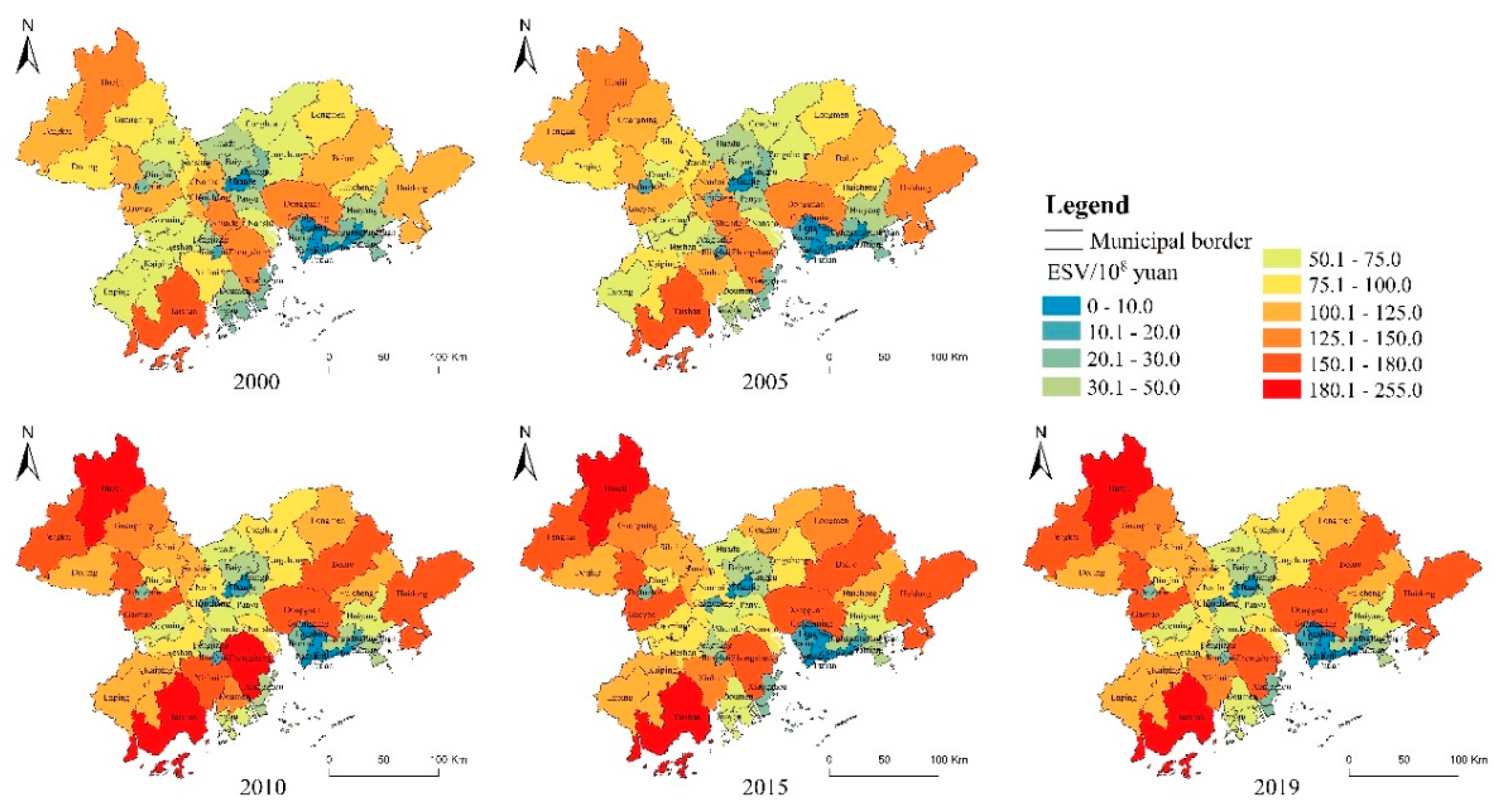
As shown in Figure 3, Table 4: (1) The value of ecosystem service in the PRD from 2000–2019 was 283.050 billion yuan, 298.551 billion yuan, 396.635 billion yuan, 391.355 billion yuan and 377.573 billion yuan, showing an overall trend of first increasing and then decreasing year by year, with an increase of 5.48% from 2000–2005, an increase from 2005–2010 by 32.85%, 2010–2015 decreased by 1.33%, and 2015–2019 decreased by 3.52%. (2) The high-value ESV areas in the PRD are widely distributed in the peripheral areas of the PRD, mainly in Taishan City and Huaiji County, with the highest ESV growth rate in Jinwan District and Yuexiu District in the past 20 years, 106.73% and 99.04% respectively. (3) The low value ESV areas in the PRD gathered in the central part of Guangzhou City and the northeast corner of Shenzhen City, namely Tianhe District, Yuexiu District and Liwan District in Guangzhou City and Futian District, Nanshan District and Luohu District in Shenzhen City, with the lowest growth rates of −58.07% and −56.74% in Chancheng District and Shunde District in the last 20 years, respectively. (4) From 2000–2010, the ESV of each county is dominated by a growth trend, with the highest growth rate of 55.11% in Jinwan District and the lowest growth rate of −30.89% in Baoan District during 2000–2005, and the highest growth rate of 140.6% in Doumen District and the lowest growth rate of −50.49% in Chancheng District during 2005–2010. During 2010–2019, increasing rate of ESV of most counties gradually declined, with the highest growth rate of 16.05% in Liwan District and the lowest growth rate of −42.9% in Doumen District during 2010–2015, and the highest growth rate of 7.43% in Guangming District and the lowest growth rate of −11.24% in Longhua District during 2015–2019. Since 2005, the highest growth rate value of each district and county has gradually decreased, and the difference has become smaller and smaller, especially between the highest and lowest values of its growth rate between year 2015 and 2019 is less than 20%, indicating that the overall trend tends to urbanization maturity.

3.1.2. Spatial–Temporal Evolution of the Raster Scale

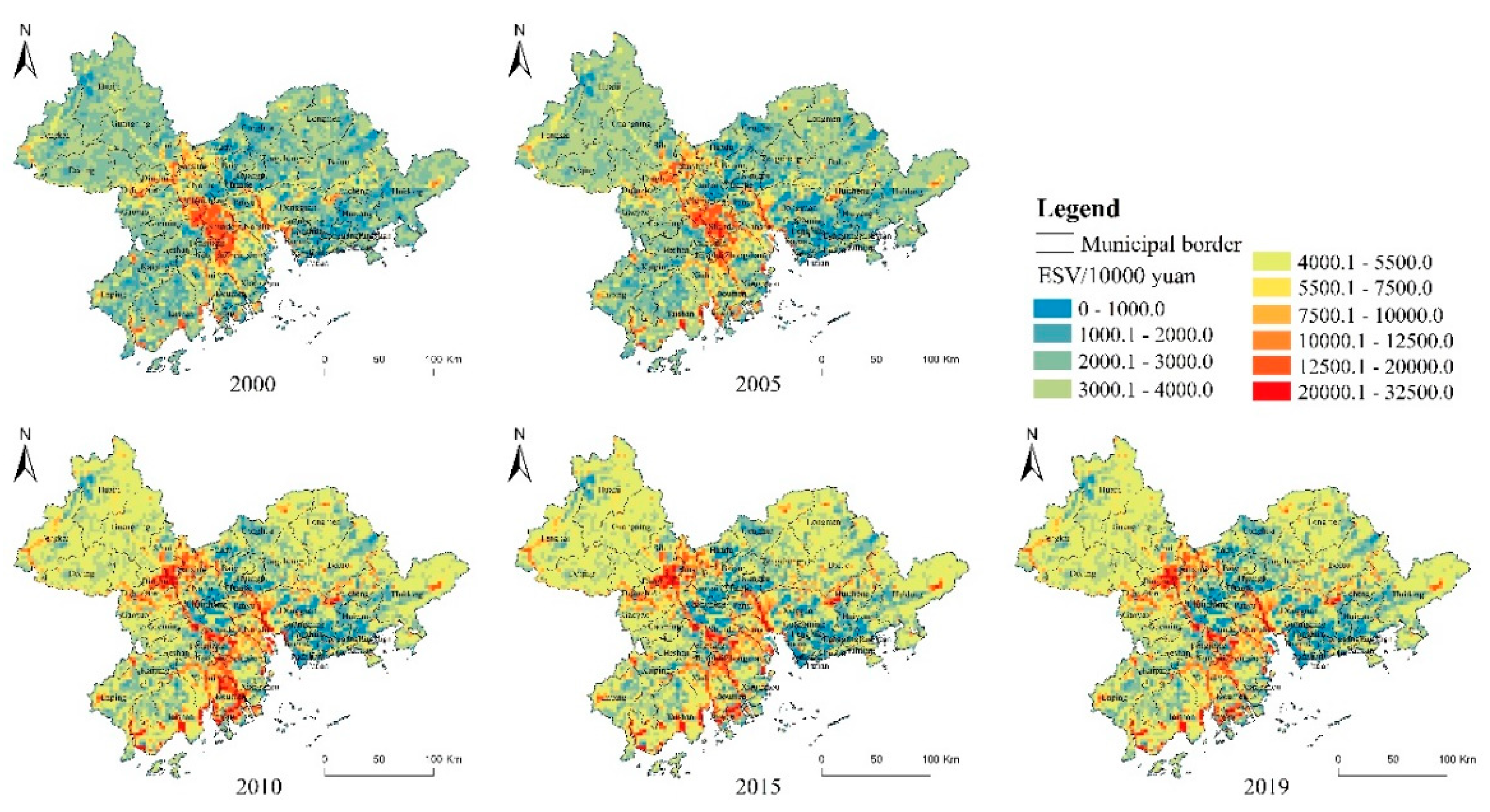
As seen in Figure 4: (1) The high ESV areas in the PRD during 2000–2005 were mainly distributed in the central part of the PRD, and underwent significant spatial changes from 2005–2010, shifting from the abdominal center to the northwest, southeast and southern regions, concentrating in Dinghu District and Sanshui District in the southeast of Zhaoqing City, Xinhui City in the northeast of Jiangmen City, Jinwan District in Zhuhai City, the border between Nansha District and Dongguan City in Panyu District, Pengjiang District, Zhongshan City and the border of Shunde District, etc. (2) The low ESV areas in the PRD were widely distributed in the west and east of the PRD during 2000–2005, and began to be concentrated in Shenzhen, Guangzhou and Foshan after 2010. (3) The spatial distribution of ESV in the PRD changed from high in the lowlands and low around in 2000 to a pattern of low in Guangzhou, Shenzhen and Foshan and high in Foshan with northwest, southeast and south in 2019, and spatial heterogeneity increased significantly.

3.2. Analysis of the Spatial–Temporal Evolution of Urbanization Level

3.2.1. Spatial–Temporal Evolution of Urbanization Level at County Scale

As seen in Figure 5 and Figure 6 (1) the comprehensive urbanization level of the PRD rose from 0.1532 to 0.5178 between 2000 and 2019, a 3.38-fold rise in rapid development over 20 years. In terms of individual urbanization levels, economy urbanization grew explosively from 0.0319 in 2000 to 0.3562 in 2019, an 11.2-fold increase. Within the same development stage, the population urbanization level increased from 0.0327 to 0.0563, and the life urbanization level increased from 0.0885 to 0.1053, showing a slow growth trend. Among them, the economy urbanization level of the PRD urban agglomeration is the fastest growing, and the comprehensive urbanization level ranks second, while the other two types of urbanization levels are relatively stable within the study period. (2) The high-value areas of the comprehensive urbanization level in the PRD are concentrated in the abdomen area of the PRD, and have a greater degree of intersection with the high-value areas of ESV, mainly in Tianhe District of Guangzhou, Futian District of Shenzhen, Nanshan District and other districts and counties in the past 20 years Huangpu District of Guangzhou, Tianhe District, Huadu District, Longgang District of Shenzhen and Dongguan City have higher growth rates of comprehensive urbanization level, 283.27%, 261.65%, 129.48%, 157.17% and 130.26% respectively. (3) Low value areas of comprehensive urbanization level in the PRD are widely distributed in the northwestern, southwestern and northeastern corners of the PRD, mainly in Zhaoqing City, Jiangmen City and Huidong County of Huizhou City, with lower growth rates of −49.24%, −34.48% and −26.18 for Taishan City of Jiangmen City, Enping City and Longmen County of Huizhou City in the past 20 years. (4) From 2000 to 2005, the district and county with the highest growth rate of comprehensive urbanization level was Huangpu District of Guangzhou City, which rose by 183.98%, and the lowest was Taishan City of Jiangmen City, which fell by 26.54%. From 2005 to 2010, the corresponding counties are Huaiji County of Zhaoqing City and Taishan City of Jiangmen City, up by 48.68% and down by 22.96% respectively; from 2010 to 2015, the corresponding counties are Tianhe District of Guangzhou City and Longmen County of Huizhou City, up by 110.73% and down by 6.17% respectively; from 2015 to 2019, the corresponding counties are Longgang District of Shenzhen City and Fengkai County of Zhaoqing City, up by 38.60% and down by 27.22% respectively Table 4.

3.2.2. Spatial–Temporal Evolution of the Raster Scale

As seen in Figure 7: (1) in 2000, the overall level of urbanization in the PRD was low and homogeneous; since 2005, two high-value areas gradually appeared in the PRD in the central Yuexiu District and Tianhe District of Guangzhou and Futian District of Shenzhen, and spread radially from two points to all around with the change of time; by 2019, the high-value areas expanded to Guangzhou, Shenzhen, Foshan, Dongguan, Zhongshan and the southwestern part of Huizhou City, the northeastern part of Jiangmen City. (2) The low value areas of the comprehensive urbanization level in the PRD are widely distributed in the periphery of the PRD and have continued to show a decreasing trend in the past 20 years. (3) The spatial differences in the comprehensive urbanization level in the PRD are significantly centripetal, especially the high value of significant expansion since 2005, the urbanization spillover effect in the central region drives the development of the surrounding areas, the spatial heterogeneity is strong, and the overall comprehensive urbanization level has increased significantly, showing a mature regional urbanization pattern.

3.3. Correlation between Comprehensive Urbanization Level and Ecosystem Service Value

3.3.1. Correlation Analysis of Urbanization Level and ESV

As shown in Table 5: Ecosystem service value shows negative correlation with comprehensive urbanization, population urbanization and economy urbanization, and positive correlation with life urbanization, respectively, and all correlations are significant at the level of 0.01. The degree of influence of urbanization development on ESV is strong. For each 1% increase in comprehensive, population and economy urbanization levels, ESV will decrease by 43.9, 53.9 and 28.1 ten thousand yuan, respectively, with population urbanization level having the greatest impact; for each 1% increase in life urbanization, ESV increases by 32.6 ten thousand yuan. The high life urbanization level motivated by the rising energy efficiency, people’s awareness of environment protection and advanced technology has promoted the environment protection which will greatly improve the ecosystem value. However, how specific factors affect ecosystem need more complex models to deduce, such as system dynamic, neural networks, etc.

3.3.2. Spatial Autocorrelation Analysis of Comprehensive Urbanization Level and ESV

  • Spatial–temporal changes at the county scale
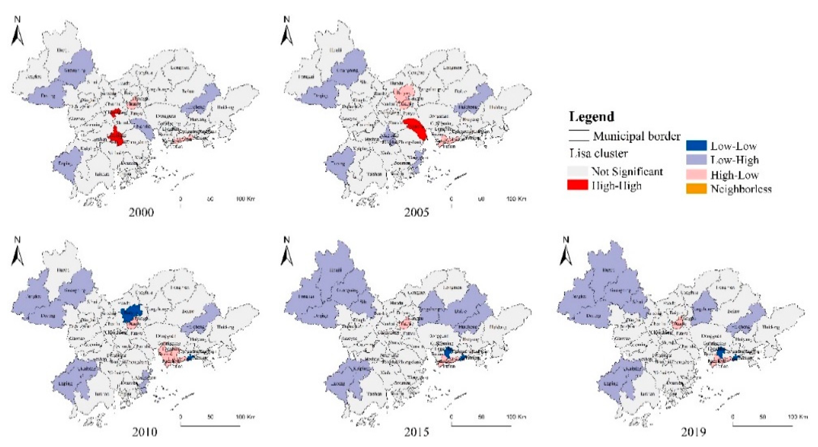
As seen in Table 6, Figure 8: (1) the global Moran I indices of integrated urbanization level and ecosystem service value from 2000 to 2019 are classified as −0.459, −0.447, −0.479, −0.435, and −0.467, with a negative correlation between the two in the past 20 years. (2) In 2000, the areas with “high–high” agglomeration of integrated urbanization level and ecosystem service value were Chancheng District, Pengjiang District and Jianghai District; the areas with “low–high” agglomeration were Deqing, Guangning County, Enping City, Nansha District and Huicheng District; the areas with “high–low” agglomeration were Tianhe District, Yuexiu District and Haizhu District of Guangzhou City and Nanshan District, Luohu District and Futian District of Shenzhen City. “High–Low” clustering areas are Tianhe District, Yuexiu District and Haizhu District of Guangzhou City and Nanshan District, Luohu District and Futian District of Shenzhen City, and “Low–Low” clustering does not reach 95% confidence level. In 2005, the “high–high” agglomeration area was Nansha District, the “low–high” agglomeration area increased by three—Pengjiang District, Jianghai District and Xiangzhou District—and decreased by one—Nansha District—the “high–low” agglomeration The overall change of “high–low” agglomeration is not significant, with the addition of Baiyun District and the reduction of Yantian District, and the "low–low" agglomeration still does not reach the 95% confidence level; in 2010, the “high–high” agglomeration did not reach the 95% confidence level. The overall number of “low–high” agglomeration areas remained unchanged, among which Pengjiang District and Jianghai District in 2005 were changed to Fengkai County and Kaiping County, and the number of “high–low” agglomeration areas increased by Baoan District and Longhua District and decreased by Baiyun District. The "low–low" agglomeration areas are Baiyun District and Yantian District. In 2015, the “high–high” agglomeration did not reach the 95% confidence level, and the “low–high” agglomeration expanded extensively. (3) From 2000 to 2005, the "low–low" agglomeration areas in the PRD did not reach the 95% confidence level, and the only significant agglomerations were "high–high," "low–high," and “high–low”. However, since 2010, the “high–high” agglomerations have disappeared and have been replaced by "low–low" agglomerations, indicating that the level of urbanization in the PRD has been increasing. Intense human activities have seriously damaged the ecological environment and resources, resulting in a significant reduction in the value of regional ecosystem service. (4) The “high–low” agglomeration areas are mainly located in the city centers of Guangzhou and Shenzhen, where Tianhe, Yuexiu and Haizhu districts of Guangzhou and Nanshan and Futian districts of Shenzhen have been in the “high–low” agglomeration in the past 20 years. These areas are in the plains, with a high concentration of humans and a high proportion of economic production. The strong human activities have led to the continuous improvement of the infrastructure construction in population, economy and life, and the increase of the comprehensive urbanization level, while destroying the local green space and water environment to a large extent, resulting in low ecosystem service value.(5) The “low–high” gathering areas are mainly located in Guangning County and Deqing County in the northwest of Zhaoqing City, Enping County and Kaiping County in Jiangmen City in the southwest, and Huicheng District in Huizhou City in the northeast, etc. These areas are high, mountainous and rich in forest resources, which have obvious ecological advantages. Moreover, the topographic environment with many mountains and little land leads to a small distribution of local population and inconvenient transportation, which to a certain extent hinders the gathering of people and development of industries, and makes it difficult for urban construction land to expand outward, which inhibits the improvement of the comprehensive urbanization level and presents a spatial gathering pattern of low urbanization and high ecological service value.
2.
Spatial–temporal variation at the raster scale
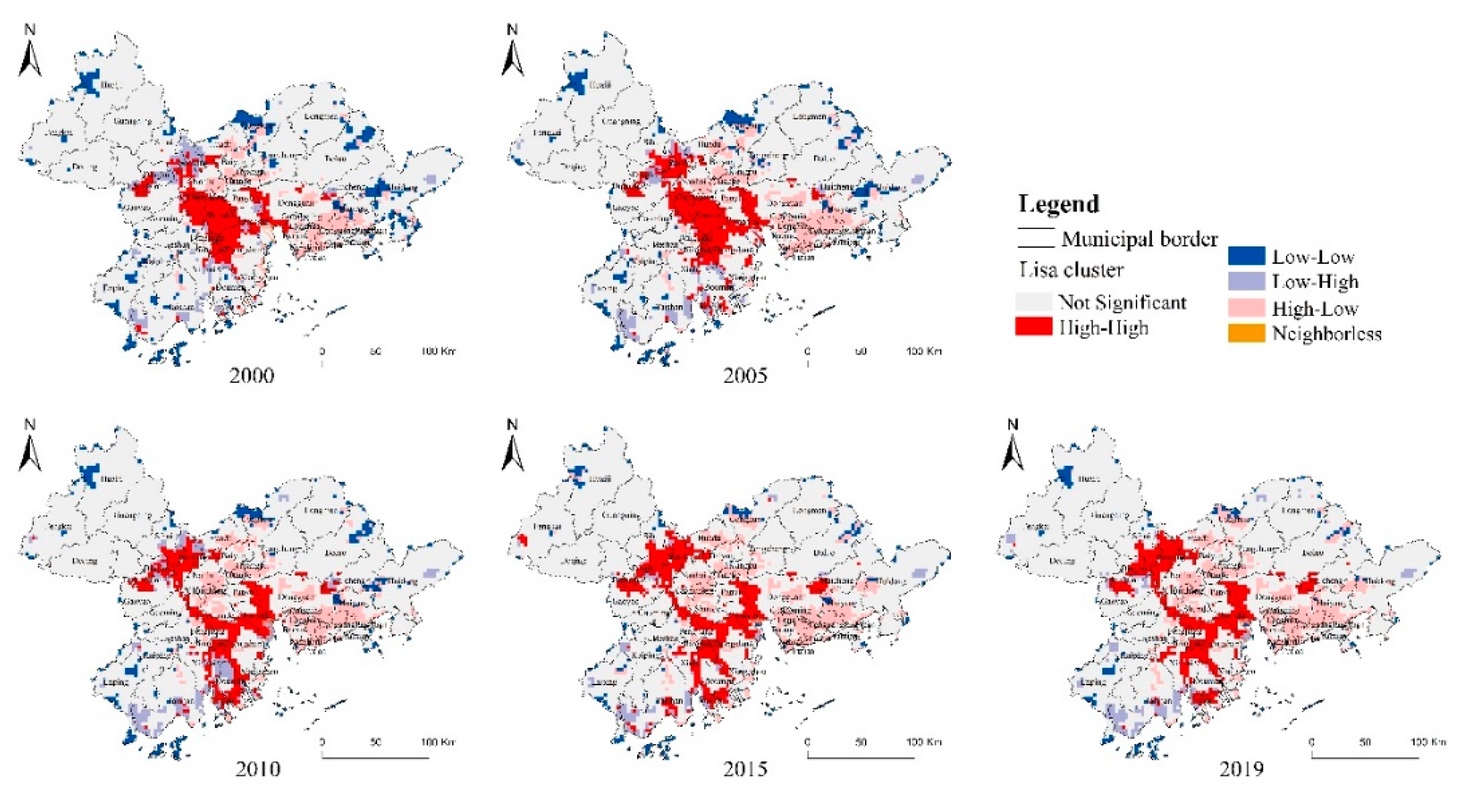
As seen in Table 7 and Figure 9: (1) the global Moran’s I index of comprehensive urbanization level and ecosystem service value in the PRD at raster scale was positive from 2000 to 2015, and the two were positively correlated. Places with high urbanization levels were more likely to gather high ecosystem service value, which changed to negative in 2019, and the two were negatively correlated, but their absolute values all converged to zero, indicating that the two spatially differ greatly and there is no significant spatial correlation. (2) From 2000 to 2005, the distribution of “high–high” agglomeration in the PRD was mainly concentrated in Foshan City, Duanzhou District in southeastern Zhaoqing City, Sanshui District and southeastern Sihui City, northwestern Zhongshan City, the junction of western Dongguan City with Panyu District and Nansha District, and the junction of northeastern Jiangmen City with Foshan City. Since 2010, Foshan City changed to “high–low” agglomeration and the “high–high” agglomeration area spread from Foshan City to Sanshui District, Dinghu District, Duanzhou District and the southeast of Sihui City in the southeast of Zhaoqing City, and to the middle of Nansha District, Dongguan City and the junction of Panyu District and Nansha District in the southeast of Dongguan City. and Nansha District, southward to the junction of Jiangmen City and Foshan City, Jianghai District, Jinwan District, central and northeastern Xinhui District, and western and northern Zhongshan City, the proportion of “high–high” clusters in the past 20 years showed a trend of first increasing and then decreasing, with an overall relative increase, and the spatial pattern gradually growing from a small ram’s horn layout to a large ram’s horn. (3) In the past 20 years, the spatial pattern of "low–low" agglomeration areas has changed less, mainly in the western part of Conghua District, Huizhou City, the northeastern part of Boluo County, the eastern and southern part of Huidong County, the western part of Huaiji County, Zhaoqing City, the northern and southern part of Enping City, Jiangmen. (4) The spatial pattern and numerical changes of the “low–high” agglomeration areas in the past 20 years are relatively small, mostly concentrated in Sanshui District, Dinghu District, Xinhui District, Doumen District, Jinwan District and other “high–high” agglomeration areas and the southern part of Taishan City and the eastern part of Huidong County. (5) From 2000 to 2005, the “high–low” agglomeration areas in the PRD were concentrated in Guangzhou, Shenzhen, central Dongguan and southwestern Conghua District, and from 2010, the “high–low” agglomeration areas added Foshan City on top of the previous ones, except for a slight expansion north of Shenzhen and a significant shift from the original "low–low" to “high–low” in northeastern Boluo County, and the proportion of agglomeration areas continued to increase in the past 20 years.

4. Discussion

4.1. Calculation of the Ecosystem Service Value in the PRD

In this paper, the ESV of the PRD urban agglomeration is assessed using a modified unit area value equivalent factor method based on correction coefficients, which is easy to operate compared to market value, shadow engineering and alternative cost methods, and is applicable to regional, national and global scales [38]. In recent years, more studies on the PRD have accounted for ESV with the help of this method; Xiao [39] assessed the ESV of the PRD from 2000 to 2015 with Guangzhou-Foshan-Zhaoqing as an example, which were 1402.68, 1440.98, 1413.88, and 139.909 billion yuan, showing a trend of first increasing and then decreasing year by year. The assessment results after area conversion are similar to ours and the change trend is consistent; Xu [40] assessed the ESV of the PRD urban agglomeration from 2000 to 2015 to be about 300 billion yuan, and the assessment results are also similar, so the conclusions of this study are reliable.

4.2. Calculation of Urbanization Level in the Pearl River Delta

There are many methods for calculating the urbanization level [18,32], and this paper draws on existing studies to characterize the comprehensive urbanization level of the region by selecting indicators from three aspects: population, life, and economy. On the one hand, the dimensions affected by the urbanization process are far richer than the urbanization level system constructed in this study, and it is more difficult to provide an integrated description of the urbanization level due to data limitations. On the other hand, no scholars have yet spatialized the comprehensive urbanization level using nighttime lighting data, and more scientific and accurate and realistic adjustments will be made in the future through relevant literature studies and parameter corrections.

4.3. Spatial–Temporal Evolution Patterns of Urbanization Level and ESV

By analyzing the spatial–temporal evolution of urbanization level and ESV in the PRD from 2000 to 2019, it is found that: high-value areas with comprehensive urbanization level are concentrated in the middle of the PDR, mainly in Guangzhou and Shenzhen, with a large expansion of high-value area starting in 2005 in particular. Guangzhou and Shenzhen, as the first cities to develop, have driven the development of the surrounding areas, and the urbanization spillover effect is obvious, showing a mature urbanization pattern in the region. The total value of ecosystem service shows a trend of first increasing and then decreasing, and the value added mainly comes from the ecological value contribution of water bodies, forest land and other land resources, while the decrease of ESV year by year after 2010 reflects the negative effect of urbanization changing land use cover has emerged, which means the expansion of building land has caused more serious damage to ecosystem service. ESV from the spatial distribution of high in the belly and low around the PRD in 2000 to low in Guangzhou, Shenzhen and Foshan and high in Foshan with northwest, southeast and south in 2019, with enhanced spatial heterogeneity and uneven distribution. Therefore, it is necessary not only to increase the overall efforts to protect natural resources in the future, but also to pay more attention to the spatial equalization of ecological service value, especially to adjust and optimize the proportion of land types in areas with high urbanization levels.

4.4. Spatial Relationship between Urbanization Level and ESV

The spatial interaction between urbanization level and ESV generally has a spillover effect, and a large number of studies have shown that they are negatively correlated [26,41], and by studying the spatial relationship between the comprehensive urbanization level and ESV in the PRD from 2000–2019, it was found that there is a negative correlation between the two at the county scale, and there is no significant spatial correlation at the raster scale, indicating that the spatial The spatial correlation between the two was found to be negative at the county scale, but not at the raster scale, indicating that the spatial correlation between the two was different at different scales, with obvious scale-dependent characteristics [37].At the spatial level, the raster scale shows obvious spatial heterogeneity compared with the county scale, and the “high–high” agglomeration was mostly concentrated in and around Foshan City from 2000 to 2005, but from 2010 onward, the region was influenced by the urbanization level of Guangzhou City and changed to “high–low” agglomeration, which was mainly distributed in "As one of the cities with the most drastic transformation in the past 20 years, Foshan City should focus on ecological environmental protection during its urbanization development, avoiding the negative impact of the spillover effects of arable land operation and urban construction and development on the natural ecology, and at the same time, it is necessary to set up as many eco-friendly land types in the natural areas at the edge of the city as possible [42], for instance add water body and wetland in the edge of Foshan City

5. Conclusions

This study measured the urbanization level and ecosystem service value of the PRD Urban Agglomeration from 2000–2019 from a dual-scale perspective, and analyzed their spatial–temporal evolution and spatial relationships, which are important for fine-grained analysis of the development of the region. The results of the study indicate that:
  • In the past 20 years, the overall trend of urbanization level and ecosystem service value in the PRD has been on the rise. Among them, the regional differences in urbanization level are significant, and the urbanization spillover effect in the central region drives the development of neighboring regions with centripetal nature; the spatial heterogeneity of ecosystem service value is strong, with the largest change between 2005 and 2010 and a gradual decline after 2010.
  • At the numerical level, both single and comprehensive urbanization are significantly correlated with ESV. ESV is negatively correlated with comprehensive, population, and economy urbanization levels, and positively correlated with life urbanization.
  • At the spatial level, comprehensive urbanization and ESV in the PRD from 2000 to 2019 are spatially negatively correlated at the county scale, while the spatial correlation is not significant at the raster scale. From 2000 to 2005, the distribution of “high–high” agglomeration is mainly concentrated in and around Foshan City; from 2010, the “high–low” agglomeration area expands from Tianhe District to Foshan City and occupies Foshan; from 2015 to 2019, the “high–high” and “high–low” agglomeration distribution is dominant.
  • Foshan City is the area that has changed most dramatically in the past 20 years, from a “high–high” agglomeration to a “high–low” agglomeration, and the rapid urbanization has damaged to Foshan’s waters and green areas. Tianhe, Yuexiu District in Guangzhou City and Nanshan District in Shenzhen City, have always maintained the “high–low” clustering, indicating that the construction land has encroached on the local natural land cover and the ecological resource environment is poor.
At the same time, there are shortcomings in this study. First, with the deepening of the concept of "new urbanization", the indicators used in this study cannot accurately reflect the new urbanization level of the region, and a more combined and complete measurement system is needed. Secondly, as the factors influencing urban agglomerations are too complex, covering population, economic and living conditions as well as ecology, smaller urban areas will be focused on for specific exploration. How to identify the key factors of smaller urban areas, reveal their development mechanisms and maintain a balanced ecosystem therefore proves to be necessary in the urbanization process.

Author Contributions

Conceptualization, Y.M. and L.H.; methodology, Y.M., L.H. and Z.Z.; software, Y.M. and L.H.; validation, Y.M. and L.H.; formal analysis, Y.M., L.H. and Z.Z.; investigation, Y.M. and L.H.; resources, Y.M. and Z.Z.; data curation, Y.M. and L.H.; writing—original draft preparation, Y.M. and L.H.; writing—review and editing, Y.M., L.H. and Z.Z.; visualization, Y.M.; supervision, Y.M., L.H. and Z.Z.; project administration, Y.M., L.H. and Z.Z. All authors have read and agreed to the published version of the manuscript.

Funding

This research received no external funding.

Institutional Review Board Statement

The study was conducted according to the guidelines of the Declaration of Helsinki, and approved by School of Geography, South China Normal University.

Informed Consent Statement

Informed consent was obtained from all subjects involved in the study.

Data Availability Statement

New data generated is shared through this article. All other sources of data are cited throughout the paper.

Acknowledgments

We would like to thank the editors and reviewers for their efficiency, constructive advice and appreciation of our paper.

Conflicts of Interest

The authors declare no conflict of interest.

References

  1. Liu, Y.; Yang, R. The spatial characteristics and formation mechanism of the county urbanization in China. Acta Geogr. Sin. 2012, 67, 1011–1020. [Google Scholar]
  2. Peng, J.; Wang, A.; Liu, Y.; Ma, J.; Liu, J. Research progress and prospect on measuring urban ecological land demand. Acta Geogr. Sin. 2015, 70, 333–346. [Google Scholar]
  3. Van, W.J.; Calow, P.; Dollacker, A.; Maltby, L.; Olander, L.; Tuvendal, M.; Van, H.G. Identifying and assessing the application of ecosystem services approaches in environmental policies and decision making. Integr. Environ. Assess. 2017, 13, 41–51. [Google Scholar]
  4. Faulkner, S. Urbanization impacts on the structure and function of forested wetlands. Urban. Ecosyst. 2004, 7, 89–106. [Google Scholar] [CrossRef]
  5. Kreuter, U.P.; Harris, H.G.; Matlock, M.D.; Lacey, R.E. Change in ecosystem service values in the San Antonio area, Texas. Ecol. Econ. 2001, 39, 333–346. [Google Scholar] [CrossRef]
  6. Ou, X.; Zhu, X.; He, Q. Incorporating ecosystem services with ecosystem health for ecological risk assessment: A case study in Changsha-Zhuzhou-Xiangtan urban agglomeration, China. Acta Ecol. Sin. 2020, 40, 5478–5489. [Google Scholar]
  7. Huang, Z.; Wang, F.; Cao, W. Dynamic analysis of an ecological security pattern relying on the relationship between ecosystem service supply and demand: A case study on the Xiamen-Zhangzhou-Quanzhou city cluster. Acta Ecol. Sin. 2018, 38, 4327–4340. [Google Scholar]
  8. Yang, Q.; Liu, G. Wetland ecosystem services assessment based on emergy: A case of Pearl River Delta Urban Agglomeration. Acta Sci. Circumst. 2018, 38, 4527–4538. [Google Scholar]
  9. Cao, J.; Zhang, Z.; Chen, S.; Yang, Y.; Kuang, T.; Chen, Y.; Li, Q.; Mao, Y.; Dong, J. The response of ecosystem services to landscape pattern changes in the Guangdong—Hong Kong—Macao Greater Bay Area from 1996 to 2015. J. South China Norm. Univ. (Nat. Sci.) 2020, 52, 93–105. [Google Scholar]
  10. Habitat, U.N.H. Urban Indications Guideliners; United Nations Publications: New York, NY, USA, 2004; pp. 8–9. [Google Scholar]
  11. Guo, Y.; Wei, H. A review of literature on urbanization quality evaluation. J. Grad. Sch. Chin Acad. Soc. Sci. 2013, 2, 37–43. [Google Scholar]
  12. Paul, J.C. An index of rurality for England and Wales. Reg. Stud. 1997, 11, 32–46. [Google Scholar]
  13. Zhang, T.; Liang, J.; Song, J. Summarization of studies on measuring of urbanization in China. Urban. Stud. 2002, 9, 36–41. [Google Scholar]
  14. Xue, D. The Urbanization Process of Loess Plateau and Its Ecological and Environmental Response. Ph.D. Thesis, Shanxi Normal University, Xi’an, Shanxi, China, 2019. [Google Scholar]
  15. Wang, F. Study on the quality measurement and coordinated development of population-land urbanization in Shandong Peninsula Urban Agglomeration. Sci. Geogr. Sin. 2020, 40, 1345–1354. [Google Scholar]
  16. Wang, S.; Wang, X.; Fan, D.; Song, Y.; Lin, H. Ecological effects assessment of urbanization in Jilin central urban agglomeration area. Human. Geogr. 2017, 32, 90–98. [Google Scholar]
  17. Jin, D.; Kong, X. Evaluation and Spatial Correlation Analysis of Urbanization Development Quality in Hubei Province. Resour. Environ. Yangtze Basin. 2020, 29, 2146–2155. [Google Scholar]
  18. Ma, H.; Sun, Z. Comprehensive urbanization level and its dynamic factors of five Central Asian countries. Acta Geogr. Sin. 2021, 76, 367–382. [Google Scholar]
  19. Lucas, R.E. Making a miracle. Econometrica 1993, 61, 251–272. [Google Scholar] [CrossRef]
  20. Ho, C.-Y.; Wang, W.; Yu, J. International knowledge spillover through trade: A time-varying spatial panel data approach. Econ. Lett. 2018, 162, 30–33. [Google Scholar] [CrossRef]
  21. Ambec, S.; Coria, J. Policy spillovers in the regulation of multiple pollutants. J. Environ. Econ Manag. 2018, 87, 114–134. [Google Scholar] [CrossRef]
  22. Zhang, J.; Lei, G.; Qi, L.; Ding, X.; Chen, C.; Liu, X. The landscape pattern and ecological service value in Danjiangkou City under land use change from 2003 to 2018. Acta Ecol. Sin. 2021, 41, 1280–1290. [Google Scholar]
  23. Wang, H.; Qin, F.; Zhu, J.; Zhang, C. The effects of land use structure and landscape pattern change on ecosystem service values. Acta Ecol. Sin. 2017, 37, 1286–1296. [Google Scholar]
  24. Shi, H.; Cheng, J.; Fei, L.; Cheng, J. LandUse Transition and changes of ecosystem service function in urban agglomerations of the Yangtze River Delta from 1990 to 2015. Res. Soil Water Conserv. 2019, 26, 301–307. [Google Scholar]
  25. Yao, X.; Zeng, J.; Li, W. Spatial correlation characteristics of urbanization and land ecosystem service value in Wuhan Urban Agglomeration. Trans. Chin. Soc. Agric. Eng. 2015, 31, 249–256. [Google Scholar]
  26. Chen, W.; Liu, Z.; Li, J.; Ran, D.; Zeng, J. Mapping the spatial relationship between ecosystem services and urbanization in the middle reaches of the Yangtze River Urban Agglomerations. Acta Ecol. Sin. 2020, 40, 5137–5150. [Google Scholar]
  27. Wang, D.; Sun, Z.; Sun, R.; Chen, J.; Zhang, W.; Zhang, X.; Wang, X. Spatial-temporal Dynamic Evolution of Ecosystem Service Value in Beijing-Tianjin-Hebei Urban Agglomeration. J. Ecol. Environ. 2019, 28, 1285–1296. [Google Scholar]
  28. Xie, G.; Zhang, C.; Zhang, L.; Chen, W.; Li, S. Improvement of the Evaluation Method for Ecosystem Service Value Based on Per Unit Area. J. Nat. Resour. 2015, 30, 1244–1255. [Google Scholar]
  29. Zhu, Y.; Yao, S. The coordinated development of environment and economy based on the change of ecosystem service value in Shaanxi province. Acta Ecol. Sin. 2021, 41, 3331–3342. [Google Scholar]
  30. Xu, L.; Xu, X.; Luo, T.; Zhu, G.; Ma, Z. Services based on landuse: A case study of Bohai Rim. Res. Geogr. 2012, 31, 1776–1785. [Google Scholar]
  31. Xie, G.; Xiao, Y.; Zhen, L.; Lu, C. Study on ecosystem services value of food production in China. Chin. J. Eco-Agric. 2005, 13, 10–13. [Google Scholar]
  32. Sun, X.; Zhang, Z. Coupling and coordination level of the population, land, economy, ecology and society in the process of urbanization: Measurement and spatial differentiation. Sustainability 2021, 13, 3171. [Google Scholar] [CrossRef]
  33. Zhou, Q.; Liu, D. Study on the coordinated development of urban resilience and urbanization level in the urban agglomeration of Yangtze River Delta. Res. Soil Water Conserv. 2020, 27, 286–292. [Google Scholar]
  34. Rao, Y.; Li, C.; Li, H. Urbanization-coordinated development level of natural ecology and its impact on urban-rural income gap: Based on the perspective of a comparative study of urban agglomerations in Chengdu-Chongqing, Central Guizhou and Central Yunnan. Ecol. Econ. 2020, 36, 77–83. [Google Scholar]
  35. Anselin, L. Local indicators of spatial association-LISA. Geogr. Anal. 1995, 27, 93–115. [Google Scholar] [CrossRef]
  36. Li, Z.; Zhang, J.; Geng, Y. Effects of ecological diffusions of cities around Yangtze River Economic Belt basing on spatial relation. J. China Agric. Univ. 2017, 22, 161–171. [Google Scholar]
  37. Lei, J.; Chen, Z.; Wu, T.; Li, Y.; Yang, Q.; Chen, X. Spatial autocorrelation pattern analysis of land use and the value of ecosystem services in northeast Hainan island. Acta Ecol. Sin. 2019, 39, 2366–2377. [Google Scholar]
  38. Wang, X.; Gao, Z.; Su, J.; Chen, Z.; Zheng, M.; Sun, Y.; Ji, D. Assessment methods of regional ecosystem service value and a case study of Dongjiang River basin. J. Environ. Engin. Tech. 2018, 8, 212–220. [Google Scholar]
  39. Xiao, H.; Li, H.; Wang, L.; Chen, J.; Han, Y. Changes of landuse and ecosystem service balue in Guangdong-Hongkong-Macau Greater Bay Area: A case study of Guangzhou-Foshan-Zhaoqing. Res. Soil Water Conserv. 2020, 27, 207–212. [Google Scholar]
  40. Xu, Z.; Zhou, Y.; He, Y.; Kuang, H.; He, D. Study on the prediction of ecological system service values based on the changes of land use in Guangdong-Hongkong-Macau Greater Bay Area. Ecol. Sci. 2020, 39, 207–212. [Google Scholar]
  41. Ou, X.; Zhu, X.; He, Q. Spatial interaction between urbanisation and ecosystem services: A case study in Changsha-Zhuzhou-Xiangtan urban agglomeration, China. Acta Ecol. Sin. 2019, 39, 7502–7513. [Google Scholar]
  42. Maiorano, L.; Falcucci, A.; Boitani, L. Size-dependent resistance of protected areas to land-use change. P. Roy. Soc. B Biol. Sci. 2008, 275, 1297–1304. [Google Scholar] [CrossRef] [PubMed] [Green Version]
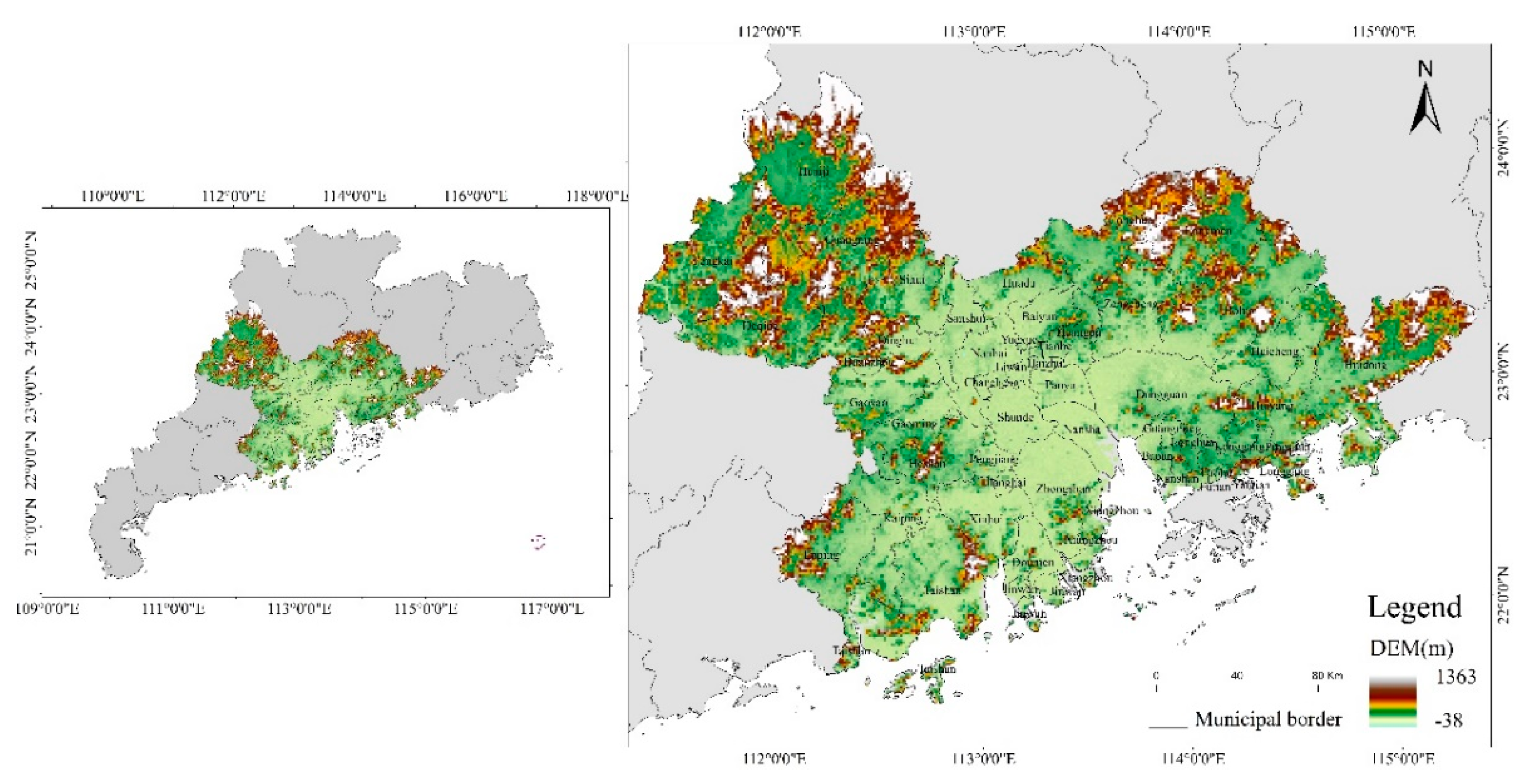
Figure 1. The location of the Pearl River Delta Urban Agglomeration.
Sustainability 13 08537 g001
Figure 2. Flowchart of spatial relationships between nighttime light and comprehensive urbanization level.
Sustainability 13 08537 g002
Figure 3. Spatial–temporal changes in the value of ecosystem service value in the Pearl River Delta at the county scale.
Sustainability 13 08537 g003
Figure 4. Spatial–temporal changes of ecosystem service value in the Pearl River Delta at the raster scale.
Sustainability 13 08537 g004
Figure 5. The urbanization level of Pearl River Delta Urban Agglomeration in 2000–2019.
Sustainability 13 08537 g005
Figure 6. Spatial–temporal changes of comprehensive urbanization level in the Pearl River Delta at county scale.
Sustainability 13 08537 g006
Figure 7. Spatial–temporal changes of comprehensive urbanization level in the PRD at raster scale.
Sustainability 13 08537 g007
Figure 8. Clustering change of comprehensive urbanization level and ESV in the Pearl River Delta at county scale.
Sustainability 13 08537 g008
Figure 9. Clustering change of comprehensive urbanization level and ESV in the Pearl River Delta at raster scale.
Sustainability 13 08537 g009
Table 1. Ecosystem service value coefficient per unit area of different land use types in the Pearl River Delta/(yuan/hm2 *a).
YearCroplandWoodlandGrasslandWater BodyWetlandConstruction LandUnused Land
20007472.8335,213.1029,437.27237,635.9598,414.310.001229.71
20058007.8437,734.1531,544.80254,649.24105,460.180.001317.75
201010,951.2851,604.0943,139.72348,250.66144,224.180.001802.11
201511,271.5153,113.0444,401.17358,433.86148,441.440.001854.80
201910,952.3451,609.0843,143.90348,284.36144,238.140.001802.28
Table 2. Urbanization evaluation index system of Pearl River Delta Urban Agglomeration.
TargetGuideline IndicatorIndicator PropertiesWeights
Urbanization LevelLife UrbanizationNumber of beds per 1000 people [32]+ 10.06
Energy consumption per unit of GDP [17]20.08
Number of students enrolled in general secondary schools per 1000 population [15]+0.06
Economy UrbanizationGDP per capita [18]+0.11
Percentage of value of secondary and tertiary industries [16]+0.01
Total retail sales of social consumer goods [33]+0.32
Population UrbanizationPercentage of urban population [34]+0.11
Population density [26]+0.24
1, 2 “+” represents a positive indicator and “−” a negative indicator.
Table 3. Combination of weights for different lighting indices.
Weighted Combinations
(u,v)
R2Weighted Combinations
(u,v)
R2
(0.1,0.9)0.55(0.6,0.4)0.67
(0.2,0.8)0.57(0.7,0.3)0.70
(0.3,0.7)0.60(0.8,0.2)0.74
(0.4,0.6)0.62(0.9,0.1)0.81
(0.5,0.5)0.64(1,0)0.79
Note: All passed the significance test at the 0.01 level.
Table 4. ESV and rate of change in the Pearl River Delta at the county scale in 2000–2019.
CountyESV (108 Yuan) and Its Change Rate (%) in 2000–2019
200000–05200505–10201010–15201515–19201900–19
Baiyun30.550.7930.7941.4443.544.0245.30−4.7143.1641.31
Baoan27.34−30.8918.9024.3323.49−14.9019.99−7.1818.56−32.12
Boluo112.998.20122.2538.76169.641.85172.78−3.13167.3748.13
Chancheng24.34−11.0321.66−50.4910.72−2.3610.47−2.5210.21−58.07
Conghua66.357.5171.3339.1399.231.44100.66−2.6498.0047.71
Deqing83.826.0988.9336.67121.542.70124.82−2.96121.1344.51
Dinghu43.8925.4455.0664.1090.350.7591.03−4.4686.9798.14
Dongguan132.45−5.37125.3442.25178.30−1.04176.46−4.50168.5127.22
Doumen36.1048.5453.62140.60129.02−42.9073.67−3.9170.7996.10
Duanzhou21.68−26.3015.9833.7321.373.1622.05−8.2120.24−6.67
Enping67.268.3572.8838.06100.611.19101.81−1.49100.3049.12
Panyu47.603.9249.4732.0465.31−2.0663.97−3.1961.9330.11
Fengkai108.677.27116.5735.59158.052.78162.45−3.04157.5044.93
Futian2.04−0.722.0389.573.840.223.85−4.433.6880.26
Gaoming54.665.6757.7629.1774.612.1176.18−3.0773.8435.09
Gaoyao109.507.99118.2542.22168.183.01173.24−3.52167.1552.65
Guangming7.85−13.576.7923.538.38−2.258.197.438.8012.11
Guangning95.347.76102.7436.68140.422.39143.77−2.85139.6846.50
Haizhu8.17−0.958.1039.8511.322.9711.66−3.1111.3038.20
Heshan58.533.8460.7727.7877.661.0078.44−3.3075.8429.59
Huadu46.170.3746.3437.9363.912.2365.34−2.6363.6237.80
Huaiji128.716.96137.6737.22188.912.23193.13−2.90187.5445.70
Huangpu26.670.1926.7233.8035.750.4435.91−5.0334.1027.87
Huicheng76.796.0281.4139.19113.312.30115.91−5.36109.7042.86
Huidong115.6410.99128.3536.46175.161.64178.03−3.07172.5649.22
Huiyang39.323.4840.6931.7153.602.1754.76−5.9451.5130.98
Jianghai19.13−1.2918.884.9719.825.4720.90−4.2520.014.64
Jinwan26.1155.1140.5056.3363.31−4.7660.29−10.4853.97106.73
Kaiping72.787.1577.9839.04108.431.15109.67−2.69106.7246.64
Liwan3.447.433.7035.905.0316.055.84−3.055.6664.26
Longgang24.542.2125.0836.3334.190.8134.47−2.5933.5836.83
Longhua6.26−6.525.8628.777.54−4.417.21−11.246.402.14
Longmen85.795.9890.9236.58124.172.67127.48−2.96123.7144.20
Luohu3.737.484.0143.065.732.265.86−2.745.7052.92
Nanhai109.16−1.07108.00−16.0890.63−5.3485.79−3.1483.09−23.88
Nansha59.6215.3568.7742.0897.71−7.8490.05−1.8988.3548.18
Nanshan5.59−3.705.3823.756.665.597.03−1.576.9223.85
Pengjiang34.632.0935.353.7136.661.2637.12−3.2935.903.68
Pingshan8.96−2.568.7323.2710.76−3.1110.42−2.7610.1413.18
Sanshui82.905.9087.7936.48119.821.14121.19−3.54116.9041.01
Shunde149.99−8.99136.51−50.3967.73−0.6167.32−3.6164.89−56.74
Sihui70.8314.2280.9146.85118.812.29121.54−4.80115.7063.34
Taishan154.7914.20176.7640.05247.552.58253.93−2.71247.0559.61
Tianhe6.710.766.7633.129.002.359.22−3.028.9433.14
Xiangzhou20.4619.9624.5436.0133.38−25.5124.87−5.3123.5415.07
Xinhui94.158.09101.7748.59151.22−7.85139.35−4.28133.3841.66
Yantian4.450.844.4934.776.050.526.08−2.725.9132.90
Yuexiu1.2136.911.6545.332.403.022.47−2.902.4099.04
Zengcheng62.854.7865.8637.6890.672.9593.35−3.4790.1143.37
Zhongshan149.99−3.35144.9626.14182.84−7.99168.24−3.25162.788.53
All2830.505.482985.5132.853966.35−1.333913.55−3.523775.7333.39
Table 5. Pearson relating analysis between urbanization level and ESV.
Compr_urPop_urEco_urLife_ur
ESV−0.439 ***−0.539 ***−0.281 ***0.326 ***
*** indicates significant correlation at the 0.01 level.
Table 6. Global Moran’s I index in the Pearl River Delta at county scale in 2000–2019.
Year20002005201020152019
Global Moran’s I−0.459−0.447−0.479−0.435−0.467
Table 7. Percentage of each cluster in the Pearl River Delta in 2000–2019.
YearPercentage of Each Cluster/%Global Moran’s I
Not SignificantHigh–HighLow–LowLow–HighHigh–LowNeighborless
200075.626.757.963.815.680.170.195
200574.577.896.453.577.290.230.123
201074.077.635.564.358.150.240.051
201574.639.043.962.639.510.230.037
201974.628.463.893.199.580.26−0.009
Publisher’s Note: MDPI stays neutral with regard to jurisdictional claims in published maps and institutional affiliations.