Forecasting Carbon Price with Secondary Decomposition Algorithm and Optimized Extreme Learning Machine

Abstract

Carbon trading is a significant mechanism created to control carbon emissions, and the increasing enthusiasm for participation in the carbon trading market has forced the emergence of higher-precision carbon price prediction models. Facing the complexity of carbon price time series, this paper proposes a carbon price forecasting hybrid model based on secondary decomposition and an improved extreme learning machine (ELM). First, the complementary ensemble empirical mode decomposition with adaptive noise (CEEMDAN) is utilized to decompose the carbon price several intrinsic modal functions to initially weaken the non-linearity of the original carbon price data. Secondly, the first intrinsic mode function (IMF1) with the strongest volatility is processed by the variational mode decomposition (VMD). Then, the partial autocorrelation function (PACF) is applied to obtain the model input variables for subsequences. Finally, the ELM improved by the bald eagle search (BES) algorithm is utilized to make predictions. In the empirical analysis, five actual datasets from three carbon markets are used to verify the prediction performance of the proposed model. Based on the six evaluation indicators of the predicted results, the proposed model is the best performer among all models, which suggests that CEEMDAN-VMD-BES-ELM is effective and stable in predicting carbon price.

1. Introduction

From a global perspective, the industrial revolution has promoted the development and progress of human society. However, the greenhouse gases emitted by the massive burning of fossil fuels are also irreversible to the environment [1]. Existing research shows that in recent years, the degree of temperature rise has become more intense, and the frequency of natural disasters has become more frequent [2]. The impact of global warming is reflected in all aspects, such as the marine ecological crisis [3], the decline in crop yields [4], the abnormal water cycle [5], and the changes in regional biological communities [6], which have brought huge challenges to human survival. Therefore, it is necessary to curb the tension of global warming and control the emission of greenhouse gases.

The international community and government agencies have made continuous exploration and made tremendous efforts. Currently, by putting carbon emission rights on the shelves as a commodity, and using market economy means to promote carbon pricing, thereby restricting the behavior of market participants is an effective means to control carbon emissions [7,8]. As the forerunner of this policy, the European Union established the European Union Emissions Trading System (EU ETS) in 2005, which has been proven to effectively reduce energy consumption and control carbon emissions [9]. The Chinese government has also actively responded to the call of the international community. Since 2011, it has established carbon trading pilots in eight provinces and cities including Hubei, Guangdong, and Shenzhen, and it is committed to energy conservation and emission reduction [10]. At the National People’s Congress and the Chinese Political Consultative Conference (NPC and CPPCC) in 2021, the Chinese government for the first time included “carbon neutrality” and “carbon peaking” in the government work report, which shows its firm faith in sustainable development. Simultaneously, as the world’s largest developing country, China’s national carbon market officially opened in June 2021, which will surely inject new vitality into the construction of the world carbon market.

In the carbon trading market, the change of supply and demand directly affects the price of carbon emission rights, regulating the allocation of market resources and the production and operation activities of related enterprises [11]. Hence, the accuracy of carbon price forecast is crucial for maintaining the stability of the carbon market, for policymakers to establish reasonable mechanisms, and for market participants to make prompt and effective decisions [12]. In addition, the carbon trading market is a policy market with strong government intervention, and the changes of internal policies and external environment lead to the non-linearity and non-stationarity of carbon price [13]. Therefore, the prediction of carbon price is quite challenging, and a large number of scholars are constantly experimenting with it. The main methods could be summarized as traditional statistical models and artificial intelligence models, as well as hybrid forecasting models combined with them. Benz and Truck [14] faced the complexity of the carbon price and performed the autoregressive generalized autoregressive conditional heteroscedasticity (AR-GARCH) to predict the carbon spot price. Facing the over-fitting problem in carbon price forecasting, Koop and Tole [15] utilized dynamic model averaging (DMA) to successfully forecast the carbon price.

In recent years, artificial intelligence models have been favored by scholars because of their powerful generalization capabilities. Fan et al. [16] noticed the chaotic nature of carbon prices and employed artificial neural network (ANN) predictions combined with multi-layer perceptrons to predict carbon price. Zhu et al. [17] developed a least squares support vector regression (LSSVR) carbon price prediction model. Han et al. [18] constructed a carbon price prediction model based on the back-propagation neural network (BPNN) and achieved high prediction accuracy. Zhu and Wei [19] established a carbon price prediction model based on the least squares support vector machine (LSSVM), which performed best in empirical analysis. However, the chaotic nature of the carbon price may lead to the prediction accuracy of the individual model being unsatisfactory [20]. Data preprocessing technology can eliminate or reduce the complexity of data and extract effective features. Therefore, the hybrid model combined with the decomposition algorithm has spread in the field of carbon price forecasting and has gradually become the mainstream method.

Chevallier [21] applied wavelet transform (WT) to the exploration of carbon prices and achieved high prediction accuracy. Zhu [22] utilized empirical mode decomposition (EMD) to process carbon prices in the constructed hybrid model. Zhou et al. [23] combined ensemble empirical decomposition (EEMD) and multiple prediction models to separately predict the obtained different frequency sub-sequences. Zhu et al. [24] proposed a carbon price combination forecasting method based on variational modal decomposition (VMD), which showed superior forecasting performance in all cases. However, further studies have shown that for time series forecasting, reprocessing of the high-frequency series obtained by decomposing the original data through EMD, EEMD, CEEMDAN, etc., could break through the original accuracy limitations [25,26,27]. However, the current two-stage decomposition research in carbon price forecasting is not sufficient, and its applicability and rationality need to be further explored [28].

Taking full account of the chaotic characteristics of carbon price data, a novel hybrid prediction model based on complementary ensemble empirical mode decomposition with adaptive noise (CEEMDAN), variational mode decomposition (VMD), bald eagle search (BES) algorithm, and extreme learning machine (ELM) is proposed. Taking five datasets from three typical carbon markets in China as an example, six evaluation indicators are selected to verify the effectiveness of the model. The innovations and possible contributions of this article could be summarized as follows:

• A novel hybrid model for carbon price prediction is constructed, which combines CEEMDAN, VMD, BES, and ELM, providing a new path for accurate forecasting.
• The secondary decomposition algorithm CEEMDAN-VMD was applied to deal with carbon prices and explore its applicability in this field for the first time. The CEEMDAN and VMD are combined to remove the noise component in the carbon price series, reduce the irregularity of the data, and make the prediction easier.
• The excellent global search ability of BES is applied to optimize the weight and bias of ELM, overcomes its inherent instability, and further improve its generalization ability.
• In the empirical study, five sets of actual data from the Hubei, Guangdong, and Shenzhen carbon markets with large market transactions are used as cases. Meanwhile, through the construction of benchmark models and six evaluation indicators, the outstanding predictive performance and universality of CEEMDAN-VMD-BES-ELM are verified.

The rest of the paper is organized as follows: The main theoretical methods and the proposed hybrid model are explained in Section 2. Section 3 introduces data processing and model evaluation indicators. Section 4 contains the selection of input variables and empirical research. Finally, the conclusions and discussion of the article are presented in Section 5.

2. Methodologies

2.1. Complementary Ensemble Empirical Mode Decomposition with Adaptive Noise (CEEMDAN)

In the field of time-series forecasting, as an adaptive signal processing method, EMD can decompose complex data signals into a more stable finite number of intrinsic mode functions (IMFs), which is more suitable for forecasting [29]. However, modal aliasing during the EMD decomposition process may lead to the appearance of error components. Wu and Huang [30] further introduced Gaussian white noise to assist the decomposition and proposed ensemble EMD (EEMD). Meanwhile, reconstruction errors caused by white noise inevitably appear. Therefore, the complementary ensemble empirical mode decomposition with adaptive noise (CEEMDAN) was developed [31], and compared with EMD and EEMD, it has the advantages of good data separation effect and small calculation amount. In view of this, this article will use CCEMDAN to pre-treat the carbon price in order to obtain more effective decomposition components. The main process is as follows:

1. Construct the added noise sequence:

$$R_k\left(t\right)=R_1\left(t\right)+p_0·{\omega }_k\left(t\right).$$

(1)

Among them, $R_1\left(t\right)$ represents the original signal, ${\omega }_k\left(t\right)\left(k=1,2,\cdots ,N\right)$ is Gaussian white noise, and $p_0$ denotes the noise figure.

2. Reuse the EMD algorithm to decompose $R_k\left(t\right)$, and calculate the first modal component and residual signal of the noise sequence as follows:

$$\overline{IM{F}_1^k\left(t\right)}=\frac{1}{k}{{\displaystyle \sum }}_{k=1}^{N}IM{F}_1^k\left(t\right)$$

(2)

$$r_1\left(t\right)=f\left(t\right)-\overline{IM{F}_1^k\left(t\right)}.$$

(3)

3. Using the first residual signal $r_1\left(t\right)$ and adding the corresponding noise sequence $r_1\left(t\right)+p_1{E}_1[{\omega }_k\left(t\right)]$, the second mode is obtained:

$$\overline{IM{F}_2^k\left(t\right)}=\frac{1}{k}{\sum }_{k=1}^N{E}_1(r_1\left(t\right)+p_1{E}_1[{\omega }_k\left(t\right)]).$$

(4)

4. Repeat operations until the decomposition ends when the residuals are not suitable for decomposition.

2.2. Variational Mode Decomposition (VMD)

The variational mode decomposition (VMD) is a non-recursive decomposition method, which aims to decompose the signal into some quasi-orthogonal intrinsic modes with limited bandwidth [32]. In the processing of some complex signals, it shows better performance and robustness than some existing mode decompositions. Therefore, this paper utilizes VMD to decompose the more volatile IMF1 again to get a more stable sub-sequence, which makes the prediction more accurate. For a dimensional signal $f\left(t\right)$, the detailed process of VMD is summarized as below.

Step 1: Define the initial mode $u_k^1$, center pulsation $w_k^1$, and the Lagrangian multipliers ${\lambda }^1, k=1,2,\dots ,K,$ where $K$ is the total number of decomposition level and $u_k$ is the $k$th component of $f\left(t\right)$.

Step 2: Update the parameters $u_k$ and $w_k$ with

$$u_k^{n+1}=\frac{f\left(\omega \right)-{\sum }_{i\ne k}{u}_i\left(\omega \right)+\lambda \left(\omega \right)/2}{1+2\alpha {(\omega -{\omega }_k)}^2}$$

(5)

$$w_k^{n+1}=\frac{{\int }_0^{\infty }w{\left|u_k^{n+1}\left(\omega \right)\right|}^{2}dw}{{\int }_0^{\infty }{\left|u_k^{n+1}\left(\omega \right)\right|}^{2}dw}$$

(6)

where n presents the number of iterations, $f\left(\omega \right)$,$u_i\left(\omega \right)$, $\lambda \left(\omega \right)$, and $u_k^{n+1}\left(\omega \right)$ are the Fourier transform of $f\left(t\right)$, $u_i\left(t\right)$, $\lambda \left(t\right)$, and $u_k^{n+1}\left(t\right)$.

Step 3: Update the parameter $\lambda$.

Step 4: If it satisfies $\sum _k\left|\right|u_k^{n+1}-u_k^{n+1}|{|}_2^2/|\left|u_k^{n+1}\right|{|}_2^2<e$, the VMD algorithm is over; otherwise, return to Step 2.

2.3. Bald Eagle Search (BES) Algorithm

Inspired by the search strategy of bald eagles when hunting fish, a new meta-heuristic optimization algorithm—bald eagle search (BES)—was developed by Alsattar et al. [33]. In comparison with the traditional differential evolution (DE) algorithm, particle swarm optimization (PSO), and gray wolf optimization (GWO) algorithm, it shows stronger optimization capabilities and faster convergence speed [33]. Here, this paper will apply the excellent global search capabilities of BES to optimize the weights and thresholds of ELM to improve its generalization ability. The simulation process of BES is mainly divided into the following three stages.

Stage 1: Search space selection. When searching for prey, the bald eagle will choose a better foraging area based on the quantity. The position of the bald eagle update is determined by:

$$P_{i,new}=P_{best}+\alpha \ast r\left(P_{mean}-P_i\right)$$

(7)

where $i$ is the $i$th bald eagle individual, $\alpha$ represents the position change parameter, which is usually distributed between 1.5 and 2; $r$ is a random number distributed at $\left(0, 1\right)$; $P_{best}$ means the optimal position at the current stage; $P_{mean}$ denotes the average distribution position of the bald eagle after the end of this stage, and $P_i$ is the position of the $i$th bald eagle.

Stage 2: Prey search. The bald eagle searches for prey in a spiral flight in the selected search area. At this stage, the spiral flight attitude is expressed as below:

$$xr\left(i\right)=r\left(i\right) \ast sin\left(\theta \left(i\right)\right), yr\left(i\right)=r\left(i\right) \ast cos\left(\theta \left(i\right)\right)$$

(8)

$$x\left(i\right)=xr\left(i\right)/max\left(\left|xr\right|\right), y\left(i\right)=yr\left(i\right)/max\left(\left|yr\right|\right).$$

(9)

The polar angle and polar diameter of the equation are expressed as $\theta \left(i\right)$ and r(i) respectively; $x\left(i\right)$ and $y\left(i\right)$denote the position of the bald eagle, the value range is [–1, 1]. The updated position of the bald eagle is determined by:

$$P_{i,new}=P_{i }+x\left(i\right)· \left(P_i-P_{mean}\right)+y\left(i\right) · \left(P_{i }-P_{i+1 }\right).$$

(10)

Stage 3: Dive and capture of prey. The bald eagle quickly dives from the best position found to the prey, and other individuals in the population also move toward the best position and start hunting. The state during the dive is generated by:

$$P_{i,new}=rand \ast P_{best}+x\left(1\right)· \left(P_i-c1\ast P_{mean}\right)+y\left(1\right)· \left(P_i-c2\ast P_{mean}\right)$$

(11)

where the range of the random parameters $c1$ and $c2$ is [1, 2].

2.4. Extreme Learning Machine (ELM)

The gradient descent strategy used in the training of traditional neural networks may cause defects such as slow convergence, the disappearance of gradients, and sensitivity to parameter settings. The unique design structure of ELM gives it the advantages of fast convergence, fewer parameters to be adjusted, and strong generalization ability, which makes it widely used in research in various fields [34].

Suppose a set of data with $N$ samples, and the observation values are $y_t, t=1,2,\cdots ,N$. The number of ELM hidden layer nodes is $D$, and its output function could be expressed as:

$$f\left(x\right)={\displaystyle \sum }_{\begin{array}{c}j=1\\ \end{array}}^D{\beta }_j·g\left(w_j,b_j,x\right)=o_t, t=1,2,\cdots ,N$$

(12)

where ${\beta }_j$ represents the weight between the $j$th hidden unit and the output layer, $g\left(w_j,b_j,x\right)$ is the activation function, and $w_j$ and $b_j$ are the weight and bias of the $j$th layer, respectively. The goal of the ELM calculation process is to find suitable ${\beta }_j$, $w_j$, and $b_j$ values such that $\sum _{j=1}^D\left|o_t-y_t\right|=0$. However, the randomly generated weights and thresholds of ELM will affect its approximation ability, which will eventually lead to the instability of the final prediction effect of the model. This article will utilize BES to optimize its parameters and enhance its stability and performance.

2.5. The Proposed Model

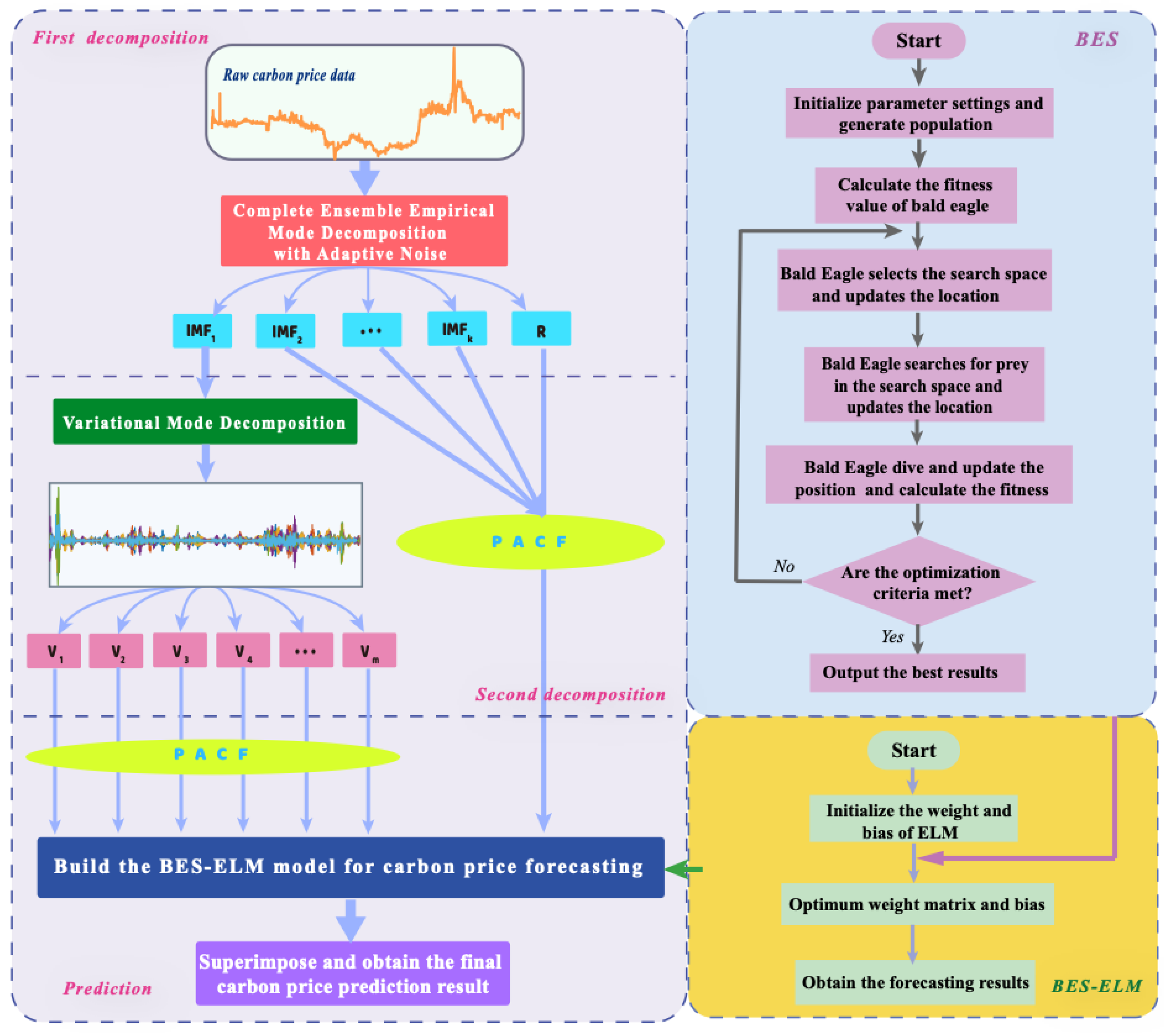
The framework of the CEEMDAN-VMD-BES-ELM is illustrated in Figure 1. The specific content is described as below.

(1)

The original carbon price data will be adaptively decomposed by CEEMDAN into k intrinsic mode functions (IMFs) and a residual component R. Among them, the first modal function is called IMF1. Obviously, the non-linear and non-stationary characteristics of the original data are weakened, which reduces the difficulty of prediction.

(2)

Among the many component sequences, IMF1 is the most irregular, which will directly affect the accuracy of carbon price prediction. Hence, in the second decomposition, IMF1 is further processed by VMD to obtain a more stable and ordered subsequence cluster ($V_m$).

(3)

The partial autocorrelation function is applied to analyze the inherent correlation of data information and determines the optimal input variables of the prediction model.

(4)

The ELM carbon price prediction model improved by the BES algorithm is constructed to predict all components. The outstanding global search capability of BES could determine the optimal weights and thresholds combination of ELM to achieve the goal of improving prediction accuracy.

(5)

The final carbon price prediction result will be obtained by summing the forecasting results of all subsequences.

3. Data Preprocessing

3.1. Data Description

Since 2011, China has successively established carbon trading pilots in eight provinces and cities. As of 31 December 2020, the total amount of carbon trading in each pilot is shown in Figure 2.

Among them, the transaction volume of the three carbon pilot projects in Hubei, Guangdong, and Shenzhen accounted for 75.9% of the total market, and they are more representative of the overall characteristics of China’s carbon market. Therefore, in this paper, their data from the opening of the market to 31 December 2020 are selected for empirical analysis. For the Shenzhen carbon market, this paper selects three-stage datasets with a longer time span including SZA-2013, SZA-2014, and SZA-2015.

Table 1. Description of the datasets.

Datasets	Type	Date (Day/Month/Year)	Size	Train	Test
Hubei	HBEA	2 April 2014–31 December 2020	1804	1487	317
Guangdong	GDEA	19 December 2013–31 December 2020	1918	1587	331
Shenzhen	SZA-2013	19 June 2013–31 December 2020	2102	1707	395
	SZA-2014	6 August 2014–31 December 2020	1682	1367	315
	SZA-2015	14 July 2015–31 December 2020	1345	1087	258

displays the basic information of the five datasets, which could be obtained from the Chinese carbon trading website (http://www.tanjiaoyi.com (accessed on: 20 January 2021)). The model training set and the testing set are divided into 4:1; that is, the first 80% of the samples are utilized to train the model, and the last 20% of the samples are used to evaluate the accuracy of the model. In addition, (a) and (b) in Figure 3 respectively describe the trend of the original data and the corresponding PACF results, which intuitively reflect the complex and non-stationary characteristics of carbon prices.

3.2. First Decomposition

Taking into account the inherent chaotic characteristics of the carbon price time series, the direct prediction effect is often unsatisfactory. The preprocessing of the original data could accurately extract the characteristics of the data and improve the prediction accuracy of the model. Take the actual data of Hubei carbon market as an example to illustrate the process of data processing in this article.

For the purpose of reducing the complexity of carbon price, the CEEMDAN is applied to process data and a series of component sequences are obtained. The results of the first decomposition of the Hubei carbon market and the PACF results of the corresponding sequence are presented in Figure 4. As shown in the figure, the original data are adaptively decomposed into 10 intrinsic modal functions and a residual sequence. Compared with the original sequence, each component sequence becomes more stable and regular, which significantly reduces the difficulty of forecasting.

3.3. Secondary Decomposition

To further break through the limitation of prediction accuracy, VMD is employed to reprocess the IMF1 obtained in the first decomposition. As shown in Figure 5a, IMF1 is decomposed into five more refined sub-sequences for prediction. Figure 5b is the result of PACF processing of the corresponding sequence, and the input variables of the model are determined according to the coefficients.

3.4. Input Selection

The carbon price time series is chaotic and can be regarded as a random process. The PACF is a method of describing stochastic processes, and the optimal input variables could be selected by analyzing the coefficient model [35]. In this paper,

Table 2. Input variables of forecasting models.

	Series	Lag
		HBEA	GDEA
First Decomposition	Raw data	$x_{t-1},x_{t-2},x_{t-5},x_{t-7}$	$x_{t-1}$
	IMF1	$x_{t-1},x_{t-2},x_{t-4},x_{t-5},x_{t-6},x_{t-7}$	$x_{t-1},x_{t-2},x_{t-3},x_{t-4},x_{t-7}$
	IMF2	$x_{t-1},x_{t-2},x_{t-3},x_{t-4},x_{t-6},x_{t-7}$	$x_{t-1},x_{t-2},x_{t-3},x_{t-4},x_{t-5},x_{t-6},x_{t-7}$
	IMF3	$x_{t-1},x_{t-2},x_{t-3},x_{t-4},x_{t-5},x_{t-6}$	$x_{t-1},x_{t-2},x_{t-3},x_{t-4},x_{t-6},x_{t-7}$
	IMF4	$x_{t-1},x_{t-2},x_{t-3},x_{t-4},x_{t-5},x_{t-6},x_{t-7}$	$x_{t-1},x_{t-2},x_{t-3},x_{t-4},x_{t-5},x_{t-6}$
	IMF5	$x_{t-1},x_{t-2},x_{t-3},x_{t-5},x_{t-6},x_{t-7}$	$x_{t-1},x_{t-2},x_{t-3},x_{t-4},x_{t-5},x_{t-7}$
	IMF6	$x_{t-1},x_{t-2},x_{t-3},x_{t-5},x_{t-6},x_{t-7}$	$x_{t-1},x_{t-2},x_{t-3},x_{t-4},x_{t-5},x_{t-6},x_{t-7}$
	IMF7	$x_{t-1},x_{t-2},x_{t-3},x_{t-4},x_{t-5},x_{t-6},x_{t-7}$	$x_{t-1},x_{t-2},x_{t-3},x_{t-4},x_{t-5},x_{t-6},x_{t-7}$
	IMF8	$x_{t-1},x_{t-2},x_{t-3},x_{t-4},x_{t-5},x_{t-6},x_{t-7}$	$x_{t-1}$
	IMF9	$x_{t-1}$	$x_{t-1}$
	IMF10	$x_{t-1}$
	Residual	$x_{t-1}$	$x_{t-1}$
Second Decomposition	$V_1$	$x_{t-1},x_{t-2},x_{t-3},x_{t-4},x_{t-5},x_{t-6},x_{t-7}$	$x_{t-1},x_{t-2},x_{t-3},x_{t-5},x_{t-6}$
	$V_2$	$x_{t-1},x_{t-2},x_{t-3},x_{t-4},x_{t-5},x_{t-6},x_{t-7}$	$x_{t-1},x_{t-2},x_{t-3},x_{t-4},x_{t-5},x_{t-6}$
	$V_3$	$x_{t-1},x_{t-2},x_{t-3},x_{t-4},x_{t-5},x_{t-7}$	$x_{t-1},x_{t-2},x_{t-3},x_{t-4},x_{t-5},x_{t-6}$
	$V_4$	$x_{t-1},x_{t-2},x_{t-4},x_{t-5},x_{t-6}$	$x_{t-1},x_{t-2},x_{t-3},x_{t-4},x_{t-6},x_{t-7}$
	$V_5$	$x_{t-1},x_{t-2},x_{t-3},x_{t-4},x_{t-5},x_{t-6}$	$x_{t-1},x_{t-2},x_{t-3},x_{t-4},x_{t-5},x_{t-6}$
	$V_6$	$x_{t-1},x_{t-2},x_{t-3},x_{t-4},x_{t-5},x_{t-6}$	$x_{t-1},x_{t-2},x_{t-3},x_{t-5},x_{t-6},x_{t-7}$

illustrates the results of selecting input variables for each sub-sequence of the Hubei and Guangdong carbon market data. Similarly, the PACF results of the three datasets of the Shenzhen carbon market are shown in

Table A1. Model input variables in Shenzhen market.

	Series	Lag
		SZA-2013	SZA-2014	SZA-2015
First Decomposition	Raw data	$x_{t-1},x_{t-2}$	$x_{t-1},x_{t-2},x_{t-7}$	$x_{t-1},x_{t-2}$
	IMF1	$x_{t-1}-x_{t-7}$	$x_{t-1}-x_{t-4},x_{t-6},x_{t-7}$	$x_{t-1},x_{t-2},x_{t-4}-x_{t-7}$
	IMF2	$x_{t-1}-x_{t-6}$	$x_{t-1}-x_{t-4},x_{t-6}$	$x_{t-1}-x_{t-4},x_{t-7}$
	IMF3	$x_{t-1}-x_{t-4},x_{t-7}$	$x_{t-1}-x_{t-6}$	$x_{t-1}-x_{t-6}$
	IMF4	$x_{t-1}-x_{t-7}$	$x_{t-1}-x_{t-4},x_{t-6},x_{t-7}$	$x_{t-1}-x_{t-7}$
	IMF5	$x_{t-1}-x_{t-7}$	$x_{t-1}-x_{t-3},x_{t-5}-x_{t-7}$	$x_{t-1}-x_{t-6}$
	IMF6	$x_{t-1}-x_{t-6}$	$x_{t-1}-x_{t-7}$	$x_{t-1}-x_{t-7}$
	IMF7	$x_{t-1}-x_{t-7}$	$x_{t-1}-x_{t-7}$	$x_{t-1}-x_{t-7}$
	IMF8	$x_{t-1}$	$x_{t-1}-x_{t-3}$	$x_{t-1}-x_{t-5}$
	IMF9	$x_{t-1}-x_{t-7}$	$x_{t-1}$
	IMF10
	Residual	$x_{t-1}$	$x_{t-1}$	$x_{t-1}$
Second Decomposition	$V_1$	$x_{t-1}-x_{t-4},x_{t-6}$	$x_{t-1}-x_{t-4},x_{t-6}$	$x_{t-1}-x_{t-6}$
	$V_2$	$x_{t-1}-x_{t-7}$	$x_{t-1}-x_{t-7}$	$x_{t-1}-x_{t-6}$
	$V_3$	$x_{t-1}-x_{t-7}$	$x_{t-1}-x_{t-7}$	$x_{t-2}-x_{t-7}$
	$V_4$	$x_{t-1}-x_{t-4},x_{t-6}$	$x_{t-1}-x_{t-5}$	$x_{t-1}-x_{t-7}$
	$V_5$	$x_{t-1}-x_{t-7}$	$x_{t-1}-x_{t-3},x_{t-5}-x_{t-7}$	$x_{t-1}-x_{t-3},x_{t-5}-x_{t-7}$
	$V_6$	$x_{t-1},x_{t-3}-x_{t-5},x_{t-7}$	$x_{t-1}-x_{t-3},x_{t-5}-x_{t-7}$	$x_{t-2},x_{t-3},x_{t-5}-x_{t-7}$

(Appendix A). Meanwhile, the parameter settings of the model are demonstrated in

Table 3. Model parameter setting.

Model	Parameters
BPNN	Iteration times = 100; Learning rate = 0.1; Goal = 0.00004
ELM	$N=10$; g(x) = ‘sig’

.

4. Empirical Analysis

4.1. Accuracy Evaluation

Three commonly used indicators to measure model prediction performance are selected in this article, including the goodness of fit ($R^2$), mean absolute percentage error ($MAPE$), and root mean square error ($RMSE$), where $R^2$ is directly proportional to the accuracy of the model, $MAPE$ and $RMSE$ are inversely proportional to accuracy. To more intuitively reflect the prediction performance of each model, the improvement percentage indicators corresponding to the above three indicators are also introduced, which are $P_{R^2}$, $P_{MAPE}$, and $P_{RMSE}$.

Table 4. Accuracy evaluation index.

Evaluation Criteria	Calculation Formula
$R^2$	$R=1-\frac{{\sum }_{n=1}^N{(R_n-P_n)}^2}{{{\displaystyle \sum }}_{n=1}^N{\left(\overline{R_n}-P_n\right)}^2}$
$MAPE$	$MAPE=\frac{1}{N}{\displaystyle {\displaystyle \sum }_{n=1}^N}\left|\frac{(R_n-P_n)}{R_n}\right|\times 100\%$
$RMSE$	$RMSE=\sqrt{\frac{1}{N}{\displaystyle {\displaystyle \sum }_{n=1}^N}{\left(R_n-P_n\right)}^2}$
$P_{R^2}$	$P_{R^2}=\frac{R_2^2-R_1^2}{R_1^2}\times 100\%$
$P_{MAPE}$	$P_{MAPE}=\frac{MAP{E}_1-MAP{E}_2}{MAP{E}_1}\times 100\%$
$P_{RMSE}$	$P_{MAPE}=\frac{MAP{E}_1-MAP{E}_2}{MAP{E}_1}\times 100\%$

summarizes the calculation formulas of the evaluation indicators.

4.2. Forecasting Experiments

4.2.1. Hubei Carbon Market

Among the three typical carbon markets selected in this paper, the Hubei carbon market has developed into the most mature domestic carbon trading market [36], and its trading system will better represent the overall characteristics of China’s carbon trading market [37]. In addition, to make the experimental results more convincing, including BP, ELM, BES-ELM, CEEMDAN-BP, CEEMDAN-ELM, CEEMDAN-BES-ELM, CEEMDAN-VMD-BP, and CEEMDAN-VMD-ELM were selected for comparison model. Here, taking the Hubei carbon market as an example, the results of comprehensive experiments and six evaluation index values are analyzed in detail. Figure 6 shows the prediction results of all models.

Table 5. Evaluation of predictive model results in the Hubei market.

Models	${\mathit{R}}^2$	MAPE (%)	RMSE
BP	0.8925	1.5164	0.7075
ELM	0.8942	1.4463	0.7038
BES-ELM	0.8968	1.4190	0.6835
CEEMDAN-BP	0.9566	1.1724	0.4564
CEEMDAN-ELM	0.9619	0.9799	0.4146
CEEMDAN-BES-ELM	0.9693	0.8976	0.3721
CEEMDAN-VMD-BP	0.9844	0.8533	0.3059
CEEMDAN-VMD-ELM	0.9919	0.4373	0.1914
CEEMDAN-VMD-BES-ELM	0.9938	0.3987	0.1667

and

Table 6. The improvement percentage of the models in the Hubei market.

Benchmark Model		Comparative Model	${\mathit{P}}_{{\mathit{R}}^2} \left(\mathit{\%}\right)$	${\mathit{P}}_{\mathit{M}\mathit{A}\mathit{P}\mathit{E}} \left(\mathit{\%}\right)$	${\mathit{P}}_{\mathit{R}\mathit{M}\mathit{S}\mathit{E}} \left(\mathit{\%}\right)$
BP	vs.	CEEMDAN-BP	7.19	22.69	35.50
ELM	vs.	CEEMDAN-ELM	7.57	32.25	41.08
BES-ELM	vs.	CEEMDAN-EBES-ELM	8.09	36.74	45.55
CEEMDAN-BP	vs.	CEEMDAN-VMD-BP	2.90	27.22	32.97
CEEMDAN-ELM	vs.	CEEMDAN-VMD-ELM	3.12	55.37	53.84
CEEMDAN-BES-ELM	vs.	CEEMDAN-VMD-BES-ELM	2.53	55.58	55.19

contain the error evaluation indicators of the models. After comprehensive analysis of the contents of the charts, the following conclusions can be drawn.

(A)

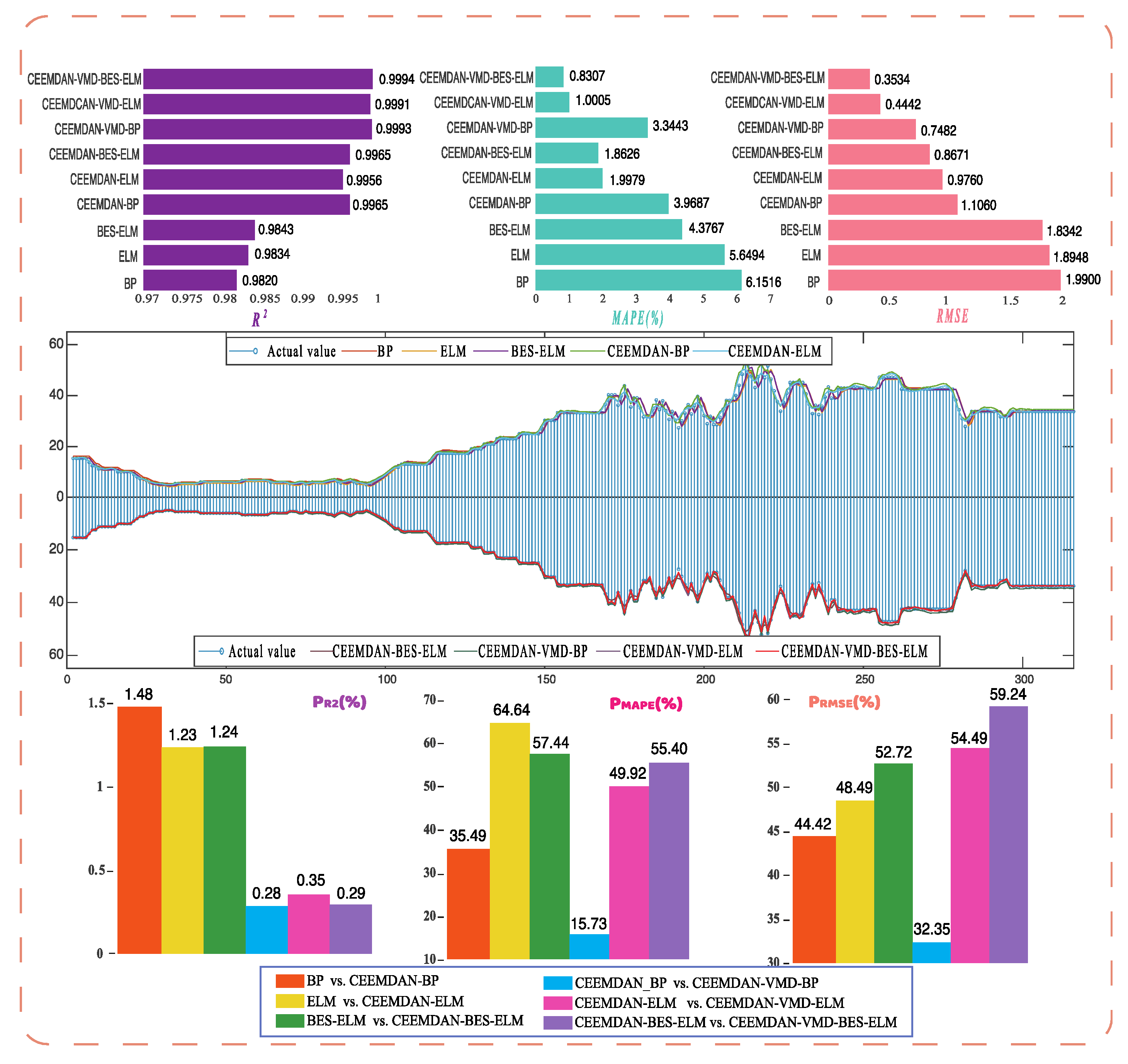
Comparing all evaluation indicators, CEEMDAN-VMD-BES-ELM has excellent predictive performance. The proposed model has the highest $R^2$value, the lowest $MAPE$ and $RMSE$ values, which are 0.9938, 0.3987, and 0.1667 respectively.

(B)

When the individual models are combined with CEEMDAN, the prediction accuracy of the former has been greatly improved. For example, for the BP model, the $R^2$, $MAPE$, and $RMSE$ are 0.8925, 1.5164, and 0.7075, respectively. However, the three indicators of CEEMDAN-BP are 0.9566, 1.1724, and 0.4564, and the corresponding improvement percentage indicators are 7.19%, 22.69%, and 35.50% respectively. Comparing ELM and CEEMDAN-ELM, $P_{R^2}$, $P_{MAPE}$, and $P_{RMSE}$ are 7.57%, 32.25%, and 41.08%, respectively. For BES-ELM and CEEMDAN-BES-ELM, the former’s $R^2$ increased by 8.09%, $MAPE$ decreased by 36.74%, and $RMSE$ decreased by 45.55%.

(C)

Comparing the model combined CEEMDAN-EMD with the model combined CEEMDAN, the former has better prediction performance. For CEEMDAN-ELM, the $R^2$, $MAPE$, and $RMSE$ are 0.9619, 0.9799, and 0.4146, respectively. However, the three values to CEEMDAN-VMD-ELM are 0.9919, 0.4373, and 0.1914 respectively. The corresponding three improvement percentage index values are 3.12%, 55.37%, and 53.84%.

(D)

Comparing the BES-ELM model with the ELM model, the former has a stronger ability to capture sequence features. For ELM, $R^2$, $MAPE$, and $RMSE$, the values are 0.8942, 1.4463, and 0.7038 respectively. However, the three values of BES-ELM are 0.8968, 1.4190, and 0.6835 respectively. Similarly, comparing CEEMDAN-ELM with CEEMDAN-BES-ELM, CEEMDAN-VMD-ELM, and CEEMDAN-VMD-BES-ELM, the model fused with ELM optimized by BES has better prediction accuracy.

4.2.2. Guangdong Carbon Market

Using the actual data collected from the Guangdong carbon market as an example to conduct an empirical analysis, the prediction results and the evaluation index values are displayed in Figure 7. Based on the figure, the same analyses as Hubei carbon market could be obtained.

4.2.3. Shenzhen Carbon Market

The actual data were collected from the Shenzhen carbon market as an example to conduct an empirical analysis. Among them, the prediction results and indicators of SZA-2015 are shown in Figure 8, and the results of SZA-2013 and SZA-2014 are shown in Figure A1 and Figure A2, respectively. Based on the figure, the same analyses as those of the Hubei carbon market could be obtained.

In summary, through empirical analysis of the five actual datasets in the above three carbon markets, the following conclusions could be drawn:

(A)

In the empirical analysis of all datasets, the CEEMDAN-VMD-BES-ELM constructed in this paper is the best in any evaluation indicators, which fully demonstrates that the proposed model proposed is robust and suitable for carbon price prediction.

(B)

When the single model is compared with the corresponding model combined with CEEMDAN, the latter is more competitive in prediction results and evaluation criteria. It may be because the inherent complexity of the carbon price time series has been weakened after being processed by CEEMDAN, reducing the difficulty of forecasting, which illustrates the suitability of the introduction of data preprocessing methods to process carbon price data.

(C)

After the introduction of the secondary decomposition algorithm, through the comparison of the prediction accuracy of the corresponding models, it is obvious that the model combined with CEEMAN-VMD has a more satisfactory forecasting accuracy than the model combined with CEEMDAN. It demonstrates that the reprocessing of IMF1 obtained by decomposing CEEMDAN could break through the limitation of accuracy and predict the carbon price more effectively.

(D)

It is necessary to optimize ELM output weights and hidden layer thresholds through BES. According to the experimental results, whether it is ELM, CEEMDAN-ELM, or CEEMDAN-VMD-ELM, the models optimized by BES predict superior performance, that is, BES-ELM is better than ELM, CEEMDAN-BES-ELM is better than CEEMDAN-ELM, and CEEMDAN-VMD-BES-ELM is better than CEEMDAN-VMD-ELM. Hence, BES could improve the stability of ELM and better capture the non-linear characteristics of the carbon price.

5. Conclusions and Discussion

Accurate and reliable carbon price forecasting is of great significance to ensure the smooth operation of the carbon market. This paper presents a novel carbon price prediction model of CEEMDAN-VMD-BES-ELM. To cope with the complexity of the carbon price time series, a two-stage decomposition algorithm combining CEEMDAN and VMD is applied to process the data. At the same time, considering that the random setting of ELM weights and thresholds will affect the stability of the model, the meta-heuristic search algorithm BES is utilized to optimize the parameters. The prediction performance of the proposed model will be compared with the comparison model, including BP, ELM, BES-ELM, CEEMDAN-BP, CEEMDAN-ELM, CEEMDAN-BES-ELM, CEEMDAN-VMD-BP, and CEEMDAN-VMD-ELM, in the empirical analysis of five actual datasets. The results show the following:

(1)

The prediction accuracy of CEEMDAN-VMD-BES-ELM in the empirical analysis is the most prominent of all models, which fully reflects the excellent robustness and prediction performance of the proposed model, which is suitable for carbon price forecasting.

(2)

The experimental results show that CEEMDAN could effectively decompose the carbon price and improve the prediction accuracy of the model. Taking the Hubei carbon market as an example, after combining with CEEMDAN, the $R^2$ of BES-ELM increased by 8.09%, the $MAPE$ decreased by 36.74%, and the $RMSE$ decreased by 45.55%. Obviously, CEEMDAN decomposes the original carbon price into more stable subsequences, making the prediction more accurate. This conclusion is also confirmed by Lu et al. [38].

(3)

The novel secondary decomposition algorithm CEEMDAN-VMD is introduced into the field of carbon price prediction, which significantly improves the forecasting performance of the model. The highly volatile IMF1 was decomposed by VMD into more regular component sequences, which reduces the difficulty of prediction and improves the prediction accuracy [27,39]. The experimental results prove that CEEMDAN-VMD could effectively extract the complex characteristics of carbon price and further break through the limitation of accuracy.

(4)

Faced with the instability caused by the randomness of output weights and hidden layer thresholds to ELM, it is necessary to apply optimization algorithms to determine the best values of its parameters [40,41]. Therefore, in this paper, the BES algorithm is applied to select the optimal combination of ELM parameters. The experimental results indicate that the model combined with BES-ELM could better capture the volatility of the carbon price and has better forecasting performance.

Although the proposed model in this paper has excellent prediction performance, there is still room for improvement. Since the carbon price time series is chaotic, many factors affect its fluctuations, but the input variables of the model in this study are only historical data. Future work will explore the impact of some factors such as policy measures, climate environment, and related energy prices on the results of carbon price predictions. In addition, the model has high prediction accuracy and robustness, and it can further explore its applications in other fields.

References

1. Hashim, H.; Ramlan, M.R.; Shiun, L.J.; Siong, H.C.; Kamyab, H.; Majid, M.Z.A.; Lee, C.T. An Integrated Carbon Accounting and Mitigation Framework for Greening the Industry. Energy Procedia 2015, 75, 2993–2998. [Google Scholar] [CrossRef] [Green Version]
2. Huang, Y.; He, Z. Carbon price forecasting with optimization prediction method based on unstructured combination. Sci. Total Environ. 2020, 725, 138350. [Google Scholar] [CrossRef]
3. Lotze, H.K.; Tittensor, D.P.; Bryndum-Buchholz, A.; Eddy, T.D.; Cheung, W.W.L.; Galbraith, E.D.; Barange, M.; Barrier, N.; Bianchi, D.; Blanchard, J.; et al. Global ensemble projections reveal trophic amplification of ocean biomass declines with climate change. Proc. Natl. Acad. Sci. USA 2019, 116, 12907–12912. [Google Scholar] [CrossRef] [Green Version]
4. Zhao, C.; Liu, B.; Piao, S.; Wang, X.; Lobell, D.B.; Huang, Y.; Huang, M.; Yao, Y.; Bassu, S.; Ciais, P.; et al. Temperature increase reduces global yields of major crops in four independent estimates. Proc. Natl. Acad. Sci. USA 2017, 114, 9326–9331. [Google Scholar] [CrossRef] [Green Version]
5. Carrão, H.; Naumann, G.; Barbosa, P. Global projections of drought hazard in a warming climate: A prime for disaster risk management. Clim. Dyn. 2018, 50, 2137–2155. [Google Scholar] [CrossRef] [Green Version]
6. Park, S.-Y.; Sur, C.; Lee, J.-H.; Kim, J.-S. Ecological drought monitoring through fish habitat-based flow assessment in the Gam river basin of Korea. Ecol. Indic. 2020, 109, 105830. [Google Scholar] [CrossRef]
7. Sun, W.; Wang, Y. Factor analysis and carbon price prediction based on empirical mode decomposition and least squares support vector machine optimized by improved particle swarm optimization. Carbon Manag. 2020, 11, 315–329. [Google Scholar] [CrossRef]
8. Song, Y.; Liu, T.; Liang, D.; Li, Y.; Song, X. A Fuzzy Stochastic Model for Carbon Price Prediction Under the Effect of Demand-related Policy in China’s Carbon Market. Ecol. Econ. 2019, 157, 253–265. [Google Scholar] [CrossRef]
9. Zhang, Y.; Zhang, J. Estimating the impacts of emissions trading scheme on low-carbon development. J. Clean. Prod. 2019, 238, 117913. [Google Scholar] [CrossRef]
10. Sun, W.; Zhang, C. Analysis and forecasting of the carbon price using multi—Resolution singular value decomposition and extreme learning machine optimized by adaptive whale optimization algorithm. Appl. Energy 2018, 231, 1354–1371. [Google Scholar] [CrossRef]
11. Tian, C.; Hao, Y. Point and interval forecasting for carbon price based on an improved analysis-forecast system. Appl. Math. Model. 2020, 79, 126–144. [Google Scholar] [CrossRef]
12. Hao, Y.; Tian, C.; Wu, C. Modelling of carbon price in two real carbon trading markets. J. Clean. Prod. 2020, 244, 118556. [Google Scholar] [CrossRef]
13. Wang, J.; Sun, X.; Cheng, Q.; Cui, Q. An innovative random forest-based nonlinear ensemble paradigm of improved feature extraction and deep learning for carbon price forecasting. Sci. Total Environ. 2021, 762, 143099. [Google Scholar] [CrossRef]
14. Benz, E.; Trück, S. Modeling the price dynamics of CO2 emission allowances. Energy Econ. 2009, 31, 4–15. [Google Scholar] [CrossRef]
15. Koop, G.; Tole, L. Forecasting the European carbon market. J. R. Stat. Soc. Ser. A 2013, 176, 723–741. [Google Scholar] [CrossRef] [Green Version]
16. Fan, X.; Li, S.; Tian, L. Chaotic characteristic identification for carbon price and an multi-layer perceptron network prediction model. Expert Syst. Appl. 2015, 42, 3945–3952. [Google Scholar] [CrossRef]
17. Zhu, B.; Han, D.; Wang, P.; Wu, Z.; Zhang, T.; Wei, Y.-M. Forecasting carbon price using empirical mode decomposition and evolutionary least squares support vector regression. Appl. Energy 2017, 191, 521–530. [Google Scholar] [CrossRef] [Green Version]
18. Han, M.; Ding, L.; Zhao, X.; Kang, W. Forecasting carbon prices in the Shenzhen market, China: The role of mixed-frequency factors. Energy 2019, 171, 69–76. [Google Scholar] [CrossRef]
19. Zhu, B.; Wei, Y. Carbon price forecasting with a novel hybrid ARIMA and least squares support vector machines methodology. Omega 2013, 41, 517–524. [Google Scholar] [CrossRef]
20. Sun, G.; Chen, T.; Wei, Z.; Sun, Y.; Zang, H.; Chen, S. A Carbon Price Forecasting Model Based on Variational Mode Decomposition and Spiking Neural Networks. Energies 2016, 9, 54. [Google Scholar] [CrossRef] [Green Version]
21. Chevallier, J. Wavelet packet transforms analysis applied to carbon prices. Econ. Bull. 2011, 31, 1731–1747. [Google Scholar]
22. Zhu, B. A Novel Multiscale Ensemble Carbon Price Prediction Model Integrating Empirical Mode Decomposition, Genetic Algorithm and Artificial Neural Network. Energies 2012, 5, 355–370. [Google Scholar] [CrossRef]
23. Zhou, J.; Yu, X.; Yuan, X. Predicting the Carbon Price Sequence in the Shenzhen Emissions Exchange Using a Multiscale Ensemble Forecasting Model Based on Ensemble Empirical Mode Decomposition. Energies 2018, 11, 1907. [Google Scholar] [CrossRef] [Green Version]
24. Zhu, J.; Wu, P.; Chen, H.; Liu, J.; Zhou, L. Carbon price forecasting with variational mode decomposition and optimal combined model. Phys. A Stat. Mech. Appl. 2019, 519, 140–158. [Google Scholar] [CrossRef]
25. Sun, W.; Huang, C. A carbon price prediction model based on secondary decomposition algorithm and optimized back propagation neural network. J. Clean. Prod. 2020, 243, 118671. [Google Scholar] [CrossRef]
26. Sun, S.; Wei, L.; Xu, J.; Jin, Z. A New Wind Speed Forecasting Modeling Strategy Using Two-Stage Decomposition, Feature Selection and DAWNN. Energies 2019, 12, 334. [Google Scholar] [CrossRef]
27. Peng, T.; Zhou, J.; Zhang, C.; Zheng, Y. Multi-step ahead wind speed forecasting using a hybrid model based on two-stage decomposition technique and AdaBoost-extreme learning machine. Energy Convers. Manag. 2017, 153, 589–602. [Google Scholar] [CrossRef]
28. Sun, W.; Huang, C. A novel carbon price prediction model combines the secondary decomposition algorithm and the long short-term memory network. Energy 2020, 207, 118294. [Google Scholar] [CrossRef]
29. Huang, N.E. The empirical mode decomposition and the hilbert spectrum for nonlinear and non-stationary time series analysis. Proc. R. Soc. Lond. 1998, 454, 903–995. [Google Scholar] [CrossRef]
30. Wu, Z.H.; Huang, N.E. Ensemble empirical mode decomposition: A noise-assistant data analysis method. Adv. Adapt. Data Anal. 2009, 1, 1–41. [Google Scholar] [CrossRef]
31. Torres, M.E.; Colominas, M.A.; Schlotthauer, G.; Flandrin, P. A complete ensemble empirical mode decomposition with adaptive noise. In Proceedings of the 2011 IEEE International Conference on Acoustics, Speech and Signal Processing (ICASSP), Prague, Czech Republic, 22–27 May 2011; pp. 4144–4147. [Google Scholar] [CrossRef]
32. Dragomiretskiy, K.; Zosso, D. Variational Mode Decomposition. IEEE Trans. Signal Process. 2014, 62, 531–544. [Google Scholar] [CrossRef]
33. Alsattar, H.A.; Zaidan, A.A.; Zaidan, B.B. Novel meta-heuristic bald eagle search optimisation algorithm. Artif. Intell. Rev. 2019, 53, 2237–2264. [Google Scholar] [CrossRef]
34. Zhou, J.; Huo, X.; Xu, X.; Li, Y. Forecasting the Carbon Price Using Extreme-Point Symmetric Mode Decomposition and Extreme Learning Machine Optimized by the Grey Wolf Optimizer Algorithm. Energies 2019, 12, 950. [Google Scholar] [CrossRef] [Green Version]
35. Dégerine, S.; Lambert-Lacroix, S. Characterization of the partial autocorrelation function of nonstationary time series. J. Multivar. Anal. 2003, 87, 46–59. [Google Scholar] [CrossRef] [Green Version]
36. Liu, X.; Zhou, X.; Zhu, B.; He, K.; Wang, P. Measuring the maturity of carbon market in China: An entropy-based TOPSIS approach. J. Clean. Prod. 2019, 229, 94–103. [Google Scholar] [CrossRef]
37. Qi, S.; Wang, B.; Zhang, J. Policy design of the Hubei ETS pilot in China. Energy Policy 2014, 75, 31–38. [Google Scholar] [CrossRef]
38. Lu, H.; Ma, X.; Huang, K.; Azimi, M. Carbon trading volume and price forecasting in China using multiple machine learning models. J. Clean. Prod. 2020, 249, 119386. [Google Scholar] [CrossRef]
39. Rahimpour, A.; Amanollahi, J.; Tzanis, C.G. Air quality data series estimation based on machine learning approaches for urban environments. Air Qual. Atmos. Health 2021, 14, 191–201. [Google Scholar] [CrossRef]
40. Ding, J.; Chen, G.; Yuan, K. Short-Term Wind Power Prediction Based on Improved Grey Wolf Optimization Algorithm for Extreme Learning Machine. Processes 2020, 8, 109. [Google Scholar] [CrossRef] [Green Version]
41. Liu, Z.-F.; Li, L.-L.; Tseng, M.-L.; Lim, M.K. Prediction short-term photovoltaic power using improved chicken swarm optimizer-Extreme learning machine model. J. Clean. Prod. 2020, 248, 119272. [Google Scholar] [CrossRef]
Figure 1. The flowchart of the proposed model.
Sustainability 13 08413 g001
Figure 2. Proportion of carbon pilot trading volume.
Sustainability 13 08413 g002
Figure 3. (a) Original carbon price; (b) PACF results of the corresponding carbon market.
Sustainability 13 08413 g003
Figure 4. (a) Decomposition results of CEEMDAN in Hubei market; (b) PACF results of subsequences.
Sustainability 13 08413 g004
Figure 5. (a) VMD results of the IMF1; (b) PACF results of the corresponding sequence.
Sustainability 13 08413 g005
Figure 6. Prediction results of different models in the Hubei market.
Sustainability 13 08413 g006
Figure 7. Prediction results and evaluation index values in the Guangdong market.
Sustainability 13 08413 g007
Figure 8. Prediction results and evaluation index values in SZA-2015.
Sustainability 13 08413 g008