Article

Spatial Heterogeneity of Factors Influencing CO2 Emissions in China’s High-Energy-Intensive Industries

1
School of Environment Science and Spatial Informatics, Chinese University of Mining and Technology, Xuzhou 221116, China
2
School of Geography and Environment, Shandong Normal University, Jinan 250358, China
*
Authors to whom correspondence should be addressed.
Sustainability 2021, 13(15), 8304; https://doi.org/10.3390/su13158304
Submission received: 23 June 2021 / Revised: 18 July 2021 / Accepted: 20 July 2021 / Published: 25 July 2021

Abstract

:
In recent years, China has overtaken the United States as the world’s largest carbon dioxide (CO2) emitter. CO2 emissions from high-energy-intensive industries account for more than three-quarters of the total industrial carbon dioxide emissions. Therefore, it is important to enhance our understanding of the main factors affecting carbon dioxide emissions in high-energy-intensive industries. In this paper, we firstly explore the main factors affecting CO2 emissions in high-energy-intensive industries, including industrial structure, per capita gross domestic product (GDP), population, technological progress and foreign direct investment. To achieve this, we rely on exploratory regression combined with the threshold criteria. Secondly, a geographically weighted regression model is employed to explore local-spatial heterogeneity, capturing the spatial variations of the regression parameters across the Chinese provinces. The results show that the growth of per capita GDP and population increases CO2 emissions; by contrast, the growth of the services sector’s share in China’s gross domestic product could cause a decrease in CO2 emissions. Effects of technological progress on CO2 emissions in high-energy-intensive industries are negative in 2007 and 2013, whereas the coefficient is positive in 2018. Throughout the study period, regression coefficients of foreign direct investment are positive. This paper provides valuable insights into the relationship between driving factors and CO2 emissions, and also gives provides empirical support for local governments to mitigate CO2 emissions.

1. Introduction

Over the past 20 years, global warming has become a serious issue, attracting increasing attention from the international community. Relative to pre-industrial levels, the impacts of global warming increases the temperature by 1.3 °C [1]. As a result, accompanied with an increase in temperature, glacier melting has caused sea levels to rise, and extreme weather events occur more frequently. Furthermore, it is widely accepted that increasing amounts of carbon dioxide (CO2) emissions significantly contribute to global warming. Since the period of reform and opening-up in 1978, China’s economy has grown at an average annual rate of 7 percent. Since 2008, China has overtaken the United States as the world’s largest CO2 emitter, and accounted for 23% of global CO2 emissions (CEs). As the largest developing country in the world, China has made a commitment that CEs will peak in 2030, and then CEs per unit of GDP will fall by between 60% and 65% compared with 2005 level. Why does China produce so many CEs? Largely due to the fact that high-energy-intensive (HEI) industries still account for a large proportion of the economy [2,3]. A previous study shows CEs from HEI industries account for 80% of total industrial CEs [4].
In China, HEI industries include petroleum refining and coking, mining industries, chemical production and processing, non-metallic mineral products, ferrous metals production, non-ferrous metal manufacturing, power generation and heating. China’s extraordinary economic development, since 1978, has occurred as a result of urbanization. By late 2017, about 60% of the total population lived in China’s urban areas; improving the living standards of the people, urbanization still continues to occur at a high rate [5,6,7]. However, in turn, it also increases the demands for more energy, building materials, and chemical products. Meanwhile, China is the world’s most important manufacturer and supplier of industrial products and living goods. In general, this requires more HEI industries, and inevitably contributes to more carbon dioxide emissions. The Chinese government has formulated the 13th Five-Year Plan to ensure the completion of the low-carbon development tasks and to achieve China’s carbon emission peak by 2030. Undoubtedly, as the main pillar industries of China’s national economy, HEI industries must improve their energy efficiency and, in turn, reduce CEs. Therefore, understanding the key driving factors of CEs will contribute to developing energy-saving plans and CEs reduction policies. In addition, China is a vast country, and its various regions have obvious differences with regard to natural resources, production conditions and technical levels. Thus, when this paper investigates the factors that influence factors of carbon emissions, the spatial heterogeneity of China’s regions is taken into consideration. Additionally, long-term and short-term spatial effects are also important to explore in considering the relationships between the influencing factors and CEs.
To explore the pathway of CEs reduction in HEI industries, many scholars have carried out research on the driving factors of CEs and measures to reduce CEs in different regions or industries [8,9,10,11]. In power-generation and heating industries, some previous studies have indicated a percentage increase in non-fossil fuel energy leads to a certain percentage decrease in CEs from the electricity-generation sector among different countries or regions [9,12]. Lin and Tan [13] found that the average rates from CEs growth in China’s energy-intensive industries were roughly 7.20% between 1985 and 2014, and identified that industrial-scale and labor productivity were the main driving factors in increasing CEs, while energy intensity had a negative effect on CEs. Lin and Wang [14] explored the CEs and mitigation potential from iron and steel industries among different provinces in China during 2000–2011, and suggested that technical innovation and low-carbon investment should play an important role in mitigating CEs. Wu, et al. [15] identified the reasons for recent no-growth in CEs, and deduced that China’s CEs in most of HEI industries have peaked or approached the peak in recent years. Griffin, et al. [16] explored some of the opportunities and challenges in reducing CEs in the chemical sector in the United Kingdom; the results showed that technological innovation was needed to meet the short-term and long-term goals for general emission reduction.
As mentioned previously, most of the CEs in China come directly from industrial production, especially energy-intensive industries [13]. Therefore, it is important to identify which factors affect CEs in HEI industries. Many scholars have examined the main factors affecting CEs [11,17,18,19,20]. These factors include the level of economic development, energy intensity, industrial structure, urbanization level, energy mix, population, technological progress, foreign trade, foreign direct investment, energy sector investment, and so on [10,11,17,18,19,21]. Which of these are the main factors affecting carbon emissions in energy-hungry industries?
Additionally, the research approaches are also key to evaluate the effects of driving factors on CEs. A number of scholars developed a mathematical model between CEs and the driving factors to help local governments to formulate a reasonable CEs reduction policy. Since 1971,Ehrlich and Holdren have developed the IPAT model which suggests environment impact (I) is a function of population (P), affluence (A) and technology (T) [22,23]; in turn, many studies have since employed the extended STIRPAT model, based on the classical IPAT, to evaluate the main driving factors for CEs [8,24,25]. Additionally, the LMDI (Logarithmic Mean Divisia Index) model is also a popular method applied to investigate the main influencing factors of CEs. Ren, et al. [26] employed the LMDI method to explore the impacts of the main driving factors on CEs and found that an increase in economic output contributed to an increase in CEs in China’s manufacturing industries. Similarly, Xu, et al. [27] used the LMDI model to investigate the factors of CEs, and contended that economic output was the most important driver of CEs.
In addition, a number of previous studies use spatial-econometric analysis to explore the effects of driving factors on CEs. For example, Yang, Zhou, Poon and He [22] employed three spatial-autoregressive models including the spatial-lag model (SLM), the spatial-error model (SEM) and the spatial Durbin model (SDM), to reveal the relative significance of drivers on the intensity of CEs in eight regions. The spatial-dependence effects are considered in the three models above, which can indicate both positive and negative spatial fill-over effects on different regions. Wang and Li [12] used the SDM model to estimate the direct and indirect spatial effects of non-fossil fuel power generation on CEs, and the result of the spatial panel analysis showed that a higher share of non-fossil fuel power generation contributed to reducing CEs both in terms of direct and indirect spatial effects. However, these models, which belong to the global regression model, are only able to evaluate global parameters for a regression model. In recent years, the geographically weighted regression (GWR) method has been employed to explore local-spatial heterogeneity and capture the spatial variations of the regression parameters across different regions [19,28,29,30,31].
In this study, and to the best of our knowledge, the GWR method is employed to analyze the relationships between CEs in HEI industries and its driving factors, and to explore the spatial heterogeneity of these factors. At the same time, this study also helps to understand the role the driving factors play in influencing CEs in HEI industries. In this paper, firstly, spatial autocorrelation is used to analyze the spatial characteristics of CEs in HEI industries between Chinese provinces. Then, we employ exploratory regression to determine the major driving factors of CEs in HEI industries. Furthermore, the GWR model is used to explore the driving factors of province-level CEs by providing different parameter sets across neighboring provinces. Finally, we compare the different impacts of every driving variable on CEs in different provinces.

2. Data Sources and Methods

2.1. Data Sources and Description

Based on data availability, we selected 30 provinces in China as our study areas. Four provincial districts including Tibet, Hong Kong, Macau, and Taiwan, are excluded due to the lack of complete data. The study period covers the years from 2007 to 2018. The energy consumption data are obtained from China Energy Statistical Yearbook (2008–2019), and the datasets of the driving factors are available at the provincial level from China Statistical Yearbook (2008–2019). The gross industrial output value of HEI industries is acquired from the China Industrial Economic Statistical Yearbook (2008–2019). CEs are measured based on the formula of CEs in the Intergovernmental Panel on Climate Change (IPCC) [32]. Whether practical or theoretical perspectives, determining which variables in a model are its most important predictors is critical [33]. Based on the previous literature, ten potential driving factors of CEs in HEI industries are selected, these factors include population (POP), per capita gross domestic product (PGDP), urban level (UL), industrial structure (IS), technological progress (TP), foreign trade (FT), foreign direct investment (FDI), energy sectors investment (ESI), energy mix (EM), and energy intensity (EI).
In order to reduce the effects of inflation during the entire study period, gross domestic product (GDP) is converted into constant prices based on the Chinese 2000 price level. Energy intensity (EI) is a leading indicator of economic data which is measured by the quantity of energy required per unit of GDP, urbanization level (UL) is calculated as urban population divided by the total population, energy mix (EM) is calculated as coal use divided by total energy use, the energy sectors investment (ESI) refers to investment amounts in energy sectors at the provinces level, which is acquired from China Energy Statistical Yearbook, and we employ Solow Growth Model to calculate the value of technological progress (TP). In addition, industrial structure (IS) refers to the services sector’s share in China’s gross domestic product.

2.2. Study Methods

Spatial-autocorrelation method is widely used to evaluate the spatial dependency and heterogeneity among different objects, and the most popular test of spatial autocorrelation is the global Moran’s index test. The formula of Moran’s Index is expressed as follows:
M o r a n s   I = n i = 1 n j = 1 n w i j ( x i x ¯ ) ( x j x ¯ ) i = 1 n ( x i x ¯ ) 2 i = 1 n j = 1 n w i j
where x i represents the observation in the i-th location, x j represents the observation in the j-th location, x ¯ is the average of all observations for every attribute feature, x i , in n locations. w i j is an element of the spatial weights matrix, w, used to reflect the neighboring relationship among different regions at n positions [19].
Local-spatial autocorrelation analysis could mainly explore the distribution pattern of individual unit attribute values in a heterogeneous space, and this analysis could measure the degree of local-spatial correlation between each unit and its surrounding units [34]. The formula of the local-spatial autocorrelation Index is expressed as follows:
I = n ( x i x ¯ ) j = 1 n w i j ( x j x ¯ ) i = 1 n ( x i x ¯ )
where I represent the spatial autocorrelation Index, x i and x j represent the observation in the i-th location and the j-th location respectively, and w i j is an element of the spatial weights matrix. A positive I means that a high value’s neighbors have high values, or a low value’s neighbors have low values. A negative I implies that a low value’s neighbors are more likely to have high values, or vice versa [35].
When there are many potential explanatory variables that might be important contributing factors to the response variable, finding the relative importance of predictor variables is important for building regression models. The exploratory regression is similar to the stepwise regression, evaluating all possible combinations of the input candidate explanatory variables along with threshold criteria, these criteria include adjusted R2, coefficient p-values, Variance Inflation Factor (VIF) values, Jarque-Bera p-values.
The geographically weighted regression (GWR) model could be widely used to explore the spatial variation of regression parameters. Compared with the general linear models, the GWR model is a local form of the generalized linear regression, which could construct separate linear regressions for every geographical unit. In general, the GWR method extends OLS linear regression models by accounting for the spatial autocorrelation of variables and estimating a separate model and local parameter for each geographic location in the dataset, based on a local sub-dataset which uses a differential spatial weight matrix [36]. The GWR model can be represented as:
y i = β 0 ( u i , v i ) + j = 1 k β j ( u i , v i ) x i j + ε i
where y i represents CEs in HEI industries at i-th location of provincial unit(LPU) k is the number of independent variables, x i j represents the j-th independent variable at the i-th LPU, ( u i , v i ) is the geographical coordinate of the i-th LPU, β j ( u i , v i ) represents the locally estimated coefficient of the j-th independent variable at the i-th LPU, which is a function of geographical location. β 0 ( u i , v i ) is the intercept at the i-th LPU, ε i is the error term. Based on the distance-weighted least square regression method, the coefficient of the GWR model at each site are estimated by
β ^ ( u i , v i ) = ( X T W ( u i , v i ) X ) 1 X T W ( u i , v i ) Y
where β ^ ( u i , v i ) is the vector of estimated coefficients at the i-th LPU, X is the matrix of independent variables, Y is the n×1 vector of the dependent variable, and W ( u i , v i ) is n × n spatial weight matrix:
w ( u i , v i ) = [ w i 1           0                         0   0             w i 2                     0                                             0             0               0             0             w i n ]
Due to different distances between the provinces, the key of the GWR model is to calculate the bandwidth or the number of neighbors used in every location. To obtain the optimal number of neighboring provinces selected, the Akaike Information Criterion (AIC) was chose. The bi-square weighting function was used to calculate the weight between the provinces, and it can be expressed as follows:
W i j = { [ 1 ( d i j d max ) 2 ] 2                   f o r       d i j < d max             0                                                   o t h e r w i s e
where d max denotes the max distance from the n-th farthest provinces to the regression province.

3. Results

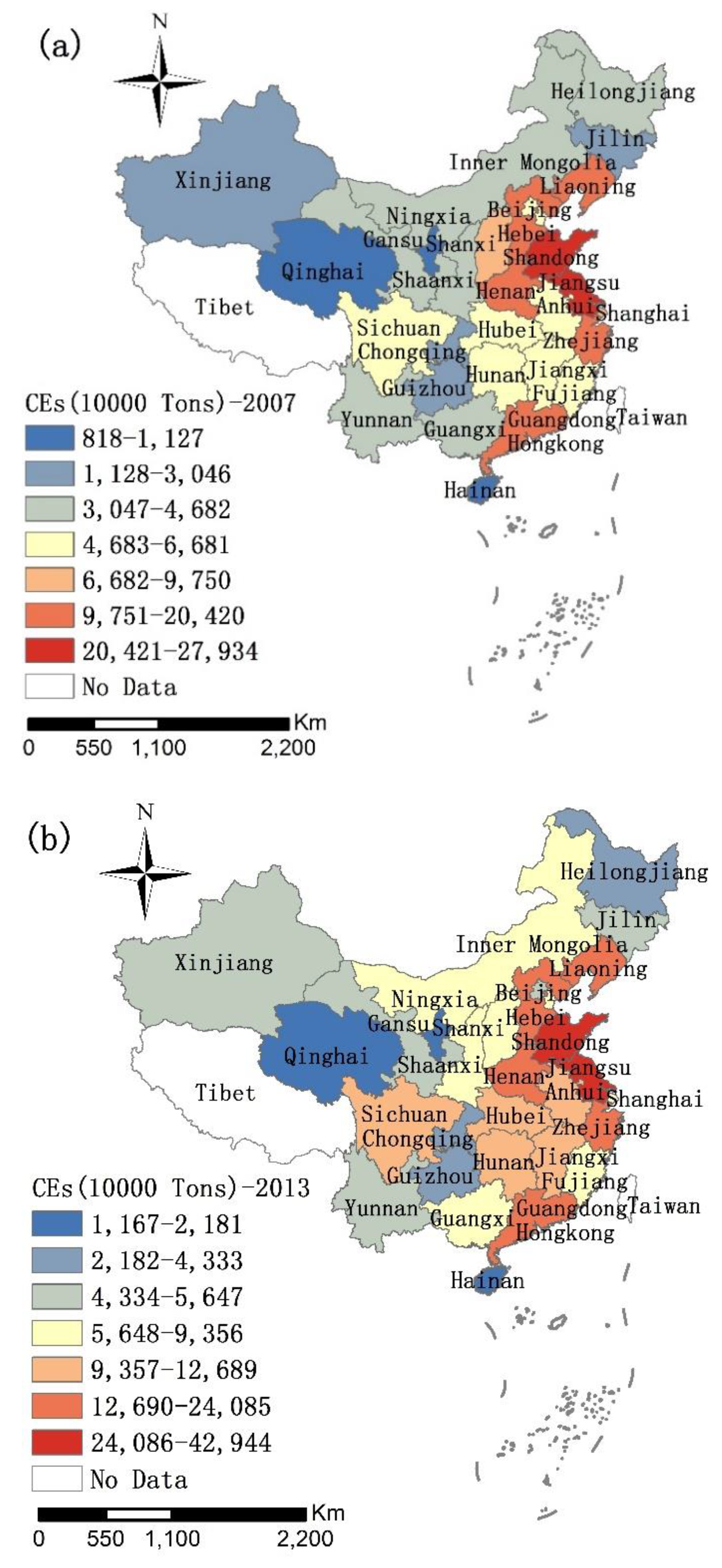
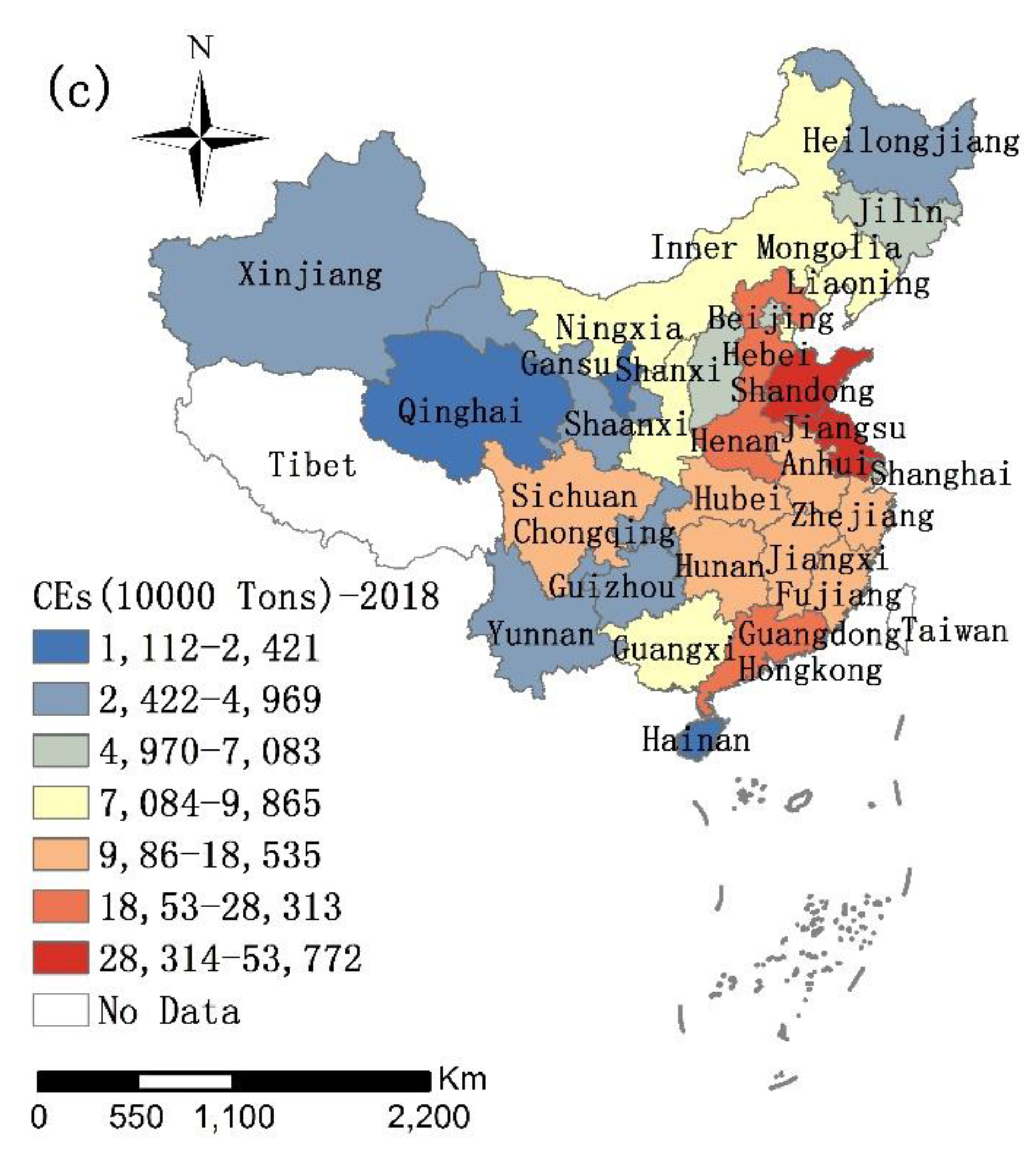
3.1. Temporal and Spatial Heterogeneity of CEs

In this study, we investigate the spatial heterogeneity of CEs in HEI industries in 2007, 2013 and 2018. Figure 1 shows the temporal and spatial distributions of CEs across the entirety of China. From the perspective of space, the distribution difference in CEs is very clear. The top two carbon dioxide emitters are Shandong and Jiangsu, and the three smallest emitters are located in northwestern and southern regions, mainly including Hainan, Qinghai and Ningxia. Shandong remains China’s largest emitter of carbon dioxide, contributing 12.0%, 12.3% and 14.4% of total national emissions in the three different years, respectively, while Hainan is always China’s smallest emitter of carbon dioxide, occupying 2.9%, 0.3% and 0.3%. From a temporal perspective, CEs are about 2334 Mton in 2007, while they rise 59.6%, to 3,725 Mton, in 2018. As the top two carbon dioxide emitters, Shandong and Jiangsu are responsible for 23.9% of the national CEs in 2007, unexpectedly accounting for more than 26.6% in 2018. In contrast, the three smallest emitters only occupy 1.2% and 1.5% in 2007 and 2018, respectively.
On the whole, the provinces with enormous carbon emissions are mainly distributed throughout China’s eastern coastal regions. In recent years, the CEs of central provinces have also been increasing. The main reason for this is that China’s extensive development model of high consumption and high pollution has not been fundamentally changed. Although the export-oriented development model has made tremendous contributions to China’s rapid economic development, it has shown little regard for the environment and, in turn, lead to over-exploitation of resources and CEs. The Chinese government should establish the “rules of the game”, including property rights, patent protections, and incentives to invest in technological innovation. These rules contribute to low economic growth, which would therefore encourage the institution of a sustainable economic development model.

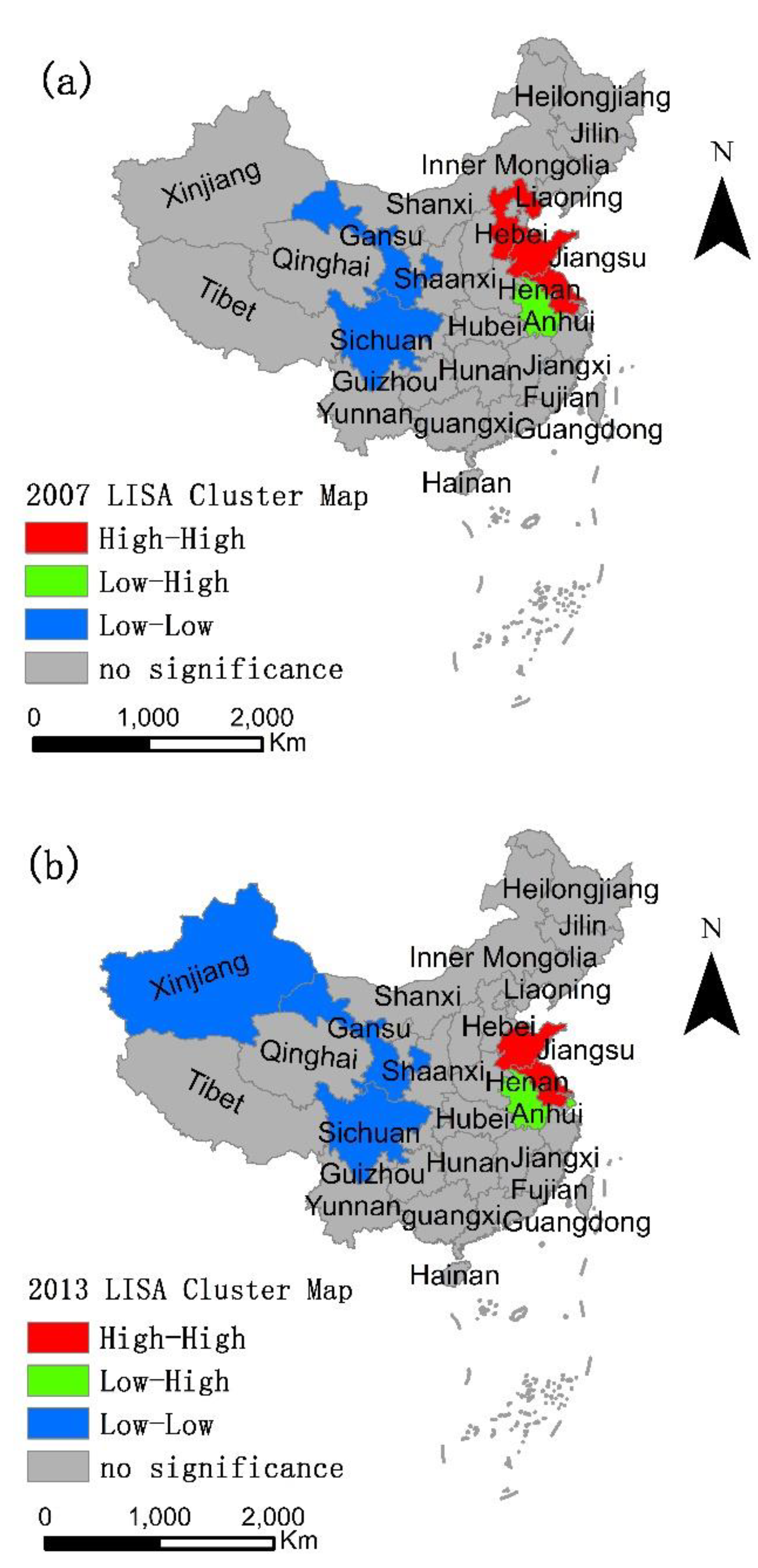
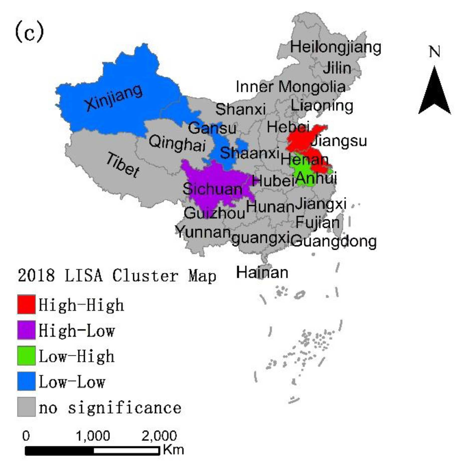
3.2. Spatial Autocorrelation Analysis of CEs in HEI Industries

Before performing the GWR model, we use Moran’s I to examine whether there is a spatial autocorrelation between the CEs in HEI industries. The Moran’s Index in 2007, 2013, and 2018 are given in Table 1. The results show that global Moran’s Index are greater than 0.3 over the whole time period, suggesting that there is significantly positive spatial autocorrelation in the CEs between provinces in HEI industries.
Local indicators of spatial association (LISA) indicate the high-high and low-low locations (positive local-spatial autocorrelation) are typically spatial clusters. High-High locations are usually called hot spots (locations where high-attribute values are surrounded by high-attribute values: High-High); Low-Low locations are cold spots (locations where low-attribute values are surrounded by low-attribute values: Low-Low). The High-Low and Low-High locations (negative local-spatial autocorrelation) are considered as spatial outliers. As is shown in Figure 2, High-High, Low-Low, High-Low and Low-High regions are found at the 5% level of significance. During the whole period, four or five provinces fall into High-High and Low-Low spatial clusters. Meanwhile, a few provinces fall in Low-High and High-Low areas, which reflects the existence of positive spatial autocorrelation. Shandong and Jiangsu provinces are always in High-High zones, while Gansu province is in Low-Low zones over the whole period. This reveals that Shandong and Jiangsu provinces, and their neighboring provinces, emit more carbon dioxide in HEI sectors. In contrast, Gansu and its neighboring provinces emit less CEs. Interestingly, High-High clusters do not include Guangdong province, which has the largest GDP among the 30 provinces in China; this suggests most of its neighboring provinces emit less carbon dioxide.

3.3. Evaluating All Possible Combinations of the Candidate Explanatory Variables

Exploratory regression is used to find major drivers of CEs in HEI industries. To eliminate the differences in numerical magnitude within the statistical data, we normalize all explanatory variables based on the average of these variables in 2007, 2013 and 2018, respectively. The following threshold criteria are set: acceptably adjusted R2 is more than 0.5, the p-value of Coefficient is less than 0.05, VIF value is less than 7.5, the p-value of Jarque-bera test is greater than 0.1.
Table 2 shows the results of exploratory regression, and lists seven models, with the highest adjusted R2 meeting all of the threshold criteria. These models are divided into four groups, by number of exploratory variables. The fourth group only contains one model which has five explanatory variables, and we note that the model has five variables that are statistically significant. Based on adjusted R2 and other threshold criteria, we decide to use IS, PGDP, TP, POP and FDI as explanatory variables, following the GWR model.

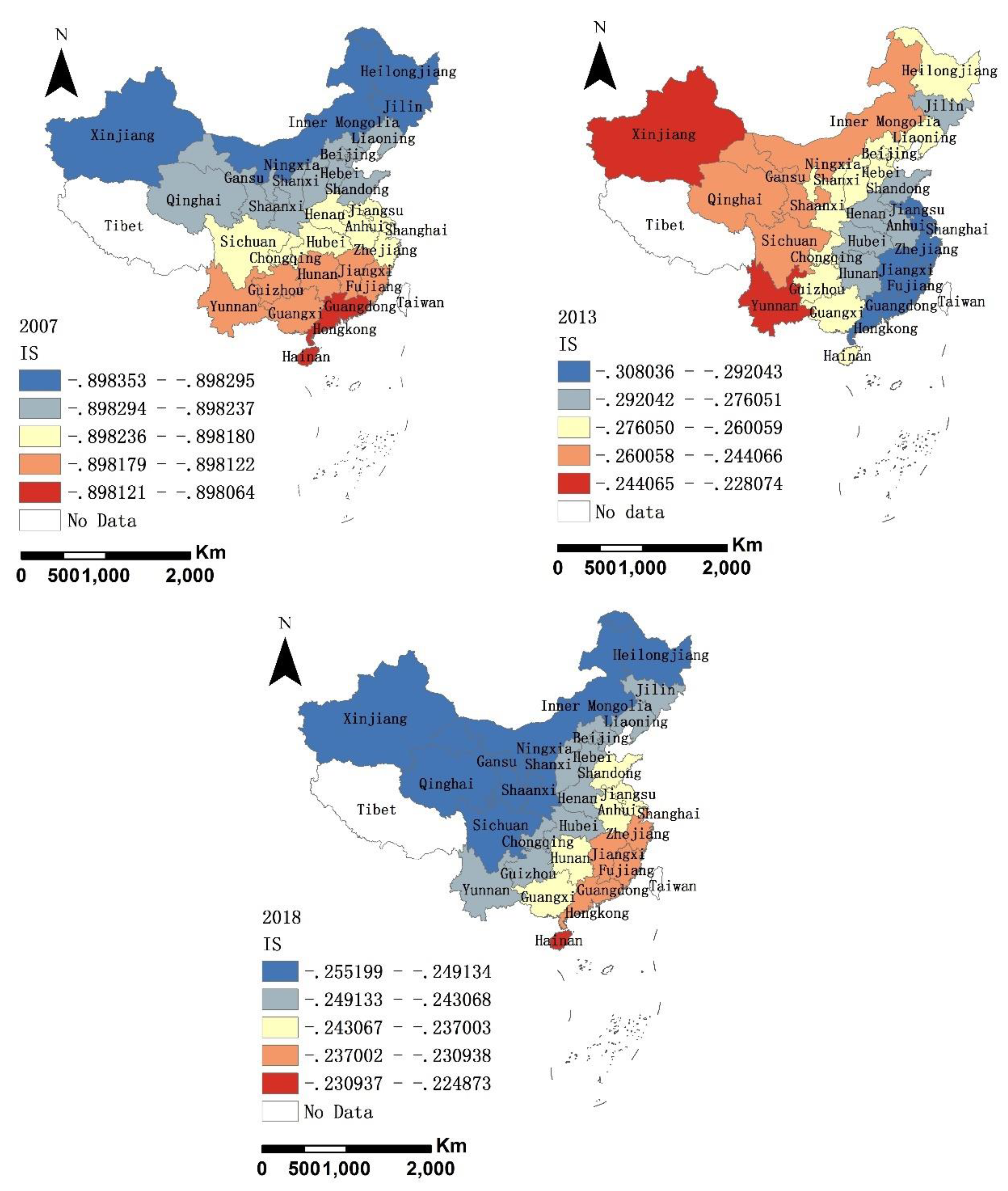
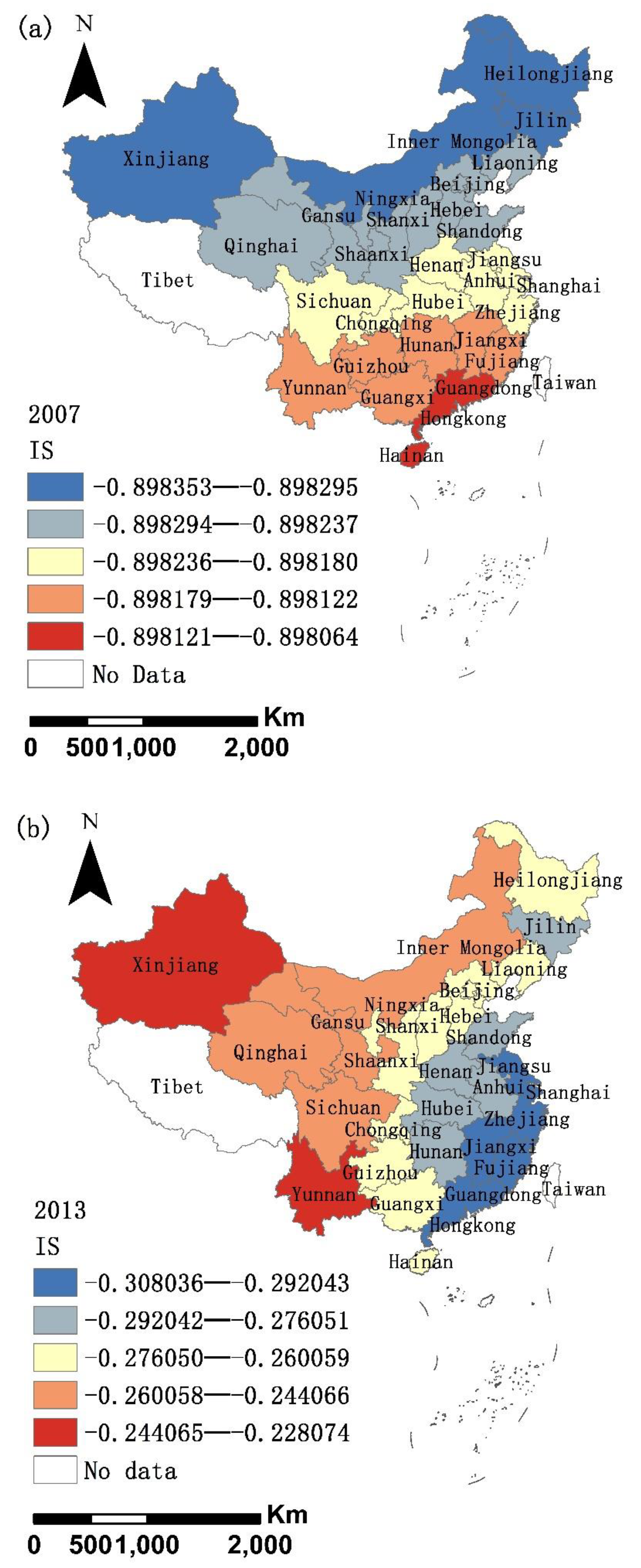
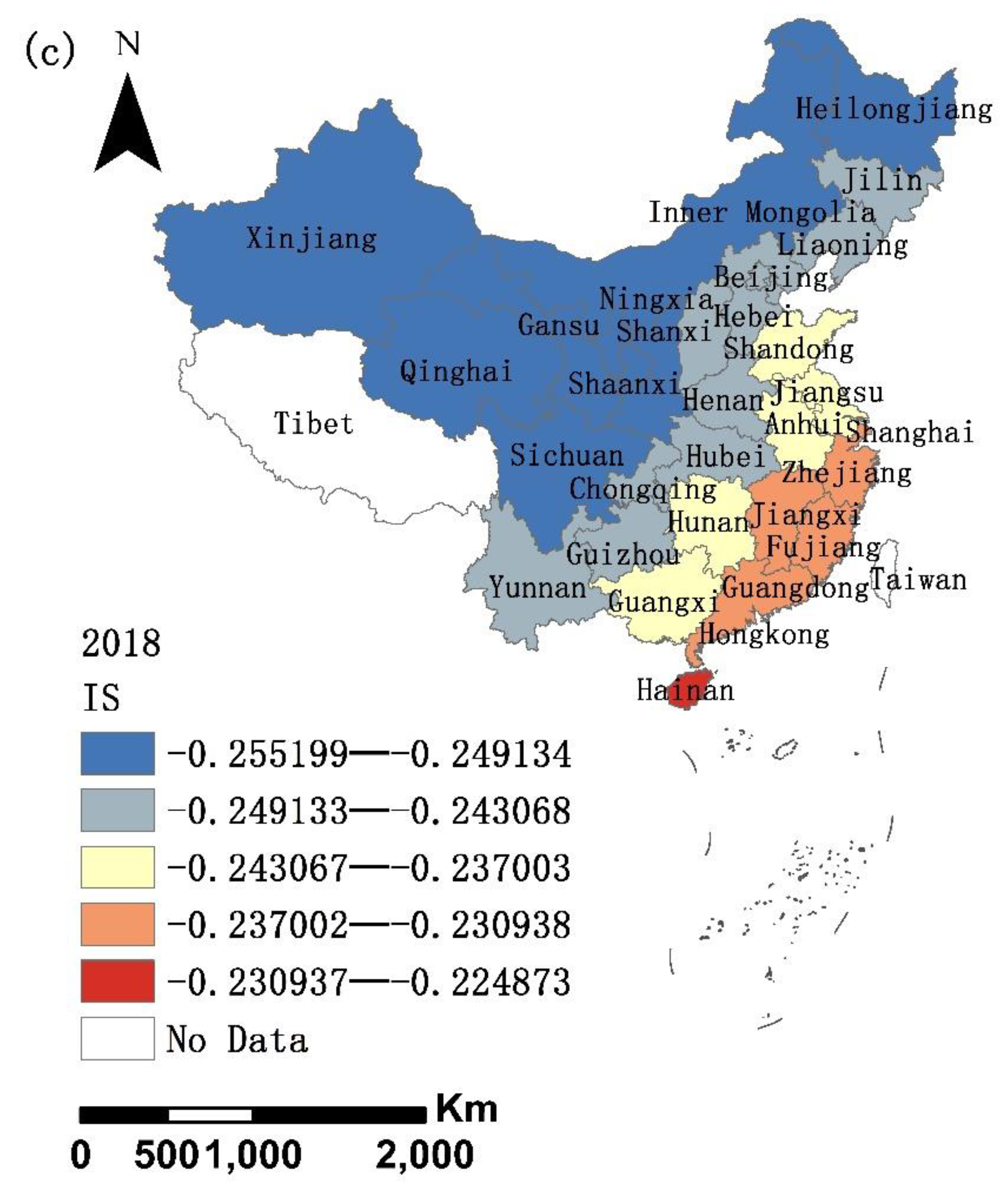
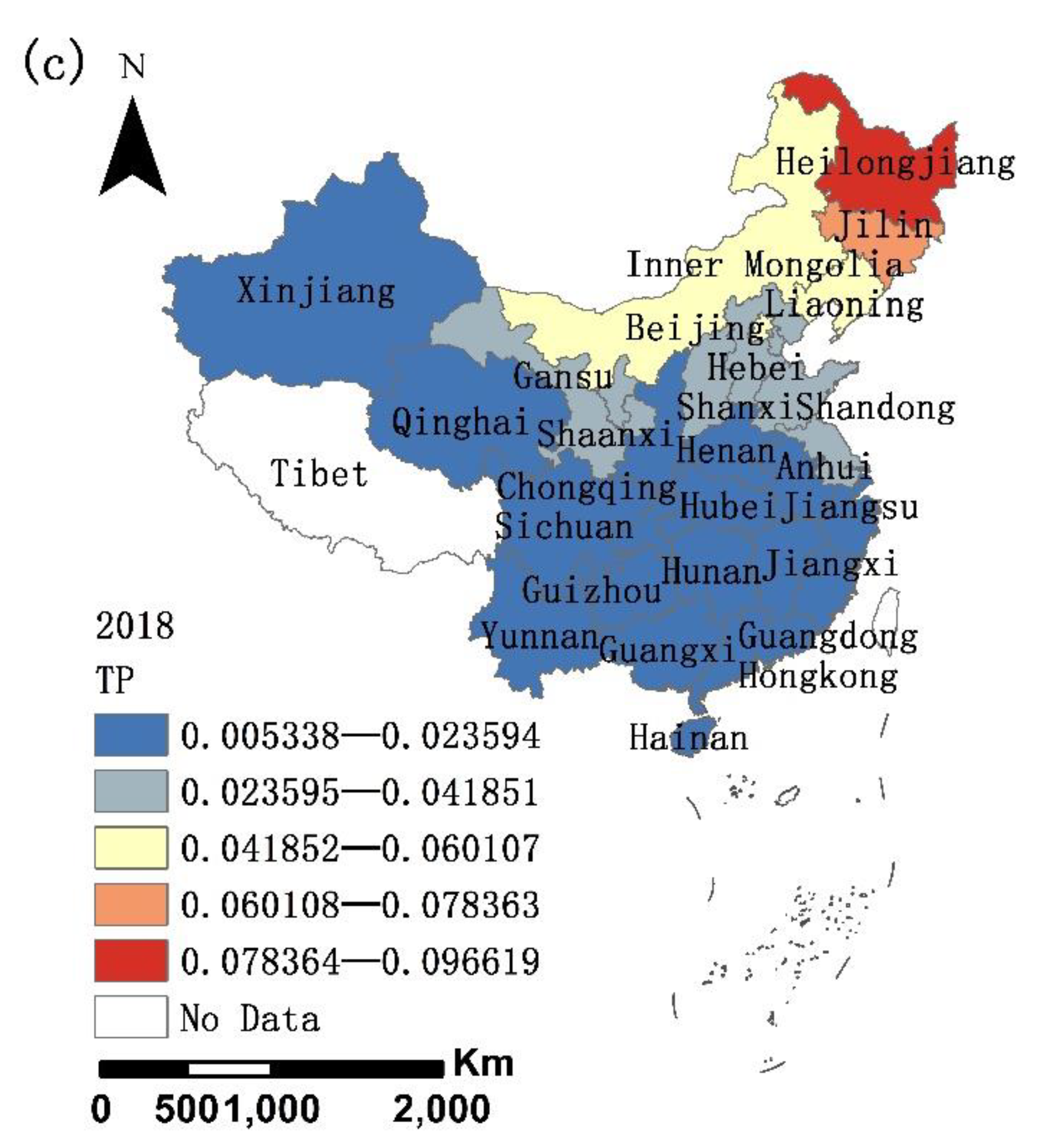
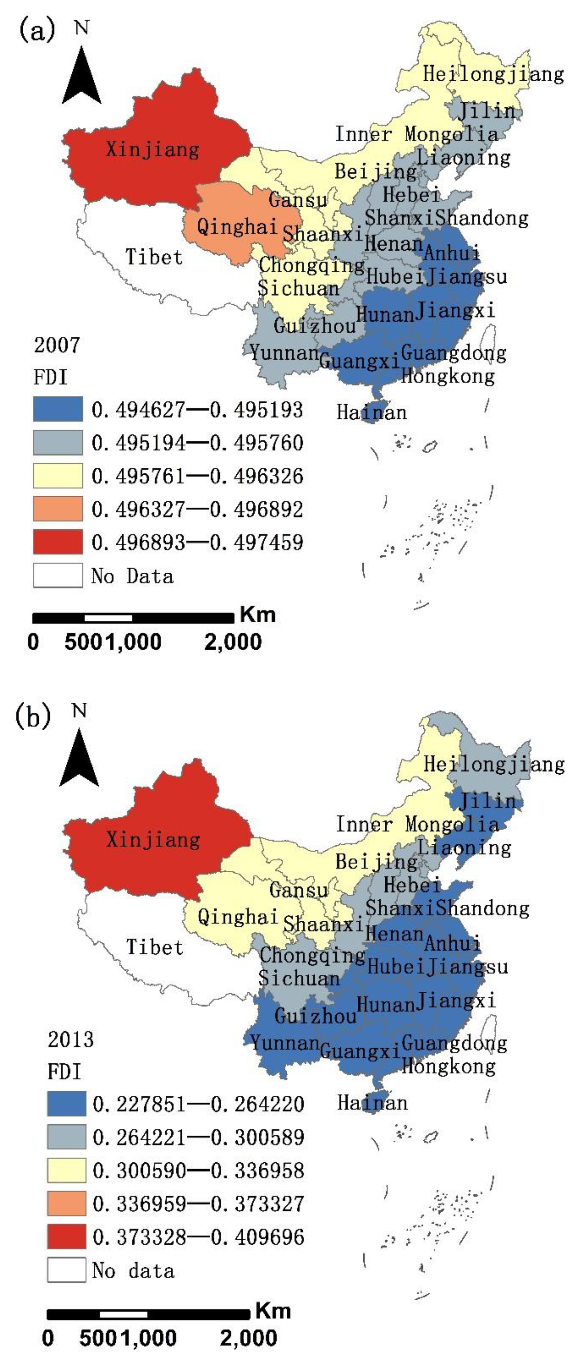
3.4. Estimation Results of the GWR Model

Table 3 shows the calculated results of the GWR models during three periods. The R square values identify spatial variation over the whole study area; those exceeding 0.8 indicate more than 80% of the variation and could be explained by IS, PGDP, TP, POP or FDI. As the GWR model constructs a separate linear regression for every province, regression coefficients could be separately calculated for each province. The regression coefficients of POP and PGDP are always positive, which indicates a positive relationship between the two driving factors and CEs in HEI industries, and also that POP and PGDP are the key factors which increase CEs. However, the regression coefficient of IS is negative, which shows a negative relationship between IS and CEs, and further that IS contributes to the decrease in CEs. In the two years of 2007 and 2013, regression coefficients of TP are also negative but, by contrast, the coefficients are positive in 2018. On the whole, regression coefficients of FDI are mostly positive, though there are a few negative coefficients in some provinces in 2018. Meanwhile, Table 3 shows the maximum and the minimum of regression coefficients from the GWR model, compared with the coefficients from Ordinary Least Squares (OLS) regression model during the three periods. Absolute values of the intercepts in all of models are very small, which vary between 0.0583 and 0.188. The differences of regression coefficients, based on the GWR model, are very obvious among the 30 provinces in 2013 and 2018, which indicates the spatial heterogeneity of relationships between driving factors and CEs in HEI industries. Similarly, this shows the GWR model might be more suitable than the OLS regression model in this study.
As shown in the Table 4 below, the Moran’s I of the residuals from the GWR are very small in 2007, 2013 and 2018. All of p–values are higher than 0.05 in the three years and are therefore not statistically significant. The z-tests indicate spatial distribution of residuals are the result of random spatial processes. Thus, it is reasonable that the above five variables are selected as explanatory variables in the GWR model.

4. Discussion

4.1. The Effect of the Industrial Structure on CO2 Emissions

It is evident from Figure 3 that IS has a strongly negative impact on CEs in HEI industries because many developed provinces have made great efforts to develop services and electronic-information industries, and also to limit HEI industries as much as possible in order to reduce CEs [37]. Compared with other independent variables, the effect of IS on CEs is relatively strong and gradually weakening. The averages of regression coefficients of IS in 2007, 2013 and 2018 are −0.8982, −0.2739 and −0.2437, respectively. In 2007, IS has great impact on CEs in the northern provinces, such as Inner Mongolia, Xinjiang. The reason for this is that the northern regions have a large number of HEI industries, the proportion of tertiary industries is small, thus resulting in more CEs. Compared with 2007, on the whole, regression coefficients of IS decline by 72.9 percent in 2018. Although China issued the 12th Five-Year Development Plan for Energy Saving and Environmental Protection Industry in 2012, and promoted the transformation of economic growth modes [38], the provinces of the western and northern China still develop HEI industries in order to best achieve their economic goals. Additionally, these provinces are mainly located in marginal areas, coupled with inconvenient transportation, which limits the development of service industries. Yet, eastern China experiences relatively low negative impacts of IS. These provinces, such as Guangdong, have a more developed industrial structure and thus avoid more CO2 emissions by importing high-energy-intensive products while exporting low-energy-intensive and higher-value-added products in the machinery, equipment and service sectors.
From 2007 to 2018, CEs in HEI industries have increased by about 59.6%, while the share of tertiary sectors in GDP rises slowly, climbing by 23.8%; this explains the phenomenon that the impact of IS on CEs in HEI industries is gradually weakening. However, a few results from previous studies are not consistent with the present study. For example, Liu et al. [39] found IS had positive effects on CEs in HEI industries, with coefficients of 0.179. Most previous studies identify that increasing the share of tertiary sectors in GDP contributes to reduction of CEs [37,40,41]. In the current and future period, the proportion of the third industry in the Chinese economy continues to rise. The provinces with high proportions of energy-intensive sectors should vigorously develop low-carbon industries and information industries to promote carbon emission reduction.

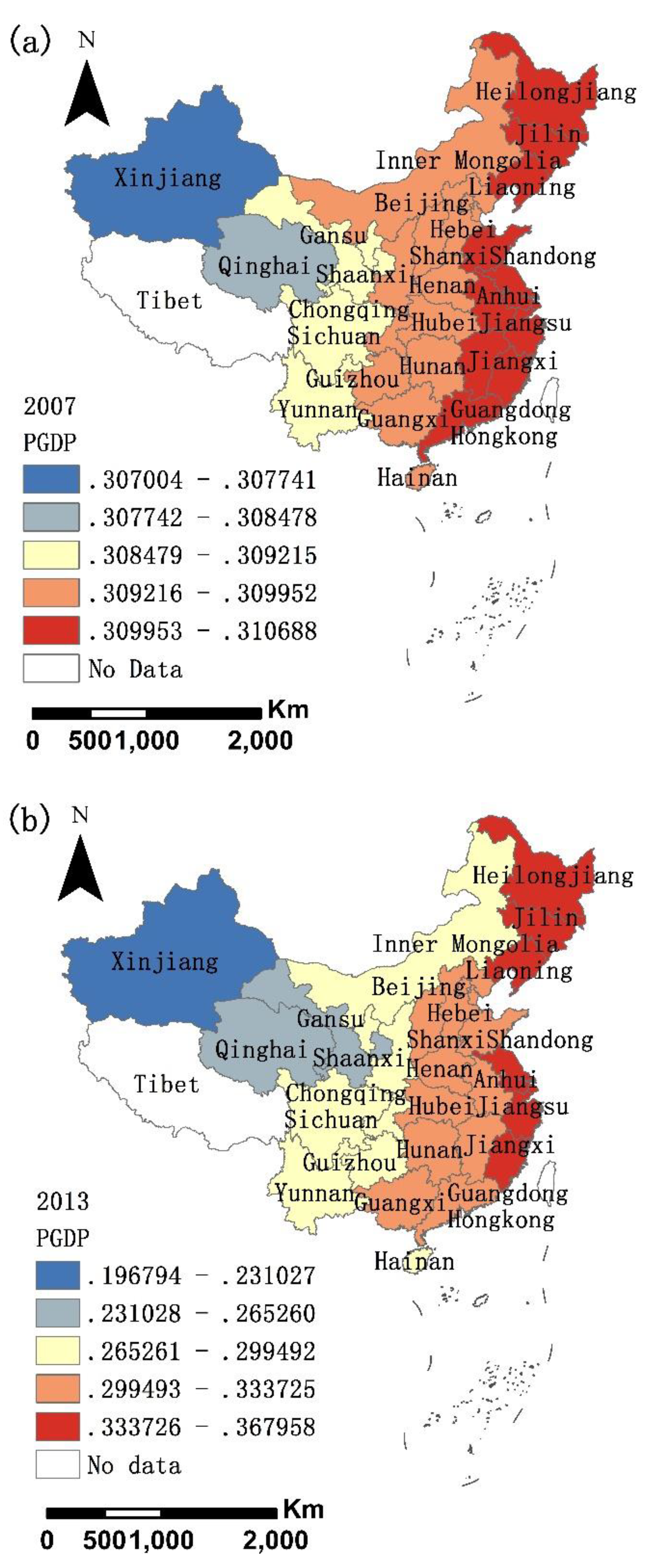
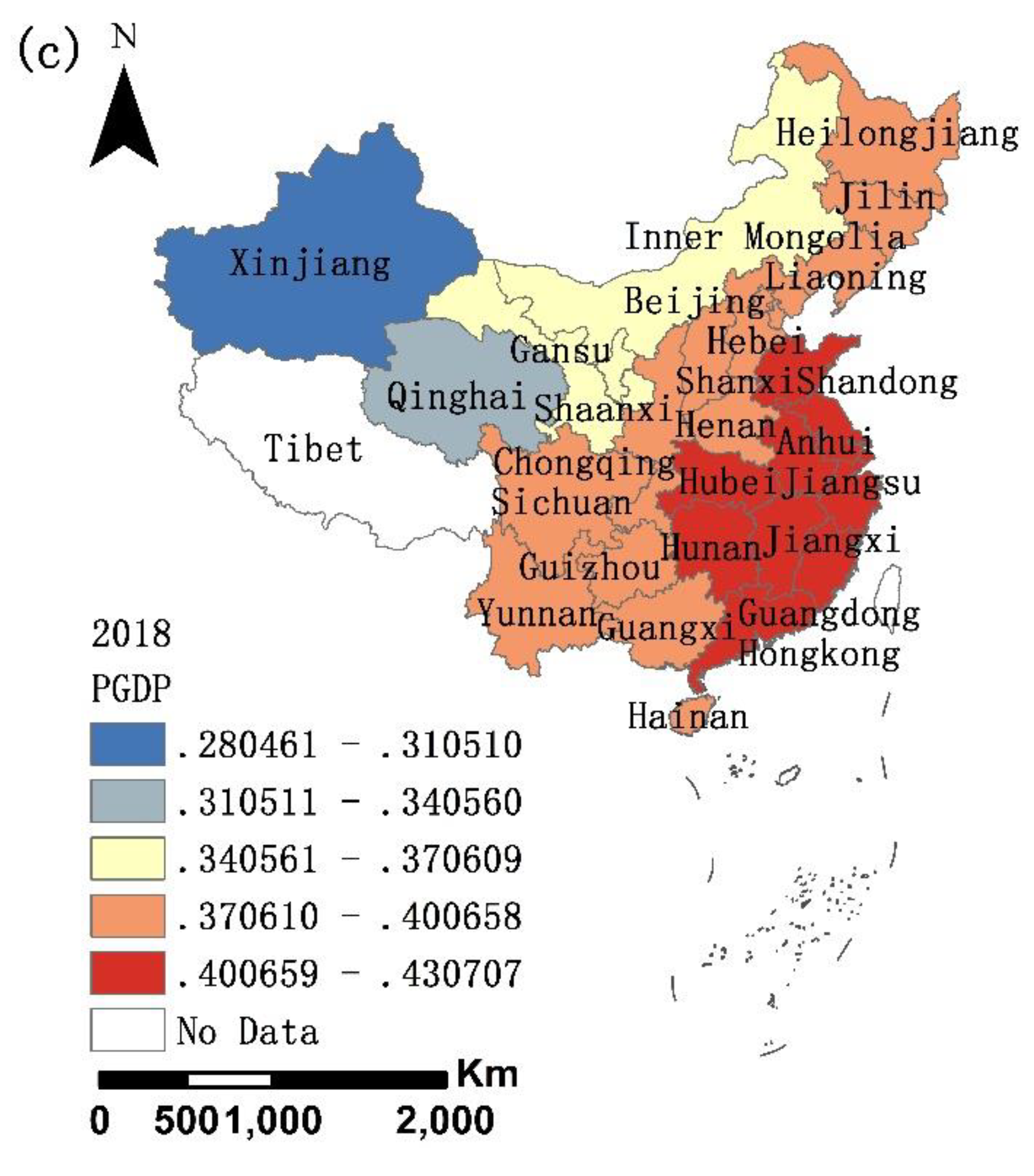
4.2. The Effect of the Per Capita GDP on CO2 Emissions

Figure 4 reflects the positive effects of per capita GDP on CEs in HEI industries in the different years. The regression coefficients range from 0.31 to 0.39 from 2007 to 2018. The groups of the regression coefficients of PGDP are similar across the different years. The regression coefficients are relatively low in western China but, by contrast, relatively high in eastern China. In 2007, the most influenced provinces are mainly distributed the in three northeastern provinces and the eastern coastal provinces. By the year 2018, its distribution area has extended to some central provinces. In the whole study period, the low-coefficient group has always been in the western provinces. Since the late 1970s, China has been one of the world’s fastest-growing economies and PGDP is also growing at faster rate. In the coverage of the 30 provinces, PGDP grows from 22,300 Yuan in 2007 to 59,100 Yuan in 2018. The growth of PGDP leads to the substantial increase of individual income, which in turn results in rising demand for energy products [19]. The results from the GWR model show that PGDP has the largest impact on the eastern coastal regions, because PGDP or individual income are higher in these regions than other regions. This suggests that these regions have greater potential to reduce CEs. In fact, economically developed provinces are characterized by higher than average CEs. Therefore, they have the responsibilities and obligations to reduce CEs.

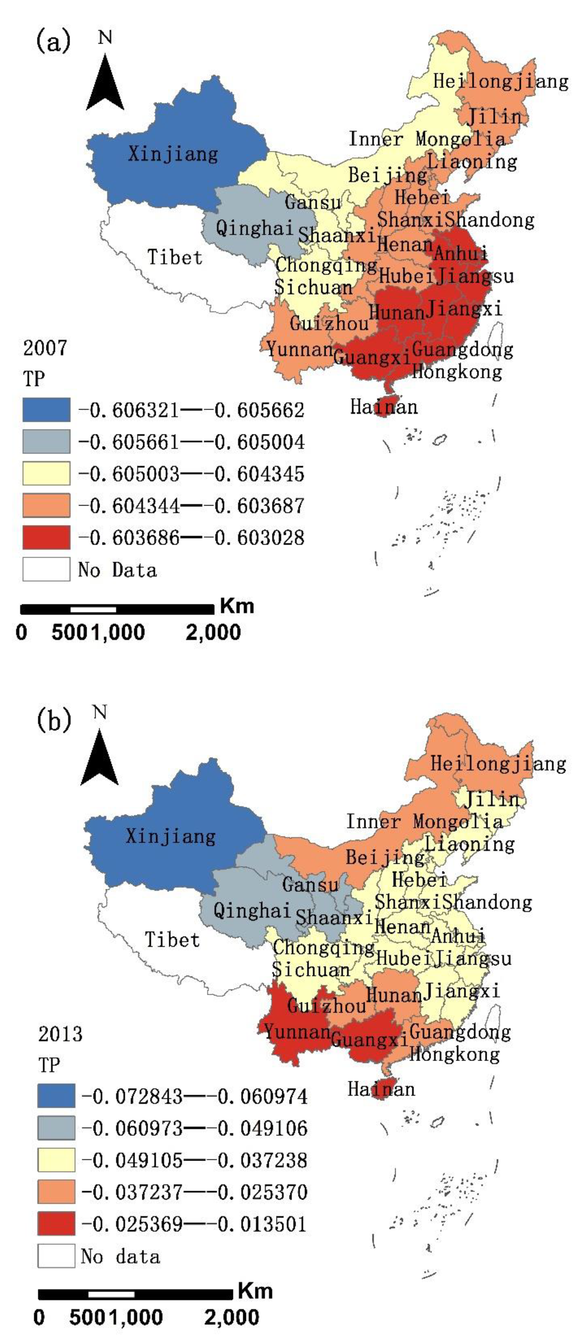
4.3. The Effect of the Technological Progress on CO2 Emissions

As is shown in Figure 5, technological progress has more significant impact on CEs in HEI industries in 2007 than in 2013 and 2018. Effects of TP on CEs in HEI industries are negative throughout the whole study period. From 2007 to 2018, the absolute average of regression coefficients on CEs declines from 0.60 to 0.03, and the result indicates the impact of TP on CEs is decreasing year by year. As a whole, the differences of regression coefficients between different provinces are small. This could mainly be attributed to TP increasing energy efficiency and reducing energy consumption [42]. While CEs will continue to steadily increase in the near future, TP will play a smaller role in reducing CEs, from the perspective of a purely mathematical model. Some previous studies have shown a negative relationship between TP and CEs. The finding in this study is somewhat consistent with the finding of Zhang et al. [43], who found that TP increased the efficiency of fossil fuel consumption and reduced CEs. However, a few researchers conclude that the relationship between TP and CEs is uncertain [42]. The main reasons for the inconsistent results may include differences in the calculation methods of technological progress, differences in estimating carbon emissions, and differences in mathematical model.

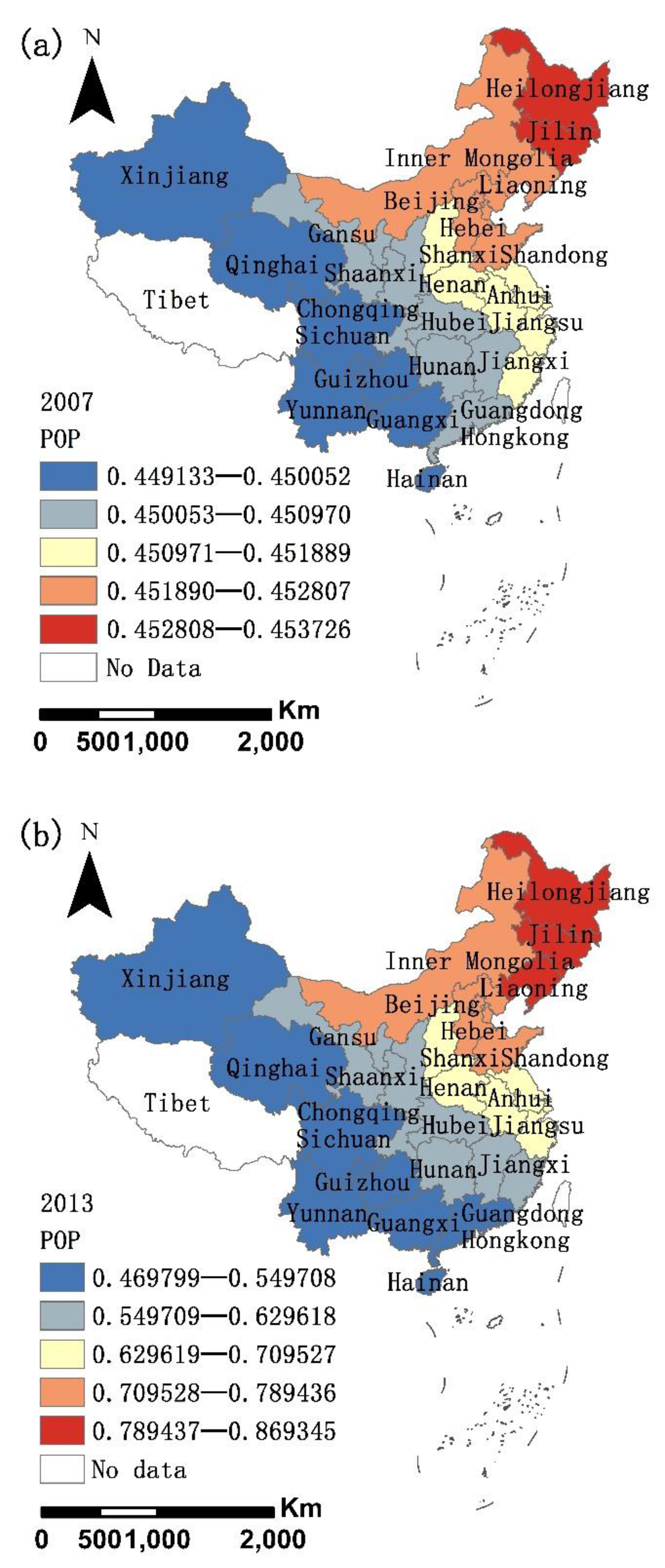
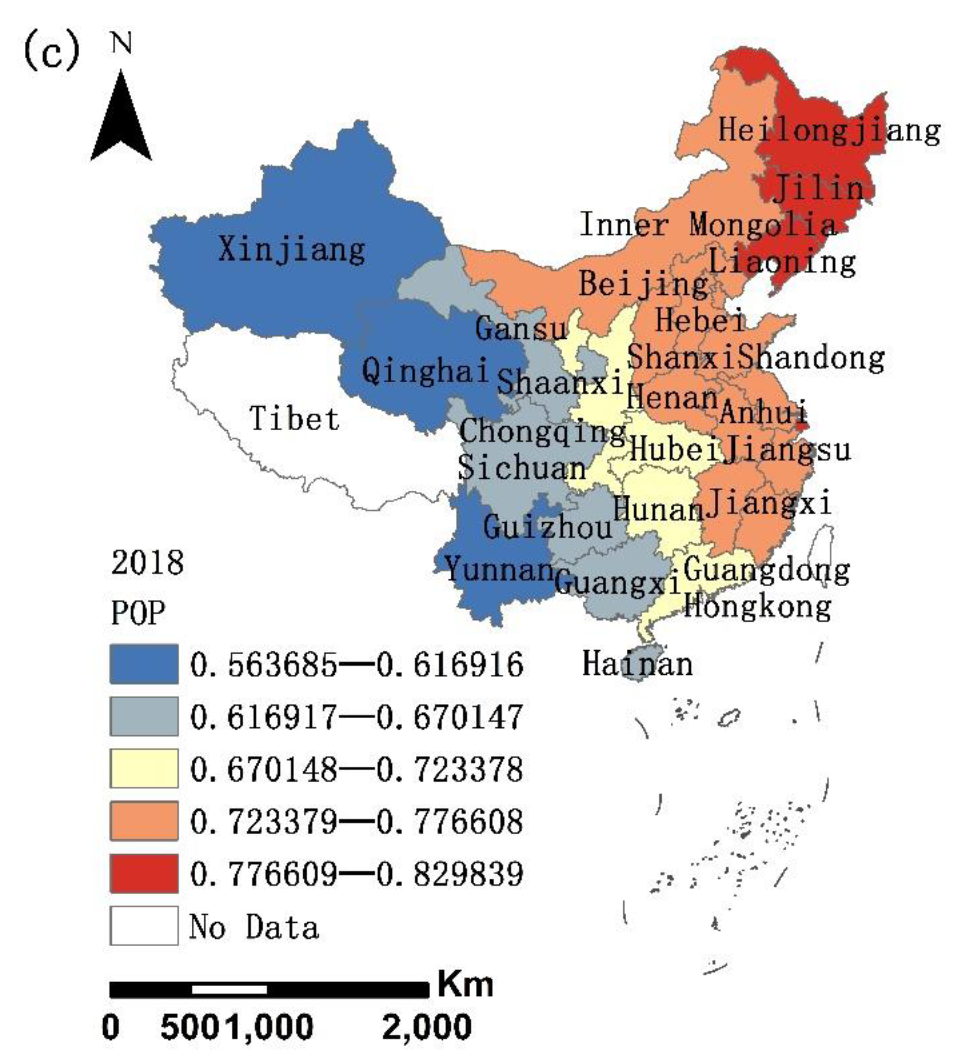
4.4. The Effect of the Population on CO2 Emissions

Figure 6 reveals that population is an important factor affecting CEs in HEI industries. The average regression coefficients of POP are 0.45, 0.64 and 0.71 in the three different years, respectively, which identifies that the positive effect of the population on CEs has increasingly grown from 2007 to 2018. The most affected provinces lie in the northeastern provinces, its maximum coverage includes Heilongjiang, Jilin and Liaoning in 2013 and 2018, and minimum coverage consists of Heilongjiang and Jilin in 2007. Small values of regression coefficients mainly distribute in the northwestern and southwestern provinces. Additionally, the regression coefficients of POP violently vary between provinces compared to the other four driving factors.
Population aging, urbanization and household size have distinct effects on CEs [44]. The population growth in China is slow across the whole study period, while the statistical data shows that urbanization rises from 32.6% to 59.8%. Urbanization is an important driving factor increasing CEs in HEI industries, as a great deal of the rural population migrates to cities each year to promote the rapid growth in the real estate industry [45]. This dramatic growth in the urban population would inevitably increase the demand for urban transportation, urban infrastructure, which relies on steel, cement, chemicals and other products. All of these products are processed and completed in high-energy-intensive industries, which contributes to emitting more CO2. Moreover, the average size of households in China varies between 2.8 and 3.1, and shrinking households contribute to an increase in CEs [46]. However, numerous studies have found that population aging contributed to reducing CEs [46,47].

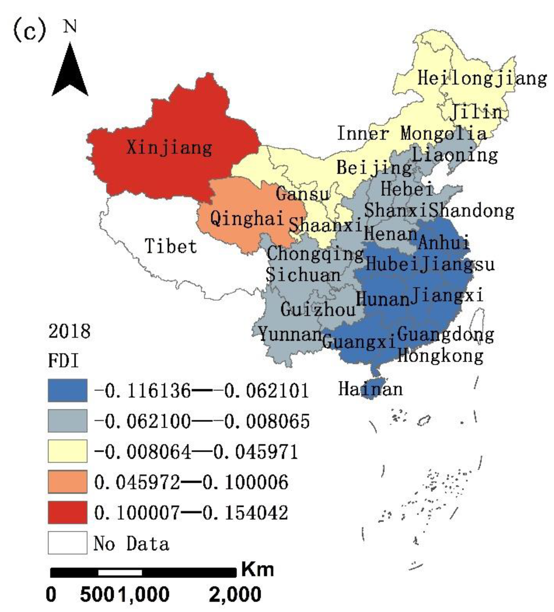
4.5. The Effect of the Foreign Direct Investment on CO2 Emissions

Figure 7 shows the effects of foreign direct investment on CEs falls gradually in 2007, 2013 and 2018. Although the boundaries between the groups are roughly northeast to southwest each year, the regression coefficients of FDI actually fluctuate very little among the provinces, especially in 2007. During three different years, the average regression coefficients of FDI are 0.50, 0.27 and −0.03, respectively, which indicates that the effect of FDI on CEs has gradually decreased. The most affected province is Xinjiang, located in northwestern part of China, and the least affected provinces mainly lie in the central and southeastern regions.
During the entire study period, China has remained the world’s second largest recipient of foreign direct investment. However, more than 20% of the total amount of FDI in the secondary industry flows into HEI industries between 2007 and 2018. There are several possible causes for this situation. Firstly, many local governments in China allow FDI in more HEI industries to increase taxes and promote the local economic growth. Secondly, the central and local government fails to amend its existing FDI industries guidance catalogue to encourage FDI to flow into low-carbon, high-tech sectors. Thirdly, the government has not formulated effective policies to guide foreign-funded enterprises to carry out technological innovation to reduce energy consumption per unit of GDP. The finding that FDI has positive impacts on CEs is consistent with previous research [48,49]. To date, the environmental problems caused by FDI has aroused great concern for the Chinese government.

5. Conclusions and Policy Implications

This study examines all possible combinations of the candidate influencing factors on CEs in HEI industries by employing the exploratory regression model. Based on adjusted R2 and other threshold criteria, IS, PGDP, TP, POP and FDI are selected as explanatory variables in the GWR model. The GWR model is then used to investigate the impact of the driving factors on CEs and their differences across the whole study area. The result reveals PGDP and POP are significantly positive driving factors on CEs. By contrast, IS has strongly negative impact on CEs. Meanwhile, effects of TP on CEs in HEI industries are negative in 2007 and 2013, while the coefficient is positive in 2018. On the whole, regression coefficients of FDI are positive, the coefficients are only negative in some provinces in 2018. The statistical data identifies the CEs are generally rising in HEI industries between 2007 and 2018. The differences of regression coefficients, based on the GWR model, are very obvious among the 30 provinces in 2013 and 2018, which indicates the spatial heterogeneity of relationships between driving factors and CEs in HEI industries.
Based on the empirical results of this work, the following corresponding policy implications are outlined below.
Firstly, optimizing and upgrading industrial structure is a powerful way to control CO2 emissions. The eastern provinces should further increase the proportion of the tertiary sector, optimize the energy-consumption structure and increase the use of renewable energy. Local governments should seek to develop high-tech service industries, such as computer, communications, semiconductor industries, and so on. The central and western provinces should vigorously develop characteristic agriculture, forestry, and tourism, in combination with their own resource advantages, and further promote the development of renewable energies such as wind power, hydropower and solar energy. In the meantime, these governments should make full use of financial support to further increase carbon sink through afforestation, desertification control to reduce CO2 emissions caused by industrial transfer.
Secondly, this study reveals that POP and PGDP are significantly positive driving factor on CEs. Wide disparities in population growth remain between different provinces in China. The more affluent coastal regions have had a large population inflow over the past 40 years; therefore, household registration policies need further improvement in order to control population sizes in the developed southeastern coastal regions. Meanwhile, the governments in the central and western regions should offer preferential taxation policies to create a better business climate and attract more enterprises to invest in the encouraged industries. In addition, various subsidies should be used to attract more talents for employment, and to induce labor transfers to the country’s west and northeast regions. The increase in PGDP is best way to measure economic growth, driving more consumption, including energy consumption. The local government should encourage people to adopt a low-carbon lifestyle. Taking daily life as an example, people can be encouraged to recycle all that they can, and also reduce food waste. The government sector should reward people who use public transit systems, especially bicycles.
Thirdly, our results indicate a positive relationship between FDI and CO2 emissions throughout most of the study period. This shows that Chinese government has excessively focused on economic development in the past 30 years. This policy stance is bound to cause great damage to the quality of the environment, and FDI is more concentrated in pollution-intensive and high-polluted industries. In recent years, the Chinese government has begun to encourage FDI in low-carbon industries, mainly focusing on the service sectors. In particular, the government should formulate and implement environmental regulations that force the firms receiving FDI to develop and use environmental protection technologies.
Fourthly, technological progress (TP), such as energy-saving technology, has a more significant impact on CEs in HEI industries in 2007 than in 2013 and 2018. Moreover, the role of TP in the western provinces is greater than that in the central and Southeastern provinces. The energy-saving technology can enhance energy efficiency and reduce energy costs, as the government of China had proposed the policy of energy saving and emission reduction during the Eleventh Five-Year-Plan (2006–2010). China’s central government should reduce and limit the production of high-energy-consuming and high-emission industries through price reform measures. Further improving the environmental protection standards, the project which cannot meet the requirements of environmental assessment, must be stopped. In addition, the local government should encourage the enterprises to carry out technological transformation through tax, land price and other measures, in order to further save energy and reduce emissions.

Author Contributions

Conceptualization, Y.W.; formal analysis, R.H. and Y.C.; funding acquisition, X.S.; methodology, S.Y. and X.S.; supervision, Y.W.; writing—original draft, S.Y. and Y.C.; writing—review and editing, R.H. All authors have read and agreed to the published version of the manuscript.

Funding

This research was supported by the National Natural Science Foundation of China (grant numbers 41874044 and 51574221) and Shandong Normal University Teaching Team Fund (grant number 20190025).

Institutional Review Board Statement

Not applicable.

Informed Consent Statement

Not applicable.

Data Availability Statement

The data that support the findings of this study are available at https://data.cnki.net/Yearbook/Navi?type=type&code=A.

Acknowledgments

The authors would like to thank the editor and the anonymous reviewers for their helpful comments and suggestions.

Conflicts of Interest

The authors declare no conflict of interest.

References

  1. Davis, S.J.; Caldeira, K.; Matthews, H.D. Future CO2 emissions and climate change from existing energy infrastructure. Science 2010, 329, 1330. [Google Scholar] [CrossRef] [Green Version]
  2. Ma, X.J.; Wang, C.X.; Dong, B.Y.; Gu, G.C.; Chen, R.M.; Li, Y.F.; Zou, H.F.; Zhang, W.F.; Li, Q.N. Carbon emissions from energy consumption in China: Its measurement and driving factors. Sci. Total Environ. 2019, 648, 1411–1420. [Google Scholar] [CrossRef]
  3. Liddle, B. What are the carbon emissions elasticities for income and population? Bridging STIRPAT and EKC via robust heterogeneous panel estimates. Glob. Environ. Chang. 2015, 31, 62–73. [Google Scholar] [CrossRef] [Green Version]
  4. Shen, K.T.; Gong, J.J. Environmental Pollution, technical Progress and productivity growth of energy-intensive industries in China-empirical study based on ETFP(in Chinese). China Ind. Econ. 2011, 12, 25–34. [Google Scholar] [CrossRef]
  5. Franco, S.; Mandla, V.R.; Ram Mohan Rao, K. Urbanization, energy consumption and emissions in the Indian context A review. Renew. Sustain. Energy Rev. 2017, 71, 898–907. [Google Scholar] [CrossRef]
  6. Bai, Y.P.; Deng, X.Z.; Gibson, J.; Zhao, Z.; Xu, H. How does urbanization affect residential CO2 emissions? An analysis on urban agglomerations of China. J. Clean. Prod. 2019, 209, 876–885. [Google Scholar] [CrossRef]
  7. Yin, G.Y.; Lin, Z.L.; Jiang, X.L.; Yan, H.W.; Wang, X.M. Spatiotemporal differentiations of arable land use intensity—A comparative study of two typical grain producing regions in northern and southern China. J. Clean. Prod. 2019, 208, 1159–1170. [Google Scholar] [CrossRef]
  8. Wang, C.J.; Wang, F.; Zhang, X.L.; Yang, Y.; Su, Y.X.; Ye, Y.Y.; Zhang, H.O. Examining the driving factors of energy related carbon emissions using the extended STIRPAT model based on IPAT identity in Xinjiang. Renew. Sustain. Energy Rev. 2017, 67, 51–61. [Google Scholar] [CrossRef]
  9. Liddle, B.; Sadorsky, P. How much does increasing non-fossil fuels in electricity generation reduce carbon dioxide emissions? Appl. Energy 2017, 197, 212–221. [Google Scholar] [CrossRef]
  10. Jiang, Y.; Bai, H.t.; Feng, X.y.; Luo, W.; Huang, Y.y.; Xu, H. How do geographical factors affect energy-related carbon emissions? A Chinese panel analysis. Ecol. Indic. 2018, 93, 1226–1235. [Google Scholar] [CrossRef]
  11. Han, X.Y.; Cao, T.Y.; Sun, T. Analysis on the variation rule and influencing factors of energy consumption carbon emission intensity in China’s urbanization construction. J. Clean. Prod. 2019, 238, 117958. [Google Scholar] [CrossRef]
  12. Wang, Y.P.; Li, J. Spatial spillover effect of non-fossil fuel power generation on carbon dioxide emissions across China’s provinces. Renew. Energy 2019, 136, 317–330. [Google Scholar] [CrossRef]
  13. Lin, B.Q.; Tan, R.P. Sustainable development of China’s energy intensive industries: From the aspect of carbon dioxide emissions reduction. Renew. Sustain. Energy Rev. 2017, 77, 386–394. [Google Scholar] [CrossRef]
  14. Lin, B.Q.; Wang, X.L. Carbon emissions from energy intensive industry in China: Evidence from the iron & steel industry. Renew. Sustain. Energy Rev. 2015, 47, 746–754. [Google Scholar] [CrossRef]
  15. Wu, R.; Geng, Y.; Cui, X.W.; Gao, Z.Y.; Liu, Z.Q. Reasons for recent stagnancy of carbon emissions in China’s industrial sectors. Energy 2019, 172, 457–466. [Google Scholar] [CrossRef]
  16. Griffin, P.W.; Hammond, G.P.; Norman, J.B. Industrial energy use and carbon emissions reduction in the chemicals sector: A UK perspective. Appl. Energy 2018, 227, 587–602. [Google Scholar] [CrossRef]
  17. Geng, Y.B.; Wang, Z.T.; Shen, L.; Zhao, J.A. Calculating of CO2 emission factors for Chinese cement production based on inorganic carbon and organic carbon. J. Clean. Prod. 2019, 217, 503–509. [Google Scholar] [CrossRef]
  18. Pan, X.F.; Uddin, M.K.; Ai, B.W.; Pan, X.Y.; Saima, U. Influential factors of carbon emissions intensity in OECD countries: Evidence from symbolic regression. J. Clean. Prod. 2019, 220, 1194–1201. [Google Scholar] [CrossRef]
  19. Qin, H.T.; Huang, Q.H.; Zhang, Z.W.; Lu, Y.; Li, M.C.; Xu, L.; Chen, Z.J. Carbon dioxide emission driving factors analysis and policy implications of Chinese cities: Combining geographically weighted regression with two-step cluster. Sci. Total Environ. 2019, 684, 413–424. [Google Scholar] [CrossRef] [PubMed]
  20. Su, K.; Wei, D.z.; Lin, W.X. Influencing factors and spatial patterns of energy-related carbon emissions at the city-scale in Fujian province, Southeastern China. J. Clean. Prod. 2019, 244, 118840. [Google Scholar] [CrossRef]
  21. Wang, Z.B.; Bu, C.; Li, H.M.; Wei, W.D. Seawater environmental Kuznets curve: Evidence from seawater quality in China’s coastal waters. J. Clean. Prod. 2019, 219, 925–935. [Google Scholar] [CrossRef]
  22. Yang, Y.; Zhou, Y.N.; Poon, J.; He, Z. China’s carbon dioxide emission and driving factors: A spatial analysis. J. Clean. Prod. 2019, 211, 640–651. [Google Scholar] [CrossRef]
  23. Ehrlich, P.R.; Holdren, J.P. Impact of population growth. Science 1971, 171, 1212–1217. [Google Scholar] [CrossRef]
  24. Cong, X.L.; Zhao, M.J.; Li, L.X. Analysis of Carbon Dioxide Emissions of Buildings in Different Regions of China Based on STIRPAT Model. Procedia Eng. 2015, 121, 645–652. [Google Scholar] [CrossRef] [Green Version]
  25. Yeh, J.C.; Liao, C.H. Impact of population and economic growth on carbon emissions in Taiwan using an analytic tool STIRPAT. Sustain. Environ. Res. 2017, 27, 41–48. [Google Scholar] [CrossRef] [Green Version]
  26. Ren, S.g.; Yin, H.y.; Chen, X.H. Using LMDI to analyze the decoupling of carbon dioxide emissions by China’s manufacturing industry. Environ. Dev. 2014, 9, 61–75. [Google Scholar] [CrossRef]
  27. Xu, S.C.; He, Z.X.; Long, R.Y. Factors that influence carbon emissions due to energy consumption in China: Decomposition analysis using LMDI. Appl. Energy 2014, 127, 182–193. [Google Scholar] [CrossRef]
  28. Wang, Y.N.; Chen, W.; Kang, Y.Q.; Li, W.; Guo, F. Spatial correlation of factors affecting CO2 emission at provincial level in China: A geographically weighted regression approach. J. Clean. Prod. 2018, 184, 929–937. [Google Scholar] [CrossRef]
  29. Wang, S.; Shi, C.; Fang, C.; Feng, K. Examining the spatial variations of determinants of energy-related CO2 emissions in China at the city level using Geographically Weighted Regression Model. Appl. Energy 2019, 235, 95–105. [Google Scholar] [CrossRef]
  30. Guo, B.; Wang, X.; Pei, L.; Su, Y.; Zhang, D.; Wang, Y. Identifying the spatiotemporal dynamic of PM2.5 concentrations at multiple scales using geographically and temporally weighted regression model across China during 2015–2018. Sci. Total Environ. 2021, 751, 141765. [Google Scholar] [CrossRef] [PubMed]
  31. Guo, B.; Wang, Y.; Pei, L.; Yu, Y.; Liu, F.; Zhang, D.; Wang, X.; Su, Y.; Zhang, D.; Zhang, B.; et al. Determining the effects of socioeconomic and environmental determinants on chronic obstructive pulmonary disease (COPD) mortality using geographically and temporally weighted regression model across Xi’an during 2014–2016. Sci. Total Environ. 2021, 756, 143869. [Google Scholar] [CrossRef] [PubMed]
  32. IPCC. Climate Change 2001: Synthesis Report; Cambridge University Press: Cambridge, UK, 2001. [Google Scholar]
  33. Braun, M.T.; Oswald, F.L. Exploratory regression analysis: A tool for selecting models and determining predictor importance. Behav. Res. Methods 2011, 43, 331–339. [Google Scholar] [CrossRef]
  34. Anselin, L. Local Indicators of Spatial Association—LISA. Geogr. Anal. 1995, 27, 93–115. [Google Scholar] [CrossRef]
  35. Zhou, Y.; Kong, Y.; Sha, J.; Wang, H.K. The role of industrial structure upgrades in eco-efficiency evolution: Spatial correlation and spillover effects. Sci. Total Environ. 2019, 687, 1327–1336. [Google Scholar] [CrossRef] [PubMed]
  36. Matthews, S.A.; Yang, T.C. Mapping the results of local statistics: Using geographically weighted regression. Demogr Res. 2012, 26, 151–166. [Google Scholar] [CrossRef] [Green Version]
  37. Tian, X.; Chang, M.; Shi, F.; Tanikawa, H. How does industrial structure change impact carbon dioxide emissions? A comparative analysis focusing on nine provincial regions in China. Environ. Sci. Policy 2014, 37, 243–254. [Google Scholar] [CrossRef]
  38. Miao, W. Seizing the Opportunities of the“12th Five-year Plan” Strategic Emerging Industries Development and the “04 Special Projects” Practice, to Complete the Industry Development Mode Transformation and the Products Structure Adjustment (in Chinese). Manuf. Technol. Mach. Tool 2011, 5–7. [Google Scholar]
  39. Liu, H.C.; Fan, J.; Zhou, K.; Wang, Q. Exploring regional differences in the impact of high energy-intensive industries on CO2 emissions: Evidence from a panel analysis in China. Environ. Sci. Pollut. Res. 2019, 26, 26229–26241. [Google Scholar] [CrossRef] [PubMed]
  40. Zhang, Y.J.; Liu, Z.; Zhang, H.; Tan, T.D. The impact of economic growth, industrial structure and urbanization on carbon emission intensity in China. Nat. Hazards 2014, 73, 579–595. [Google Scholar] [CrossRef]
  41. Li, Z.L.; Sun, L.; Geng, Y.; Dong, H.J.; Ren, J.Z.; Liu, Z.; Tian, X.; Yabar, H.; Higano, Y. Examining industrial structure changes and corresponding carbon emission reduction effect by combining input-output analysis and social network analysis: A comparison study of China and Japan. J. Clean. Prod. 2017, 162, 61–70. [Google Scholar] [CrossRef] [Green Version]
  42. Chen, J.D.; Gao, M.; Mangla, S.K.; Song, M.L.; Wen, J. Effects of technological changes on China’s carbon emissions. Technol. Forecast. Soc. Chang. 2020, 153, 1–11. [Google Scholar] [CrossRef]
  43. Zhang, X.H.; Han, J.; Zhao, H.; Deng, S.H.; Xiao, H.; Peng, H.; Li, Y.W.; Yang, G.; Shen, F.; Zhang, Y.Z. Evaluating the interplays among economic growth and energy consumption and CO2 emission of China during 1990–2007. Renew. Sustain. Energy Rev. 2012, 16, 65–72. [Google Scholar] [CrossRef]
  44. Zhu, Q.; Peng, X. The impacts of population change on carbon emissions in China during 1978–2008. Environ. Impact Assess. Rev. 2012, 36, 1–8. [Google Scholar] [CrossRef]
  45. Xu, B.; Xu, L.; Xu, R.J.; Luo, L.Q. Geographical analysis of CO2 emissions in China’s manufacturing industry: A geographically weighted regression model. J. Clean. Prod. 2017, 166, 628–640. [Google Scholar] [CrossRef]
  46. Yang, Y.Y.; Zhao, T.; Wang, Y.N.; Shi, Z.H. Research on impacts of population-related factors on carbon emissions in Beijing from 1984 to 2012. Environ. Impact Assess. Rev. 2015, 55, 45–53. [Google Scholar] [CrossRef]
  47. Yang, T.; Wang, Q. The nonlinear effect of population aging on carbon emission-Empirical analysis of ten selected provinces in China—ScienceDirect. Sci. Total Environ. 2020, 740, 140057. [Google Scholar] [CrossRef]
  48. Zhang, Y.; Zhang, S. The impacts of GDP, trade structure, exchange rate and FDI inflows on China’s carbon emissions. Energy Policy 2018, 120, 347–353. [Google Scholar] [CrossRef]
  49. Malik, M.Y.; Latif, K.; Khan, Z.; Butt, H.D.; Hussain, M.; Nadeem, M.A. Symmetric and asymmetric impact of oil price, FDI and economic growth on carbon emission in Pakistan: Evidence from ARDL and non-linear ARDL approach. Sci. Total Environ. 2020, 726, 1–17. [Google Scholar] [CrossRef]
Figure 1. Temporal and spatial differences of CEs. (ac) show the spatial differences of CEs in 2007, 2013 and 2018 respectively.
Sustainability 13 08304 g001aSustainability 13 08304 g001b
Figure 2. LISA cluster map of CEs in HEI industries, (ac) indicate LISA cluster map of CEs in 2007, 2013 and 2018 respectively.
Sustainability 13 08304 g002aSustainability 13 08304 g002b
Figure 3. Regression coefficient of IS in 2007 (a), 2013 (b) and 2018 (c).
Sustainability 13 08304 g003aSustainability 13 08304 g003bSustainability 13 08304 g003c
Figure 4. Regression coefficient of PGDP in 2007 (a), 2013 (b) and 2018 (c).
Sustainability 13 08304 g004aSustainability 13 08304 g004b
Figure 5. Regression coefficient of TP in 2007 (a), 2013 (b) and 2018 (c).
Sustainability 13 08304 g005aSustainability 13 08304 g005b
Figure 6. Regression coefficient of POP in 2007 (a), 2013 (b) and 2018 (c).
Sustainability 13 08304 g006aSustainability 13 08304 g006b
Figure 7. Regression coefficient of FDI in 2007 (a), 2013 (b) and 2018 (c).
Sustainability 13 08304 g007aSustainability 13 08304 g007b
Table 1. Spatial autocorrelation results of CEs in HEI industries.
YearMoran’s IVarianceZ-Scorep-Value
20070.321350.0185213.0103720.001913
20130.3280550.0163673.1754380.001437
20180.3302090.0102433.3533270.001256
Table 2. The results of exploratory regression.
Adjusted R2AICcJB p-ValueVIFNum. Vars.X1X2X3X4X5
0.721−26.20.271.02PGDPPOP---
0.678−21.90.1311.12ULPOP---
0.783−32.00.372.03ISPGDPPOP--
0.734−25.80.131.23ULPOPFT--
0.706−22.80.1211.93ISULPOP--
0.829−37.20.5213.04ISPGDPPOPFDI-
0.834−35.80.2973.05ISPGDPTPPOPFDI
Abbreviation: AICc, corrected Akaike Information Criterion; JB, Jarque-Bera test; VIF, Variance Inflation Factor. Num. Vars. represents the number of variables. X1, X2, X3, X4 and X5 represents the variable symbol respectively.
Table 3. The results of GWR and OLS.
Parameters200720132018
MethodsGWROLSGWROLSGWROLS
Min.Max.Min.Max.Min.Max.
Intercept0.0830.0850.084−0.179−0.0111−0.065−0.188−0.058−0.136
IS−0.899−0.898−0.898−0.308−0.228−0.286−0.255−0.225−0.204
PGDP0.3070.3110.310.1970.3680.3020.280.4310.384
TP−0.606−0.603−0.604−0.0728−0.014−0.0370.0050.0970.063
POP0.4490.4540.4510.470.8690.6020.5640.830.703
FDI0.4940.4970.4950.2280.4100.262−0.1160.154−0.066
R20.8940.8720.8550.7390.8220.725
Note: R2 is a statistical measure of fit.
Table 4. The Moran’s I and test of residuals in 2007, 2013 and 2018.
YearVariablesIE(I)sd(I)Z-Score p-Value
2007residual0.018−0.0350.1170.3880.335
2013residual0.058−0.0350.1110.8560.185
2018residual0.047−0.0350.0940.0740.211
Publisher’s Note: MDPI stays neutral with regard to jurisdictional claims in published maps and institutional affiliations.

