TSO-DSO Coordination Schemes to Facilitate Distributed Resources Integration

Abstract

The incorporation of renewable energy into power systems poses serious challenges to the transmission and distribution power system operators (TSOs and DSOs). To fully leverage these resources there is a need for a new market design with improved coordination between TSOs and DSOs. In this paper we propose two coordination schemes between TSOs and DSOs: one centralised and another decentralised that facilitate the integration of distributed based generation; minimise operational cost; relieve congestion; and promote a sustainable system. In order to achieve this, we approximate the power equations with linearised equations so that the resulting optimal power flows (OPFs) in both the TSO and DSO become convex optimisation problems. In the resulting decentralised scheme, the TSO and DSO collaborate to optimally allocate all resources in the system. In particular, we propose an iterative bi-level optimisation technique where the upper level is the TSO that solves its own OPF and determines the locational marginal prices at substations. We demonstrate numerically that the algorithm converges to a near optimal solution. We study the interaction of TSOs and DSOs and the existence of any conflicting objectives with the centralised scheme. More specifically, we approximate the Pareto front of the multi-objective optimal power flow problem where the entire system, i.e., transmission and distribution systems, is modelled. The proposed ideas are illustrated through a five bus transmission system connected with distribution systems, represented by the IEEE 33 and 69 bus feeders.

1. Introduction

In recent years, power systems have undergone critical changes as a result of the penetration of renewable energy. In turn, the incorporation of renewable energy into power systems poses serious challenges to transmission and distribution system operators (TSOs and DSOs). The transition to carbon-free power system is welcome, however concerns about the quality, voltage and frequency of such systems have been raised [1]. The main objective is to be able to use renewable energy sources (RESs) whereas guaranteeing efficient congestion management, reduction in operational costs, and increased flexibility while using local energy resources [2,3,4]. Working in this direction, governments have introduced incentives through policies that support the integration of RESs and encourage the collaboration and coordination of operators to maintain reliable and cost-efficient power systems [5,6]. For instance, in [7] a hierarchical economic dispatch model was proposed to control the congestion in a power network and provide a unified bid function to network operators. In [8], the authors addressed issues about the intermittent nature of non-dispatchable resources which requires the network operators cooperate on new regulations, network designs, and congestion management solutions.

Ancillary services are an example of the need of coordination between TSOs and DSOs [9]. More specifically, RESs can provide distribution systems with ancillary services such as spinning reserves, voltage support and real-time frequency control. Currently, such services are commonly priced and cleared in the wholesale markets. However, to fully leverage such services from these resources it is paramount to create a new market design where new technologies such as microgrids become smoothly integrated into power systems [10,11]. Existing centralised power market models lack appropriate mechanisms to insert more environmentally friendly resources into distributed grids. For instance, the TSO solves its own optimal power flow (OPF) and determines the locational marginal prices (LMPs) at the substations. Next, the DSOs dispatch distributed generation (DG) by optimising cost and considering the LMP at the substation as a fixed parameter. To facilitate the integration of RESs into power systems, the interaction between TSOs and DSOs, which is responsible for balancing the demand and supply, could be further improved (see, e.g., in [12,13]).

1.1. Literature Review

Research has been focused on proposing methods that increase the level of coordination between TSOs and DSOs. These vary from centralised to totally decentralised methodologies. In centralised schemes the TSO is responsible for satisfying the system demand in both the transmission and distribution systems with the use of generators at both levels. In a more common market model on the other hand, each operator is responsible for its own operation cost minimisation taking into account the RESs connected to each system respectively [14]. Such models are referred to as decentralised schemes where the TSO and DSO collaborate [15]. More specifically, in decentralised schemes DSOs and TSOs need to agree on the point of common coupling (PCC) power flow interchange. The DSO operates its local system considering the bid that the TSO provides to supply energy to the distribution system at the PCC; this is usually the LMP at the PCC. Before solving the DSO OPF, the TSO solves its own OPF representing the entire distribution system by its net load. Therefore, the DSO can operate its system with the knowledge of the supply function for the real power, i.e., the bid function, from the TSO. After the DSO solves the OPF considering the local constraints, the DSO can again participate in the TSO market and receive the payment for its energy supply sent back to the transmission system [16]. Decentralised TSO-DSO coordination approaches are categorised as hierarchical or distributed [17]. In hierarchical TSO-DSO coordination schemes, the interaction between distributed resources in the distribution (lower level) system and the transmission (upper level) power system is like a leader-follower type, where the leader has fixed decision variables and leads the followers in making decisions [18]. In distributed TSO-DSO, all local RESs connected to the market communication graph can potentially be selected to meet the load. A detailed representation of the physical distribution system at a nodal basis as well as its market structure is necessary [19].

Several coordination schemes that can precisely model the system taking into account nonlinear bidirectional AC power flow constraints present in transmission and distribution systems have been recently proposed. In [20], the authors propose five coordination schemes to evaluate the recent proposals of the SmartNet project consortium. In order to do so, they model the optimisation problem considering the AC load flow and the topology of the grid in each scheme. The main objective of this work was to quantify the proximity of the optimal solution to a physically compatible solution in different coordination schemes. In [21], the study aims at minimising the deviation from the real-time dispatch, and maximising the share contribution of renewable energy while addressing uncertainty using Dynamic AC Optimal Power Flow. In [22], distribution locational marginal pricing is designed through quadratic programming. The case studies include a high number of electric vehicles and heat pumps to address issues associated with these resources in the distribution system. In [23], the authors summarise the main challenges proposed in the SmartNet project in three different countries (Denmark, Italy, and Spain) by providing techno-economic analysis on various coordination schemes in 2030 scenarios.

Alternative approaches are based on approximations of the AC power flow and represent the distribution and transmission systems with linearised power equations to overcome the challenges associated with nonlinearities (see, e.g., in [24]). Approximations of AC power flow have been used in various problems in power systems that can also be applied in this particular setting. For instance, to control the reactive power at every bus, a method that approximates the distribution network into a linear distribution load flow was proposed in [25]. The results show that by linearising the load flow, the error on the voltage mismatch error is minimised. The authors in [26] address the power loss optimisation in smart power distribution by linearising the distribution power flow. This work demonstrates that the results of quadratic programming are better than conventional power flow in both robustness and computational complexity. In [27], a linear optimal load flow has been introduced using quadratic programming to cope with the increase in the number of DC microgrids.

How the network is represented is one of the main aspects to consider in TSO-DSO coordination. For instance, as the integration of RESs affects the voltage levels and the line thermal limits, network constraints need to be considered to ensure that these resources do not adversely disturb the power system operations [28]. In [29] the authors propose a coordination scheme which does not explicitly represent the grid topology but incorporates some information concerning, e.g., bus voltages. In [30], three market designs are proposed to mitigate coordination between the TSO and the DSO that provide a flexible, competitive market design for retailers. In the model, the main focus is on the market rather than on the operation and topology of the grid. A control framework that provides the DSO with information on the contribution of each smart home, the unbalanced power flow and network voltage constraints is given in [31]. In this way DG participates in the electricity market while ensuring that the upstream constraints are satisfied. In [13], three TSO-DSO coordination models are discussed. First, a TSO-managed model is presented, where the TSO is responsible for the optimal operation of the system by considering DG and transmission system constraints. Next, a TSO-DSO hybrid-managed model is introduced, where the TSO operates the system considering the transmission network constraints and the DG that submits bids to demonstrate its willingness to participate in the market. Last, a DSO-managed model is mentioned where the DSO is responsible for operating its own system taking into account the distributed energy sources and sending back the outcomes to the TSO [20]. Centralised TSO-managed schemes make the coordination model simpler to implement (see, e.g., [1]). By using a centralised scheme, we utilise the traditional SCADA system to monitor, measure and collect the data from different assets of the grid [32]. However, they might fail to fully utilise DG resources at the distribution system as the DSO has less visibility of their usage. TSO-DSO hybrid systems are an improvement of the latter as DG resources indicate by their bids to the TSO and DSO their willingness to participate, and both operators based on their priorities can decide whether they accept the offer or not [33,34]. A DSO-managed scheme has the potential to reach to the highest level of efficient use of distributed resources. However, it incorporates the risk that there might be a conflict between the TSO and DSO requirements and needs; thus making a real-time exchange of information between both operators necessary to ensure a reliable operation.

1.2. Gap Analysis

Notwithstanding the merits of the above-mentioned solutions, there are still gaps to assist operators with practical solutions to smoothly adapt to the large-scale integration of renewable energy resources and to reliably transition into the carbon-free power systems. The aforementioned centralised schemes face a variety of regulatory challenges that make their actual implementation difficult. However, centralised schemes can still be used to provide insights into the desired coordination between TSOs and DSOs. As such, in practice, decentralised schemes need to be further investigated. These schemes need to respect the privacy concerns of the entities involved, be computationally efficient, depend on realistic communication infrastructure, achieve an optimal with some objective outcome, relieve congestion, and facilitate the integration of renewable-based generation. As discussed in the previous section, the methods present in the literature fail to meet at least one of the above-mentioned points.

1.3. Contributions

In this paper, we add to existing methodologies by (i) constructing a centralised TSO-DSO framework which is used to quantify the operators’ conflicting objectives and provide appropriate incentives for their coordination, and based on this analysis by (ii) proposing a decentralised TSO-DSO scheme that reaches a near-least cost solution by respecting the privacy concerns of TSOs, and DSOs that is computationally efficient, relieves congestion, and increases the level of DG resources’ integration.

More specifically, we propose a linear transmission-distribution system coordination framework considering large-scale integration of distributed resources, e.g., photovoltaic (PV) and storage. More specifically, we approximate the power equations with linearised equations so that the resulting optimal power flows performed by both the TSO and DSO are convex optimisation programmes (see, e.g., [24,25]). Next, we propose two different coordination schemes: decentralised and centralised. In the decentralised scheme, the TSO and the DSO collaborate to allocate all resources in the system optimally. In particular, we develop an iterative bi-level optimisation technique where the upper level is the TSO. The TSO solves its own OPF and determines the LMPs at substations. The LMPs are passed on to the lower level, a collection of DSOs, each of which solves its own OPF. The new demand of the distribution system is aggregated at the substation levels and sent back to the TSO. We iterate between the two levels until some stopping criterion, e.g., that the infinity norm of the vector containing the differences of LMPs at current and previous iterations does not change by some tolerance is met. We demonstrate numerically that this process converges to a point near the optimal solution. Moreover, in the numerical results’ section, it is shown that the proposed decentralised scheme provides a balance between the TSO and DSO objective in terms of cost. It is worthy to note that the only information used in the iterative decentralised scheme is the customers’ net load at the PCC; thus, there is no issue associated with privacy concerns of individual entities. In the proposed centralised scheme, the transmission system acts as the entire system operator and has all the necessary information about the distribution system. In such a case, the objective function consists of the distribution system voltage deviation from reference, the distributed resources cost, and the transmission system operating cost, aggregated as one objective with some weighting coefficients. We modify the weighting coefficients to approximate the Pareto front of the TSO and DSO objectives and study their interaction. In particular, we quantify the conflicting objectives of TSOs and DSOs, which DSOs may use to submit bids to the TSO or by the TSO to incentivise DSOs to provide their services appropriately. The proposed framework is validated by constructing a transmission distribution system using the 33- and 69-bus IEEE distribution feeders and a five-node transmission system.

The remainder of the paper is organised as follows. In Section 2, we model the augmented DC OPF for the transmission system and a linear OPF for the distribution system. In Section 3, we formulate the proposed decentralised and centralised schemes. In Section 4, we illustrate the proposed framework through the constructed transmission-distribution system. In Section 5, we summarise the results and make some concluding remarks.

2. Optimal Power Flow Formulation

In this section, we formulate the linearised OPF models for transmission and distribution systems. More specifically, we formulate the augmented DC OPF for the transmission system by defining its objective and constraints. Next, we present the linearised model for the network representation of the distribution system along with other constraints and determine the objective of the DSO; these are used as input to the DSO OPF.

2.1. Transmission Level

The AC OPF at the transmission level is a nonlinear non-convex problem as it has nonlinear equality constraints, e.g., the power balance. By using a DC formulation of the power flow we obtain a convex problem which is known as the DC OPF. The objective function at the transmission DC OPF usually comprises of the generators’ cost. In this paper, we augment the objective function with a soft penalty function on the sum of the squared voltage angle differences, as suggested in [24]. This augmentation has both physical and mathematic benefits. From a physical perspective, it provides a way to conduct sensitivity experiments on the size of the voltage angle differences that could be informative for estimating the size and pattern of AC-DC approximation errors. From a mathematical perspective, the augmentation could help to improve the numerical stability and convergence properties of any applied solution method. The resulting augmented DCOPF is a strictly convex quadratic problem which can be solved through quadratic programming. The constraints of the OPF refer to the nodal power balance whose dual variables are the LMPs, the line flow limits, and the generation limits.

We consider a time period of interest $\mathcal{T}=\{1,\cdots ,T\}$ with time increments denoted by $\Delta t$ and a power system consisting of the set of K nodes $\mathcal{K}=\{1,\cdots ,K\}$, with the slack bus at node 1. We denote the set of I generators by $\mathcal{I}=\{1,\cdots ,I\}$, the set of J loads by $\mathcal{J}=\{1,\cdots ,J\}$, the set of generators connected to bus k by ${\mathcal{I}}_k$, i.e., $\mathcal{I}={\cup }_{k\in \mathcal{K}}{\mathcal{I}}_k$; the set of loads connected to bus k by ${\mathcal{J}}_k$, i.e., $\mathcal{J}={\cup }_{k\in \mathcal{K}}{\mathcal{J}}_k$; and the set of L lines by $\mathcal{L}=\{{\ell }_1,\cdots ,{\ell }_L\}$. Each line is denoted by the ordered pair $\ell =(n,m)$ where n is the from node, and m is the to node with $n,m\in \mathcal{K}$, with the real power flow $f_{\ell }\ge 0$ whenever the flow is from n to m and $f_{\ell }<0$ otherwise. We assume that each bus is connected to at least one other bus. We consider a lossless network with the diagonal branch susceptance matrix $B_d\in {\mathbb{R}}^{L\times L}$. Let $A\in {\mathbb{R}}^{L\times K}$ be the reduced branch-to-node incidence matrix for the subset of nodes $\mathcal{K}/\left\{1\right\}$ and $B\in {\mathbb{R}}^{K\times K}$ be the corresponding nodal susceptance matrix. We assume that the network contains no phase shifting devices and so $B^{\top }=B$. We denote the slack bus nodal susceptance vector by $b_1={[b_{11},\cdots ,b_{1K}]}^{\top }$, with $b_1+B{\mathbb{1}}^K=0$, where ${\mathbb{1}}^K$ is the unit K-dimensional vector. We denote by $P_{G_i}$ the power injection of generator $i\in \mathcal{I}$; by $P_{L_j}$ the power withdrawal at load $j\in \mathcal{J}$; and by ${\theta }_k$ the angle at node k. As, node 1 is the slack bus ${\theta }_1=0$.

The mathematical formulation of the augmented DC OPF at the transmission level at hour $t\in \mathcal{T}$ is presented as follows:

$$\begin{array}{cc}\hfill \underset{P_{G_i}\left(t\right),i\in \mathcal{I},{\theta }_k\left(t\right),k\in \mathcal{K}}{min}& \sum _{i\in \mathcal{I}}{c}_i\left(t\right)+\pi \sum _{\ell =(m,n)\in \mathcal{L}}{({\theta }_n\left(t\right)-{\theta }_m\left(t\right))}^2\hfill \\ \hfill \mathrm{subject}\mathrm{to}& \sum _{i\in {\mathcal{I}}_k}{P}_{G_i}\left(t\right)-\sum _{\ell \in \mathcal{L}}{B}_{d_{\ell }}A\theta \left(t\right)=\sum _{j\in J_k}{P}_{L_j}\left(t\right),k\in \mathcal{K},⟷{\lambda }_k\left(t\right),\hfill \\ \hfill & f^m\le f\left(t\right)=B_{d}A\theta \left(t\right)\le f^M,\hfill \\ \hfill & P_G^m\le P_G\left(t\right)\le P_G^M,\hfill \end{array}$$

(1)

where $B_{d_{\ell }}$ is the ℓth row of the $B_d$ matrix; $f^M$ and $f^m$ are the values of the maximum real power flow allowed through the lines in $\mathcal{L}$ in the same direction and in the opposite direction of line ℓ, respectively; and $P_G^m$ ($P_G^M$) is the vector of lower (upper) generation limits. Usually, the cost of generator $i\in \mathcal{I}$ is a quadratic function in the form of $c_i\left(t\right)={\alpha }_i{P}_{G_i}\left(t\right)+{\beta }_i{P}_{G_i}^2\left(t\right)+{\gamma }_i$. The LMPs are the dual variables of the nodal power balance denoted by $\lambda \left(t\right)={[{\lambda }_1\left(t\right),\cdots ,{\lambda }_K\left(t\right)]}^{\top }$.

2.2. Distribution Level

We assume a radial distribution feeder with a set of N buses denoted by $\mathcal{N}$ and a set of $N-1$ lines denoted by ${\mathcal{L}}^{\prime }$. Bus 1 denotes the PCC with the TSO and is considered to be the slack bus. For each bus i, $V_i$ stands for the bus voltage magnitude while $p_i$ and $q_i$ represent the injected active and reactive power, respectively. For each line segment in ${\mathcal{L}}^{\prime }$ that connects bus i to bus j, $r_{ij}$ and $x_{ij}$ stand for its resistance and reactance, respectively, and $P_{ij}$ and $Q_{ij}$ for the real and reactive power from bus i to j respectively. In addition, the set ${\mathcal{N}}_j\subset \mathcal{N}$ denotes bus j’s neighbouring buses, which are further downstream. The linear equations that model the distribution feeder for each line $(i,j)$ are as follows (see, e.g., [25]):

$$\begin{array}{cc}\hfill & P_{ij}-{\sum }_{k\in {\mathcal{N}}_j}{P}_{jk}=-p_i+r_{ij}\frac{P_{ij}^2+Q_{ij}^2}{V_i^2},\end{array}$$

(2)

$$\begin{array}{cc}& Q_{ij}-{\sum }_{k\in {\mathcal{N}}_j}{Q}_{jk}=-q_i+r_{ij}\frac{P_{ij}^2+Q_{ij}^2}{V_i^2},\end{array}$$

(3)

$$\begin{array}{cc}& V_i^2-V_j^2=2(r_{ij}{P}_{ij}+x_{ij}{Q}_{ij})-(r_{ij}^2+x_{ij}^2)\frac{P_{ij}^2+Q_{ij}^2}{V_i^2}.\end{array}$$

(4)

The nonlinear part in the equations above, i.e., $\frac{P_{ij}^2+Q_{ij}^2}{V_i^2}$, corresponds to the power losses in the system, which are assumed to be zero in our work. Thus, we have:

$$M_0^{\top }{\left[V_1{V}^{\top }\right]}^{\top }=m_0+M^{\top }V=D_{r}P+D_{x}Q,$$

(5)

where $M^0\in {\mathbb{R}}^{N\times (N-1)}$. More specifically, its lth column corresponds to one line segment $(i,j)\in {\mathcal{L}}^{\prime }$, the entries of which are all zero except for the ith and jth ones, where $M_{il}^0=1$ and $M_{jl}^0=-1$ when $j\in N_i$, i.e., bus i is closer to the feeder head. $m_0^T$ corresponds to the first row of $M^0$ and denotes the slack bus while the rest of the matrix is shown by M with the size of $(N-1)\times (N-1)$ [35]. We assume $V_1=1$ and define the vectors $[V_i:\forall i\in \{\mathcal{N}/1\}]$, $P=[P_{ij}:\forall (i,j)\in {\mathcal{L}}^{\prime }]$, $Q=[Q_{ij}:\forall (i,j)\in {\mathcal{L}}^{\prime }]$. We define $D_r$ and $D_x$ as $(N-1)\times (N-1)$ diagonal matrices with the lth column and row entry that corresponds to one line segment $(i,j)\in {\mathcal{L}}^{\prime }$ equal to $r_{ij}$ and $x_{ij}$ respectively. Thus, (2)–(4) can be written in the form of matrices as:

$$\begin{array}{cc}\hfill & -MP=-p,\end{array}$$

(6)

$$\begin{array}{cc}& -MQ=-q,\end{array}$$

(7)

$$\begin{array}{cc}& V=Rp+Xq-M^{{-1}^{\top }}{m}_0,\end{array}$$

(8)

with $p=[p_i:\forall i\in \{\mathcal{N}/1\}]$, $q=[q_i:\forall i\in \{\mathcal{N}/1\}]$, $R=M^{{-1}^{\top }}{D}_r{M}^{-1}$ and $X=M^{{-1}^{\top }}{D}_x{M}^{-1}$. As can be seen in (8), the relationship between the voltage and real power is now linear.

Let us assume a set of D distribution systems denoted by $\mathcal{D}=\{1,\cdots ,D\}$ connected to the transmission system. For each $d\in \mathcal{D}$ we know the PCC, which is denoted by $k_d$. The OPF at each distribution system $d\in \mathcal{D}$ has a goal to minimise the cost of electricity purchased from the transmission system, the cost of distributed resources and the voltage deviation from the reference value. The cost of electricity at the substation for the time period $\mathcal{T}$ is a function of the LMP at the PCC at time t denoted by ${\lambda }_{k_d}\left(t\right)$, and the amount of power purchased from the transmission system at time t, i.e., $P_{\mathrm{grid}}^d\left(t\right)$, and is defined as follows:

$$\sum _{t\in \mathcal{T}}\left({\lambda }_{k_d}\left(t\right)P_{\mathrm{grid}}^d\left(t\right)\Delta t\right).$$

(9)

We denote by ${\mathcal{N}}_{PV}^d$ the set of PVs connected to distribution system d. The cost of PV generation resource is formulated as

$$\sum _{t\in \mathcal{T}}\sum _{i\in {\mathcal{N}}_{PV}^d}{B}_{P{V}_i}{P}_{P{V}_i}\left(t\right)\Delta t,$$

(10)

where $B_{P{V}_i}$ is the cost of PV generation at node i. We denote by ${\mathcal{N}}_B^d$ the set of battery systems connected to the distribution system d. The cost of battery systems is equal to:

$$\sum _{t\in \mathcal{T}}\sum _{i\in {\mathcal{N}}_B^d}{B}_{B_i}(P_{B_i}^{\mathrm{ch}}\left(t\right)+P_{B_i}^{\mathrm{dis}}\left(t\right))\Delta t,$$

(11)

where $B_{B_i}$ is the cost of the battery system at node i. We denote by $P_{B_i}^{\mathrm{ch}}\left(t\right)$ the charging power of the battery system at node i at time t and by $P_{B_i}^{\mathrm{dis}}$ the discharging power of the battery system at node i at time t. The voltage deviation from some reference value is defined as

$$\sum _{i\in \mathcal{N}}\sum _{t\in \mathcal{T}}\alpha {(V_i\left(t\right)-V_{\mathrm{ref}})}^2,$$

(12)

where $\alpha$ is the voltage regulation cost and $V_{\mathrm{ref}}$ is the voltage reference value. The constraints of the distribution system OPF include the maximum and minimum limits for the decision variables:

$$\begin{array}{cc}& P_{PV,i}^{min}\le P_{P{V}_i}\left(t\right)\le P_{PV,i}^{max},i\in {\mathcal{N}}_{PV},t\in \mathcal{T},\end{array}$$

(13)

$$\begin{array}{cc}& P_{B,i}^{\mathrm{ch},min}\le P_{B_i}^{\mathrm{ch}}\left(t\right)\le P_{B,i}^{\mathrm{ch},max},i\in {\mathcal{N}}_B,t\in \mathcal{T},\end{array}$$

(14)

$$\begin{array}{cc}& P_{B,i}^{\mathrm{dis},min}\le P_{B_i}^{\mathrm{dis}}\left(t\right)\le P_{B,i}^{\mathrm{dis},max},i\in {\mathcal{N}}_B,t\in \mathcal{T},\end{array}$$

(15)

$$\begin{array}{cc}& V_i^{min}\le V_i\left(t\right)\le V_i^{max},i\in \mathcal{N},t\in \mathcal{T},\end{array}$$

(16)

$$\begin{array}{cc}& P_{\mathrm{grid}}^{d,min}\le P_{\mathrm{grid}}^d\left(t\right)\le {\sum }_{i\in {\mathcal{I}}_k}{P}_{G_i}\left(t\right),t\in \mathcal{T},\end{array}$$

(17)

where $P_{\mathrm{grid}}^{d,min}$ is defined by the interchange flow limit between the distribution system d and the transmission system. We model the battery system i as follows (see, e.g., [36])

$$E_{\min ,i}\le \sum _{t\in \mathcal{T}}\left({\eta }_{\mathrm{ch},i}{P}_{B_i}^{\mathrm{ch}}\left(t\right)-\frac{1}{{\eta }_{\mathrm{dis},i}}{P}_{B_i}^{\mathrm{dis}}\left(t\right)\right)\Delta t+E_{0,i}\le E_{\max ,i},\forall i\in {\mathcal{N}}_B,$$

(18)

where, $E_{0,i}$ is the initial value of the energy stored, $E_{\max ,i}$ and $E_{\min ,i}$ are the maximum and minimum energy that can be stored in the battery. The network constraints from (6)–(8) for every time step $t\in \mathcal{T}$ are defined as

$$\begin{array}{cc}& V\left(t\right)=Rp\left(t\right)+Xq\left(t\right)-M^{{-1}^{\top }}{m}_0,\end{array}$$

(19)

$$\begin{array}{cc}& p_i\left(t\right)=P_{P{V}_i}\left(t\right)+P_{B_i}^{\mathrm{dis}}\left(t\right)-P_{B_i}^{\mathrm{ch}}\left(t\right)-P_{{\mathrm{load}}_i}\left(t\right),\forall i\in {\mathcal{N}}_{PV}\cap {\mathcal{N}}_B,\end{array}$$

(20)

$$\begin{array}{cc}& p_i\left(t\right)=P_{P{V}_i}\left(t\right)-P_{{\mathrm{load}}_i}\left(t\right),\forall i\in {\mathcal{N}}_{PV}\setminus {\mathcal{N}}_B,\end{array}$$

(21)

$$\begin{array}{cc}& p_i\left(t\right)=P_{B_i}^{\mathrm{dis}}\left(t\right)-P_{B_i}^{\mathrm{ch}}\left(t\right)-P_{{\mathrm{load}}_i}\left(t\right),\forall i\in {\mathcal{N}}_B\setminus {\mathcal{N}}_{PV},\end{array}$$

(22)

$$\begin{array}{cc}& p_i\left(t\right)=-P_{{\mathrm{load}}_i}\left(t\right),\forall i\in \mathcal{N}\setminus {\mathcal{N}}_{PV}\cap {\mathcal{N}}_B,\end{array}$$

(23)

$$\begin{array}{cc}& q_i\left(t\right)=-Q_{{\mathrm{load}}_i}\left(t\right),\forall i\in \mathcal{N},\end{array}$$

(24)

where $P_{{\mathrm{load}}_i}\left(t\right)$ is the real load at bus i at time t and $Q_{{\mathrm{load}}_i}\left(t\right)$ is the reactive load at bus i at time t.

The OPF at the distribution system $d\in \mathcal{D}$ is formulated as follows:

0cm0cm

$$\begin{array}{cccc}\hfill & \underset{\begin{array}{c}{P}_{P{V}_i}\left(t\right),P_{B_i}^{\mathrm{ch}}\left(t\right),\\ P_{B_i}^{\mathrm{dis}}\left(t\right),V_i\left(t\right),\\ P_{\mathrm{grid}}^d\left(t\right)\end{array}}{min}\hfill & \hfill & \sum _{t\in \mathcal{T}}\left({\lambda }_{k_d}\left(t\right)P_{\mathrm{grid}}^d\left(t\right)+\sum _{i\in {\mathcal{N}}_{PV}^d}{B}_{P{V}_i}{P}_{P{V}_i}\left(t\right)+\sum _{i\in {\mathcal{N}}_B^d}{B}_{B_i}(P_{B_i}^{\mathrm{ch}}\left(t\right)+P_{B_i}^{\mathrm{dis}}\left(t\right))+\sum _{i\in \mathcal{N}}\alpha {(V_i\left(t\right)-V_{\mathrm{ref}})}^2\right)\Delta t\hfill \\ \hfill & \mathrm{subject}\mathrm{to}\hfill & \hfill & P_{PV,i}^{min}\le P_{P{V}_i}\left(t\right)\le P_{PV,i}^{max},i\in {\mathcal{N}}_{PV},t\in \mathcal{T},\hfill \\ \hfill & \hfill & & P_{B,i}^{\mathrm{ch},min}\le P_{B_i}^{\mathrm{ch}}\left(t\right)\le P_{B,i}^{\mathrm{ch},max},i\in {\mathcal{N}}_B,t\in \mathcal{T},\hfill \\ \hfill & \hfill & & P_{B,i}^{\mathrm{dis},min}\le P_{B_i}^{\mathrm{dis}}\left(t\right)\le P_{B,i}^{\mathrm{dis},max},i\in {\mathcal{N}}_B,t\in \mathcal{T},\hfill \\ \hfill & \hfill & & V_i^{min}\le V_i\left(t\right)\le V_i^{max},i\in \mathcal{N},t\in \mathcal{T},\hfill \\ \hfill & \hfill & & P_{\mathrm{grid}}^{d,min}\le P_{\mathrm{grid}}^d\left(t\right)\le \sum _{i\in {\mathcal{I}}_k}{P}_{G_i}\left(t\right),t\in \mathcal{T},\hfill \\ \hfill & \hfill & & E_{\min ,i}\le \sum _{t\in \mathcal{T}}\left({\eta }_{\mathrm{ch},i}{P}_{B_i}^{\mathrm{ch}}\left(t\right)-\frac{1}{{\eta }_{\mathrm{dis},i}}{P}_{B_i}^{\mathrm{dis}}\left(t\right)\right)\Delta t+E_{0,i}\le E_{\max ,i},\forall i\in {\mathcal{N}}_B,t\in \mathcal{T},\hfill \\ \hfill & \hfill & & V\left(t\right)=Rp\left(t\right)+Xq\left(t\right)-M^{{-1}^{\top }}{m}_0,t\in \mathcal{T},\hfill \\ \hfill & \hfill & & p_i\left(t\right)=P_{P{V}_i}\left(t\right)+P_{B_i}^{\mathrm{dis}}\left(t\right)-P_{B_i}^{\mathrm{ch}}\left(t\right)-P_{{\mathrm{load}}_i}\left(t\right),\forall i\in {\mathcal{N}}_{PV}\cap {\mathcal{N}}_B,t\in \mathcal{T},\hfill \\ \hfill & \hfill & & p_i\left(t\right)=P_{P{V}_i}\left(t\right)-P_{{\mathrm{load}}_i}\left(t\right),\forall i\in {\mathcal{N}}_{PV}\setminus {\mathcal{N}}_B,t\in \mathcal{T},\hfill \\ \hfill & \hfill & & p_i\left(t\right)=P_{B_i}^{\mathrm{dis}}\left(t\right)-P_{B_i}^{\mathrm{ch}}\left(t\right)-P_{{\mathrm{load}}_i}\left(t\right),\forall i\in {\mathcal{N}}_B\setminus {\mathcal{N}}_{PV},t\in \mathcal{T},\hfill \\ \hfill & \hfill & & p_i\left(t\right)=-P_{{\mathrm{load}}_i}\left(t\right),\forall i\in \mathcal{N}\setminus {\mathcal{N}}_{PV}\cap {\mathcal{N}}_B,t\in \mathcal{T},\hfill \\ \hfill & \hfill & & q_i\left(t\right)=-Q_{{\mathrm{load}}_i}\left(t\right),\forall i\in \mathcal{N},t\in \mathcal{T},\hfill \end{array}$$

(25)

3. Proposed Coordination Schemes

In this section, we formulate the proposed decentralised and centralised schemes and discuss the benefits of each approach.

3.1. Decentralised Scheme

We define for each distribution system d the set of decision variables $y_d$ and the vector $y={\cup }_{d\in \mathcal{D}}{y}_d$ representing all distribution systems connected to the transmission system. The proposed decentralised scheme is based on solving the following optimisation problem:

$$\begin{array}{cc}\hfill \underset{x}{min}& f_1(x,y)\hfill \\ \hfill \mathrm{subject}\mathrm{to}& g_1(x,y)\le 0,\hfill \\ \hfill & h_1(x,y)=0,\hfill \\ \hfill & y_d\in \arg \underset{y_d}{min}\{(f_2(x,y_d):g_2(x,y_d)\le 0,h_2(x,y_d)=0\},\forall d\in \mathcal{D},\hfill \end{array}$$

(26)

where $f_1(x,y)$ in our problem is the objective function of the TSO OPF, i.e., ${\sum }_{i\in \mathcal{I}}{c}_i\left(t\right)+\pi {\sum }_{\ell \in \mathcal{L}}{({\theta }_n\left(t\right)-{\theta }_m\left(t\right))}^2$ as described in Section 2.1. Similarly, $g_1(x,y)$ and $h_1(x,y)=0$ are the equality and inequality constraints of (1) evaluated at y. In the lower-level parametric optimisation problem for each distribution system d, $f_2(x,y_d)$, $g_2(x,y_d)$, and $h_2(x,y_d)$ are the collection of distribution level objective functions, equality and inequality constraints, respectively, as defined in (25).

This problem is a bi-level optimisation [37]. Such problems were introduced when Stackelberg (see, e.g., [38]) formulated a strategic game in 1934 where a leader and a follower make sequential moves, starting with the leader. Thus, the upper level and lower level can be considered as leader and follower. More specifically, bi-level optimisation problems are defined where one or some of the decision variables are constrained to the solutions of another optimisation problem. Then, the problem is formulated as in (26) in two levels of optimisation. Solving bi-level optimisation problems has been known to be NP-hard [39]. There are basically two main techniques for solving bilevel optimisation problems. The first one keeps the bi-level structure and treats the lower level (LL) problem as a parametric optimisation problem that is being solved whenever the solution algorithm 1 for the upper level (UL) problem requires it. The second technique is based on the formulation of first order necessary optimality conditions for the lower level problem. The lower level problem is then replaced by its necessary conditions, which are considered as constraints in the upper level problem. This reduces the bi-level problem to a single level nonlinear optimisation problem. The drawback of this method is that, in general, necessary conditions are not sufficient for optimality and thus information is lost in the single level formulation, which, in turn, may result in non-optimal solutions for the bi-level optimisation problem. In particular, the the Karush-Kuhn-Tucker (KKT) conditions that should be satisfied in this approach are only guaranteed if the optimisation problem is convex [40].

In this paper, we propose an approach that resembles the first one discussed above, but we treat the two levels as coupled optimisation problems, while iteratively solving one after the other; that is the LL optimisation problem is treated as interdependent parametric optimisation problems that are solved whenever the solution algorithm for the UL requires it. In particular, the TSO and DSO collaborate to operate the power network optimally. Initially, the TSO optimises the transmission system, considering a feasible solution of the distribution system initial load. The distribution system’s entire load is met by the transmission system’s resources, i.e., the distribution system does not use its distributed resources to meet the load. The TSO solves its own augmented DC OPF and announces the locational marginal price of the PCC to the DSO. Next, the DSO solves its own LL problem taking into account the capabilities of the distributed resources. In the next iteration, the DSO net load is different and the amount of energy that DSO buys from the TSO may be reduced, depending on cost. We iterate between these two levels until a convergence criterion is met, e.g., that the infinity norm of the vector containing the LMP differences between the current iteration and the previous iteration does not change by some tolerance. The proposed Algorithm 1 is described as follows:

Algorithm 1 Iterative algorithm for solving (26)

1: Initialization 2:  Set $\nu =0$. 3:  Consider $y_d\left[0\right]$ so that it is a feasible solution of the LL optimisation $\forall d\in \mathcal{D}$. 4: Repeat until convergence 5:  Solve the UL optimisation problem using $y_d\left[\nu \right]$; let the solution be $x\left[\nu \right]$ and ${\lambda }_{k_d}\left[\nu \right]$. 6:  Solve the LL optimisation for $x\left[\nu \right]$ using ${\lambda }_{k_d}\left[\nu \right]$. Let the solution be $y_d[\nu +1],\forall d\in \mathcal{D}$. 7:  Set $\nu \leftarrow \nu +1$ and go to step (4).

Considering this iterative procedure, the LL and UL optimisation problems are solved the same number of times and the levels are treated as uncoupled problems, just coupled at the interface by the procedure. There is no formal proof of convergence for such an iterative scheme, however convergence has been experimentally shown [41]. We further demonstrate that the proposed algorithm converges to a near-optimal solution. The flowchart of the algorithm is given in Figure 1.

3.2. Centralised Scheme

This coordination scheme introduces the TSO as a leader who operates the transmission and distribution systems as one entire power network. In this case, the TSO solves a multi-objective optimisation (MOO) problem which can be formulated as follows:

$$\begin{array}{cc}\hfill \underset{x,y}{min}& (f_1(x,y),f_2(x,y))\hfill \\ \hfill \mathrm{subject}\mathrm{to}& g_1(x,y)\le 0,\hfill \\ \hfill & g_2(x,y)\le 0,\hfill \\ \hfill & h_1(x,y)=0,\hfill \\ \hfill & h_2(x,y)=0,\hfill \end{array}$$

(27)

where x represents the decision variables for the transmission system and y the decision variables for all distribution systems. The first objective, $f_1(x,y)$, incorporates the TSO objective functions, and $f_2(x,y)$ the objective functions of all the distribution systems in $\mathcal{D}$, that is, (10) + (11) + (12) as described in (1) and (25) respectively. The inequality and equality constraints are denoted as $g_1(x,y),g_2(x,y)$ and $h_1(x,y),h_2(x,y)$ respectively. The notion of “optimality” in solving MOO problems is known as Pareto optimal. A solution is said to be Pareto optimal if there is no way to improve one objective without worsening the other, i.e., the feasible point $(x^{★},y^{★})$ is Pareto optimal if there is no other feasible point $(x,y)$ such that for all i, j with $i\ne j,f_i(x,y)=f_i(x^{★},y^{★})$ with strict inequality in at least one objective, $f_j(x,y)<f_j(x^{★},y^{★})$. However, given their conflicting nature, it is difficult to minimise the objective functions simultaneously, and thus the Pareto solutions usually appear scattered. In solving the optimisation problem (27) we obtain the Pareto front. In general, identifying the set of all Pareto optimality points is not a tractable problem. A common approach for solving MOO is to find many evenly distributed efficient points, and use points to approximate the Pareto front. In this paper, we use the weighted sum method (see, e.g., [42,43]) to convert the MOO into a single objective optimisation problem by using a convex combination of objectives. More formally, the weighted sum method solves the following scalar optimisation problem:

$$\begin{array}{cc}\hfill \underset{x,y}{min}& w_1{f}_1(x,y)+w_2{f}_2(x,y)\hfill \\ \hfill \mathrm{subject}\mathrm{to}& g_1(x,y)\le 0,\hfill \\ \hfill & g_2(x,y)\le 0,\hfill \\ \hfill & h_1(x,y)=0,\hfill \\ \hfill & h_2(x,y)=0\hfill \\ \hfill & w_1+w_2=1,\hfill \\ \hfill & w_1,w_2\ge 0.\hfill \end{array}$$

(28)

By appropriately changing the weight vector $w={[w_1,w_2]}^{\top }$ we can approximate the Pareto front. The weight $w_2$ corresponds to all $d\in \mathcal{D}$ distribution systems. We assign equal weights to each distribution system, i.e., $w_2={\sum }_{d\in \mathcal{D}}{w}_{2d}$, where $w_{2d}=\frac{w_2}{\left|\mathcal{D}\right|},\forall d\in \mathcal{D}$ with $\left|\mathcal{D}\right|$ the cardinality of the set $\mathcal{D}$. Our problem has a convex Pareto front; thus we can generate all points of the Pareto front. Using the proposed method we investigate how the objectives of TSO and DSOs interact with each other, and the TSO directly manages the entire system and purchases power from distributed energy sources in the distribution system; as for bidirectional power flows, if distributed energy sources generate excess energy needed at the distribution system level is fed into the transmission system.

The detailed formulation for these two schemes and also the nomenclature to increase the readability of the work are provided in Appendix A, Appendix B and Appendix C.

4. Numerical Results

We present several numerical examples to demonstrate the capabilities of the proposed framework. We discuss the properties of the proposed decentralised coordination scheme in terms of convergence with some sensitivity studies. Insights are provided into both proposed coordination schemes. Furthermore, we demonstrate the interaction of TSOs and DSOs with the determination of the Pareto front of the centralised optimisation problem. Thus, in Section 4.1, the case study information is provided, followed by the numerical results of decentralised and centralised schemes in Section 4.2 and Section 4.3, respectively.

4.1. System Description

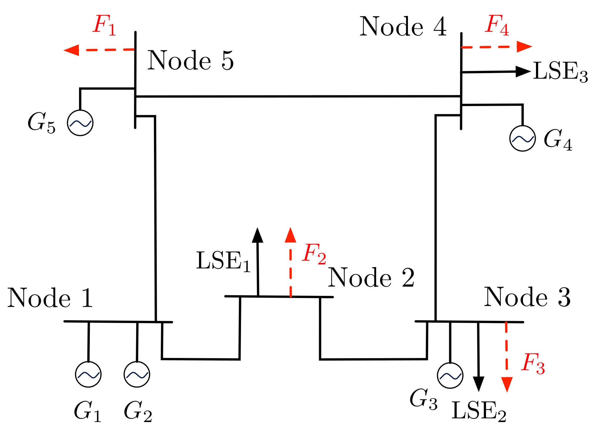
To validate the proposed framework we need to construct a power system with many voltage levels that will represent the transmission and distribution systems. As such, we select a five-node transmission system on which four distribution system feeders are connected to different nodes as depicted in Figure 2.

We denote by $F_i$ the ith feeder connected to the transmission system. More specifically, $F_1$ and $F_3$ correspond to the IEEE standard 33-bus feeder and $F_2$ and $F_4$ to the 69-bus IEEE standard bus feeder [44,45,46]. The load serving entities at a transmission node i are denoted by ${\mathrm{LSE}}_i$. There are five generators connected at the transmission level in nodes 1, 3, 4 and 5. 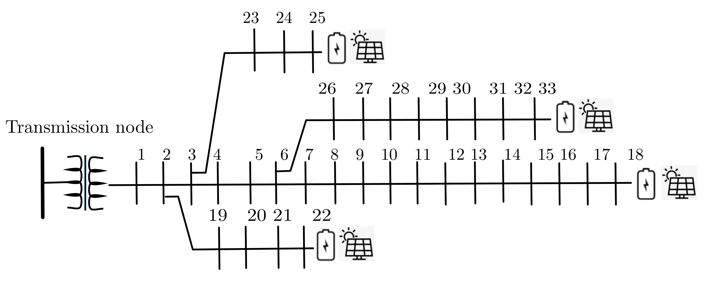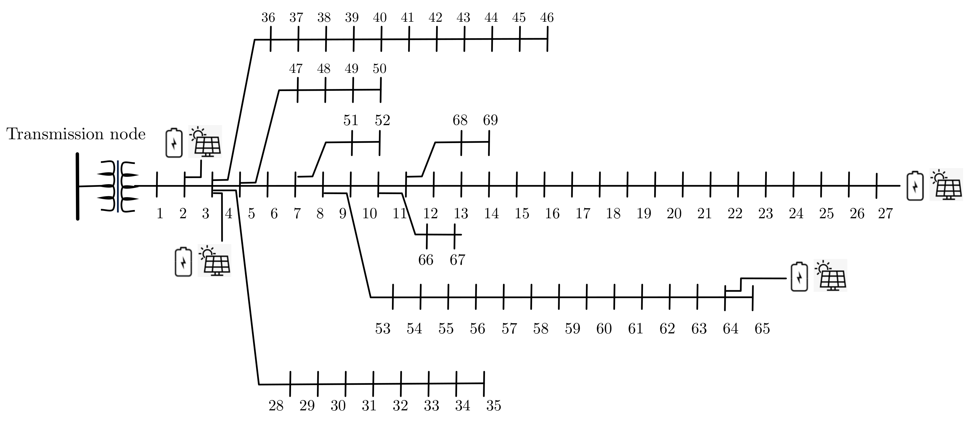The transmission system data may be found in [24]. To demonstrate how the TSO-DSO coordination schemes can facilitate the integration of DG we modify the standard IEEE 33- and 69-bus feeders by deploying PV and battery systems at different nodes. We assume that the distributed resources are mostly installed at end-nodes in the distribution level where the voltage drop levels are worst [47]. The modified feeders are depicted in Figure 3 and Figure 4, respectively. In particular, PV and battery systems are installed in nodes 18, 22, 25 and 33 in the 33-bus feeder and in nodes 2, 3, 27, and 64 in the IEEE 69-bus feeder. The distributed resources data are presented in

Table 1. Distributed resources’ physical limits and bid information.

Feeder	Variable	Value	Unit
All	$P_{PV}^{min}$	0	MW
All	$P_{PV}^{max}$	30	MW
All	$B_{PV}$	2.584	€/MW
$F_1$, $F_3$	$P_B^{\mathrm{dis},min}$	0	MW
$F_1$, $F_3$	$P_B^{\mathrm{dis},max}$	30	MW
$F_1$, $F_3$	$P_B^{\mathrm{ch},min}$	0	MW
$F_1$, $F_3$	$P_B^{\mathrm{ch},max}$	30	MW
$F_1$, $F_3$	$B_B^{\mathrm{dis},min}$	0.380	€/MW
$F_2$, $F_4$	$P_B^{\mathrm{dis},min}$	0	MW
$F_2$, $F_4$	$P_B^{\mathrm{dis},max}$	15	MW
$F_2$, $F_4$	$P_B^{\mathrm{ch},min}$	0	MW
$F_2$, $F_4$	$P_B^{\mathrm{ch},max}$	15	MW
$F_2$, $F_4$	$B_B^{\mathrm{dis},min}$	0.380	€/MW
$F_1$, $F_3$	$P_{\mathrm{grid}}^{min}$	–110	MW
$F_2$, $F_4$	$P_{\mathrm{grid}}^{min}$	–60	MW

. Furthermore, we assume that each node’s voltage in the distribution system is bounded between 0.95 $\mathrm{pu}$ and 1.05 $\mathrm{pu}$.

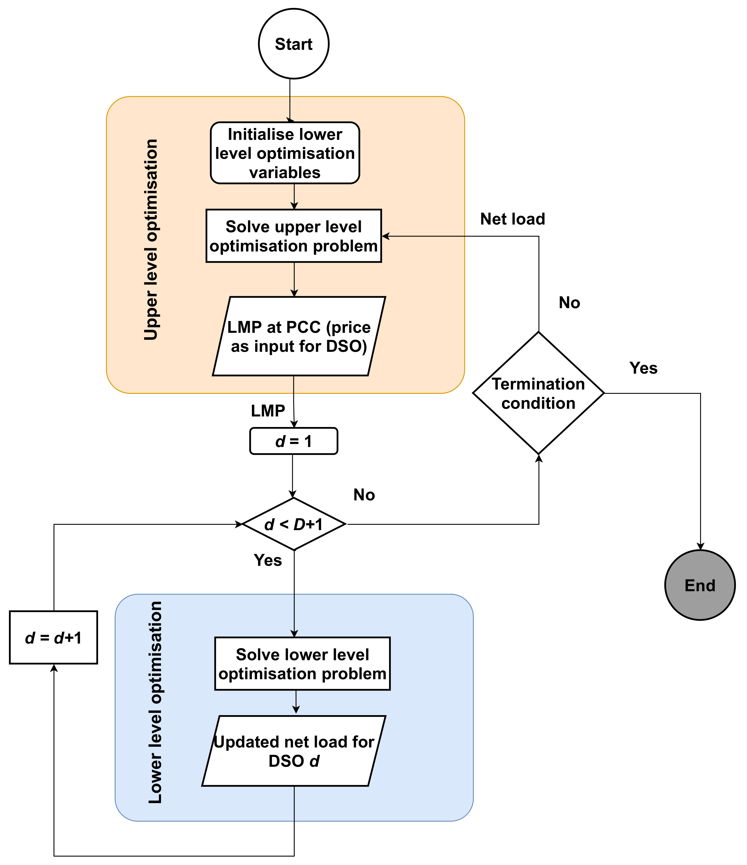
Next, we implement both the proposed centralised and the decentralised schemes, and we compare the results with current practise, which refers to when the TSO solves its OPF and determines the LMPs at the substations. Next, the DSOs dispatch distributed DG by optimising cost and considering the LMP at the substation as a fixed parameter. In current practise, there is minimal coordination between TSOs and DSOs. The three methodologies are compared against a variety of metrics: total cost, hourly LMPs, hourly DG output, hourly generator output at the transmission level, netload; and level of congestion.

4.2. Decentralised Coordination Scheme

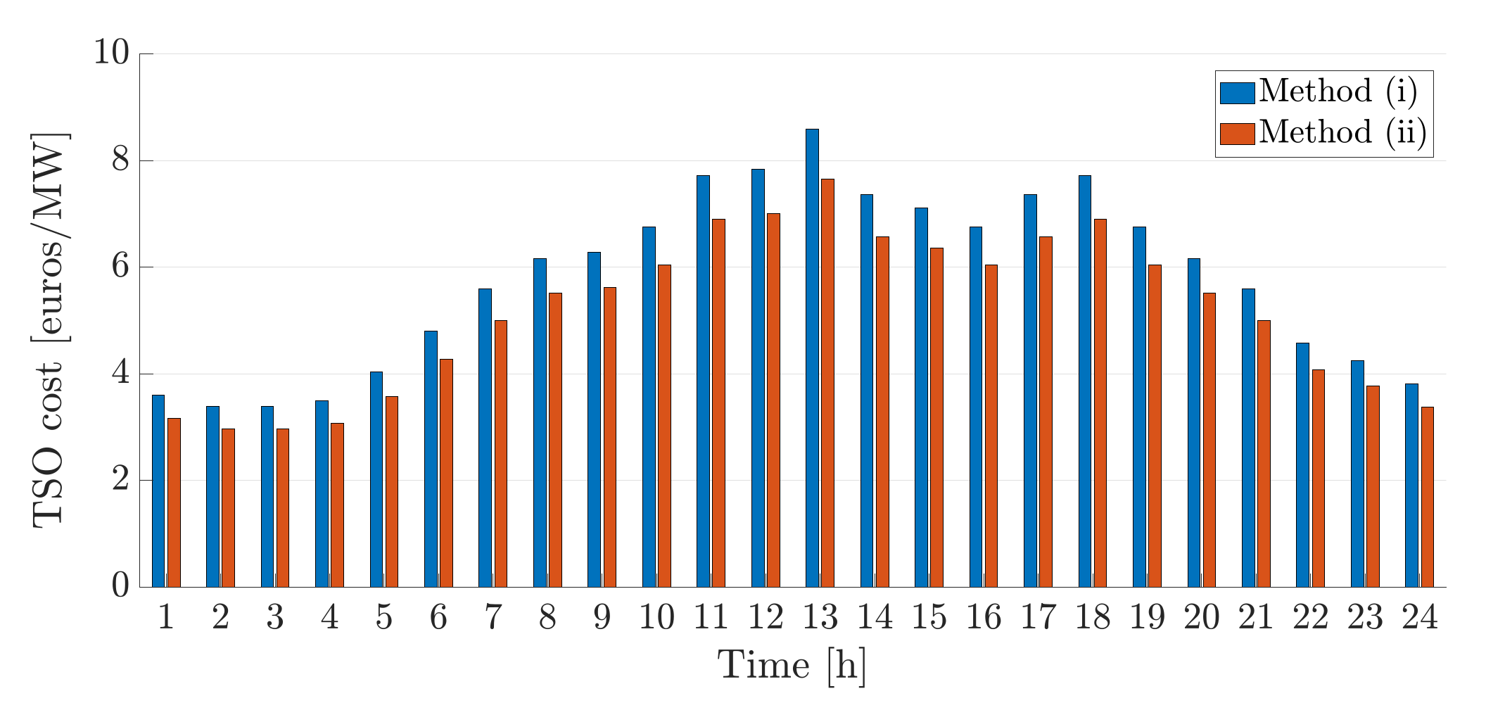
We apply the scheme proposed in Section 3.1 to the system described above. In order to demonstrate how the decentralised scheme facilitates the integration of distributed energy resources we compare its optimal operation (method (ii)) against current practice (method (i)), where the current practise as discussed in the introduction section is when the TSO solves its own OPF and determines the LMPs at the substation, and the DSOs dispatch DG by optimising cost and considering the LMP at the substation as a fixed parameter. We run both cases for a one day period with hourly intervals. 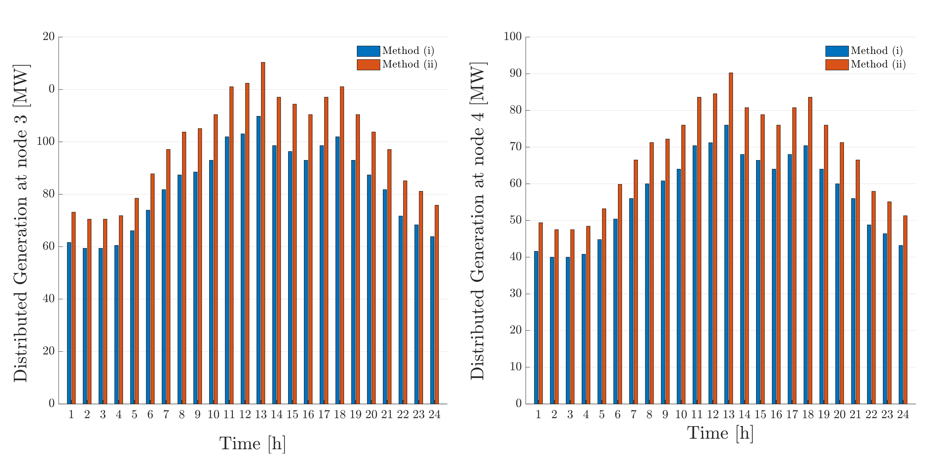In Figure 5, the TSO operation cost for both cases is depicted. We notice that the proposed decentralised coordination scheme results in a reduced transmission operation cost for all hours of the day. The reason is that distributed energy resources, which are less expensive than generators connected at the transmission level, are used to a greater extent as seen in Figure 6.

Another effect of the increasing use of distributed resources is that they relieve the congestion that is present in the transmission system, which in turn reduces TSO operational costs. For method (i) the LMPs for each hour at each node may be found in

Table 2. Locational marginal prices for method (i): current practise for TSO-DSO coordination in €/MW.

Hour	Node 1	Node 2	Node 3	Node 4	Node 5
1	12.67	28.15	25.22	17.15	13.46
2	12.62	28.01	25.10	17.08	13.41
3	12.62	28.01	25.10	17.08	13.41
4	12.64	28.08	25.16	17.11	13.44
5	12.76	28.42	25.45	17.30	13.56
6	12.93	28.89	25.87	17.55	13.74
7	13.09	29.36	26.28	17.80	13.92
8	13.21	29.70	26.58	17.99	14.05
9	13.23	29.77	26.64	18.02	14.08
10	13.32	30.04	26.88	18.17	14.18
11	13.51	30.58	27.35	18.46	14.39
12	13.53	30.65	27.41	18.49	14.41
13	13.68	31.05	27.76	18.71	14.57
14	13.44	30.38	27.17	18.35	14.31
15	13.39	30.24	27.05	18.28	14.26
16	13.32	30.04	26.88	18.17	14.18
17	13.44	30.38	27.17	18.35	14.31
18	13.51	30.58	27.35	18.46	14.39
19	13.32	30.04	26.88	18.17	14.18
20	13.21	29.70	26.58	17.99	14.05
21	13.09	29.36	26.28	17.80	13.92
22	12.88	28.75	25.75	17.48	13.69
23	12.81	28.55	25.57	17.37	13.62
24	12.71	28.28	25.34	17.22	13.51

. We notice that for the same hour each node has a different LMP. This demonstrates, based on the formulation of the augmented DCOPF in (1), that some line flows have reached their limits. The LMPs of method (ii) are shown in

Table 3. Locational marginal prices for method (ii): proposed decentralised TSO-DSO coordination in €/MW.

Hour	Node 1	Node 2	Node 3	Node 4	Node 5
1	12.27	12.28	12.28	12.27	12.27
2	12.13	12.14	12.14	12.14	12.13
3	12.13	12.14	12.14	12.14	12.13
4	12.20	12.21	12.21	12.21	12.20
5	12.54	12.55	12.55	12.54	12.54
6	13.01	13.02	13.02	13.01	13.01
7	12.55	28.14	25.19	17.06	13.35
8	12.88	12.89	12.89	12.88	12.88
9	12.90	12.91	12.91	12.90	12.90
10	12.98	12.99	12.99	12.99	12.98
11	13.15	13.16	13.16	13.15	13.15
12	13.17	13.18	13.18	13.17	13.17
13	11.93	11.94	11.94	11.94	11.93
14	13.08	13.10	13.10	13.09	13.08
15	13.04	13.06	13.06	13.05	13.04
16	12.98	12.99	12.99	12.99	12.98
17	13.08	13.10	13.10	13.09	13.08
18	13.15	13.16	13.16	13.15	13.15
19	12.98	12.99	12.99	12.99	12.98
20	12.88	12.89	12.89	12.88	12.88
21	12.55	28.14	25.19	17.06	13.35
22	12.87	12.89	12.89	12.88	12.87
23	12.67	12.68	12.68	12.68	12.67
24	12.40	12.41	12.41	12.41	12.40

. We notice that the LMP difference between hours has been reduced, reflecting the fact that there is less congestion in the transmission system. In fact the LMPs are practically the same for all nodes at every hour when the proposed decentralised scheme is implemented. Following the formulation of (1) and using the KKT conditions of optimality, the LMP difference is expressed as a function of the congestion that can be present in the network (see, e.g., in [48]), i.e.,:

$${\lambda }_k-{\lambda }_{k^{\prime }}=\sum _{\ell \in \tilde{\mathcal{L}}}{\varphi }_{\ell }^{\{k,k^{\prime }\}}{\mu }_{\ell },$$

(29)

where ${\mu }_{\ell }$ is the dual variable of the power flow limits for line ℓ; $\tilde{\mathcal{L}}$ is the subset of lines that are at their limits, i.e., $\tilde{\mathcal{L}}=\{{\ell }_i:i=1,\cdots ,L,{\mu }_{{\ell }_i}\ne 0\}$; and ${\varphi }_{\ell }^{\{k,k^{\prime }\}}$ is the power transfer distribution factor of transaction with node pair $\{k,k^{\prime }\}$ with respect to line ℓ. We can interpret (29) physically by considering an injection at node k and its withdrawal at node $k^{\prime }$. We interpret ${\varphi }_{\ell }^{\{k,k^{\prime }\}}$ as the fraction of the transaction with node pair $\{k,k^{\prime }\}$ of 1 MW that flows on line ℓ. As such for every hour the LMP differences are purely a function of the transmission usage costs of the congested lines, thus showing the “level” of congestion.

In

Table 4. The power output in MW of generators at the transmission level for method (i): current practise for TSO-DSO coordination.

Hour	${\mathit{P}}_{{\mathit{G}}_1}$	${\mathit{P}}_{{\mathit{G}}_2}$	${\mathit{P}}_{{\mathit{G}}_3}$	${\mathit{P}}_{{\mathit{G}}_4}$	${\mathit{P}}_{{\mathit{G}}_5}$
1	110	18.53	19.52	0	110
2	110	15.09	13.36	0	110
3	110	15.09	13.36	0	110
4	110	16.81	16.44	0	110
5	110	25.41	31.84	0	110
6	110	37.45	53.39	0	110
7	110	49.5	74.95	0	110
8	110	58.1	90.35	0	88.4
9	110	59.82	93.43	0	90.88
10	110	60	110	2.45	100.81
11	110	43.78	110	57.07	110
12	94.58	60.36	110.71	60	110
13	62.8	0.03	116.72	42.99	110
14	110	55.25	110	31.2	110
15	110	60	110	16.85	108.26
16	110	60	110	2.45	100.81
17	110	55.25	110	31.2	110
18	110	43.78	110	57.07	110
19	110	60	110	2.45	100.81
20	110	58.1	90.35	0	88.4
21	110	49.5	74.95	0	110
22	110	34.01	47.23	0	110
23	110	28.85	38	0	110
24	110	21.97	25.68	0	110

and

Table 5. The power output in MW of generators at the transmission level for method (ii): proposed decentralised TSO-DSO coordination.

Hour	${\mathit{P}}_{{\mathit{G}}_1}$	${\mathit{P}}_{{\mathit{G}}_2}$	${\mathit{P}}_{{\mathit{G}}_3}$	${\mathit{P}}_{{\mathit{G}}_4}$	${\mathit{P}}_{{\mathit{G}}_5}$
1	39.14	0	0	0	110
2	30.02	0	0	0	110
3	30.02	0	0	0	110
4	34.58	0	0	0	110
5	57.38	0	0	0	110
6	89.3	0	0	0	110
7	107.99	6.66	6.58	0	110
8	82.98	0	0	0	88.4
9	85.82	0	0	0	90.88
10	91.19	0	0	0	100.81
11	101.05	0.88	0	0	110
12	101.78	1.49	0	0	110
13	9.58	0	0	0	110
14	97.9	0	0	0	110
15	95.22	0	0	0	108.26
16	91.19	0	0	0	100.81
17	97.9	0	0	0	110
18	101.05	0.88	0	0	110
19	91.19	0	0	0	100.81
20	82.98	0	0	0	88.4
21	107.99	6.66	6.58	0	110
22	80.18	0	0	0	110
23	66.5	0	0	0	110
24	48.26	0	0	0	110

the hourly power output of each transmission generator is shown. We notice that with method (ii) the total power used by generators at the transmission level is reduced compared to method (i). The reason is that the less expensive distributed generators at distribution level are used to satisfy the load instead. More specifically, we notice that with method (ii) the transmission level generators 2, 3, and 4 have zero output for most hours of the day as they are the most expensive ones.

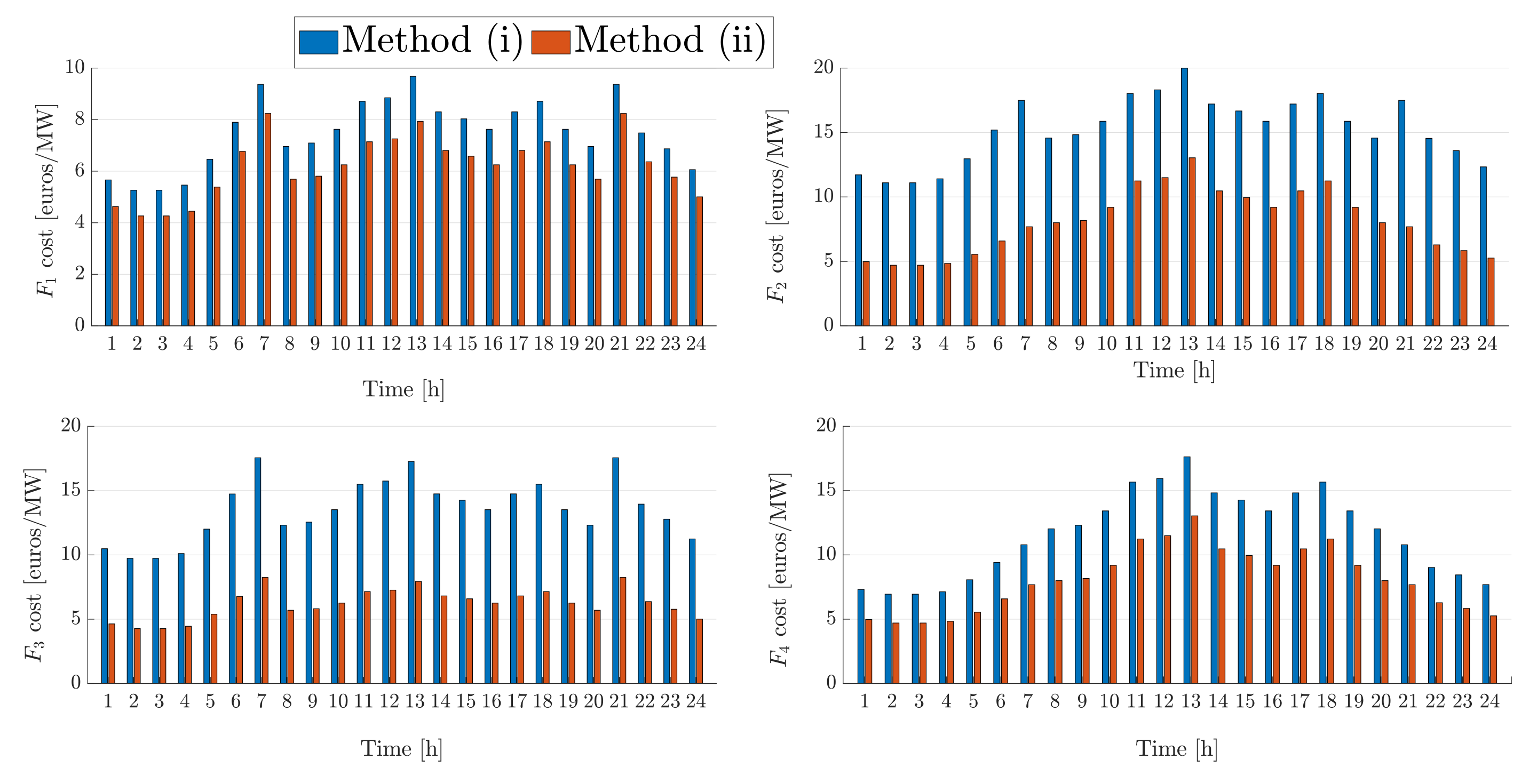
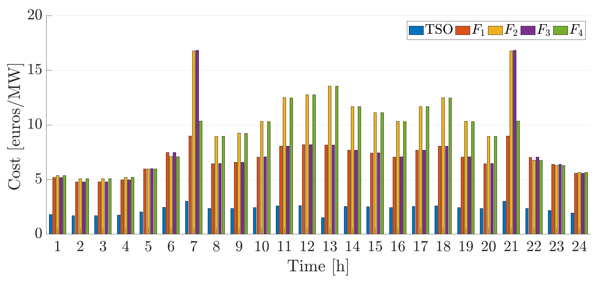
In Figure 7 we depict the operational cost for each distribution feeder connected to different nodes of the transmission system for methods (i) and (ii). We notice that the proposed coordination scheme results in reduced costs for all DSOs as all resources were utilised in a more efficient way as discussed above.

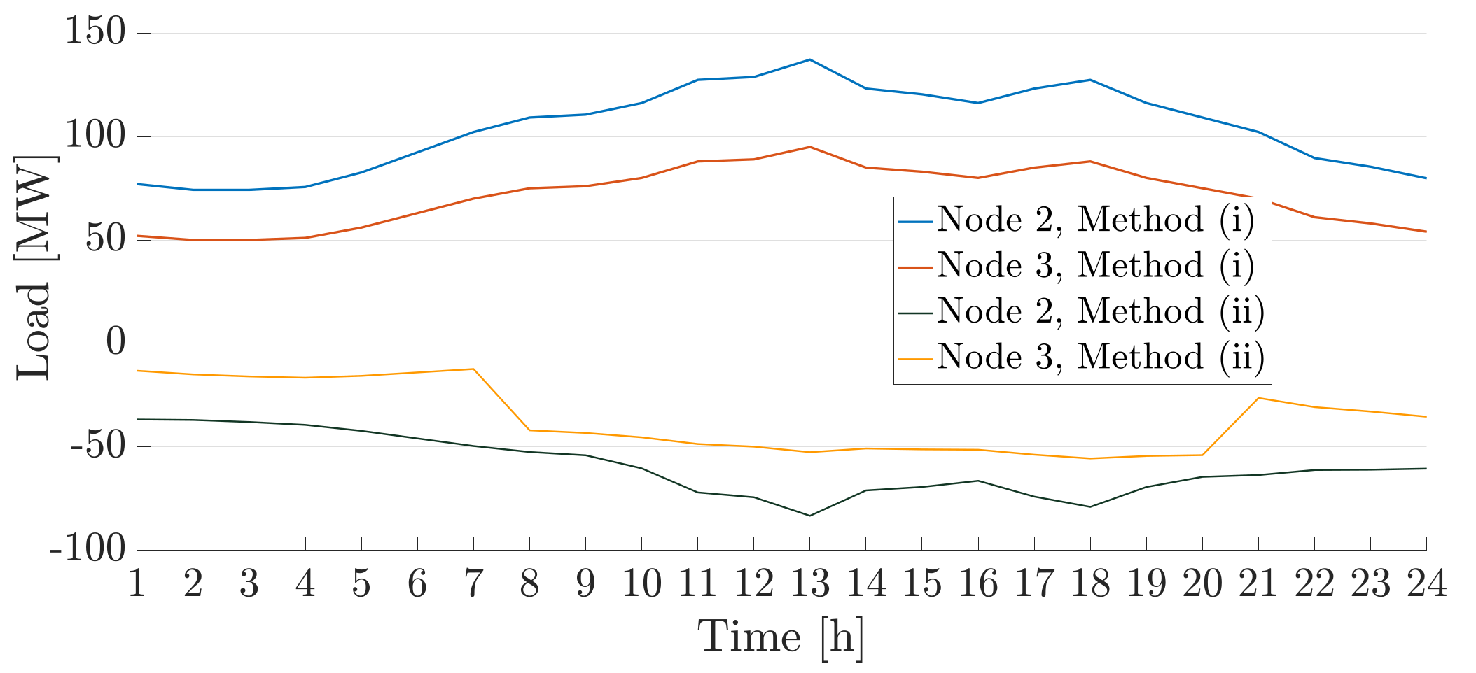
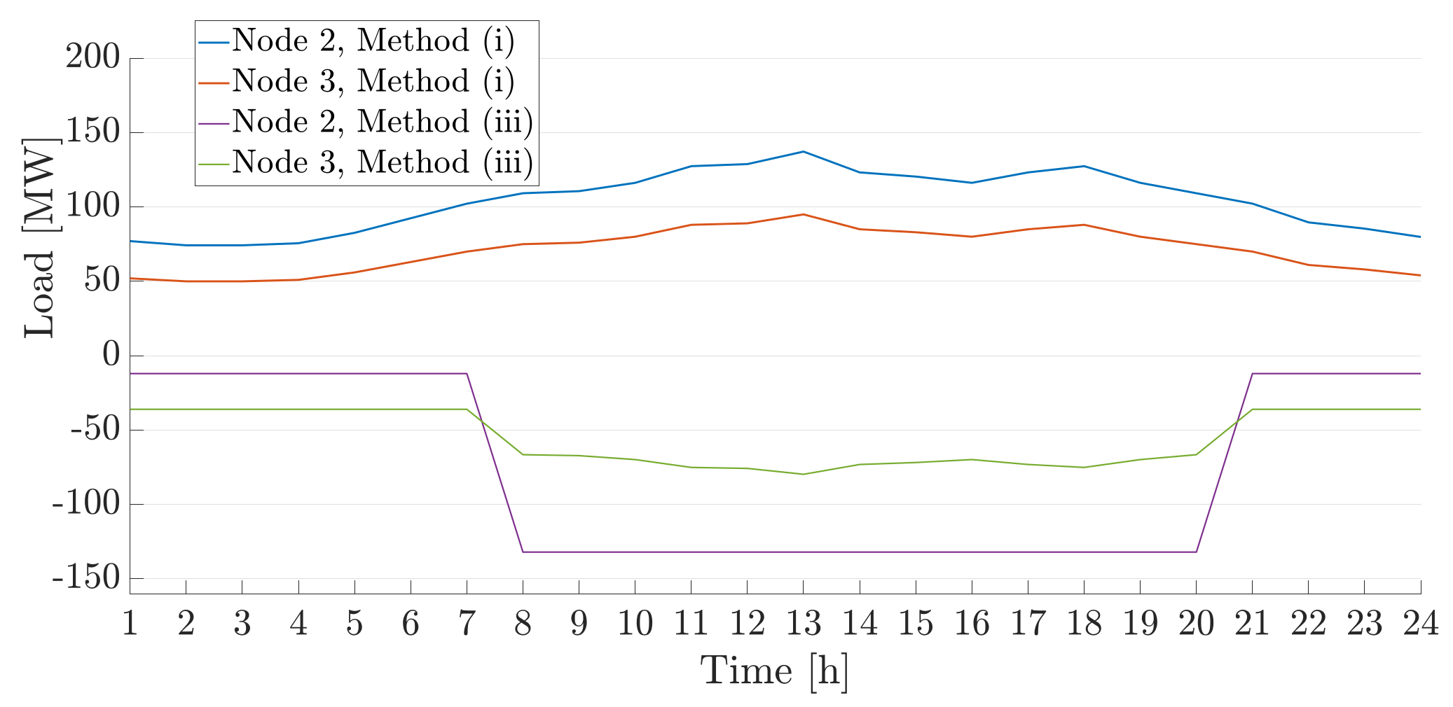
We now study the net load at the transmission nodes using both methods. We can see in Figure 8 that the net loads at the transmission system at nodes 2 and 3 decrease, a fact that is also reflected in the OPF in the transmission system and its LMPs. We also notice that there is a sharp fall and rise in the net load, between hours 7 and 8 and 20 and 21 respectively. This is due to the fact that the power flow between nodes 1 and 2 at time 7 and 21 is 75 MW, which is equal to the line’s thermal limit. This causes the LMP divergence in these hours, as shown in Table 3.

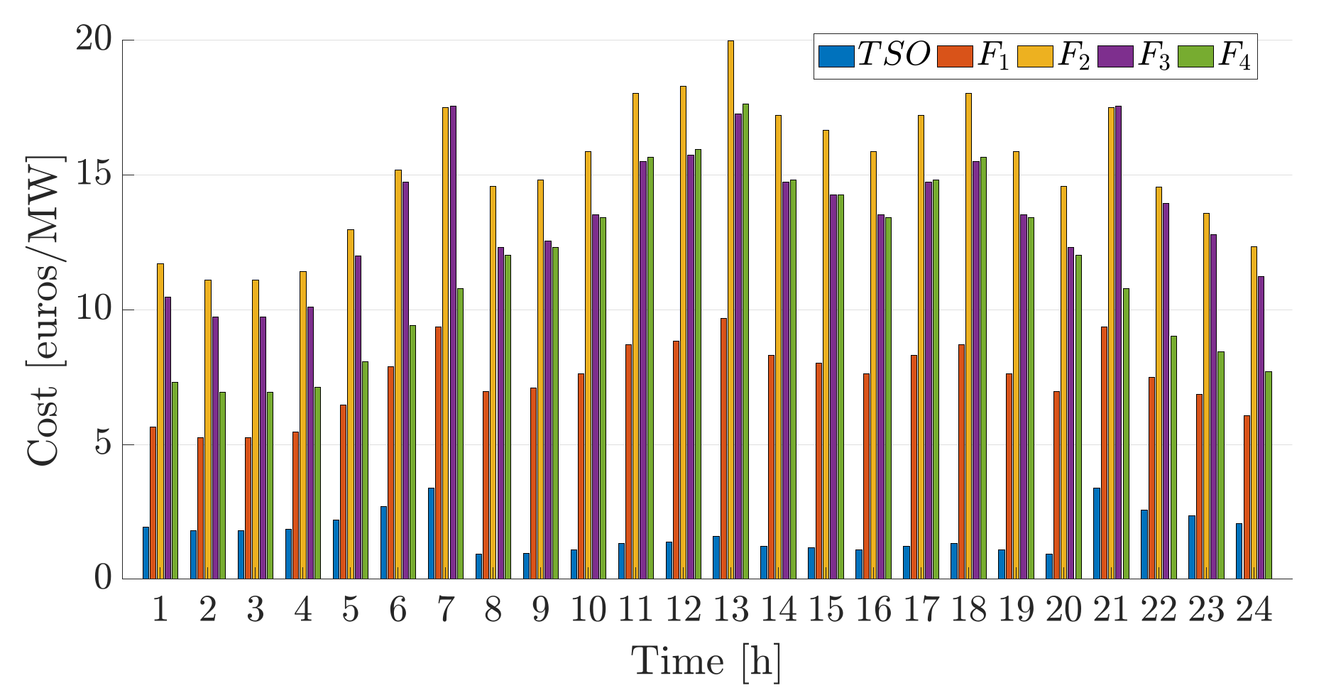
Last, we depict the hourly operational cost for the TSO and the DSOs in Figure 9 which will be used to compare the two proposed schemes.

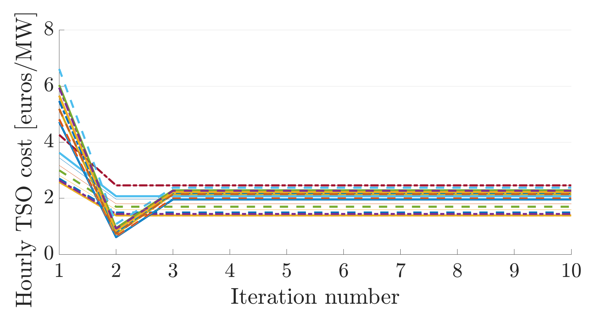
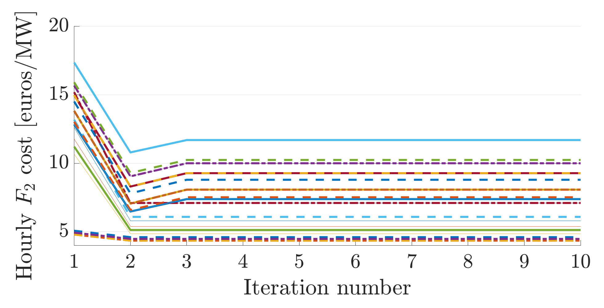
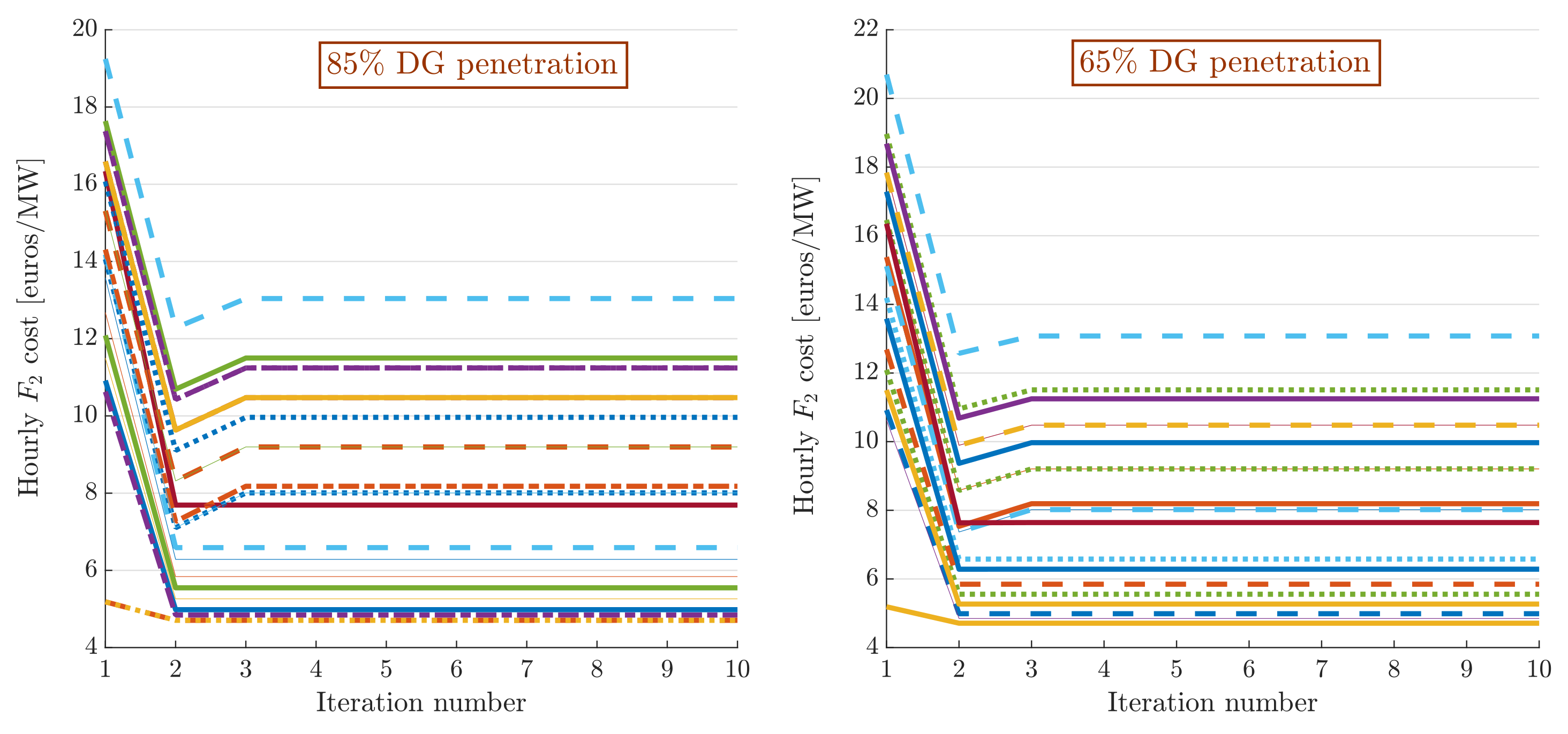
We next check the convergence properties of the proposed algorithm. In Figure 10 and Figure 11 we illustrate the evolution of the hourly objective functions of $F_2$ and the transmission system for a 24-h period with respect to the iteration numbers of algorithm. We notice that the algorithm converges after three iterations. To test the sensitivity of the proposed algorithm with respect to the initial point, i.e., the choice of initial load value for the distribution system, we changed the initial point to be full load, 85%, 75%, and 65% of the full load. In all cases the algorithm converges in three iterations. Next, to analyse the sensitivity of the proposed algorithm with respect to the level of distributed resources penetration we depict in Figure 12 the evolution of $F_2$ hourly cost for two different levels of penetration with the same initial point (step 3 of the algorithm) with respect to the number of iterations. The final cost is different for the two cases since there are hours where the DG price is smaller than the grid price and vice versa.

4.3. Centralised Coordination Scheme

We apply the proposed scheme developed in Section 3.2 to the system described in Figure 2. In order to demonstrate how the proposed centralised scheme can facilitate the integration of distributed energy resources we compare method (i), which is the optimal operation with the current practise, with method (iii), which is the proposed centralised scheme. We start the simulation by assigning the same weights to the transmission cost function and the distribution feeders’ cost functions as $w_1=w_2=0.5$. 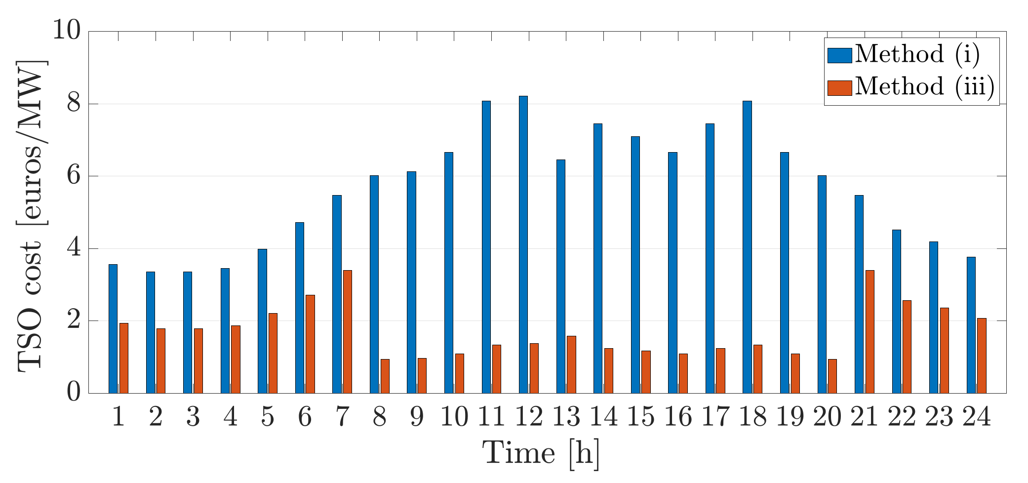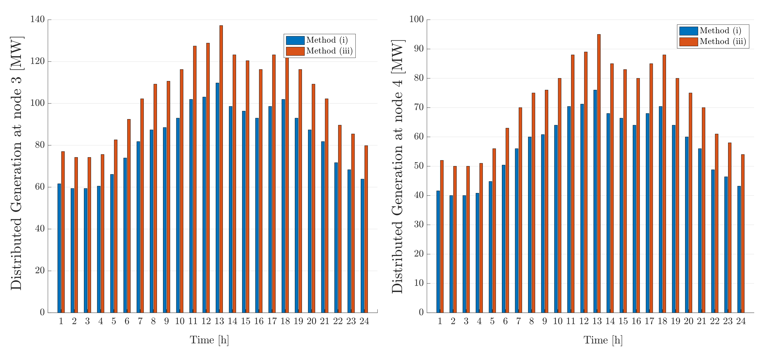The TSO cost as depicted in Figure 13 is reduced significantly with method (iii), i.e., the centralised scheme, in comparison to the current practise due to the increase in the integration of the distributed resources at different nodes as shown in Figure 14.

In Figure 15 the net load at the transmission level using methods (i) and (iii) is depicted. We notice that it is more cost efficient for the TSO to purchase power from the DG that is present in the distribution systems. For instance, the negative load at node 2 means that the excess power of the distributed resources is redirected to the transmission system. DGs usually sell at a price equal to the LMP at their PCC. This results in distributed resources’ owners gaining revenue by selling power to the TSO, while the TSO also meets its load at a lower cost. In Figure 16 the operational cost for each hour for the TSO and DSOs for the proposed centralised coordination scheme is depicted. Figure 16 shows that the transmission cost for method (iii) with $w_1=w_2=0.5$ is lower than that of method (ii) as depicted in Figure 9. The difference is that more power is being used from the DGs in method (iii) compared to that of method (ii). However, we notice that the cost of feeders in method (iii) is higher than that of method (ii). Again, this is due to the fact that more power is being used from the DGs in method (iii) compared to that of method (ii). These values can be used by DSOs and TSOs to formulate their bids and provide incentives for DG participation respectively.

The hourly power output of transmission generators for method (iii) is presented in

Table 6. The power output in MW of generators at the transmission level for method (iii): proposed centralised TSO-DSO coordination.

Hour	${\mathit{P}}_{{\mathit{G}}_1}$	${\mathit{P}}_{{\mathit{G}}_2}$	${\mathit{P}}_{{\mathit{G}}_3}$	${\mathit{P}}_{{\mathit{G}}_4}$	${\mathit{P}}_{{\mathit{G}}_5}$
1	52.05	0	0	0	110
2	42.45	0	0	0	110
3	42.45	0	0	0	110
4	47.25	0	0	0	110
5	71.25	0	0	0	110
6	102.64	2.2	0	0	110
7	110	10.87	17.58	0	110
8	0	0	0	0	88.4
9	0	0	0	0	90.88
10	0	0	0	0	100.81
11	10.67	0	0	0	110
12	13.15	0	0	0	110
13	28.05	0	0	0	110
14	3.22	0	0	0	110
15	0	0	0	0	108.26
16	0	0	0	0	100.81
17	3.22	0	0	0	110
18	10.67	0	0	0	110
19	0	0	0	0	100.81
20	0	0	0	0	88.4
21	110	10.87	17.58	0	110
22	95.25	0	0	0	110
23	80.85	0	0	0	110
24	61.65	0	0	0	110

. We notice that between hours 8 and 20 the distributed resources located in the distribution systems satisfy the load at the transmission level, whereas at night hours mostly the TSO is responsible for supplying the load to the customers. This reverse power flow also impacts the LMP as shown in

Table 7. Locational marginal prices for method (iii): proposed centralised TSO-DSO coordination in €/MW.

Hour	Node 1	Node 2	Node 3	Node 4	Node 5
1	14.52	14.53	14.53	14.53	14.52
2	14.42	14.43	14.43	14.43	14.42
3	14.42	14.43	14.43	14.43	14.42
4	14.47	14.48	14.48	14.48	14.47
5	14.71	14.72	14.72	14.72	14.71
6	15.03	15.04	15.04	15.03	15.03
7	15.13	27.74	25.35	18.78	15.78
8	11.24	11.24	11.24	11.24	11.24
9	11.27	11.27	11.27	11.27	11.27
10	11.41	11.41	11.41	11.41	11.41
11	14.11	14.11	14.11	14.11	14.11
12	14.13	14.13	14.14	14.13	14.13
13	14.28	14.28	14.29	14.28	14.28
14	14.03	14.03	14.04	14.04	14.03
15	11.52	11.52	11.52	11.52	11.52
16	11.41	11.41	11.41	11.41	11.41
17	14.03	14.03	14.04	14.04	14.03
18	14.11	14.11	14.11	14.11	14.11
19	11.41	11.41	11.41	11.41	11.41
20	11.24	11.24	11.24	11.24	11.24
21	15.13	27.74	25.35	18.78	15.78
22	14.95	14.97	14.97	14.96	14.95
23	14.81	14.82	14.82	14.81	14.81
24	14.62	14.63	14.63	14.62	14.62

, where we notice a marginal increase in the LMPs for the night hours is achieved. Similar to method (ii) there is congestion at hours 7 and 21 due to the congested line between nodes 1 and 2.

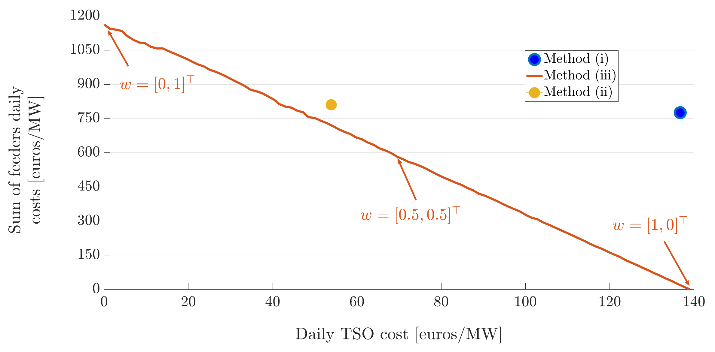
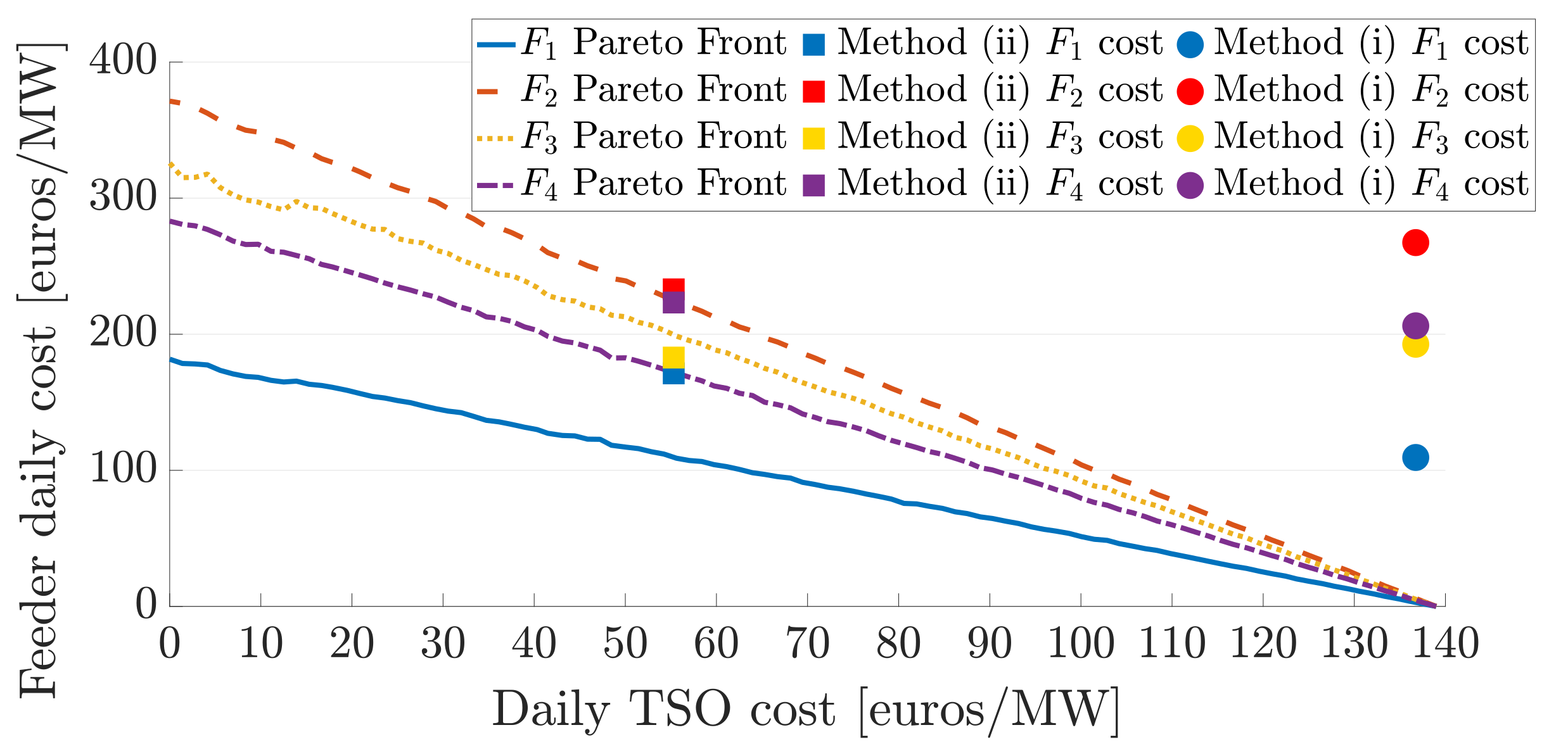
Next, we analyse the interaction between the TSO and the DSOs. For this, we modify the weights of (28) to obtain an approximation of the Pareto front. More specifically, we start with $w_1=0$ and $w_2=1$, and with increments of $0.05$ we reach $w_1=1$ and $w_2=0$. The Pareto front is depicted in Figure 17. By moving along the curve, we can minimise DSOs’ objective at the expense of TSO’s objective, or minimise the TSO’s objective at the expense of DSOs’ objective. However we cannot improve both at once, i.e., there is no mathematical “best” point along the Pareto front.

To provide insights into the potential conflicts between TSOs and DSOs we discuss in greater detail the two extreme cases, i.e., $w_1=0$ and $w_2=1$ and $w_1=1$ and $w_2=0$. The TSO and DSO costs for the first one are 0 €/MW and 500 €/MW, respectively; and for the latter they are 140 €/MW and 0 €/MW, respectively. In other words, when the objective is to only minimise the TSO cost; all costs are being incurred by the DSOs and vice versa. In both cases, all constraints, e.g., voltage and thermal limits, are met thus the power system quality is guaranteed.

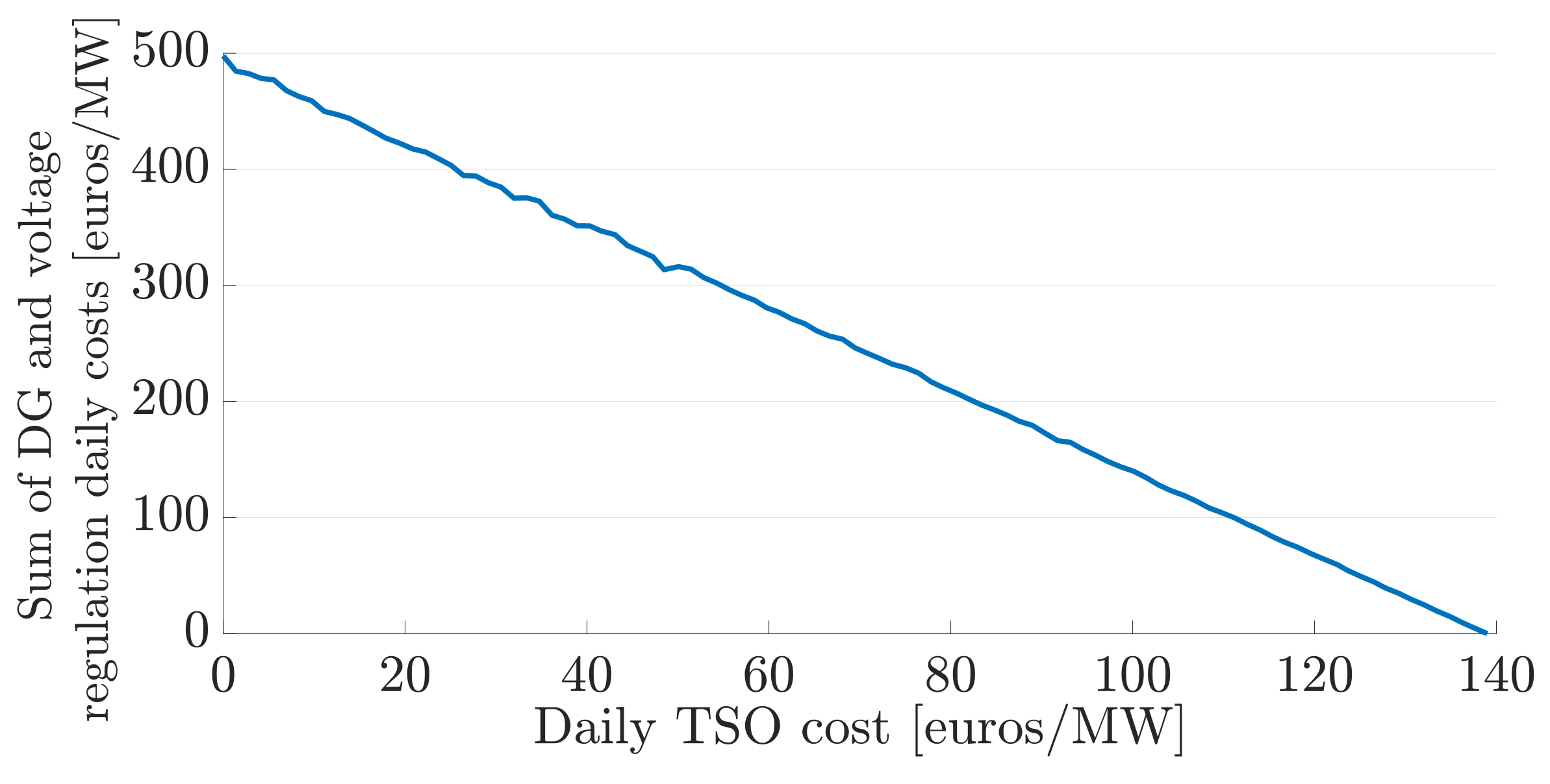
In Figure 18, we depict the total DSO cost that includes the payments to the TSO given in (9), DG cost given in (10) and (11), and voltage regulation costs given in (12). We compare the results for different weights with methods (i) and (ii). We notice that the results of method (ii) are close to the Pareto front offering a near-optimal solution. The appropriate choice of operation for the Pareto front is a balance of priorities between TSOs and DSOs and the determination of specific incentives, which are part of future work. Another implication of the Pareto front is that any point in the feasible region that is not on the Pareto front is not considered to be a “good” solution, e.g., method (i). Either objective, or both, can be improved at no penalty to the other. This demonstrates that there are a lot of improvements to be made to current TSO-DSO coordination practise, i.e., method (i). To determine the priorities of the proposed decentralised scheme, we have to analyse where its solution lies in the Pareto front. More specifically, we notice in Figure 18 and Figure 19 that the proposed decentralised scheme provides a balance between the TSO and DSO objective, as it lies between the two extreme cases.

Next, we depict in Figure 19 the daily cost of individual feeders, which includes the payments to the TSO, the cost of DG and voltage regulation, to investigate how far from the optimal solution each feeder operates for the various schemes. We notice that for method (ii), $F_2$ operates at the optimum, $F_3$ at a point that is at the expense of other feeders, and $F_1$ and $F_4$ at points further away from the optimal solutions. However, the summation of these costs corresponds to a near optimal solution as seen in Figure 18.

In both schemes, the transmission cost decreases, while for method (iii), the transmission operation cost reduction is higher than that of method (ii). In comparison to the current practise, i.e., method (i), both schemes are more effective in terms of the share contribution of the distributed generators at each transmission node, while the utilisation rate of generation for method (iii) is higher than that of method (ii). Using method (iii), we can see that the output of each generator at the transmission level is lower than that of method (ii) and for method (ii) is lower than that of method (i). Although for method (ii) and method (iii), the congestion level is improved, the LMP for each node at each hour is higher at night hours in method (iii). This is due to the increased output of transmission generators at night hours. It should be noted that in all case studies all variables, e.g., voltage levels, transmission line flows, are kept within the limits of acceptable for power quality purposes as defined by the constraints of the OPFs. For example, voltage levels of each bus in the distribution system at every time interval are in the range of 0.95–1.05 pu. The algorithm running time for the centralised scheme is 12,387 ms and for the decentralised is 21,800 ms in a Windows machine which is equipped with AMD^® FX-9830P RADEON R7 CPU with four Cores at 3.00 GHz and 16 GB of RAM. As expected the centralised scheme is approximately two times faster; however both schemes are fast enough for real-time operation purposes.

5. Conclusions and Discussion

In this paper, we have presented a novel TSO-DSO coordination framework that increases the efficient use of distributed generation resources. More specifically, we have two coordination schemes: one centralised, another decentralised. The underlying network for both systems is approximated linearly and the OPF formulations result in convex optimisation problems. We have formulated a decentralised TSO-DSO coordination scheme based on an iterative approach where no sensitive information is exchanged that achieves a near-optimal solution. Next, we analysed the interaction of TSOs and DSOs and how conflicting their objectives are by approximating the Pareto front of a multi-objective OPF problem where the entire system, i.e., transmission and distribution systems, is modelled. Through numerical results we have demonstrated that both coordination schemes result in (i) reduced operational costs for both TSOs and DSOs, (ii) congestion relief, and (iii) increased use of distributed generation.

In the two proposed schemes, different entities are responsible for making a decision and, thus, diverse information is shared between them. In particular, in the centralised scheme the TSO makes the decisions and has access to all information about the underlying physical distribution systems as well as DG bidding. In the decentralised scheme, both the DSO and TSO share the decision-making-process and the only information that the TSO sends the DSO is the LMP at the PCC and the DSO to the TSO its net load. The two proposed methods also differ in the total cost, level of DG integration, voltage levels and level of congestion, as demonstrated in the numerical results’ section. These affect the “power quality” of the system. However, all variables, e.g., voltage levels, and transmission line flows, are kept within the limits of acceptable for power quality purposes as defined by the constraints of the OPFs.

There are natural extensions of the work presented here. For instance, a distributed solution of the proposed centralised scheme is necessary so that system operators do not share sensitive information about their topology and generators bids. Moreover, a more detailed representation on the topology of the distribution system would provide more accurate results as well as incorporation of uncertainty in renewable-based generation. We will report on these developments in future papers.

References

1. Gerard, H.; Rivero Puente, E.I.; Six, D. Coordination between transmission and distribution system operators in the electricity sector: A conceptual framework. Util. Policy 2018, 50, 40–48. [Google Scholar] [CrossRef]
2. Caramanis, M.C.; Goldis, E.; Ruiz, P.A.; Rudkevich, A. Power market reform in the presence of flexible schedulable distributed loads. New bid rules, equilibrium and tractability issues. In Proceedings of the 2012 50th Annual Allerton Conference on Communication, Control, and Computing (Allerton), Monticello, IL, USA, 1–5 October 2012; pp. 1089–1096. [Google Scholar] [CrossRef]
3. Najibi, F.; Apostolopoulou, D.; Alonso, E. Enhanced performance Gaussian process regression for probabilistic short-term solar output forecast. Int. J. Electr. Power Energy Syst. 2021, 130, 106916. [Google Scholar] [CrossRef]
4. Najibi, F.; Alonso, E.; Apostolopoulou, D. Optimal Dispatch of Pumped Storage Hydro Cascade under Uncertainty. In Proceedings of the IEEE 2018 UKACC 12th International Conference on Control (CONTROL), Sheffield, UK, 5–7 September 2018; pp. 187–192. [Google Scholar]
5. Kärkkäinen, S. Integration of demand-side management, distributed generation, renewable energy sources and energy storages. In Proceedings of the CIRED 2012 Workshop: Integration of Renewables into the Distribution Grid, Lisbon, Portugal, 29–30 May 2008; Volume 1, p. 77. [Google Scholar]
6. De Jong, G.; Franz, O.; Hermans, P.; Lallemand, M. TSO-DSO Data Management Report; TSO-DSO Project Team: ENTSO-E, CEDEC, GEODE, EURELECTRIC and EDSO; ENTSO-E: Brussels, Belgium, 2016. [Google Scholar]
7. Yuan, Z.; Hesamzadeh, M.R. Hierarchical coordination of TSO-DSO economic dispatch considering large-scale integration of distributed energy resources. Appl. Energy 2017, 195, 600–615. [Google Scholar] [CrossRef]
8. Hadush, S.Y.; Meeus, L. DSO-TSO cooperation issues and solutions for distribution grid congestion management. Energy Policy 2018, 120, 610–621. [Google Scholar] [CrossRef] [Green Version]
9. Birk, M.; Chaves-Ávila, J.P.; Gómez, T.; Tabors, R. TSO/DSO coordination in a context of distributed energy resource penetration. In Proceedings of the EEIC, MIT Energy Initiative Reports, Cambridge, MA, USA, 17 October 2017; pp. 2–3. [Google Scholar]
10. Najibi, F.; Niknam, T.; Kavousi-Fard, A. Optimal stochastic management of renewable MG (micro-grids) considering electro-thermal model of PV (photovoltaic). Energy 2016, 97, 444–459. [Google Scholar] [CrossRef]
11. Najibi, F.; Niknam, T. Stochastic scheduling of renewable micro-grids considering photovoltaic source uncertainties. Energy Convers. Manag. 2015, 98, 484–499. [Google Scholar] [CrossRef]
12. Ashouri, A.; Sels, P.; Leclercq, G.; Devolder, O.; Geth, F.; D’hulst, R. Smart TSO-DSO Interaction Schemes, Market Architectures, and ICT Solutions for the Integration of Ancillary Services from Demand-Side Management and Distributed Generation Network and Market Models; EU Report, SmartNet, April 2017. Available online: https://cordis.europa.eu/project/id/691405 (accessed on 29 June 2021).
13. Givisiez, A.G.; Petrou, K.; Ochoa, L.F. A Review on TSO-DSO Coordination Models and Solution Techniques. Electr. Power Syst. Res. 2020, 189, 106659. [Google Scholar] [CrossRef]
14. Merino, J.; Gómez, I.; Turienzo, E.; Madina, C.; Cobelo, I.; Morch, A.; Saele, H.; Verpoorten, K.; Puente, E.; Häninnen, S.; et al. Ancillary service provision by RES and DSM connected at distribution level in the future power system. SmartNet Proj. D 2016, 1, 1. [Google Scholar]
15. Kristov, L.; De Martini, P.; Taft, J.D. A Tale of Two Visions: Designing a Decentralized Transactive Electric System. IEEE Power Energy Mag. 2016, 14, 63–69. [Google Scholar] [CrossRef]
16. Savvopoulos, N.; Konstantinou, T.; Hatziargyriou, N. TSO-DSO coordination in decentralized ancillary services markets. In Proceedings of the IEEE 2019 International Conference on Smart Energy Systems and Technologies (SEST), Porto, Portugal, 9–11 September 2019; pp. 1–6. [Google Scholar]
17. Dempe, S.; Kalashnikov, V.; Pérez-Valdés, G.A.; Kalashnykova, N. Bilevel programming problems. In Energy Systems; Springer: Berlin, Germany, 2015. [Google Scholar]
18. Papavasiliou, A. Analysis of distribution locational marginal prices. IEEE Trans. Smart Grid 2017, 9, 4872–4882. [Google Scholar] [CrossRef] [Green Version]
19. Sorin, E.; Bobo, L.; Pinson, P. Consensus-based approach to peer-to-peer electricity markets with product differentiation. IEEE Trans. Power Syst. 2018, 34, 994–1004. [Google Scholar] [CrossRef] [Green Version]
20. Papavasiliou, A.; Mezghani, I. Coordination Schemes for the Integration of Transmission and Distribution System Operations. In Proceedings of the 2018 Power Systems Computation Conference (PSCC), Dublin, Ireland, 11–15 June 2018; pp. 1–7. [Google Scholar] [CrossRef]
21. Saint-Pierre, A.; Mancarella, P. Active Distribution System Management: A Dual-Horizon Scheduling Framework for DSO/TSO Interface Under Uncertainty. IEEE Trans. Smart Grid 2017, 8, 2186–2197. [Google Scholar] [CrossRef]
22. Huang, S.; Wu, Q.; Oren, S.S.; Li, R.; Liu, Z. Distribution Locational Marginal Pricing Through Quadratic Programming for Congestion Management in Distribution Networks. IEEE Trans. Power Syst. 2015, 30, 2170–2178. [Google Scholar] [CrossRef] [Green Version]
23. Rossi, M.; Migliavacca, G.; Viganò, G.; Siface, D.; Madina, C.; Gomez, I.; Kockar, I.; Morch, A. TSO-DSO coordination to acquire services from distribution grids: Simulations, cost-benefit analysis and regulatory conclusions from the SmartNet project. Electr. Power Syst. Res. 2020, 189, 106700. [Google Scholar] [CrossRef]
24. Sun, J.; Tesfatsion, L.; Goldfarb, D.; Hogan, W.; Kirschen, D.; Liu, C.C.; Mccalley, J.; Powell, M.J.D.; Price, J.; Salazar, H.; et al. DC Optimal Power Flow Formulation and Solution Using QuadProgJ. In Iowa State University Digital Repository, Economics Working Papers (2002–2016), 253; Iowa State University Digital Repository: Ames, IA, USA, 2010. [Google Scholar]
25. Zhu, H.; Liu, H.J. Fast local voltage control under the limited reactive power: Optimality and stability analysis. IEEE Trans Power Syst. 2016, 31, 3794–3803. [Google Scholar] [CrossRef]
26. Franco, J.F.; Ochoa, L.F.; Romero, R. AC OPF for smart distribution networks: An efficient and robust quadratic approach. IEEE Trans. Smart Grid 2017, 9, 4613–4623. [Google Scholar] [CrossRef] [Green Version]
27. Montoya, O.D.; Gil-González, W.; Garces, A. Optimal Power Flow on DC Microgrids: A Quadratic Convex Approximation. IEEE Trans. Circuits Syst. II Express Briefs 2019, 66, 1018–1022. [Google Scholar] [CrossRef]
28. Ochoa, L.N.; Pilo, F.; Keane, A.; Cuffe, P.; Pisano, G. Embracing an Adaptable, Flexible Posture: Ensuring That Future European Distribution Networks Are Ready for More Active Roles. IEEE Power Energy Mag. 2016, 14, 16–28. [Google Scholar] [CrossRef]
29. Arnold, D.B.; Sankur, M.D.; Negrete-Pincetic, M.; Callaway, D.S. Model-Free Optimal Coordination of Distributed Energy Resources for Provisioning Transmission-Level Services. IEEE Trans. Power Syst. 2018, 33, 817–828. [Google Scholar] [CrossRef]
30. Vicente-Pastor, A.; Nieto-Martin, J.; Bunn, D.W.; Laur, A. Evaluation of Flexibility Markets for Retailer–DSO–TSO Coordination. IEEE Trans. Power Syst. 2019, 34, 2003–2012. [Google Scholar] [CrossRef]
31. Yang, R.; Hao, J.; Jiang, H.; Jin, X. Machine-Learning-Driven, Site-Specific Weather Forecasting for Grid-Interactive Efficient Buildings; Technical Report; National Renewable Energy Lab. (NREL): Golden, CO, USA, 2020. [Google Scholar]
32. Krechel, T.; Sanchez, F.; Gonzalez-Longatt, F.; Chamorro, H.; Rueda, J.L. Chapter 11—Transmission system-friendly microgrids: An option to provide ancillary services. In Distributed Energy Resources in Microgrids; Chauhan, R.K., Chauhan, K., Eds.; Academic Press: New York, NY, USA, 2019; pp. 291–321. [Google Scholar] [CrossRef]
33. Energy Networks Association. Open Networks Project: Opening Markets for Network Flexibility; Energy Networks Association: London, UK, 2017. [Google Scholar]
34. Caramanis, M.; Ntakou, E.; Hogan, W.W.; Chakrabortty, A.; Schoene, J. Co-Optimization of Power and Reserves in Dynamic T D Power Markets With Nondispatchable Renewable Generation and Distributed Energy Resources. Proc. IEEE 2016, 104, 807–836. [Google Scholar] [CrossRef]
35. West, D.B. Introduction to Graph Theory; Orentice Hall: Upper Saddle River, NJ, USA, 2001. [Google Scholar]
36. Morstyn, T.; Teytelboym, A.; Hepburn, C.; McCulloch, M.D. Integrating P2P Energy Trading with Probabilistic Distribution Locational Marginal Pricing. IEEE Trans. Smart Grid 2019. [Google Scholar] [CrossRef]
37. Bylling, H.C. Bilevel Optimization with Application in Energy. Ph.D. Thesis, Department of Mathematical, Faculty of Science, University of Copenhagen, Copenhagen, Denmark, 2018. [Google Scholar]
38. Von Stackelberg, H. Market Structure and Equilibrium; Springer: Berlin/Heidelberg, Germany, 1934. [Google Scholar]
39. Audet, C.; Hansen, P.; Jaumard, B.; Savard, G. Links between linear bilevel and mixed 0–1 programming problems. J. Optim. Theory Appl. 1997, 93, 273–300. [Google Scholar] [CrossRef]
40. Sinha, A.; Soun, T.; Deb, K. Using Karush-Kuhn-Tucker proximity measure for solving bilevel optimization problems. Swarm Evol. Comput. 2019, 44, 496–510. [Google Scholar] [CrossRef]
41. Britzelmeier, A.; De Marchi, A.; Gerdts, M. An Iterative Solution Approach for a Bi-level Optimization Problem for Congestion Avoidance on Road Networks. In Numerical Methods for Optimal Control Problems; Springer International Publishing: Cham, Switzerland, 2018; pp. 23–38. [Google Scholar] [CrossRef]
42. Cohon, J. Multiobjective Programming and Planning; Academic Press: New York, NY, USA, 1978. [Google Scholar]
43. Shan, S.; Wang, G.G. An Efficient Pareto Set Identification Approach for Multiobjective Optimization on Black-Box Functions. J. Mech. Des. 2004, 127, 866–874. [Google Scholar] [CrossRef] [Green Version]
44. Vardani, B. Optimum Location of SVC in an IEEE 33 Bus Radial Distribution System Using Power Sensitivity Index. In Proceedings of the 2019 International Conference on Electrical, Electronics and Computer Engineering (UPCON), Aligarh, India, 8–10 November 2019; pp. 1–5. [Google Scholar] [CrossRef]
45. Savier, J.S.; Das, D. Impact of Network Reconfiguration on Loss Allocation of Radial Distribution Systems. IEEE Trans. Power Deliv. 2007, 22, 2473–2480. [Google Scholar] [CrossRef]
46. Baran, M.; Wu, F. Network reconfiguration in distribution systems for loss reduction and load balancing. IEEE Trans. Power Deliv. 1989, 4, 1401–1407. [Google Scholar] [CrossRef]
47. Sadiq, A.; Adamu, S.; Buhari, M. Optimal distributed generation planning in distribution networks: A comparison of transmission network models with FACTS. Eng. Sci. Technol. Int. J. 2019, 22, 33–46. [Google Scholar] [CrossRef]
48. Apostolopoulou, D.; Gross, G.; Güler, T. Optimized FTR Portfolio Construction Based on the Identification of Congested Network Elements. IEEE Trans. Power Syst. 2013, 28, 4968–4978. [Google Scholar] [CrossRef]
Figure 1. Decentralised iterative scheme flowchart.
Sustainability 13 07832 g001
Figure 2. Transmission and distribution system.
Sustainability 13 07832 g002
Figure 3. Modified IEEE 33-bus distribution feeder.
Sustainability 13 07832 g003
Figure 4. Modified IEEE 69-bus distribution feeder.
Sustainability 13 07832 g004
Figure 5. Transmission operation cost for methods (i) current practise and (ii) proposed decentralised TSO-DSO coordination scheme.
Sustainability 13 07832 g005
Figure 6. The total amount of distributed generation for methods (i) current practise and (ii) proposed decentralised TSO-DSO coordination scheme at nodes 3 and 4.
Sustainability 13 07832 g006
Figure 7. The cost for each feeder for methods (i) and (ii).
Sustainability 13 07832 g007
Figure 8. Netload at nodes 2,3 with using methods (i) and (ii).
Sustainability 13 07832 g008
Figure 9. TSO and DSOs operational cost using the proposed decentralised coordination scheme.
Sustainability 13 07832 g009
Figure 10. Evolution of the hourly cost for F 2 with respect to the iteration number.
Sustainability 13 07832 g010
Figure 11. Evolution of the hourly cost for the transmission system with respect to the iteration number.
Sustainability 13 07832 g011
Figure 12. Evolution of hourly cost for F 2 for different penetration levels of distributed generation.
Sustainability 13 07832 g012
Figure 13. Transmission operation cost for methods (i) current practise and (iii) proposed centralised TSO-DSO coordination scheme.
Sustainability 13 07832 g013
Figure 14. The total amount of distributed generation for methods (i) current practise and (iii) proposed centralised TSO-DSO coordination scheme at nodes 3 and 4.
Sustainability 13 07832 g014
Figure 15. Net load at nodes 2, and 3 with using methods (i) and (iii).
Sustainability 13 07832 g015
Figure 16. TSO and DSOs operational cost using the proposed centralised coordination scheme.
Sustainability 13 07832 g016
Figure 17. Pareto Front of the sum of all feeders DG and voltage regulation daily cost with respect to the TSO cost.
Sustainability 13 07832 g017
Figure 18. Pareto Front of the sum of all feeders daily cost with respect to the TSO cost.
Sustainability 13 07832 g018
Figure 19. Pareto Front of daily cost for F i , i = 1 , , 4 with respect to the TSO cost.
Sustainability 13 07832 g019