Abstract
Seismic fragility analysis is an efficient method to evaluate the structural failure probability during earthquake events. Among the existing fragility analysis methods, the probabilistic seismic demand model (PSDM) and the joint probabilistic seismic demand model (JPSDM) are generally used to compute the component and system fragility, respectively. However, the statistical significance behind the parameters related to the current PSDM and JPSDM are not comparable. Aside from that, when calculating the system fragility, the Monte Carlo sampling (MCS) method is time-consuming. To solve the two flaws, in this paper, the logarithm piecewise functions were used to generate the PSDM and the JPSDM, and the MCS was replaced by the univariate conditioning approximation (UCA) method. The concepts and application procedures of the proposed fragility analysis methods were elaborated first. Then, the UCA method was illustrated in detail. Finally, fragility curves of a steel arch truss case study bridge were generated by the proposed method. The research results indicate the following: (1) the proposed methods unify the data sources and statistical significance of the parameters used in the PSDM and the JPSDM; (2) the logarithmic piecewise function-based PSDM sensitively reflects the changing trend of the component’s demand with the fluctuation of the seismic intensity measure; (3) under transverse seismic waves, major injuries happen on the side bearings of the bridge, while slight damage may occur on each pier, and as the seismic intensity measure increases, the side bearings are more likely to be damaged; (4) for the severe damage and the absolute damage of the studied bridge, the system fragility curves are closer to the upper failure bounds; and (5) compared with the MSC method, the accuracy of the UCA method can be guaranteed with less calculation time.
1. Introduction
Since the Pacific Earthquake Engineering Research Center (PEER) proposed performance-based earthquake engineering (PBEE), seismic fragility analysis has been widely promoted and applied in earthquake-resistant structures [1,2,3,4,5,6]. So far, seismic fragility analysis has mainly adopted the empirical method and the theoretical method [7,8]. The empirical method is limited in use because its data come from real earthquakes [9], while the theoretical method is user-friendly and widely used in structural seismic risk assessment because it is based on the structural finite element model, whose data are controllable [10,11,12,13,14]. Aside from that, with the development of deep learning, many artificial intelligence methods [15,16,17] have been applied to civil engineering [18,19,20,21] and related seismic fragility evaluation [22,23,24].
In the theoretical method, to consider the uncertainties of the ground motion and the structure, the probabilistic seismic demand model (PSDM) is generally used. Meanwhile, Cornell et al. [10] first assumed that both the structural demand and the structural capacity obey the log-normal distribution. Based on the above assumption, many scholars conducted seismic fragility analysis on different types of bridges. For example, Li et al. [25] investigated the seismic fragility of a typical multi-span reinforced concrete continuous girder bridge experiencing chloride ion-induced corrosion. They concluded that non-uniform chloride-induced corrosion may change the vulnerable position and damage mechanisms of RC columns. Zakeri et al. [7] discussed how the skew angle influenced the seismic fragility of the skewed single-frame, concrete, box-girder bridges. Different component responses were studied. Their calculation results revealed that older bridges are particularly susceptible to column damage and are not sensitive to skew. Zhong et al. [26] generated seismic fragility curves of a cable-stayed bridge using various spatial variables. The results indicated that the section ductility demands at the base of the pylon are significantly affected by the spatial variabilities of the ground motion. Wu et al. [27] developed both the component and system fragility curves of a concrete cable-stayed bridge. This research concluded that the fragility functions are sensitive to the stiffness of the cable restrainer, and the longitudinal constraint system performs better than the totally floating system and the totally rigid system. Yılmaz et al. [28] studied the seismic fragility of a railway truss bridge with tension capacity as the damage index (DI) of the load-carrying ability and lateral displacement as the DI of serviceability. The results showed that the velocity limit of this bridge must be reduced. Herath et al. [29] studied how soft soil conditions influenced the distribution of peak ground accelerations (PGAs), and the results were informative when generating the PSDM.
It is noteworthy that current seismic fragility analysis mainly focuses on the main components of the bridge. In other words, the fragility of the pier or the main tower is used to represent the fragility of the whole bridge. However, the damage to other components like the deck, cable, and abutment will affect the performance of the bridge too. For example, a falling beam would occur if the support displacement exceeds the limitation. Additionally, the bridge must be closed for maintenance if the cable is broken. All these conditions will cause traffic interruption and economic losses. Seismic fragility analysis is the major foundation of performance-based seismic design (PBSD). One purpose of this analysis is to conduct risk assessment for the whole structure; therefore, it is very important to obtain not only the component fragility curves but also the system fragility curves.
The calculation of system fragility is a sophisticated reliability problem. In structural reliability theory, when calculating the system failure, there are three types of systems: series systems, parallel systems, and mixed systems. It is obvious that the parallel system is not appropriate for bridge structures because the failure of its main component will lead to the whole bridge failing (e.g., piles or main towers), and this is against the definition of the parallel system. The mixed system highly corresponds with reality. However, bridges have many components, and how these components influence the responses of the whole bridge has not been clearly studied yet. Therefore, the difficulty of establishing a convincing mixed system model leads to the mixed system rarely being used. In the series system, components are connected in a single-chain order, and thus this system is easier to establish and more conservative than the mixed system. By the two advantages, the series system is generally used when computing the system fragility of bridges [30,31,32,33,34,35,36,37,38,39,40,41,42].
Among the existing system fragility methods, the first-order or second-order reliability method is commonly used due to their simple structures [30,31,32,33]. Chen [30] calculated the system fragilities of several tall-pier bridges subjected to near-fault ground motions by the first-order reliability method. Wu et al. [31] evaluated the system vulnerability of a high-pier long-span bridge with the same method. Pan et al. [32] and Gao et al. [33] obtained the system fragilities of girder bridges by the second-order reliability method. However, these two methods can only determine the lower and upper failure bounds, rather than specify an exact failure curve. The reason for this is that the above methods make very strong assumptions about the correlation of different components’ responses which are different from reality. In order to determine the exact failure curve, Qin et al. [34] established the limit state function of a contemporary house when it was subjected to wind uplift and calculated the system fragility by the Monte Carlo Sampling (MCS) method. Mangalathu et al. [35] used the lasso logistic regression technique to derive the multi-dimensional system fragility function of skewed concrete bridge classes. Zhou et al. [36] established the system response model by copula functions with different copulas and conducted the system failure assessment of a typical seismically isolated reinforced concrete (RC) frame structure. Xu et al. [37] proposed a multi-variate, non-stationary random field theory to determine the system fragility of a transportation system while considering six different deterioration levels.
Aside from the methods mentioned above, a group of scholars represented by Nielson [38], Wang et al. [39], and Wu et al. [27,31] directly extended the component level fragility to the system level fragility by proposing the joint probabilistic seismic demand model (JPSDM). The JPSDM originates from the PSDM, and compared with other methods, there are two advantages to apply the JPSDM: (1) the calculation process of the system fragility curves becomes very similar to that of the component fragility ones, and (2) conceptually, the calculation of the component fragility and system fragility forms a closed loop. Therefore, the JPSDMs were generated and the system fragility curves were calculated by some scholars [40,41,42]. Nevertheless, there are still two flaws of the current JPSDM: (1) although the PSDM and the JPSDM are merged into a single system conceptually, when conducting the calculations, the JPSDM ignores the statistical significances behind parameters related to the PSDM, which means the two models cannot be merged into a general system mathematically, and (2) when calculating the system fragility after the JPSDM is generated, the generally used MCS method is time-consuming.
In this paper, to merge the PSDM and JPSDM conceptually and mathematically and to reduce the system fragility calculation time, component and related system fragility analysis methods using a logarithmic piecewise function were proposed, and the MSC method was replaced by an alternative method. A steel truss arch bridge was used as an example to illustrate the calculation process, and its transverse component and system fragility curves were generated. More specifically, by fitting the PSDM and the JPSDM with a logarithmic piecewise function, the corresponding parameters of the PSDM and JPSDM are matched. Simultaneously, the traditional MCS method is replaced by the univariate conditional approximation (UCA) method to improve the computational efficiency. The traditional and proposed fragility analysis methods are introduced in Section 2 and Section 3, respectively. In Section 4, how to apply the UCA method is illustrated. In Section 5, the modeling details of the studied bridges, the used seismic waves, and the damage indexes are described. In Section 6, the transverse components and system fragility curves are generated and analyzed. Section 7 is the conclusions.
2. The Traditional Fragility Analysis Methods
2.1. The Component Fragility Analysis Method
According to the classical reliability analysis theory, structure fragility is described as the conditional probability under a given ground motion intensity. The following formula can be established according to the definition:
where Pf is the conditional probability of failure, Sd is the structural seismic demand, and Sc is the structural seismic capacity. Sd and Sc are assumed to follow the log-normal distribution. Equation (1) can be rewritten as follows:
because
where λ is the mean and β is the standard deviation of the normal distribution.
It is known that
where Φ is the standard normal cumulative distribution function and and are the predicted (i.e., the conditional median) values of the seismic demand and capacity, respectively.
In the PSDM, the monitored engineering demand parameter (EDP) is combined with the corresponding intensity measure (IM) to build the power PSDM [10]:
where a and b are the estimated parameters from the linear regression analysis. To account for the uncertainties of the PSDM, the dispersion (standard deviation) of the seismic demand (βd) is calculated by the following formula:
where Di is the ith realization of the structural demand and n is the number of the used ground motions.
Figure 1 shows the components PSDM generated by the cloud approach [43] and the incremental dynamic analysis (IDA) method [44].
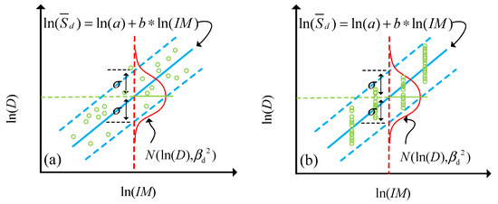
Figure 1.
The PSDM based on (a) the cloud approach [43] and (b) the IDA method [44].
2.2. The System Fragility Analysis Method
2.2.1. System Fragility Analysis Based on the First-Order Reliability Method
The first-order reliability method assumes that once one of the components fails, the entire system fails (i.e., the series system). This method finds the upper and lower bounds of the system failure as show in Equation (10):
where Psys is the system failure probability and Pi is the failure probability of the ith component. This method makes very strong assumptions of the dependency among components. The lower bound treats components as completely related; that is, the failure of one component will trigger the failure of all other components. On the contrary, the upper bound regards each component as completely independent, and the failure of any component has no influence on the remaining ones.
2.2.2. System Fragility Analysis Based on the Joint Probabilistic Seismic Demand Model
Similarly, in a series system, the corresponding failure probability can be obtained by the Monte Carlo method if the joint probabilistic density functions (PDFs) of both the demand and the capacity are known. Figure 2 shows the joint PDF and related failure range (the shaded area) of a two-component system [40]. In this method, the dependencies among all components are determined by calculation and not by assumptions.
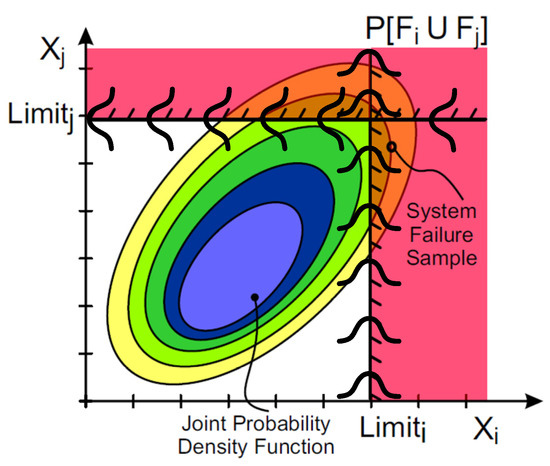
Figure 2.
The PDF of the demand and the related failure domain for a 2D case [40].
The principle of this method is as follows. For a system composed of n components, assume the system demand under a fixed ground motion intensity measure (IM) is X = (X1, X2…, Xn). If the PSDM of each component follows the log-normal distribution, each edge distribution of ln (X) should distribute normally (i.e., Yi = ln (Xi) follows the normal distribution). By calculating the correlation coefficients of all Yi and combining the response variance of all components, the covariance matrix of the demand can be set up. Aside from that, each element of the mean vector of the demand under a set IM can be obtained by Equation (8). With both the mean vector and the covariance matrix, the joint PDF of the demand (or the JPSDM) at a set IM is established [38].
The correlative coefficient is calculated by the following formula:
in which ρij is the element in the ith row and jth column of the correlation coefficient matrix, Cov[Yi,Yj] is the sample covariance of vector Yi, and Yj, D[Yi] represents the sample variance of vector Yi.
Theoretically, in the method proposed by Nielson [38], only one correlation coefficient matrix is used for all IMs, while in reality, with different ground motion IM, the response relationship between components will change, resulting in different correlation coefficient matrixes. In addition, statistically, the parameters of the correlation coefficient matrix do not match the parameters of the corresponding edge distribution if the correlation coefficient matrices under all IMs are represented by the correlation coefficient matrix under a certain IM. A detailed explanation is shown in the following paragraph. Assume that this system was composed of two components, and four seismic waves were inputted into the system accordingly (each seismic wave was amplified to three IM by the IDA method), using A and B to represent the component responses, and the same subscript suggests the responses under the same seismic wave as displayed in Figure 3.
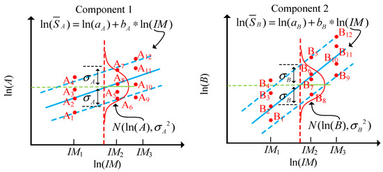
Figure 3.
The PSDM of a two-component system by the IDA method.
Suppose the data at IM1 are used to calculate the sample covariance matrix, whose diagonal elements are taken from Equation (12) as
in which
Similarly, data at IM2 or IM3 can also be used to generate the sample covariance matrix. However, since the diagonal elements of the correlation coefficient matrix are one, when calculating the covariance matrix by the variances of the correlation coefficient matrix and the marginal distributions, the corresponding diagonal elements are
It can be seen that the final results and physical meanings of Equations (12) and (14) are different. The results obtained from Equation (12) are sample variances of all responses of the components at a certain IM, while Equation (14) calculates the error variances of the regression function of the components.
In the traditionally used method [38], the covariance matrix (matrix one) and the correlation coefficient matrix (matrix two) are first calculated by Equation (11), and then a new covariance matrix (matrix three) is generated by combining the correlation coefficient matrix (matrix two) with the variances taken from Equation (14). In other words, the sample variances obtained from Equation (12) are replaced by the error variances of the regression function when generating the covariance matrix of the JPSDM. Such a replacement changes the statistical meaning of the original covariance matrix so that the newly used covariance matrix (matrix three) does not reflect the statistical significance of the original components’ responses, which is to say that this replacement does not match the traditional process of using a covariance matrix to calculate the failure probability and may cause calculation errors.
3. The Proposed Fragility Analysis Methods
In this section, a logarithmic piecewise function-based component and related system fragility analysis methods are proposed. The proposed methods could solve the problem of mismatch in statistical significances between the PSDM and JPSDM and improve the fitting accuracy of the PSDM.
3.1. The Component Fragility Analysis Method Based on the Logarithmic Piecewise Function
To solve the problem of a mismatch in statistical significances between the PSDM and JPSDM, the linear fitting function of the PSDM (Figure 1) needs to be replaced by a piecewise fitting function (Figure 4). The following paragraph illustrates the replacement process when the IDA method is used. It is worth noting that if not the IDA method, but the cloud approach is used, the seismic responses could also be transformed into the same format as shown in the literature [45], so the proposed method is still appliable.
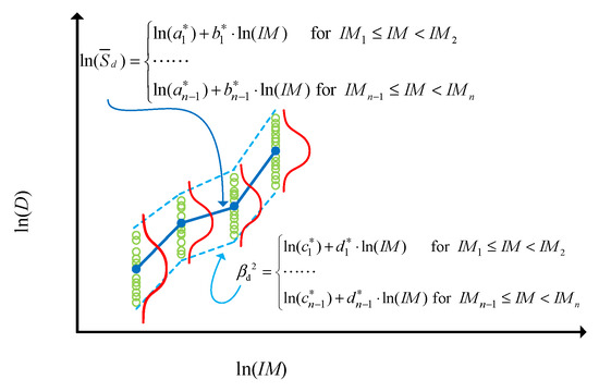
Figure 4.
The PSDM based on the logarithm piecewise function.
In Figure 1, the component demand in the whole IM domain followed a normal distribution with a linearly varying mean (in the whole logarithmic coordinate space) and a constant variance. If the mean and the variance were turned into values changing linearly with IM segments (not in the whole IM space but in different IM segments) as shown in Figure 4, the fitting accuracy and the sensitivity of the PSDM would be improved.
The specific steps are as follows:
Step 1. Transform the structural demands and the IM into the logarithmic coordinate space (so all parameters mentioned in Steps 2 and 3 are log coordinate-based).
Step 2. At each IM, calculate the mean and the sample variance of the demands.
Step 3. Use the linear interpolation to fit the calculated means and variances.
In accordance with the above statements, when calculating the fragility of the components, Equation (8) could be replaced by Equation (15) with
Equation (9) could be replaced by Equation (16) with
where , , , and (i = 1, 2, 3, …, n − 1) are the interpolation parameters, IMi (i = 1, 2, 3, …, n) is the breakpoint, and n − 1 is the number of segments for the piecewise linear interpolation.
3.2. The System Fragility Analysis Method Based on the Logarithmic Piecewise Function
The proposed system fragility analysis method is illustrated by a two-component system. First, generate the logarithmic piecewise function-based PSDM of each component as shown in Figure 5.
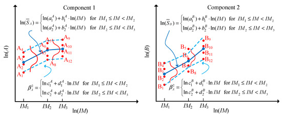
Figure 5.
The PSDM of the components using the logarithmic piecewise function.
Then, build the JPSDM at each IM. Take the moment of IM1 as an example. The mean vector of the joint distribution at this moment is , where
When calculating the covariance matrix and the correlation coefficient matrix of IM1, only A1–A4 and B1–B4 are used; that is, the diagonal elements of the covariance matrix are the same as the sample variances of the marginal distributions, as shown in Equation (18), and the error variances of the linear regression are not applied:
The above calculation process ensures that only one covariance matrix is used at IM1 (i.e., only using matrix one without using matrix three), so the statistical significances of the covariance matrix and the components’ responses can be guaranteed. At IM2 and IM3, the results can be obtained by the same method. For the JPSDM between IM1 and IM2 (or IM2 and IM3), the mean vectors are also computed by Equation (17), and the non-diagonal elements of the correlation coefficient matrix are obtained by linear interpolation between and (the diagonal elements of the correlation coefficient matrix are always one). Therefore, with the mean vectors, the variances of all components, and the correlation coefficient matrices, the joint distributions between IM2 and IM3 (or IM2 and IM3) can be determined.
In general, regardless of the variation of the seismic IM, a set of corresponding mean vectors and covariance matrices can always be found (i.e., the multivariate normal distribution describing the JPSDM can be determined for any seismic IM). As can be seen, the proposed method does not apply the regression error variances throughout the calculation, and the statistical significances behind the parameters related to the PSDM and the JPSDM are comparable.
4. The Univariate Conditioning Approximation Method
When calculating the system failure probability at different IMs using the method proposed in Section 3.2, there are infinite multivariate joint log-normal distributions for the demand. Thus, using the Monte Carlo sampling (MCS) method is computationally intensive. According to the additivity of the multivariate normal distribution, the univariate conditional approximation (UCA) method [46] was used to calculate the values of the cumulative distribution function (CDF) for the target distributions, and this method both improved the computational efficiency and ensured the calculation accuracy.
The calculation steps are as follows. First, transfer the problem of finding the system failure probability into the problem of finding the CDF value of a multivariate normal distribution with the following steps:
Step 1. Obtain the multivariate log-normal distribution function (name it function A) of the structural demand at a certain IM (i.e., obtain the JPSDM of A).
Step 2. Find the multivariate log-normal distribution function (name it function B) of the structural capacity, and then the system failure probability can be expressed as
where Ps is the conditional probability of system failure, ln A is a multivariate normal distribution function with the mean vector μA and the covariance matrix , and ln B is a multivariate normal distribution function with the mean vector μB and the covariance matrix such that
Step 3. Assume that the demand and the capacity are independent of each other. According to the additivity of the multivariate normal distribution, the system failure probability can be expressed by Equation (21):
where
Then, directly replace the MCS method with the UCA method to calculate the failure probability . The comparison between the two methods is shown in Table 1 (in this study, 50,000 demand and capacity samples were generated individually at each IM when using the MCS method [47]). As shown below, the accuracy of the univariate conditioning approximation method was guaranteed with less calculation time.

Table 1.
Comparison between the Monte Carlo sampling method and the univariate conditional approximation method.
The specific steps of the UCA method are as follows:
Step 1. Transfer the non-standard normal distribution problem to the standard normal distribution problem (i.e., transfer Equation (22) to Equation (23)):
where is the correlation coefficient matrix of , μD is a zero vector, and the ith element of vector D is expressed by the ith element of μB − μA divided by the ith diagonal element of matrix ()1/2.
Step 2. Mathematically, the failure probability can be calculated by integrating the PDF of at . However, a corresponding analytical formula to perform the integration does not exist, so the UCA method is used. It is worth noting that the from is replaced by vector a here, whose elements are a set of very small constants. The relevant calculation process is shown in Figure 6, where is the lower triangular matrix obtained by the Chebyshev decomposition of matrix , and the value of the PDF and the CDF are represented by and , respectively.
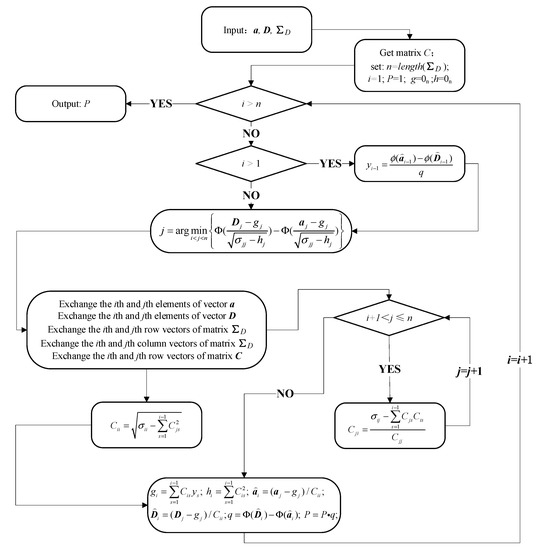
Figure 6.
Procedure of calculating the CDF value of the multivariate normal distribution by the univariate conditioning approximation method.
Step 3. Repeat the above steps at the next IM until the calculation is completed.
5. Numerical Analysis
5.1. The Modeling Details of the Bridge
A steel truss bridge with a span of 100 m + 400 m + 100 m was used as an example to illustrate the proposed component and the related system fragility analysis methods. The upper structural truss members of this bridge were made of Q345 and Q420 steel. The arch ribs of the main truss plates were box-shaped. The bracing and the web rods were box-shaped and I-shaped. The tie rods were box-shaped and H-shaped. The suspenders were composed of parallel steel wire with a standard strength of 1680 MPa. The bridge deck adopted a steel–concrete composite structure. The elevation layout of the bridge and the corresponding support restraint system of the bearings are shown in Figure 7 (details of the support restraint system are shown in the following paragraphs), and the heights of piers 1–4 were 19.5 m, 10.3 m, 10.3 m, and 20.5 m, respectively.
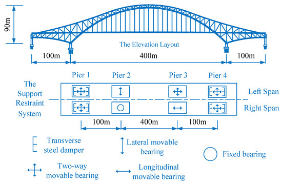
Figure 7.
The elevation layout and the support restraint system of the bridge.
The finite element (FE) model of the studied bridge was established by OPENSEES [48]. The deck beams and the deck slabs were simulated by elastic elements. The suspension rods and the tie rods were simulated by truss elements. The truss members, piers, and caps were simulated by elastic–plastic fiber section elements, and each truss member was modeled with a single element with five integration points. The supports and the dampers were simulated by zero-length elements, and the friction coefficient of the supports was set as 0.03. The effects of the group piles were simulated by the six-spring dampers model. According to Chinese guideline JTG-B01-2014, the design highway lane loads (Figure 8) were applied to all traffic lanes during the nonlinear time history analysis.
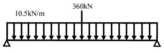
Figure 8.
Design highway lane loads.
It is important to note that when simulating the pier–beam connections, three constitutive models were used to present the mechanical characteristics of the bearing, the steel damper, and the displacement limiter, as shown in Figure 9. LS1–LS4 in the constitutive model of the displacement limiter represent the displacements corresponding to slight, moderate, severe, and absolute damage. The Fy in the constitutive model of the displacement limiter represents the designed maximum transverse force, as presented in Table 2. In the transverse direction, the LS3 of the fixed bearing was set as a very small value (because the bearing is unmovable in the fixed direction), and LS1–LS4 of the remaining bearings are displayed in Section 5.3.1. Aside from that, the vertical direction of the pier–beam connections was restricted, and the rotational stiffnesses of the zero-length elements were not considered.
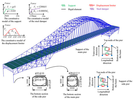
Figure 9.
The established bridge model and the used constitutive model.
Table 2.
The Fy in the constitutive model of the displacement limiter.
5.2. Determination of the Random Variables
5.2.1. The Seismic Uncertainties
Earthquakes exhibit strong randomness. Even at the same location, the recorded time history curves can be different. In time history analysis, structure ground motion samples should be selected to satisfy the site condition, fortification intensity, magnitude, epicentral distance, and so on. The Applied Technology Council (ATC) conducted a project entitled “Quantification of Building System Performance and Response Parameters” in 2009, in which they established the suggested ground motions for evaluating the structure responses [49]. The 20 far-field ground motions used in this paper were selected from the above ATC-63 database. The main purpose of this paper was to introduce the proposed fragility analysis methods, so only the transverse components of the ground motions were considered. In addition, inputting one component of the ground motions is common in bridge engineering. The transverse direction of bridges is vulnerable during earthquakes, so studying the influences caused by the transverse components of the ground motions is necessary. The selected ground motions are listed in Table 3. The peak ground acceleration (PGA) of each ground motion was adjusted from 0.2 g to 2 g (setting the interval as 0.2 g) by the IDA method.
Table 3.
The ground motion inputs.
5.2.2. The Structural Uncertainties
Uncertainties of the material properties and load effects will affect the bridge responses under earthquake conditions; therefore, these uncertainties must be considered (Table 4). Generally, the concrete compressive strength, the coefficient of the rebar strain hardening ratio, and the yield strength of the rebar are assumed to follow the normal or log-normal distribution [50,51,52,53]. In this research, the means of the concrete compressive strengths and the rebar yield strength were selected from related Chinese designed codes, and the coefficients of variation (CoVs) were picked from [35,50,51]. The uncertainty parameters of the rebar strain hardening ratio were adopted from [52,53]. It is worth noting that when the dead load (Phase I dead load + Phase II dead load) is considered as an uncertainty parameter, researchers generally assume it follows uniform distribution [52,54]. However, in Table 4, the Phase I dead load is ignored, and the Phase II dead load follows a normal distribution. The reason for this is that for the case study bridge, all truss members and bridge deck plates were well fabricated in factories, which meant the deviation of the actual and the design Phase I dead load was not significant. Therefore, the uncertainty of the Phase I dead load was not considered. While the Phase II dead load represents the dead load of prefabricated components, assuming it follows the normal distribution is also reasonable, and the relevant mean and COV were chosen from [50].
Table 4.
Random variables incorporated in the analytical bridge models.
5.2.3. The Uncertainties of the Seismic Capacity
The seismic capacity of the structural components is affected by a lot of factors. For example, the attitude of the workers and the concrete quality can affect the physical properties of the constructed bridge, and these factors influence the seismic capacity of the bridge components. Therefore, the seismic capacities were considered random variables as well. In bridge engineering, the seismic capacities of bridges are generally assumed to follow the log-normal distribution [38]. The used coefficient of variation (COV) of the slight damage (LS1) and the moderate damage (LS2) was 0.25, and the COV of the severe damage (LS3) and the absolute damage (LS4) was 0.5. The relationship between the COV and βc is shown in Equation (24):
According to Equation (24), the used βc for each LS was 0.246 (LS1), 0.246 (LS2), 0.472 (LS3), and 0.472 (LS4).
5.3. Determination of the Damage Index
5.3.1. The Damage Index of the Support
In this study, the maximum displacement was selected to represent the damage index (DI) of the movable bearing (support). Figure 10 displays the installed movable supports. The shadowed area represents the cushion stone, X and Y represent the longitudinal and transverse directions of the bridge, respectively, Y1 and Y2 represent the transverse length of the top plate and the base plate of the support, respectively, Y3 represents the transverse length of the cushion stone, X1 and X2 represent the longitudinal length of the top plate and the base plate of the support, respectively, and X3 represents the longitudinal length of the cushion stone. When the displacement of the bearing exceeds the design value but is within the support base plate, the bearing will be damaged slightly (LS1). When the edge of the support’s top plate exceeds the edge of the support’s base plate but does not exceed half of the distance from the edge of the support’s base plate to the edge of the cushion stone, the support will be damaged moderately (LS2). When the edge of the support’s top plate exceeds half of the distance from the edge of the support’s base plate to the edge of the cushion stone but is within the cushion stone, the support will be damaged severely (LS3). Once the edge of the support’s top plate exceeds the edge of the cushion stone, the support will be damaged absolutely (LS4). The support damage in the fixed direction was not considered. Table 5 and Table 6 display the DIs of the movable bearing in the transverse direction.
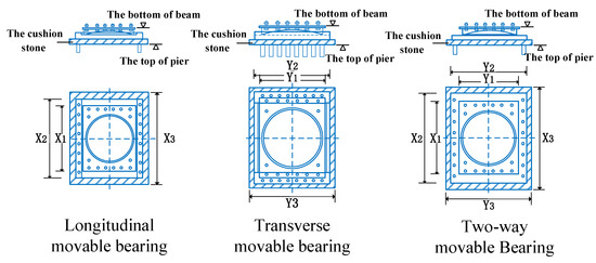
Figure 10.
Appearance of the movable bearings.
Table 5.
Illustration of the damage indexes of the bearing in the transverse direction.
Table 6.
The displacement damage indexes of the movable bearings in the transverse direction.
5.3.2. The Damage Index of the Pier
In this paper, the curvature was selected as the DI of the pier [12], and corresponding criteria to define the damage indexes are displayed in Table 7. The specific steps to determine the DI were as follows. First, obtain the maximum axial force of each pier by inputting the selected seismic waves (i.e., the seismic waves in Table 3 amplified by the IDA method) into the established FE model. Then, apply the maximum axial force and perform bending moment curvature analysis to each pier. Finally, determine the DI by matching the numerical results and the limit states in Table 7. The transverse curvature damage indexes of the studied bridge piers are listed in Table 8.
Table 7.
Criteria to define the curvature damage indexes of the piers.
Table 8.
The transverse curvature damage indexes of the studied bridge piers.
5.3.3. The Damage Index of the Steel Truss Member
Based on the structural characteristics of steel truss bridges, it can be known that damage caused by the transverse earthquake are mainly concentrated in the bridge supports and bridge piers. Therefore, only the slight (LS1) and moderate (LS2) damage states were set for the steel truss members. In accordance with [12], the yield strain and 10% of the ultimate elongation rate were set as LS1 and LS2 for the steel truss members individually.
6. Results and Discussion
6.1. Damage of the Steel Truss Members
Table 9 shows the damage states of the steel truss members after inputting a transverse seismic wave (the used wave was extended to 10 seismic waves with PGA ranges from 0.2 g to 2.0 g by the IDA method). It can be observed that no matter how strong the earthquake was, only a few truss members were damaged. Even when the PGA reached 2.0 g, only 1 truss member was damaged moderately. This means that the superstructure of the studied bridge was relatively strong under transverse seismic waves. Therefore, only the fragility of the piers and the supports were studied for the following section.
Table 9.
The damage states of the steel truss members under a transverse seismic wave.
6.2. Component Fragility
Figure 11 displays the proposed and original PSDM of the No. 1 left bearing. Figure 12 shows the related fragility curves. P and OG stand for the fragility curves generated by the proposed and the original PSDM, respectively. As can be seen, compared with the original PSDM, the proposed PSDM sensitively reflected the changing trend of the component demand with the fluctuation of the seismic intensity measure. In addition, for slight and moderate damage, when the PGA was between 0.5 g and 1.0 g, the fragility curves generated by the proposed PSDM (logarithmic piecewise function-based) was slightly lower than that of the original PSDM (logarithmic linear function-based). For severe and absolute damage, by increasing the PGA, the fragility curves generated by the proposed PSDM was first slightly lower than that of the original PSDM and then became slightly higher than it. In general, the fragility curves generated by the proposed and original PSDM were close to each other, and the proposed PSDM could solve the problem of mismatches in statistical significances between the PSDM and the JPSDM.
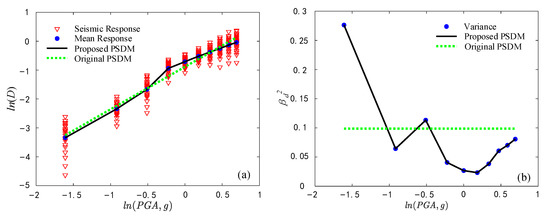
Figure 11.
(a) Logarithmic mean and (b) logarithmic variance of the PSDM of the No. 1 left bearing.
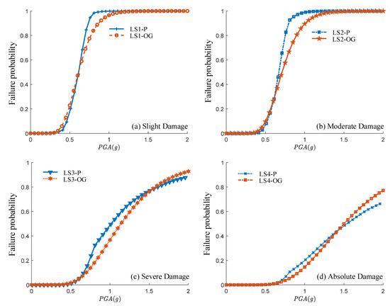
Figure 12.
Transverse component fragility curves of the No. 1 left bearing obtained by the proposed method and the original method.
Figure 13 shows the transverse fragility curves of the bridge piers obtained by the proposed method. It can be observed that (1) the side piers were more likely to be damaged than the main piers, (2) the failure probabilities of the severe damage and absolute damage were low, (3) for the side piers, because pier 4 was slightly higher than pier 1, the failure probability of pier 4 was slightly higher than that of pier 1, and (4) for the main piers, the constrains of the left span’s supports were weaker than those of the right span’s supports, so the failure probability of the right span’s piers were slightly higher than those of the left span’s piers.
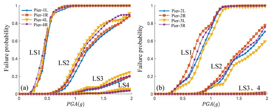
Figure 13.
The transverse fragility curves of (a) the side piers and (b) the main piers.
Figure 14 shows the transverse fragility curves of the bridge bearings obtained by the proposed method. By comparing Figure 13a and Figure 14a, it can be seen that except for the slight damage, the failure probabilities of the side piers were lower than those of the corresponding bearings, which means the bearings on the side piers were more likely to have moderate or higher levels of damage than the side piers themselves. Aside from that, in Figure 14a, the fragility curves of LS1 were near those of LS2. The reason for this was that LS1 and LS2 of the side bearings were close to each other (Table 6).
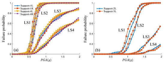
Figure 14.
The transverse fragility curves of (a) the side bearings and (b) the main bearings.
Since the damage of the fixed direction of the bearing was not considered, only the fragility curves of the left span’s main bearings were calculated, as shown in Figure 14b. By comparing Figure 14a,b, it was concluded that the main bearings had lower failure probabilities than those of the side bearings. The reason for this was that the restricted forces provided by the displacement limiters of the main bearings were much larger than those of the side bearings, as can be seen in Table 2. Therefore, in the same seismic event, the main bearing should have a smaller displacement (smaller failure probability). Aside from that, even when the main bearing and the side bearing reach the same displacements, the main bearings will have less of a chance to fail because the LSs of the two types of bearings are different, as displayed in Table 6. In addition, the failure probabilities of the main bearings were smaller than those of the main piers, which means by increasing the intensity measure, the main bearings were less likely to be damaged than the main piers.
6.3. The System Fragility
Figure 15 displays the transverse system fragility curves generated by the proposed method, where “LB-P” and “UB-P” are the lower and upper bounds of the system failure, respectively. They were calculated by combining the first-order reliability method with the components’ fragility curves generated by the logarithmic piecewise function-based PSDM. The “SYS-P” represents the system fragility curves. Figure 16 shows the transverse system fragility curves generated by traditional methods. Similarly, “LB-OG”, “UB-OG”, and “SYS-OG” represent the related lower, upper, and system fragility curves, respectively.
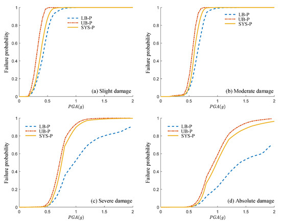
Figure 15.
The transverse system fragility curves generated by the proposed method.
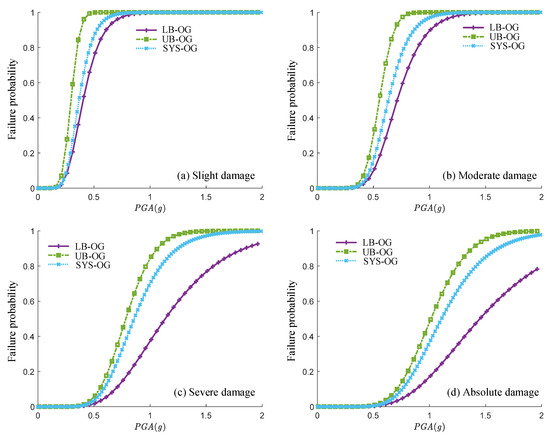
Figure 16.
The transverse system fragility curves generated by the traditional method.
As can be seen, no matter what the state of the damage was, “LB-P” and “LB-OG” (or “UB-P” and “UB-OG”) were close to each other. This happened because the component fragility curves generated by the proposed and the original methods were close to each other. Therefore, when calculating the failure bounds with Equation (10), the results should also be similar.
For severe and absolute damage, the proposed and traditional system fragility curves were close to the relevant failure upper bounds (i.e., SYS-OG was close to UB-OG, and SYS-P was close to UB-P). The reason for this was that the severe and absolute damage of the studied case were mainly determined by the damage to the supports. By checking the PSDM of those supports, it could be found that the standard deviation of each support (i.e., the standard deviation of the demand) was much smaller than the standard deviation of the relevant damage thresholds (i.e., the standard deviation of the capacity, which was 0.472 here). Therefore, when calculating the system failure probability, the diagonal elements of the generated covariance matrix of the multivariate joint normal distribution would be much larger than the other non-diagonal elements (i.e., the diagonal elements of matrix were larger than other non-diagonal elements). This means that this covariance matrix exhibited similar characteristics as the components were independent of each other, so the system failure probabilities were close to the corresponding failure upper bounds.
7. Conclusions
In this paper, the traditionally used logarithmic linear function-based probabilistic seismic demand model (PSDM) was replaced by the logarithmic piecewise function-based PSDM. This replacement made the sources and statistical significance of the parameters used in the PSDM and the JPSDM comparable and improved the fitting accuracy. Additionally, to improve the efficiency when calculating the system failure probabilities, the MCS method was replaced by the UCA method. The transverse seismic responses of a steel truss bridge were used to illustrate the feasibility of the proposed component and system fragility analysis methods. The results showed the following:
- The proposed methods unified the data sources and statistical significances of the parameters used in the PSDM and the JPSDM.
- The logarithmic piecewise function-based PSDM sensitively reflected the changing trend of the component demand with the fluctuation of the seismic intensity measure.
- Under transverse seismic waves, major damage happened to the side bearings of the bridge. Meanwhile, slight damage may have occurred on each pier. As the seismic intensity measure increased, the side bearings were more likely to be damaged.
- For the severe damage and the absolute damage of the studied bridge, the system fragility curves were close to the upper failure bounds.
- Compared with the Monte Carlo sampling method, the accuracy of the univariate conditioning approximation method could be guaranteed with less calculation time.
Author Contributions
Y.Z. and H.H. conceived the idea; Y.Z. and L.B. prepared the draft; H.C. and H.H. reviewed and edited the draft; M.T. and H.H. supervised the project; Y.Z. and D.S. collated the data. All authors have read and agreed to the published version of the manuscript.
Funding
This study was funded by the Science and Technology Planning Project of Guangzhou Municipal Construction Group Co., Ltd. ([2020]-KJ009), the Science and Technology Planning Project of Guangzhou (No.202102020684), and the Guangzhou Baiyun District Innovation and Entrepreneurship Leading Team Project (2021-0305). The financial support is gratefully acknowledged.
Institutional Review Board Statement
Not applicable.
Informed Consent Statement
Not applicable.
Data Availability Statement
The data used to support the findings of this study are available from the corresponding author upon request.
Conflicts of Interest
The authors declare no conflict of interest.
References
- Cornell, C.A.; Krawinkler, H. Progress and challenges in seismic performance assessment. PEER Cent. News 2000, 3, 1–3. [Google Scholar]
- Moehle, J.; Deierlein, G. A Framework Methodology for Performance-based Earthquake Engineering. In Proceedings of the 13th World Conference on Earthquake Engineering, Vancouver, BC, Canada, 1–6 August 2004; pp. 3812–3814. [Google Scholar]
- Wei, W.; Yuan, Y.; Igarashi, A.; Hongping, Z.; Ping, T. Experimental investigation and seismic fragility analysis of isolated highway bridges considering the coupled effects of pier height and elastomeric bearings. Eng. Struct. 2021, 233, 111926. [Google Scholar] [CrossRef]
- Hoang, P.; Phan, H.; Nguyen, D.; Paolacci, F. Kriging Metamodel-Based Seismic Fragility Analysis of Single-Bent Reinforced Concrete Highway Bridges. Buildings 2021, 11, 235–238. [Google Scholar] [CrossRef]
- Wei, B.; Hu, Z.; He, X.; Jiang, L. Evaluation of optimal ground motion intensity measures and seismic fragility analysis of a multi-pylon cable-stayed bridge with super-high piers in Mountainous Areas. Soil Dyn. Earthq. Eng. 2020, 129, 105945. [Google Scholar] [CrossRef]
- Liang, Y.; Yan, J.; Cheng, Z.; Chen, P.; Ren, C. Time-Varying Seismic Fragility Analysis of Offshore Bridges with Continuous Rigid-Frame Girder under Main Aftershock Sequences. J. Bridge Eng. 2020, 25, 04020055. [Google Scholar] [CrossRef]
- Zakeri, B.; Padgett, J.; Amiri, G. Fragility Analysis of Skewed Single-Frame Concrete Box-Girder Bridges. J. Perform. Constr. Facilities. 2014, 28, 571–582. [Google Scholar] [CrossRef]
- Banerjee, S. Statistical, Empirical and Mechanistic Fragility Analysis of Concrete Bridges; University of California: Irvine, CA, USA, 2007. [Google Scholar]
- Billah, M.A.; Alam, M.S. Seismic Fragility Assessment of Highway Bridges: A State-of-the-art Review. Struct. Infrastruct. Eng. 2015, 11, 804–832. [Google Scholar] [CrossRef]
- Cornell, C.; Jalayer, F.; Hamburger, R.; Foutch, D. Probabilistic Basis for 2000 SAC Federal Emergency Management Agency Steel Moment Frame Guidelines. J. Struct. Eng. 2002, 128, 526–533. [Google Scholar] [CrossRef] [Green Version]
- Pan, Y.; Agrawal, A.; Ghosn, M.; Alampalli, S. Seismic Fragility of Multispan Simply Supported Steel Highway Bridges in New York State. II: Fragility Analysis, Fragility Curves, and Fragility Surfaces. J. Bridge Eng. 2010, 11, 462–472. [Google Scholar] [CrossRef]
- Jiao, C.Y. Performance Based Seismic Fragility Analysis of Long-span Cable-stayed Bridges; Tongji University: Shanghai, China, 2008. [Google Scholar]
- Wu, C.H. Dynamic Time History Analysis of a Seven Story Concrete Shear Wall Model Structure Based on Plastic Damage Model. Guangzhou Archit. 2020, 48, 20–26. [Google Scholar]
- Chen, G.X.; Lu, J.; Lai, H.T. Structural Design and Seismic Resistance Performance Analysis of a Super High-rise Building in Shenzhen. Guangzhou Archit. 2019, 47, 3–6. [Google Scholar]
- Zhao, Y.; Yan, Q.; Yang, Z.; Yu, X.; Jia, B. A Novel Artificial Bee Colony Algorithm for Structural Damage Detection. Adv. Civ. Eng. 2020, 2020, 1–21. [Google Scholar] [CrossRef] [Green Version]
- Liu, H.; Zhang, Y. Bridge condition rating data modeling using deep learning algorithm. Struct. Infrastruct. Eng. 2020, 16, 1447–1460. [Google Scholar] [CrossRef]
- Zhao, Y.; Zhong, X.; Foong, L. Efficient metaheuristic-retrofitted techniques for concrete slump simulation. Smart Struct. Syst. 2021, 27, 745–759. [Google Scholar]
- Kim, H.; Kim, C. Deep-Learning-Based Classification of Point Clouds for Bridge Inspection. Remote. Sens. 2020, 12, 3757–3763. [Google Scholar] [CrossRef]
- Zhao, Y.; Xiaolin, Z.; Foong, L.K. Predicting the splitting tensile strength of concrete using an equilibrium optimization model. Steel Compos. Struct. 2021, 39, 81–93. [Google Scholar]
- Liang, X. Image-based post-disaster inspection of reinforced concrete bridge systems using deep learning with Bayesian optimization. Comput. Aided Civ. Infrastruct. Eng. 2018, 34, 415–430. [Google Scholar] [CrossRef]
- Zhao, Y.; Moayedi, H.; Bahiraei, M.; Foong, L.K. Employing TLBO and SCE for optimal prediction of the compressive strength of concrete. Smart Struct. Syst. 2020, 26, 753–763. [Google Scholar]
- Sheikh, I.; Khandel, O.; Soliman, M.; Haase, J.S.; Jaiswal, P. Seismic fragility analysis using nonlinear autoregressive neural networks with exogenous input. Struct. Infrastruct. Eng. 2021, 1–15. [Google Scholar] [CrossRef]
- Wang, Z.; Pedroni, N.; Zentner, I.; Zio, E. Seismic fragility analysis with artificial neural networks: Application to nuclear power plant equipment. Eng. Struct. 2018, 162, 213–225. [Google Scholar] [CrossRef] [Green Version]
- Segura, R.; Padgett, J.; Paultre, P. Metamodel-Based Seismic Fragility Analysis of Concrete Gravity Dams. J. Struct. Eng. 2020, 146, 04020121. [Google Scholar] [CrossRef] [Green Version]
- Li, H.; Li, L.; Zhou, G.; Xu, L. Time-dependent Seismic Fragility Assessment for Aging Highway Bridges Subject to Non-uniform Chloride-induced Corrosion. J. Earthq. Eng. 2020, 1–31. [Google Scholar] [CrossRef]
- Zhong, J.; Jeon, J.; Yuan, W.; DesRoches, R. Impact of Spatial Variability Parameters on Seismic Fragilities of a Cable-Stayed Bridge Subjected to Differential Support Motions. J. Bridge Eng. 2017, 22, 04017013. [Google Scholar] [CrossRef]
- Wu, W.P.; Li, L.; Shao, X. Seismic Assessment of Medium-Span Concrete Cable-Stayed Bridges Using the Component and System Fragility Functions. J. Bridge Eng. 2016, 21, 04016027. [Google Scholar] [CrossRef]
- Yılmaz, M.; Çağlayan, B. Seismic assessment of a multi-span steel railway bridge in Turkey based on nonlinear time history. Nat. Hazards Earth Syst. Sci. 2018, 18, 231–240. [Google Scholar] [CrossRef] [Green Version]
- Herath, N.; Mendis, P.; Zhang, L. A probabilistic study of ground motion simulation for Bangkok soil. Bull. Earthq. Eng. 2016, 15, 1925–1943. [Google Scholar] [CrossRef]
- Chen, X. System Fragility Assessment of Tall-Pier Bridges Subjected to Near-Fault Ground Motions. J. Bridge Eng. 2020, 25, 04019143. [Google Scholar] [CrossRef]
- Wu, W.P.; Li, L.F.; Wang, L.H. Evaluation of seismic vulnerability of high-pier long-span bridge using incremental dynamic analysis. J. Earthq. Eng. Eng. Vib. 2012, 32, 117–123. [Google Scholar]
- Pan, Y.; Agrawal, A.; Ghosn, M. Seismic Fragility of Continuous Steel Highway Bridges in New York State. J. Bridge Eng. 2007, 12, 689–699. [Google Scholar] [CrossRef]
- Cao, Y.; Liang, Y.; Huai, C.; Yang, J.; Mao, R. Seismic Fragility Analysis of Multispan Continuous Girder Bridges with Varying Pier Heights considering Their Bond-Slip Behavior. Adv. Civ. Eng. 2020, 2020, 8869921. [Google Scholar] [CrossRef]
- Qin, H.; Stewart, M. System fragility analysis of roof cladding and trusses for Australian contemporary housing subjected to wind uplift. Struct. Saf. 2019, 79, 80–93. [Google Scholar] [CrossRef]
- Mangalathu, S.; Heo, G.; Jeon, J. Artificial neural network based multi-dimensional fragility development of skewed concrete bridge classes. Eng. Struct. 2018, 162, 166–176. [Google Scholar] [CrossRef]
- Zhou, T.; Li, A.; Wu, Y. Copula-based seismic fragility assessment of base-isolated structures under near-fault forward-directivity ground motions. Bull. Earthq. Eng. 2018, 16, 5671–5696. [Google Scholar] [CrossRef]
- Xu, H.; Gardoni, P. Multi-level, multi-variate, non-stationary, random field modeling and fragility analysis of engineering systems. Struct. Saf. 2020, 87, 101999. [Google Scholar] [CrossRef]
- Nielson, B.G. Analytical Fragility Curves for Highway Bridges in Moderate Seismic Zones; Georgia Institute of Technology: Atlanta, GA, USA, 2005. [Google Scholar]
- Wang, Q.; Wu, Z.; Liu, S. Multivariate Probabilistic Seismic Demand Model for the Bridge Multidimensional Fragility Analysis. KSCE J. Civ. Eng. 2018, 22, 3443–3451. [Google Scholar] [CrossRef]
- Padgett, J.E. Seismic Vulnerability Assessment of Retrofitted Bridges Using Probabilistic Methods; Georgia Institute of Technology: Atlanta, GA, USA, 2007. [Google Scholar]
- Li, L.; Hu, S.; Wang, L. Seismic fragility assessment of a multi-span cable-stayed bridge with tall piers. Bull. Earthq. Eng. 2017, 15, 3727–3745. [Google Scholar] [CrossRef]
- Bakalis, K.; Vamvatsikos, D. Seismic Fragility Functions via Nonlinear Response History Analysis. J. Struct. Eng. 2018, 144, 04018181. [Google Scholar] [CrossRef]
- Zheng, K.F.; Chen, L.B.; Zhuang, W.L. Bridge Vulnerability Analysis Based on Probabilistic Seismic Demand Models. Gongcheng Lixue 2013, 30, 165–171, 187. [Google Scholar]
- Zhao, G.F.; He, S.; Ma, Y.H. Fragility Analysis of Offshore Isolated Bridge Based on Steel Pitting Corrosion Effect. China J. Highw. Transp. 2016, 29, 67–76. [Google Scholar]
- Yu, X.H.; Lv, D.G. Probabilistic Seismic Demand Analysis and Seismic Fragility Analysis Based on a Cloud-stripe Method. Gongcheng Lixue 2016, 33, 68–76. [Google Scholar]
- Trinh, G.; Genz, A. Bivariate Conditioning Approximations for Multivariate Normal Probabilities. Stat. Comput. 2014, 25, 989–996. [Google Scholar] [CrossRef]
- Gilat, A. MATLAB; Wiley: New York, NY, USA, 2016. [Google Scholar]
- McKenna, F.; Scott, M.; Fenves, G. Nonlinear Finite-Element Analysis Software Architecture Using Object Composition. J. Comput. Civ. Eng. 2010, 24, 95–107. [Google Scholar] [CrossRef]
- FEMA. Quantification of Building Seismic Performance Factors; FEMA: Washington, DC, USA, 2009.
- Dong, J.; Shan, D.S.; Zhang, E.H.; Ma, T. Near and Far-field Seismic Fragility Comparative Analysis of Irregular Bridge. J. Harbin Inst. Technol. 2016, 48, 159–165. [Google Scholar]
- Stefanidou, S.; Sextos, A.; Kotsoglou, A.; Lesgidis, N.; Kappos, A. Soil-structure interaction effects in analysis of seismic fragility of bridges using an intensity-based ground motion selection procedure. Eng. Struct. 2017, 151, 366–380. [Google Scholar] [CrossRef]
- Yan, L.F. Seismic Fragility Analysis of Steel Frame with Semi-Rigid Nodes; Southeast University: Nanjing, China, 2015. [Google Scholar]
- Li, H.; Li, L.; Wu, W.; Xu, L. Seismic fragility assessment framework for highway bridges based on an improved uniform design-response surface model methodology. Bull. Earthq. Eng. 2020, 18, 2329–2353. [Google Scholar] [CrossRef]
- Mangalathu, S.; Hwang, S.; Choi, E.; Jeon, J.S. Rapid seismic damage evaluation of bridge portfolios using machine learning techniques. Eng. Struct. 2019, 201, 109785. [Google Scholar] [CrossRef]
Publisher’s Note: MDPI stays neutral with regard to jurisdictional claims in published maps and institutional affiliations. |
© 2021 by the authors. Licensee MDPI, Basel, Switzerland. This article is an open access article distributed under the terms and conditions of the Creative Commons Attribution (CC BY) license (https://creativecommons.org/licenses/by/4.0/).