Application of Satellite-Based and Observed Precipitation Datasets for Hydrological Simulation in the Upper Mahi River Basin of Rajasthan, India

Abstract

Hydrological modeling is an important tool used for basin management and studying the impacts of extreme events in a river basin. In streamflow simulations, precipitation plays an essential role in hydrological models. Meteorological satellite precipitation measurement techniques provide highly accurate rainfall information with high spatial and temporal resolution. In this analysis, the tropical rainfall monitoring mission (TRMM) 3B42 V7 precipitation products were employed for simulating streamflow by using the soil water assessment tool (SWAT) model. With India Metrological Department and TRMM data, the SWAT model can be used to predict streamflow discharge and identify sensitive parameters for the Mahi basin. The SWAT model was calibrated for 2 years and then independently validated for 2 years by comparing observed and simulated streamflow. A strong correlation was observed between the calibration and validation results for the Paderdibadi station, with a Nash–Sutcliffe efficiency of >0.34 and coefficient of determination (R²) of >0.77. The SWAT model was used to adequately simulate the streamflow for the Upper Mahi basin with a satisfactory R² value. The analysis indicated that TRMM 3B42 V7 is useful in SWAT applications for predicting streamflow and performance and for sensitivity analysis. In addition, satellite data may require correction before its utilization in hydrological modeling. This study is helpful for stakeholders in monitoring and managing agricultural, climatic, and environmental changes.

1. Introduction

Global precipitation information is crucial for forecasting weather, climate, flood, drought, and understanding hurricanes and other weather phenomenon [1]. However, precipitation measurement is a challenge for meteorology because precipitation occurs with space and time variability [2]. Therefore, high-resolution precipitation data are important for hydrological applications [3]. The basic understanding of the spatial and temporal changeability of hydrological variables are essential for human life on earth, and environmental problems are observed in the principal vital resource, that is, river water [4]. Quantification of hydrological cycle components is essential in the modeling process, and precipitation plays the main role in the hydrological process. The quantity of precipitation depth and volume is also critical for estimating hazards and function of civil structures (e.g., reservoirs, dams, and bridges) and runoff models and resolving water-related problems (e.g., pollution, flooding, and drought) [5].

Rainfall is an extremely dynamic process to intensity over space and time, which makes it a critical issue. Three rainfall estimation methods are available: (1) rain gauge, (2) ground-based radar, and (3) satellite rainfall estimation [6]. Satellite rainfall estimation is used to derive precipitation data from radiance measured with a satellite by using visible- and infrared-based methods, active and passive microwave (MW) techniques, and combined infrared and MW approaches [7].

TRMM is a joint project between the United States Space Agency National Aeronautics and Space Administration (NASA) and Japan Aerospace Exploration Agency launched in November 1997. This project aims to accurately measure precipitation and associated latent heat over the tropical and subtropical regions because latent heat plays an important role in climate variations [8]. TRMM precipitation radar provides highly accurate high-resolution satellite-based rainfall data [9]. Some of the studies used the satellite data like precipitation, evapotranspiration to estimate the effect of these variables in flood prediction, streamflow analysis, water resources management [10,11,12,13,14,15,16]. TRMM 3B42 V7 algorithms provide three hourly temporal and 0.25° × 0.25° spatial resolution, extending from 50° south to 50° north latitude and 180° west to 180° east longitude globally and these products are based on the multi-satellite precipitation analysis [17].

The SWAT model may prove to be effective for describing monthly runoff from small watersheds [18]. Previous studies have frequently used the SWAT model for agricultural management, climate and land use/land cover (LULC) change management, and water resource management [19,20,21,22]. The SWAT model has been utilized for climate change impact assessments on Indian river basins by employing past, present, and future climate scenarios [23,24,25]. The model has also been used for several comparative studies related to the performance of national water services (NWS), NEXRAD stage III, TRMM 3B42 V6, rain gauge, NWS multi-sensor precipitation estimator, TRMM, multi-satellite precipitation analysis, TRMM 3B42 V6, and climate prediction center morphing method data for measuring the streamflow and sensitive parameters of various watershed systems [12,26,27]. The US National Water Model is well-developed to make a coupled model for interacting with land-atmosphere and used the satellite based data for the flood forecasting, extreme rainfall and streamflow analysis in the different watersheds [28,29,30,31,32]. This study utilized TRMM 3B42 V7 precipitation products for the Upper Mahi basin located above the Paderdibadi-30 rain gauge site. The overall goal of the present study was to evaluate the streamflow of Upper Mahi River Basin of Rajasthan, India. Considering the data limitation in this basin, the study to gain insights into the variation of water balance components of the basin. The main objective of the present study was: (i) to calibrate and validate the SWAT model for simulating streamflow in the basin, and (ii) to analyze the streamflow and water balance components of basin using the satellite based and gauge station precipitation datasets.

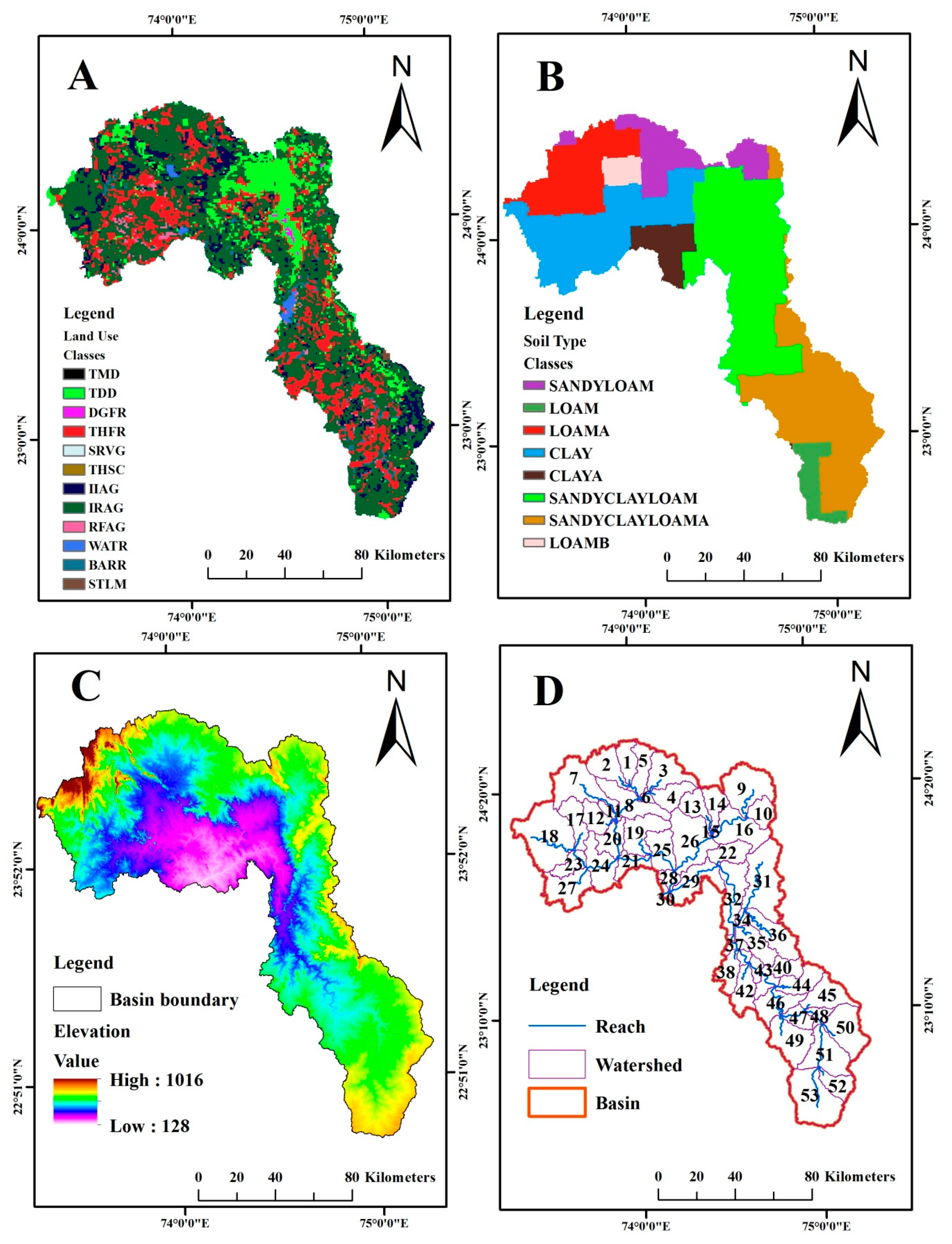
2. Description of Study Area

The Mahi basin extends over Rajasthan, Madhya Pradesh, and Gujarat covering 34,842 km², which is 1.1% area of India. It lies between 72°21′ to 75°19′ East longitude and 21°46′ to 24°30′ North latitude. Aravali hills bind this basin in the northwest direction, Malwa plateau on the eastern side, the Vindhyas on the southern side, and the Gulf of Khambhat on the western side. Mahi River originates in the Mahi Kanta hills (western part) of Madhya Pradesh in the Vindhyachal range [33].

The Mahi basin forms a “U” molded circle in Rajasthan before entering Gujarat and lastly discharges into the Gulf of Cambay. The main streams of the Mahi River are Som, Jakham, Moran, Anas, and Bhadar [33]. The Mahi River is divided into two parts: Upper and Lower Mahi basins. The present study was conducted on the Upper Mahi basin rain gauge station Paderdibadi (Figure 1), covering an area of 16,247 km² (46.63% of the total basin area) [34].

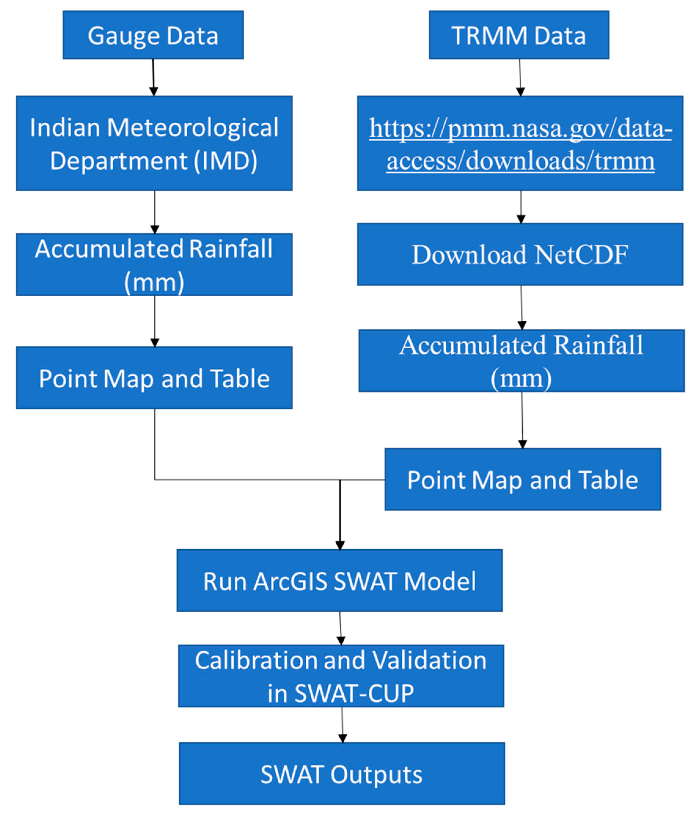
3. Data and Methodology

3.1. Discharge and Meteorological Data

In this analysis, stream discharge data of the Paderdibadi station site, obtained from the India WRIS Portal (8 http://www.india-wris.nrsc.gov.in/, accessed on 8 March 2019), were used (Figure 1). The gauge is located at latitude 23.75 and longitude 74.13 and has a contributing area of 16,247 Sq. Km.

India Meteorological Department (IMD) provided the rain gauge data. IMD monitors and maintains a record of all meteorological phenomena, including daily rainfall data of the whole nation. Rain gauge stations were considered for this study, as mentioned in Figure 1. The TRMM product 3B42 V7 data were used for the Upper Mahi basin. The TRMM data were downloaded from the NASA website (https://pmm.nasa.gov/data-access/downloads/trmm, accessed on 3 January 2019); latest LEVEL 3 data were available in the form of NetCDF, HDF, GEO-TIFF, and ASCII. The precipitation data of the 1998–2001 period were used as input in the SWAT model. The weather data were obtained from the IMD with daily temporal resolution.

3.2. Physical Data

In the present study, the National Remote Sensing Center land use data were used. Figure 2A shows the land use information of the Mahi basin. Some abbreviations were used for LULC (detailed information in

Table 1. Land Use/Land Cover and soil code with abbreviations.

Code	Land Use/Land Cover
TMD	Tropical, Dry Decidous Forest
TDD	Tropical Moist Forest
DGFR	Degraded Forest
THFR	Thom Forest/Shurb
SRVG	Sparse Vegetation
THSC	Thom Shurb/Desert
IIAG	Irrigated Intensive Agricultural
IRAG	Irrigated Agricultural Land
RFAG	Rainfed Agricultural
WATR	Water
BARR	Barren
STLM	Settlement
Code	Soil Type
SALO	SANDYLOAM
LOAM	LOAM
LOMA	LOAMA
CLAY	CLAY
CLYA	CLAYA
SCLO	SANDYCLAYLOAM
SCLA	SANDYCLAYLOAMA
LOMB	LOAMB

). The code of LULC and soil was used in the SWAT model. The soil data are mainly obtained from the Food and Agriculture Organization of the United Nations (FAO-US). Some abbreviations were used to denote soil type (

Table 2. Sensitive parameters with t-stat and p value.

Parameter_Name	Descriptions of Parameters	t-Stat	p-Value	Rank
V__SLSUBBSN.hru	Average slope length	11.88	0	1
V__SOL_BD(..).sol	Moist bulk density	−3.41	0	2
V__ESCO.hru	Soil evaporation compensation factor	3.95	0	3
V__CH_K2.rte	Effective hydraulic conductivity in the main channel alluvium	2.36	0.02	4
R__SOL_K(..).sol	Saturated hydraulic conductivity	−2.18	0.03	5
V__GW_DELAY.gw	Groundwater delay (days)	0.13	0.9	6
V__CH_N2.rte	Manning’s “n” value for the main channel	1.61	0.11	7
V__ALPHA_BNK.rte	Baseflow alpha factor for bank storage	−1.56	0.12	8
R__CN2.mgt	SCS runoff curve number	1.23	0.22	9
V__GWQMN.gw	Threshold depth of water in the shallow aquifer required for return flow to occur (mm)	−0.96	0.34	10
V__REVAPMN.gw	Threshold depth of water in the shallow aquifer for “revap” to occur (mm)	0.9	0.37	11
V__RCHRG_DP.gw	Deep aquifer percolation fraction	0.9	0.37	12
V__EPCO.hru	Plant uptake compensation factor	−0.84	0.41	13
R__SOL_AWC(..).sol	Available water capacity of the soil layer	0.51	0.61	14
V__ALPHA_BF.gw	Baseflow alpha factor (days)	0.33	0.74	15

), and Figure 2B presents the soil map of the basin. The SRTM DEM data were obtained from NASA’s website (http://www2.jpl.nasa.gov/srtm/, accessed on 12 February 2019). A digital elevation model (DEM) is the raster data comprising an array of cells or pixels containing elevation values. Figure 2C shows the DEM information of the river basin. Figure 2D presents the SWAT watershed delineation tool output of the basin, the subbasins, and the stream network generated using DEM data. Figure 3 presents the steps required to form a complete database by comparing the satellite estimates with the observed surface runoff and running the SWAT hydrological model using satellite and rain gauge data.

3.3. SWAT Model Description

The SWAT model [35] was established by the U.S. Department of Agriculture, Agricultural Research Service in the early 1990s. It is a physically based, semi-distributed and continuous time step hydrologic model [36,37]. The SWAT model can analyze variation in hydrological processes, vegetation development, erosion, and water quantity and quality in larger basins [38,39,40]. This model uses the characteristics of topography, land use, and soil and management systems to generate slope, basin boundary, sub-basins, and hydrological response units (HRUs). The model also calculates water balance of the hydrological cycle based on control climate inputs. Using daily inputs, the SWAT model simulates daily, monthly, and yearly water balance in river basins. Simulations consider the main basin channel and calculate the quantity of water, sediment yield, and pollutants [27]. The water balance of the basin is calculated using the following equation in the SWAT model:

$$\mathrm{S}{\mathrm{W}}_{\mathrm{t}}=\mathrm{S}{\mathrm{W}}_0+{\displaystyle \sum }_{i=1}^{\mathrm{t}}\left({\mathrm{R}}_{\mathrm{d}\mathrm{a}\mathrm{y}}-{\mathrm{Q}}_{\mathrm{s}\mathrm{u}\mathrm{r}\mathrm{f}}-{\mathrm{E}}_{\mathrm{a}}-{\mathrm{W}}_{\mathrm{s}\mathrm{e}\mathrm{e}\mathrm{p}}-{\mathrm{Q}}_{\mathrm{g}\mathrm{w}}\right)$$

(1)

where SW_t = soil water on day t, SW₀ = initial soil water, R_day = rainfall, Q_surf = surface runoff, E_a = actual evaporation, W_seep = water seepage, and Q_gw = groundwater recharge.

3.4. SWAT-CUP Model (SUFI-2 Algorithm)

Model calibration requires a change in model parameters. The sequential uncertainties fitting ver-2 (SUFI-2) algorithm was used to calibrate and validate the SWAT model. The SWAT-CUP model is used to calibrate and validate the SWAT model and provide the link between SWAT and SWAT-CUP [41]. The SUFI-2 optimization algorithm defined the model uncertainty between observed and simulated variable deviations. The SUFI-2 algorithm analyzes the sensitivity of the calibrated parameters for model performance. The model is calibrated by using the p-factor and r-factor. The p-factor is defined as a percentage by 95% prediction uncertainty (95PPU). The r-factor indicates the average thickness of 95PPU. The r-factor indicates the thickness of the 95PPU band, and the p-factor ranges between 0% and 100%. However, the r-factor ranges from 0 to infinity. For better replication, the p-factor should be close to 1, whereas the r-factor should be close to zero.

3.5. Statistics Used for Performance Evolution

SWAT model performance was estimated using the graphical representation of observed and simulated discharge values. The performance of simulated results can also be calculated using various statistical parameters such as R² and Nash–Sutcliffe efficiency (NSE) [41]. The R² was used to evaluate variation in observed and simulated values. R² values vary from −1 to 1, where 1 is the perfect positive trend and −1 is the perfect negative trend. NSE values range between −∞ and 1. The equations for calculating NSE and R² are as follows:

$$R^2=\frac{{\left[{\sum }_i(Q_{m,i}-\overline{Q_m})(Q_{s,i}-\overline{Q_s})\right]}^2}{{{\displaystyle \sum }}_i{(Q_{m,i}-\overline{Q_m})}^2{{\displaystyle \sum }}_i{(Q_{s,i}-\overline{Q_s})}^2}$$

(2)

$$NSE=1-\frac{{\sum }_i{(Q_m-Q_s)}^2{}_i}{{\sum }_i{(Q_{m,i}-\overline{Q_m})}^2}$$

(3)

where Q_m = measured discharge value, Q_s = simulated discharge, Q_m(bar) = average measured discharge, and Q_s (bar) = average discharge simulated.

4. Results and Discussion

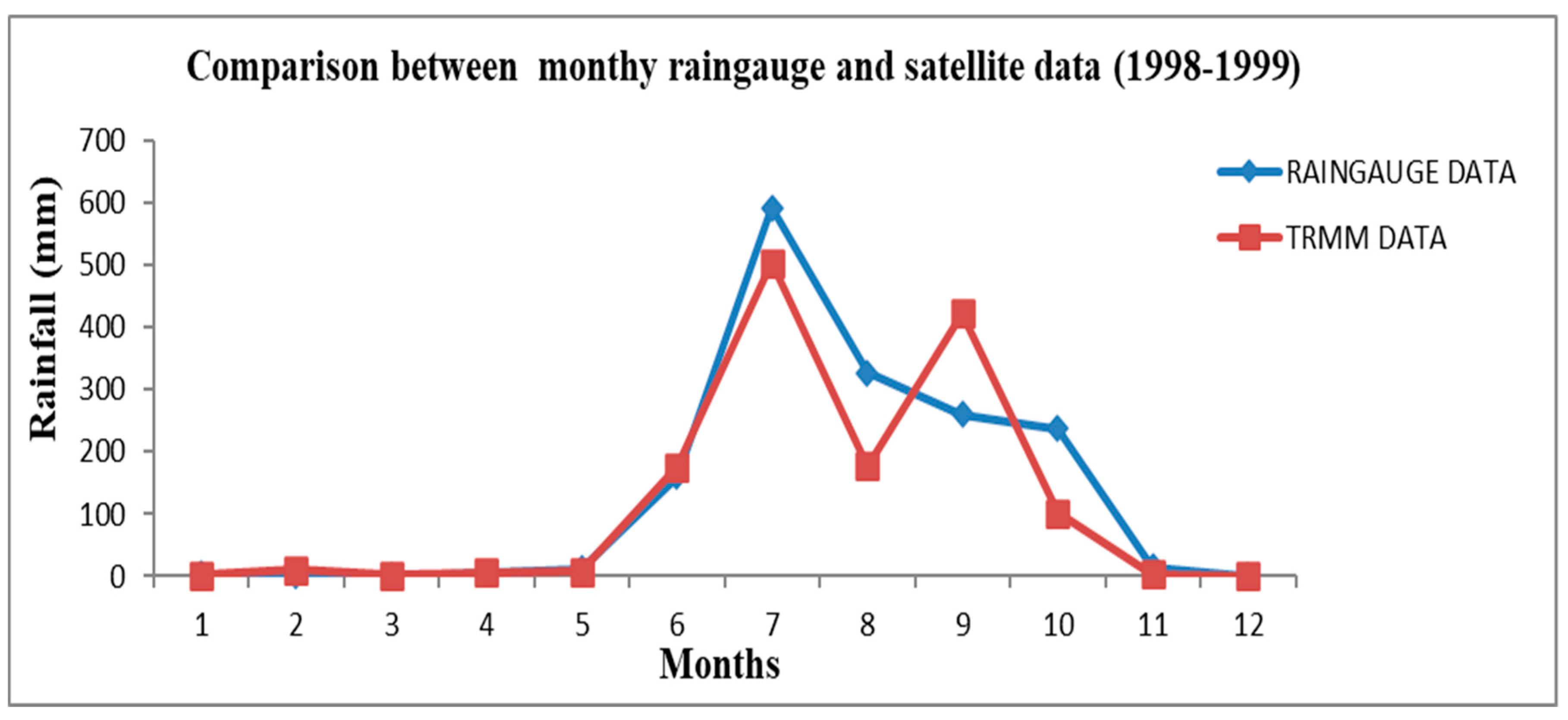
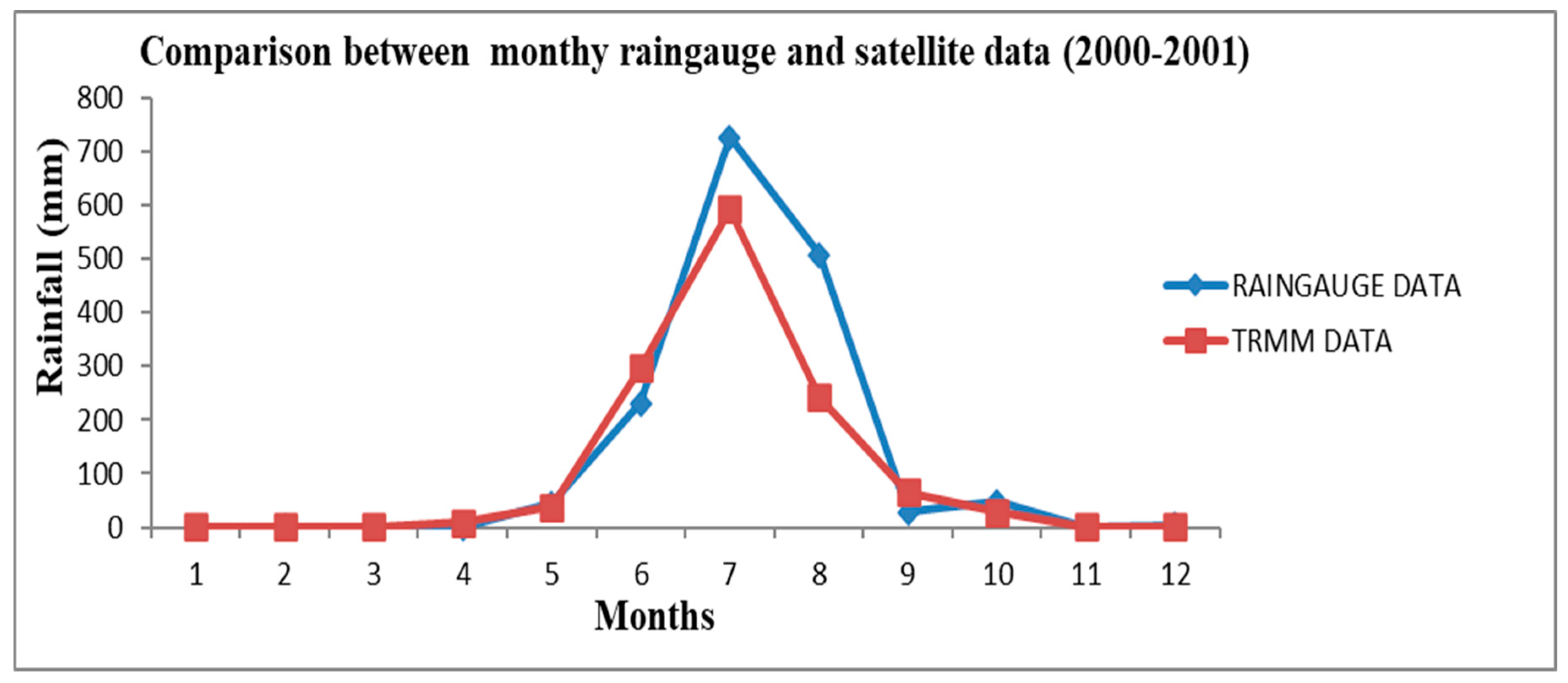
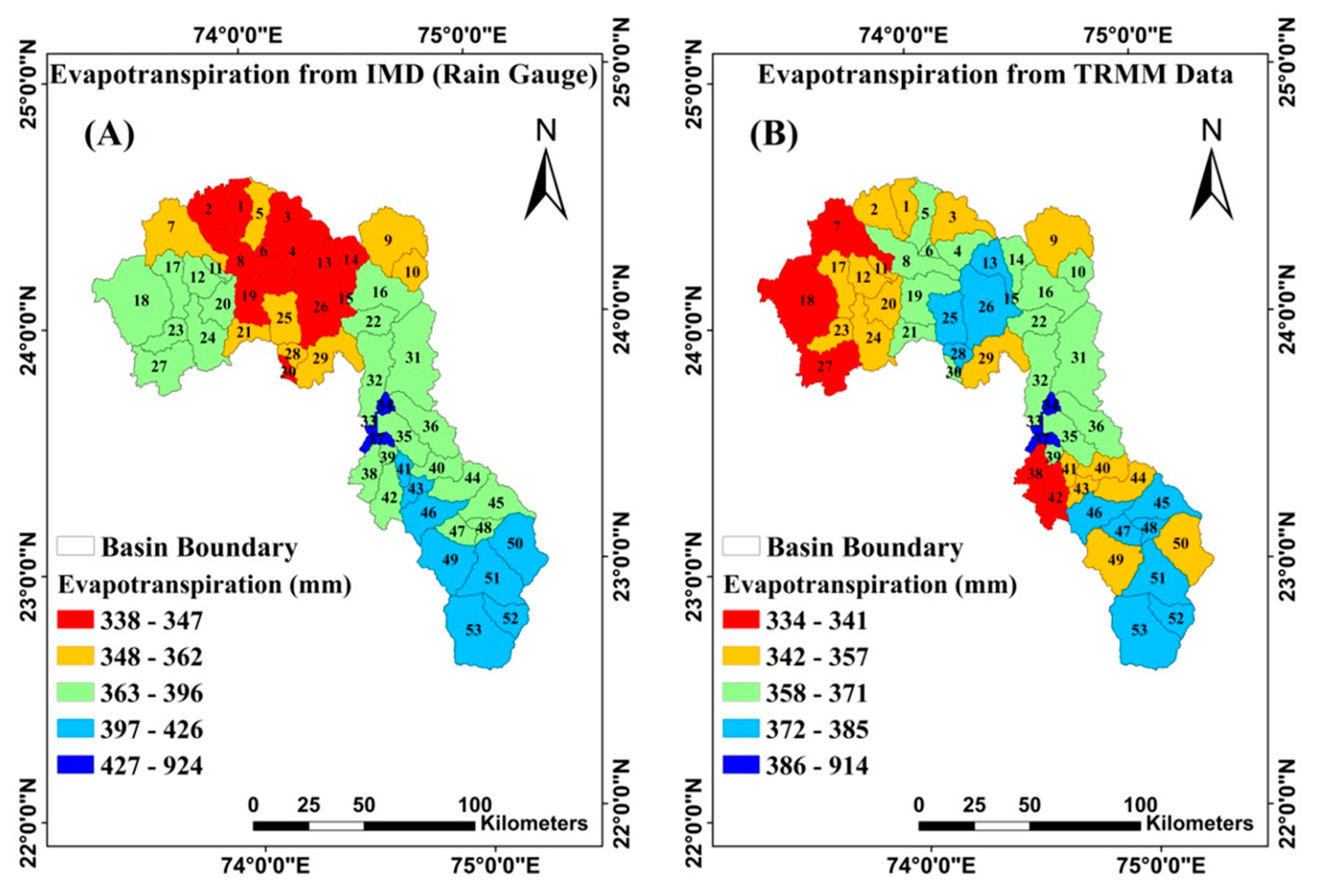
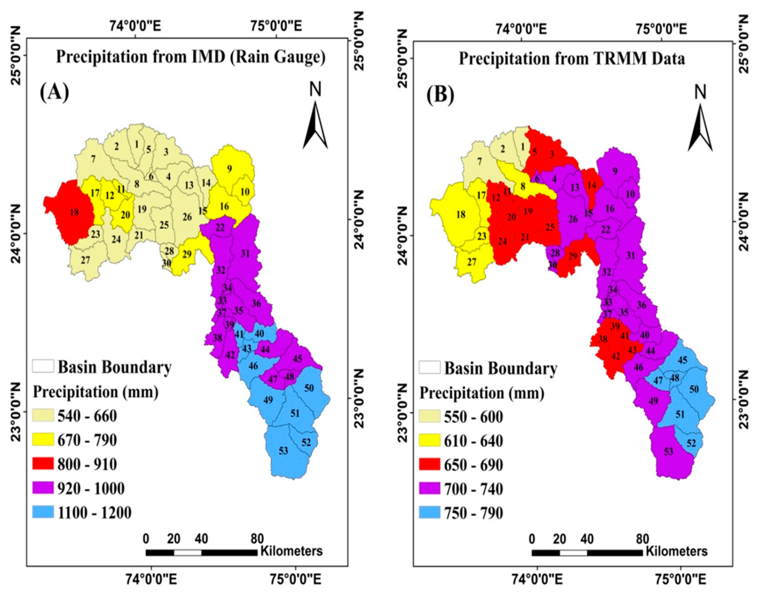
4.1. Comparison between Rain Gauge and TRMM Data

In Figure 4, line graphs plotted against monthly rain gauge and TRMM data for the calibration period (1998–1999) indicate that the TRMM and rain gauge data are similar. However, some bias was present in TRMM data due to instrumental and computation errors. Figure 4 shows that the highest rainfall was observed in July. The highest rainfall was 593.40 and 504.71 mm during the calibration period according to the rain gauge and TRMM data, respectively. In Figure 5, line graphs were plotted against both the rain gauge and TRMM data for the validation period (2000–2001). The highest rainfall was again observed in July (rain gauge data: 724.85 mm; TRMM data: 591.49 mm). These results indicate that this method is highly effective during the monsoon season and valuable for flood control.

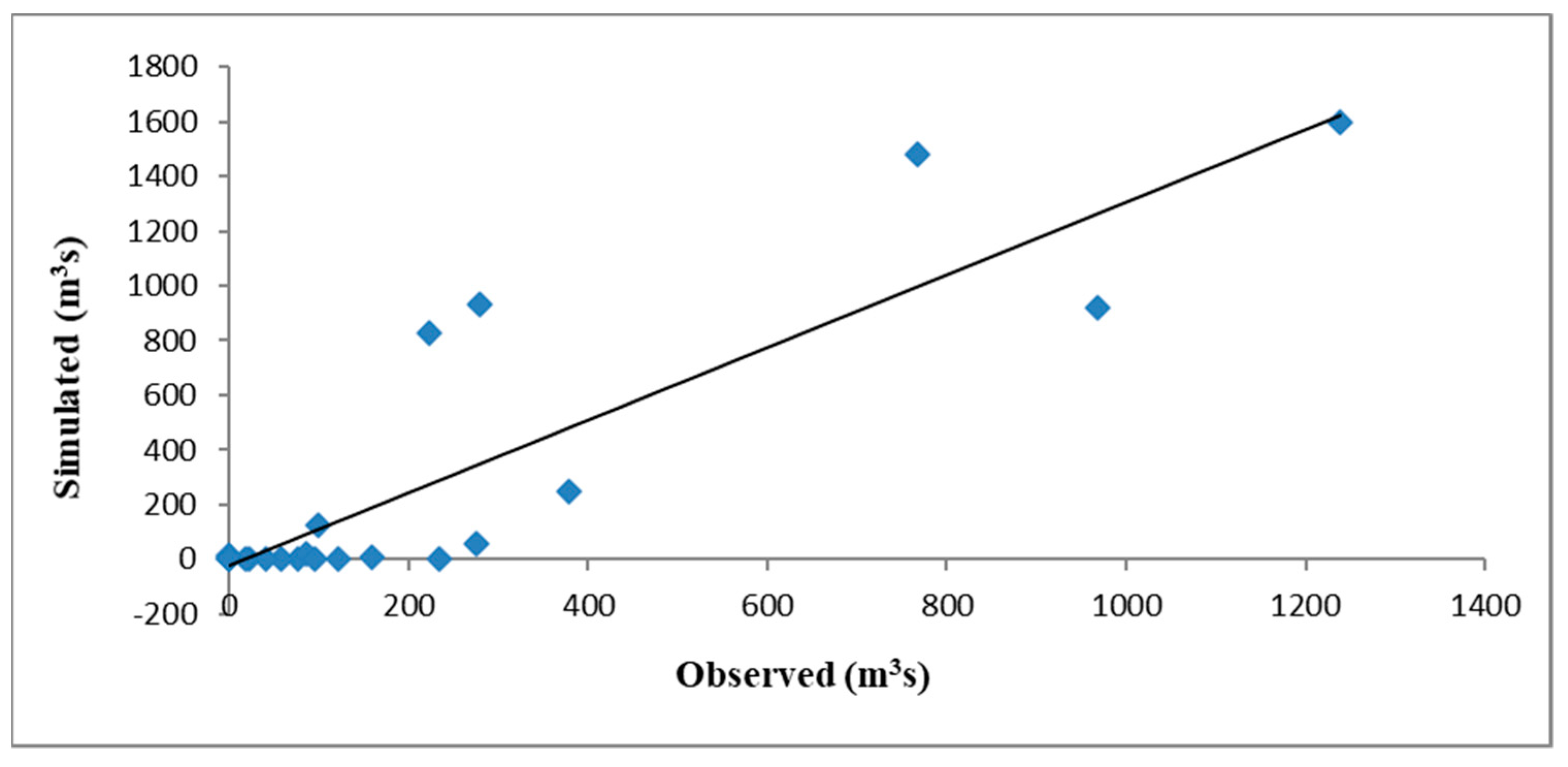
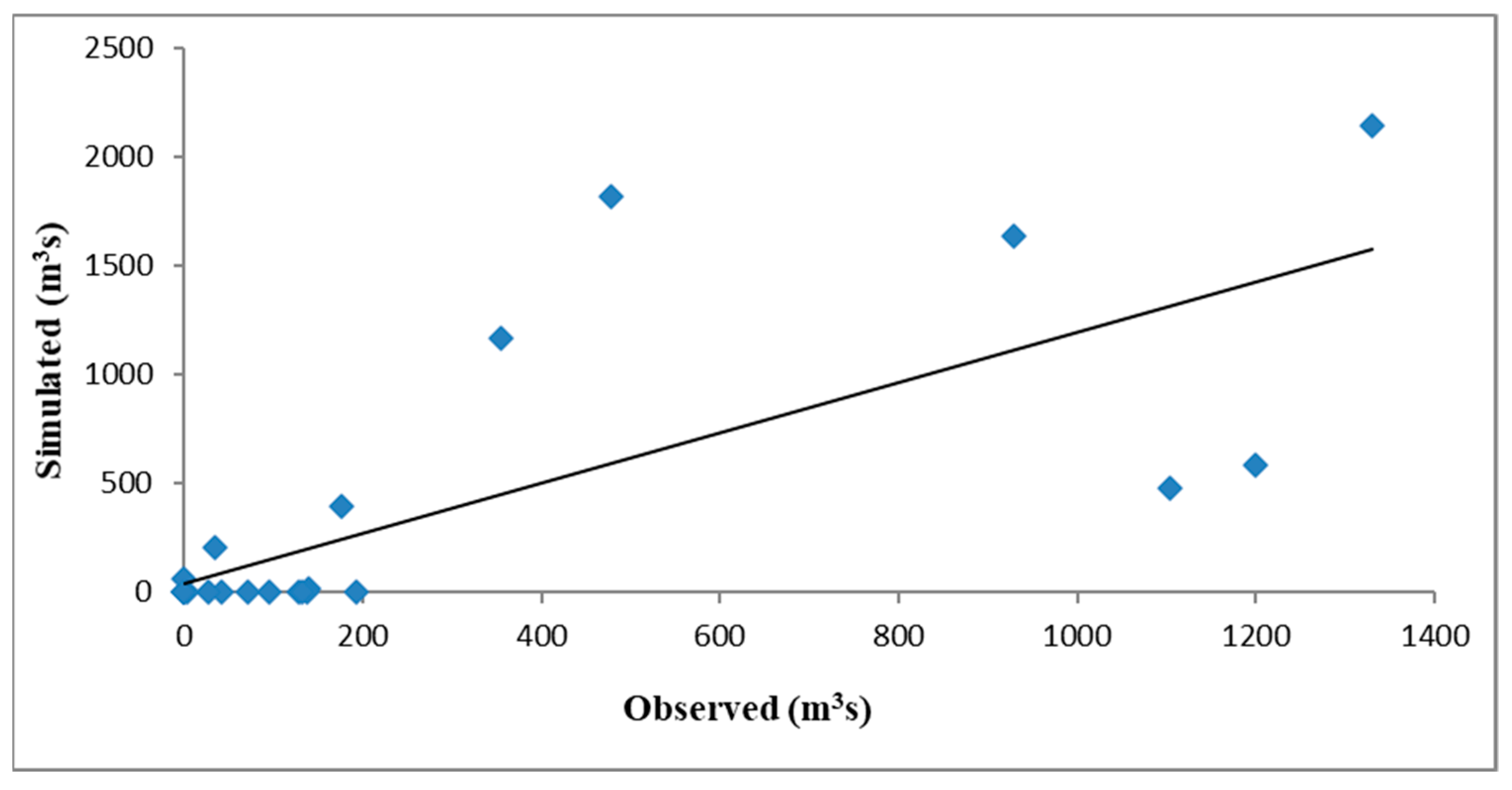
4.2. Calibration, Validation and Sensitivity Analysis

The SWAT model was calibrated and validated using the SWAT-CUP model, and the sensitive parameters were obtained using the observed discharge data from the Paderdibadi gauge station. The SWAT-CUP model provides sensitivity parameters by executing a multiple regression study. The t-test and p values are used to estimate the significance of the parameters, and p ≤ 0.05 shows the sensitivity and ranking of the parameters. In this analysis, fifteen parameters were used for the sensitivity analysis, and SLSUBBSN.hru was found to be the most sensitive parameter, followed by SOL_BD(..).sol, CH_K2.rte, SOL_K(..).sol, and ESCO.hru. Table 2 presents the rank and sensitivity of each parameter used for calibration and validation.

Model performance was computed using R² values. Figure 6 presents the plot of calibration period scatter against observed and simulated streamflow values for the watershed outlet Paderdibadi station. An R² statistic value of 0.77 was obtained during the calibration period (Figure 6). Figure 7 presents the validation period scatter plot against observed and simulated streamflow values. An R² value of 0.55 was obtained during the validation period (Figure 7). The R² computed result revealed that the simulated data for Paderdibadi showed a strong correlation with observed data. The R² value and other parameters were in optimal ranges (

Table 3. Calibration and validation performance of the observation site (Paderdibadi).

	p-Factor	r-Factor	R2	NSE
Calibration	0.08	0.08	0.77	0.34
Validation	0.17	0.07	0.55	−0.15

). This basin has several tributaries and dams. Therefore, the Paderdibadi station shows deviation from the optimum values and strong correlation when statistical and sensitive parameters are applied. This study has the limitations of data nonavailability for dam operations and presents the deviation for the Paderdibadi station in observed values. The variation in the values observed at the station might be revised by including the dam observational data in SWAT applications. This is due to a deficiency of the data and scale problems; this indicates uncertainty and affects model performance [41].

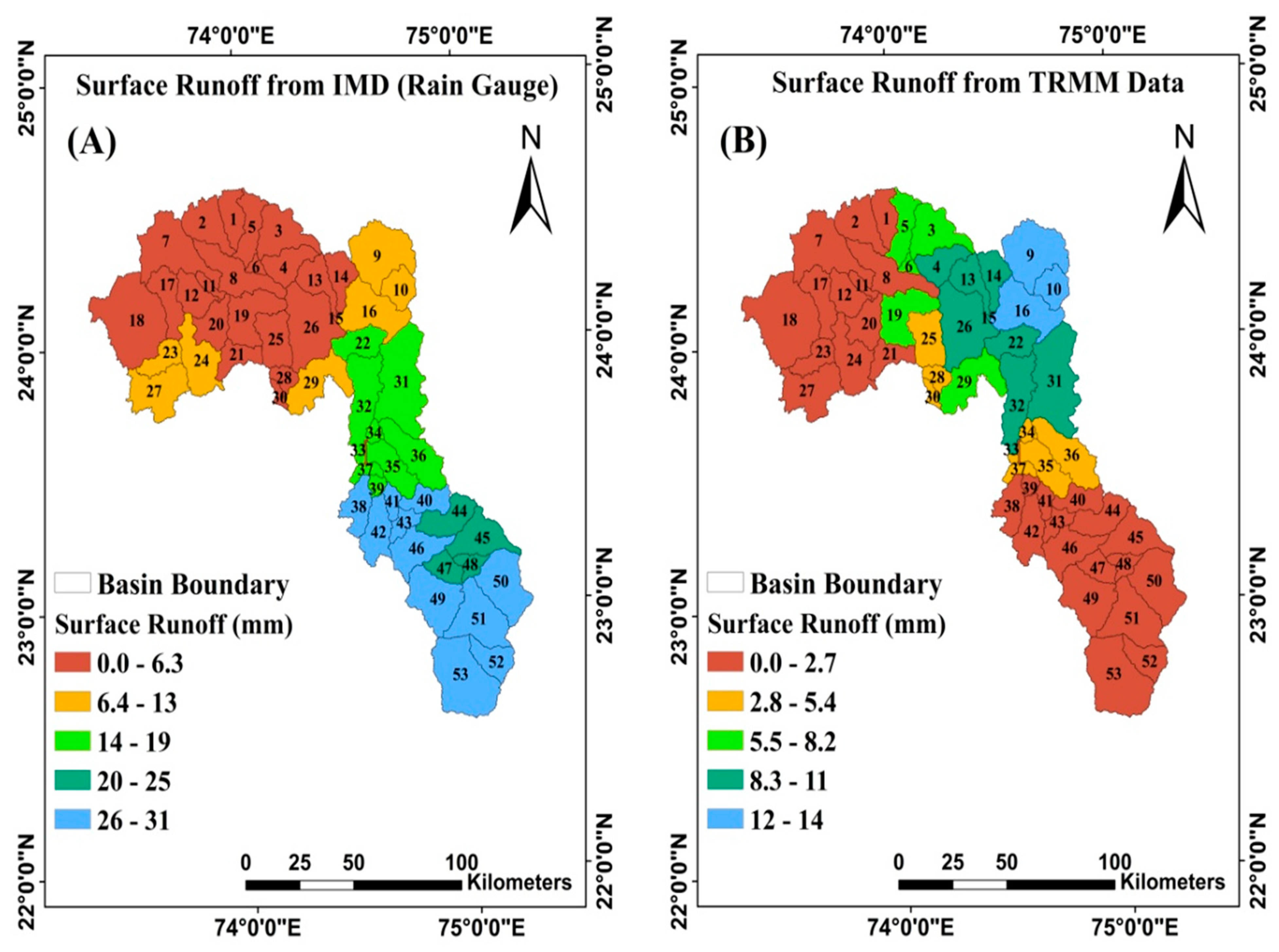
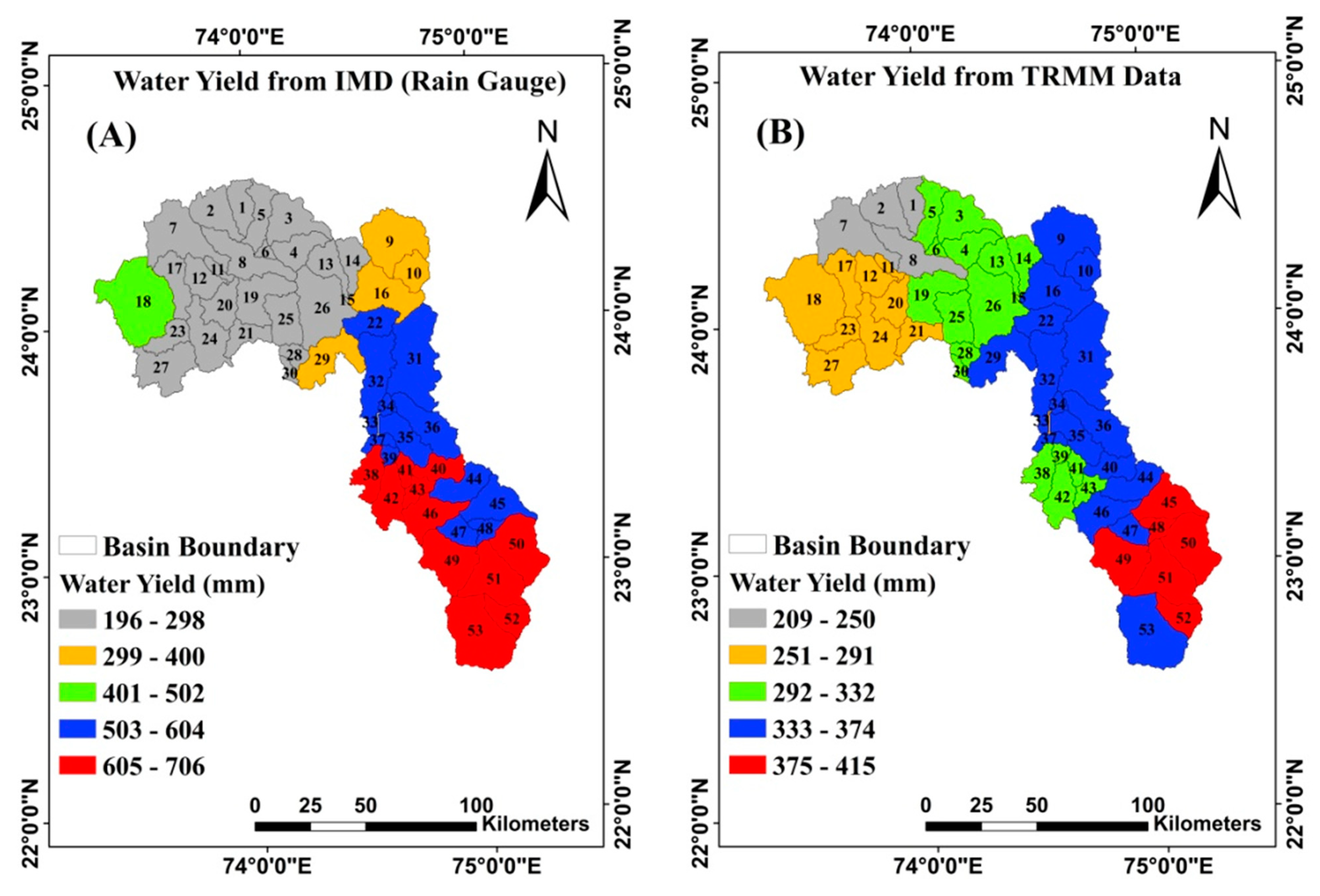
4.3. Intercomparison of IMD and TRMM Precipitation Impact on Hydrology

The TRMM 3B42 V7 daily precipitation data were used in a hydrological model to accomplish daily streamflow simulations at the Paderdibadi station. This station is located in Upper Mahi basin. During 1998–2001, the feasibility of TRMM precipitation on streamflow simulations in the Upper Mahi basin was assessed. Upper Mahi River basin data were calibrated for 1998–2000 and validated for 2001–2002.

Figure 8A shows that the IMD evapotranspiration value varies from 338 to 924 mm, with the lowest simulated value observed in the northern region of the Upper Mahi basin. In Figure 8B, the TRMM evapotranspiration value varies from 334 to 914 mm, with the lowest value observed in the northwest region of the basin. In Figure 8A,B, the IMD and TRMM data show that the highest simulated evapotranspiration is in the southern region of the Upper Mahi basin. Thus, higher evapotranspiration in the Mahi basin is due to the southern region with tropical wet climatic conditions.

In Figure 9A, the IMD precipitation value varies from 540 to 1200 mm, with the lowest precipitation observed in the northern regions of the Upper Mahi basin. By contrast, the highest precipitation was observed in the southeastern region of the basin. Figure 9B shows that the TRMM precipitation value varies from 550 to 790 mm. The lowest precipitation is observed in the northwestern region of the Upper Mahi basin and the most moderate precipitation in the southeastern region. The observed lowest precipitation in the northern region is caused by the subtropical wet climate, whereas the highest precipitation in the southern region results from the humid tropical weather.

In Figure 10A, the IMD surface runoff value varies from 0.0 to 31 mm, with the lowest runoff observed in the northern region of the Upper Mahi basin. By contrast, the highest surface runoff was observed in the southeastern region of the basin. In Figure 10B, the TRMM surface runoff value varies from 0.0 to 14 mm, with the lowest surface runoff observed in the northwestern and southern regions of the Upper Mahi basin, and the highest surface runoff was observed in the southeastern region. Surface runoff is directly proportional to rainfall intensity. The most increased surface runoff was observed in the southeastern region, which is also the region with the highest precipitation, according to the result shown in Figure 9. By contrast, the lowest surface runoff was observed in the northern region, which is the region with the most moderate precipitation according to the result shown in Figure 9.

In Figure 11A, the IMD water yield value varies from 196 to 706 mm, with the lowest water yield in the northern region of the basin and the highest water yield in the southeastern region. In Figure 11B, the TRMM water yield value varies from 209 to 415 mm, with the lowest water yield in the northern region of the Upper Mahi basin and the highest water yield in the southeastern region.

5. Conclusions

Satellite-derived products on the local and global scales have provided rainfall data to fill the data gap, particularly in a developing country with significant water scarcity. In this study, the performance of TRMM 3B42 V7 satellite rainfall products was investigated through a comparison with rain gauge data. The SWAT model was applied to simulate the streamflow of the Mahi River basin from 1998 to 2001 on a monthly scale. The model was calibrated and validated using SWAT-CUP, and the most sensitive parameters of the basin were found and ranked. In this analysis, the SUFI-2 algorithm was used to calibrate, validate, and find the sensitive parameters for the basin. The calibration and validation parameters belonged to the good categories and showed the good performance of the SWAT model in basin. The outcomes indicate that TRMM 3B42 V7 data are helpful for streamflow prediction and sensitivity analyses. TRMM 3B42 V7 is a monthly scale data used for Mahi basin streamflow prediction. These data show a strong correlation with the observed data. Additionally, the SWAT model can be employed to assess climate change and LULC impact on the Mahi River basin. Satellite-based precipitation estimations can provide vital information for estimating runoff using the SWAT hydrology model.

References

1. Almazroui, M.; Saeed, F.; Saeed, S.; Islam, M.N.; Ismail, M.; Klutse, N.A.B.; Siddiqui, M.H. Projected Change in Temperature and Precipitation Over Africa from CMIP6. Earth Syst. Environ. 2020, 4, 455–475. [Google Scholar] [CrossRef]
2. Council, N.R. NOAA’s Role in Space-Based Global Precipitation Estimation and Application; National Academies Press: Washington, DC, USA, 2007. [Google Scholar]
3. Clemens, M.; Bumke, K. A comparison of precipitation in-situ measurements and model predictions over the Baltic sea area. Phys. Chem. Earth Part B Hydrol. Oceans Atmosphere 2001, 26, 437–442. [Google Scholar] [CrossRef] [Green Version]
4. Valipour, M.; Bateni, S.; Sefidkouhi, M.G.; Raeini-Sarjaz, M.; Singh, V. Complexity of Forces Driving Trend of Reference Evapotranspiration and Signals of Climate Change. Atmosphere 2020, 11, 1081. [Google Scholar] [CrossRef]
5. Jensen, N.; Pedersen, L. Spatial variability of rainfall: Variations within a single radar pixel. Atmos. Res. 2005, 77, 269–277. [Google Scholar] [CrossRef]
6. Upadhyaya, S.; Ramsankaran, R. Review of Satellite Remote Sensing Data Based Rainfall Estimation Methods. Proceedings of HYDRO 2013 INTERNATIONAL, Chennai, India, 4–6 December 2013. [Google Scholar]
7. Tapiador, F.J.; Turk, F.; Petersen, W.; Hou, A.Y.; García-Ortega, E.; Machado, L.A.; Angelis, C.F.; Salio, P.; Kidd, C.; Huffman, G.J.; et al. Global precipitation measurement: Methods, datasets and applications. Atmos. Res. 2012, 104–105, 70–97. [Google Scholar] [CrossRef]
8. Kummerow, C.; Barnes, W.; Kozu, T.; Shiue, J.; Simpson, J. The Tropical Rainfall Measuring Mission (TRMM) Sensor Package. J. Atmos. Ocean. Technol. 1998, 15, 809–817. [Google Scholar] [CrossRef]
9. Ebert, E.; Janowiak, J.E.; Kidd, C. Comparison of Near-Real-Time Precipitation Estimates from Satellite Observations and Numerical Models. Bull. Am. Meteorol. Soc. 2007, 88, 47–64. [Google Scholar] [CrossRef] [Green Version]
10. Fereidoon, M.; Koch, M.; Brocca, L. Predicting Rainfall and Runoff Through Satellite Soil Moisture Data and SWAT Modelling for a Poorly Gauged Basin in Iran. Water 2019, 11, 594. [Google Scholar] [CrossRef] [Green Version]
11. Daneshvar, F.; Frankenberger, J.R.; Bowling, L.C.; Cherkauer, K.A.; Moraes, A.G.d.L. Development of Strategy for SWAT Hydrologic Modeling in Data-Scarce Regions of Peru. J. Hydrol. Eng. 2021, 26, 05021016. [Google Scholar] [CrossRef]
12. Tobin, K.J.; Bennett, M.E. Using SWAT to Model Streamflow in Two River Basins With Ground and Satellite Precipitation Data. JAWRA J. Am. Water Resour. Assoc. 2009, 45, 253–271. [Google Scholar] [CrossRef]
13. Li, D.; Christakos, G.; Ding, X.; Wu, J. Adequacy of TRMM satellite rainfall data in driving the SWAT modeling of Tiaoxi catchment (Taihu lake basin, China). J. Hydrol. 2018, 556, 1139–1152. [Google Scholar] [CrossRef]
14. Odusanya, A.E.; Mehdi, B.; Schürz, C.; Oke, A.O.; Awokola, O.S.; Awomeso, J.A.; Adejuwon, J.O.; Schulz, K. Multi-Site Calibration and Validation of SWAT with Satellite-Based Evapotranspiration in a Data-Sparse Catchment in Southwestern Nigeria. Hydrol. Earth Syst. Sci. 2019, 23, 1113–1144. [Google Scholar] [CrossRef] [Green Version]
15. Lal, P.; Prakash, A.; Kumar, A. Google Earth Engine for concurrent flood monitoring in the lower basin of Indo-Gangetic-Brahmaputra plains. Nat. Hazards 2020, 104, 1947–1952. [Google Scholar] [CrossRef] [PubMed]
16. Lal, P.; Prakash, A.; Kumar, A.; Srivastava, P.K.; Saikia, P.; Pandey, A.; Srivastava, P.; Khan, M. Evaluating the 2018 extreme flood hazard events in Kerala, India. Remote. Sens. Lett. 2020, 11, 436–445. [Google Scholar] [CrossRef]
17. Huffman, G.J.; Adler, R.F.; Stocker, E.; Bolvin, D.T.; Nelkin, E.J. Analysis of TRMM 3-Hourly Multi-Satellite Precipitation Estimates Computed in Both Real and Post-Real Time. In Proceedings of the 12th Conference on Satellitle Merorology and Oceanography, Long Beach, CA, USA, 9–13 February 2003. [Google Scholar]
18. Spruill, C.A.; Workman, S.R.; Taraba, J.L. Simulation of daily and monthly stream discharge from small watersheds using the swat model. Trans. ASAE 2000, 43, 1431–1439. [Google Scholar] [CrossRef]
19. Dos Santos, J.Y.G.; da Silva, R.M.; Neto, J.G.C.; Montenegro, S.M.G.L.; Santos, C.; Silva, A.M. Assessment of land-use change on streamflow using GIS, remote sensing and a physically-based model, SWAT. In Proceedings of the International Association of Hydrological Sciences; Copernicus GmbH: IAHS & Agrocampus Ouest, France, 2014; Volume 364, pp. 38–43. [Google Scholar]
20. Epelde, A.M.; Cerro, I.; Sanchez-Perez, J.M.; Sauvage, S.; Srinivasan, R.; Antiguedad, I. Application of the SWAT model to assess the impact of changes in agricultural management practices on water quality. Hydrol. Sci. J. 2015, 60, 1–19. [Google Scholar] [CrossRef]
21. Ligaray, M.; Kim, H.; Sthiannopkao, S.; Lee, S.; Cho, K.H.; Kim, J.H. Assessment on Hydrologic Response by Climate Change in the Chao Phraya River Basin, Thailand. Water 2015, 7, 6892–6909. [Google Scholar] [CrossRef]
22. Liu, J.; Zhang, C.; Kou, L.; Zhou, Q. Effects of Climate and Land Use Changes on Water Resources in the Taoer River. Adv. Meteorol. 2017, 2017, 1–13. [Google Scholar] [CrossRef] [Green Version]
23. Gosain, A.K.; Rao, S.; Basuray, D. Climate Change Impact Assessment on Hydrology of Indian River Basins. Curr. Sci. 2006, 90, 346–353. [Google Scholar]
24. Singh, A.; Gosain, A.K.; Singh, A.; Gosain, A.K. Climate-change impact assessment using GIS-based hydrological modelling. Water Int. 2011, 36, 386–397. [Google Scholar] [CrossRef]
25. Dubey, S.K.; Sharma, D.; Babel, M.S.; Mundetia, N. Application of hydrological model for assessment of water security using multi-model ensemble of CORDEX-South Asia experiments in a semi-arid river basin of India. Ecol. Eng. 2020, 143, 105641. [Google Scholar] [CrossRef]
26. Tobin, K.J.; Bennett, M.E. Temporal analysis of Soil and Water Assessment Tool (SWAT) performance based on remotely sensed precipitation products. Hydrol. Process. 2012, 27, 505–514. [Google Scholar] [CrossRef]
27. Tuo, Y.; Duan, Z.; Disse, M.; Chiogna, G. Evaluation of precipitation input for SWAT modeling in Alpine catchment: A case study in the Adige river basin (Italy). Sci. Total Environ. 2016, 573, 66–82. [Google Scholar] [CrossRef] [PubMed] [Green Version]
28. Chao, L.; Zhang, K.; Yang, Z.-L.; Wang, J.; Lin, P.; Liang, J.; Li, Z.; Gu, Z. Improving flood simulation capability of the WRF-Hydro-RAPID model using a multi-source precipitation merging method. J. Hydrol. 2021, 592, 125814. [Google Scholar] [CrossRef]
29. Wehbe, Y.; Temimi, M.; Weston, M.; Chaouch, N.; Branch, O.; Schwitalla, T.; Wulfmeyer, V.; Zhan, X.; Liu, J.; Al Mandous, A. Analysis of an extreme weather event in a hyper-arid region using WRF-Hydro coupling, station, and satellite data. Nat. Hazards Earth Syst. Sci. 2019, 19, 1129–1149. [Google Scholar] [CrossRef] [Green Version]
30. Zhang, Z.; Arnault, J.; Wagner, S.; Laux, P.; Kunstmann, H. Impact of Lateral Terrestrial Water Flow on Land-Atmosphere Interactions in the Heihe River Basin in China: Fully Coupled Modeling and Precipitation Recycling Analysis. J. Geophys. Res. Atmos. 2019, 124, 8401–8423. [Google Scholar] [CrossRef]
31. Yucel, I.; Onen, A.; Yilmaz, K.; Gochis, D. Calibration and evaluation of a flood forecasting system: Utility of numerical weather prediction model, data assimilation and satellite-based rainfall. J. Hydrol. 2015, 523, 49–66. [Google Scholar] [CrossRef] [Green Version]
32. Camera, C.; Bruggeman, A.; Zittis, G.; Sofokleous, I.; Arnault, J. Simulation of extreme rainfall and streamflow events in small Mediterranean watersheds with a one-way-coupled atmospheric–hydrologic modelling system. Nat. Hazards Earth Syst. Sci. 2020, 20, 2791–2810. [Google Scholar] [CrossRef]
33. Jain, S.K.; Agarwal, P.K.; Singh, V.P. Tapi, Sabarmati and Mahi Basins. In Hydrology and Water Resources Of India; Springer: Berlin/Heidelberg, Germany, 2007; pp. 561–595. [Google Scholar]
34. Mondal, D.P.; Gupta, R.K.; Beniwal, R.K.; Singh, T.; Singh, J.; Singh, B.; Dutt, B.; Kaur, H.; Chand, G. Integrated Hydrological Data Book; Central Water Commission: New Delhi, India, 2012. [Google Scholar]
35. Arnold, J.G.; Srinivasan, R.; Muttiah, R.S.; Williams, J.R. Large area hydrologic modeling and assessment part i: Model development. JAWRA J. Am. Water Resour. Assoc. 1998, 34, 73–89. [Google Scholar] [CrossRef]
36. Arnold, J.G.; Moriasi, D.N.; Gassman, P.W.; Abbaspour, K.C.; White, M.J.; Srinivasan, R.; Santhi, C.; Harmel, R.D.; van Griensven, A.; Van Liew, M.W.; et al. SWAT: Model Use, Calibration, and Validation. Trans. ASABE 2012, 55, 1491–1508. [Google Scholar] [CrossRef]
37. Dile, Y.T.; Karlberg, L.; Daggupati, P.; Srinivasan, R.; Wiberg, D.; Rockström, J. Assessing the Implications of Water Harvesting Intensification on Upstream–Downstream Ecosystem Services: A Case Study in the Lake Tana Basin. Sci. Total. Environ. 2016, 542, 22–35. [Google Scholar] [CrossRef]
38. Abbaspour, K.C.; Rouholahnejad, E.; Vaghefi, S.; Srinivasan, R.; Yang, H.; Kløve, B. A Continental-Scale Hydrology and Water Quality Model for Europe: Calibration and Uncertainty of a High-Resolution Large-Scale SWAT Model. J. Hydrol. 2015, 524, 733–752. [Google Scholar] [CrossRef] [Green Version]
39. Yang, X.; Liu, Q.; Fu, G.; He, Y.; Luo, X.; Zheng, Z. Spatiotemporal patterns and source attribution of nitrogen load in a river basin with complex pollution sources. Water Res. 2016, 94, 187–199. [Google Scholar] [CrossRef] [Green Version]
40. Yang, X.; Warren, R.; He, Y.; Ye, J.; Li, Q.; Wang, G. Impacts of climate change on TN load and its control in a River Basin with complex pollution sources. Sci. Total. Environ. 2018, 615, 1155–1163. [Google Scholar] [CrossRef] [Green Version]
41. Sahu, M.; Lahari, S.; Gosain, A.; Ohri, A. Hydrological Modeling of Mahi Basin Using SWAT. J. Water Resour. Hydraul. Eng. 2016, 5, 68–79. [Google Scholar] [CrossRef]
Figure 1. Study area map with the gauge station and TRMM grid points.
Sustainability 13 07560 g001
Figure 2. Input data in the model (A) land use, (B) soil, (C) DEM, and (D) sub-basin and stream network map.
Sustainability 13 07560 g002
Figure 3. Flowchart of the methodology.
Sustainability 13 07560 g003
Figure 4. Line plots for monthly rain gauge and TRMM data for the calibration period.
Sustainability 13 07560 g004
Figure 5. Line plots for monthly rain gauge and TRMM data for the validation period.
Sustainability 13 07560 g005
Figure 6. Calibration scatter plot for monthly TRMM observed and simulated streamflow (1998–1999) at the final catchment outlet Paderdibadi-30 Upper Mahi basin.
Sustainability 13 07560 g006
Figure 7. Validation scatter plot for monthly TRMM observed and simulated streamflow (2000–2001) at the final catchment outlet Paderdibadi-30 Upper Mahi basin.
Sustainability 13 07560 g007
Figure 8. Evapotranspiration determined using (A) IMD (rain gauge) and (B) TRMM data for the Upper Mahi basin during the period 1998–2001.
Sustainability 13 07560 g008
Figure 9. Precipitation determined using (A) IMD (rain gauge) and (B) TRMM data for the Upper Mahi basin during the period 1998–2001.
Sustainability 13 07560 g009
Figure 10. Surface runoff determined using (A) IMD (rain gauge) and (B) TRMM data for the Upper Mahi basin during the period 1998–2001.
Sustainability 13 07560 g010
Figure 11. Water yield determined using (A) IMD (rain gauge) and (B) TRMM data for the Upper Mahi basin during the period 1998–2001.
Sustainability 13 07560 g011