Reducing Socioeconomic Inequalities in the European Union in the Context of the 2030 Agenda for Sustainable Development

Abstract

The paper analyzes selected indicators monitoring the socioeconomic conditions of the European Union with regard to reducing inequalities. The main attention is paid to the 2030 Agenda and its Sustainable Development Goal 10, which calls for reducing inequalities within and among countries. The empirical part of the study is based on two separate studies and the data source is Eurostat. The first study focuses on the dynamics of the SDG10 indicators for the EU27. Due to the limited availability of all SDG10 indicators, the timeframe of this study covers the years 2010–2019. As a result, the SDG10 indicators for the EU27 as a whole are analyzed over that period or via a comparison of disparities between the two extreme dates, i.e., between 2010 and 2019. The second study focuses on the analysis of (dis)similarities of 27 individual European Union member states with respect to a set of variables capturing the socioeconomic conditions of these countries. The method used is cluster analysis, supported by the linear ordering method and principal component analysis. Due to the limited availability of indicators measuring the progress towards SDG10, especially those related to the evaluation of a citizenship gap, the second research does not use all indicators directly assigned to SDG10 (because most of them are not available for all countries), but rather employs a set of additional variables that may potentially affect the levels and dynamics of inequalities among and within countries. The general conclusion of the study is that the analysis of SDG10 indicators over the medium term (i.e., over the period 2010–2019) implies that the EU27 was able to make progress in reducing inequalities among countries; however, the income inequalities within countries persist or have even deepened. The insights from multivariate statistical methods emphasize the existing disparities between a group of countries, including Spain, Bulgaria, and Romania, and the rest of the EU countries in both analyzed years (i.e., in 2010 and 2019), regardless of the set of variables applied in analyses. Moreover, the results highlight the persistence in disparities between “old” and “new” member states and suggest the disparity between the “peripheral” and the rest of the “old” EU countries. Furthermore, the role of expenditure on social protection in affecting income disparities is emphasized, as is the impact of demographic factors in emphasizing the differences in socioeconomic situations across EU member states.

1. Introduction

The 2030 Agenda for Sustainable Development and its 17 Sustainable Development Goals (SDGs) call for nations to become more sustainable, ensuring the social inclusion of all. The Agenda is a global action plan for building resilient societies and promoting sustainable development. In particular, SDG10 of the Agenda aims to reduce inequalities among and within countries in many dimensions, mainly those related to income but also those related to age, race, disability, sex, origin, religion, economic status, etc. The importance of that goal arises from the fact that large disparities negatively affect sustainable development and slow down progress towards achieving the rest of the SDGs. The latter conclusion resulted from the fact that progress made in achieving one goal impacts the outcomes of other goals. In this context the 2030 Agenda expresses the interlinked nature of SDGs [1]. Moreover, the large scale of inequalities hampers social cohesion and reduces equal access to education and health services or negatively impacts social inclusion.

The motivation of the study is related to analysis of the selected socioeconomic variables that may affect the progress in reducing inequalities in the EU. Moreover, the study shows an attempt to analyze the (dis)similarities of the EU countries with respect to the variables to assess the progress of these countries with regard to SDG10 of the 2030 Agenda. The need for such analysis is confirmed in the literature. Many studies analyze the similarities of EU or OECD countries concerning the different SDGs or different strategies. The progress towards achieving the targets of the Europe 2020 Strategy has been studied by, for example, [2,3,4,5,6,7]. These papers offer different multivariate methods to support the recognition of the paths and to formulate conclusions, including, among others, cluster analysis [5,6] or by building rankings of analyzed countries see, e.g., [3]. The performance of the SDGs or selected components has been analyzed by [8,9,10,11]. Many studies consider the general performance of the SDGs, including a large set of indicators applied for a group of countries see, e.g., [9] using multivariate methods. Some studies analyze single countries, an example of which is [10], who focus on the case of Spain. The conclusion is that Spain requires urgent policies in order to fulfill the standards in sustainability by the year 2030. The study in [12] provides an interesting analysis of the Spanish synergies and trade-offs among the SDGs, calculating the correlation between a reduced set of indicators representing each SDG. The empirical results make it possible to conclude that almost 80% of the significant interactions can be classified as synergies or trade-offs. The EU labor market inequalities, reflected by the specific indicators proposed for Sustainable Development Goal 8, are analyzed by, e.g., [13]. A similar analysis, presented in [14], concerns the role of the SDGs from the point of view of targets aimed at health and well-being.

Despite this, there is a lack of similar analyses of SDG10, even though that SDG plays an important role in the structure of the Agenda. It seems that the difficulties in providing similar analyses may be a result of the limited access and availability of all SDG10 indicators at a country-specific level. As a result, in this paper, the list of available SDG10 indicators is extended by a set of variables that may affect the levels and dynamics of inequalities among and within countries. Thus, the similarities of countries are analyzed on the basis of an alternative set of variables to the set consisting of only SDG10 indicators.

Considering the motivation, the goal of the study is twofold. Firstly, the aim of the study is to assess the dynamics of the EU27 with regard to SDG10 by analyzing appropriate indicators attributed to that SDG. Secondly, the paper investigates the (dis)similarities of the EU countries with respect to the variables that may affect the levels of the inequalities or the progress towards reducing these inequalities. Due to the limited availability of SDG10 indicators at a country-specific level, the analysis (under this goal) is prepared through the use of an alternative set of variables monitoring the socioeconomic conditions of the economies. In order to achieve the goal, multivariate statistical methods are applied. The methods include cluster analysis and the linear ordering method, supplemented by the principal component analysis (PCA). All data derive from Eurostat, and the timeframe (due to data availability for all 27 countries) covers the period 2010–2019. The contribution and novelty of the study are also supported by the analysis of the progress in achieving SDG10 in the EU context in the medium-term and its wider linkage with the socioeconomic conditions of the EU economies using multivariate methods, including cluster analysis, linear ordering and built ranking of countries, and PCA.

The structure of the paper is as follows. The next section provides general information on the origins of the 2030 Agenda and the importance of SDG10. The third section presents insights derived from an analysis of the SDG10 indicators related to three dimensions of the sustainable goal. Thereafter, the data and the methods of multivariate analysis are presented, while in the fifth section the results are presented. The sixth section provides the discussion, while the last section presents the general conclusions.

2. The 2030 Agenda and Sustainable Development Goal 10—Reduce Inequality within and among Countries

In 2015, the United Nations General Assembly adopted the document of the post-2015 development agenda: “Transforming our world: The 2030 Agenda for Sustainable Development” [15]. The preamble of the document outlines that the Agenda is an ambitious plan of actions aimed at achieving sustainable development by means of improvement in areas related to people, the planet, prosperity, peace and partnership [15]. The integral element of the 2030 Agenda is that of a set of 17 Sustainable Development Goals (SDGs) and 169 targets, which were adopted during the UN Summit in September 2015 by all United Nations member states. As assumed in [15], successful realization of the SDGs will impact everyone and transform the world into a better place. The timeframe for achieving a meaningful improvement was set at 15 years (i.e., by 2030). The aforementioned integrated goals of the SDGs are assigned to the following areas: SDG1—End poverty in all its forms everywhere; SDG2—End hunger, achieve food security and improved nutrition and promote sustainable agriculture; SDG3—Ensure healthy lives and promote well-being for all at all ages; SDG4—Ensure inclusive and equitable quality education and promote lifelong learning opportunities for all; SDG5—Achieve gender equality and empower all women and girls; SDG6—Ensure availability and sustainable management of water and sanitation for all; SDG7—Ensure access to affordable, reliable, sustainable and modern energy for all; SDG8—Promote sustained, inclusive and sustainable economic growth, full and productive employment and decent work for all; SDG9—Build resilient infrastructure, promote inclusive and sustainable industrialization and foster innovation; SDG10—Reduce inequality within and among countries; SDG11—Make cities and human settlements inclusive, safe, resilient and sustainable; SDG12—Ensure sustainable consumption and production patterns; SDG13—Take urgent action to combat climate change and its impacts; SDG14—Conserve and sustainably use the oceans, seas and marine resources for sustainable development; SDG15—Protect, restore and promote sustainable use of terrestrial ecosystems, sustainably manage forests, combat desertification, and halt and reverse land degradation and halt biodiversity loss; SDG16—Promote peaceful and inclusive societies for sustainable development, provide access to justice for all and build effective, accountable and inclusive institutions at all levels; SDG17—Strengthen the means of implementation and revitalize the global partnership for sustainable development. The SDGs derive from experience related to the realization of the Millennium Development Goals because the SDGs were built upon the Millennium Development Goals adopted in 2000 by the United Nations General Assembly in the outline declaration entitled the United Nations Millennium Declaration [16]. The deadline for reaching the targets of the eight Millennium Development Goals was set at 2015; thus, the SDGs are elements of a new plan set for the 15 years following the previous deadline for the Millennium Development Goals global action plan. In order to analyze the progress made in achieving the SDGs, there is a need for monitoring the realization of the targets. For this purpose, the UN launched the High-level Political Forum on Sustainable Development (which is responsible for reviewing the 2030 Agenda at the global level). It was mandated in 2012 via the document of the United Nations Conference on Sustainable Development (Rio + 20), i.e., “The Future We Want” see [17], whereas the organizational issues are outlined in General Assembly Resolution 7/290 see [18]. The UN Conference on Sustainable Development (Rio + 20) was an important milestone in building the frameworks of the Agenda. Additional arrangements concerning following up on and reviewing the Agenda at the global level are outlined in General Assembly Resolution 70/290 see [19]. As a result, in order to measure the progress towards achieving the SDGs, a set of indicators were designed and adopted (list of 232 indicators) in July 2017 by the United Nations General Assembly in Resolution 71/313 see [20]. These indicators were developed by the Inter-agency and Expert Group on Sustainable Development Goal Indicators [20]. Resolution 71/313 defines the indicators for each goal and target of the Agenda [20, Annex]. The Resolution [20] assumes that indicators will be reviewed comprehensively by the Statistical Commission during its 51st session (in 2020) and 56th session (in 2025). The indicator list revised in 2020 is built from 231 different indicators (the global indicator framework for the SDGs includes 247 indicators due to 12 indicators being repeated under more than one different target)—see [21]. The assessment of trends in the indicators against the targets defined for each SDG allows analyzing the progress made in achieving the goals of the 2030 Agenda.

In the case of the EU, the progress towards the SDGs is regularly monitored by Eurostat on the basis of the set of EU SDG indicators. In the EU context, the set for the 17 SDGs comprises 100 indicators, but 36 of them are multipurpose (used to monitor more than one SDG). Generally, Eurostat proposes monitoring each goal via six indicators primarily attributed to the SDG, except for SDG14 and SDG17—both of which have only five attributed indicators [22].

In this study, special attention is paid to Sustainable Development Goal 10 (which calls for reducing inequalities within and among countries). Detailed information on the targets and indicators attributed to SDG10 is presented in

Table 1. Targets and indicators announced for SDG10. Source: own work based on [20,23].

Target	Indicators
10.1 By 2030, progressively achieve and sustain income growth of the bottom 40 per cent of the population at a rate higher than the national average	10.1.1 Growth rates of household expenditure or income per capita among the bottom 40 per cent of the population and the total population
10.2 By 2030, empower and promote the social, economic and political inclusion of all, irrespective of age, sex, disability, race, ethnicity, origin, religion or economic or other status	10.2.1 Proportion of people living below 50 per cent of median income, by sex, age and persons with disabilities
10.3 Ensure equal opportunity and reduce inequalities of outcome, including by eliminating discriminatory laws, policies and practices and promoting appropriate legislation, policies and action in this regard	10.3.1 Proportion of population reporting having personally felt discriminated against or harassed in the previous 12 months on the basis of a ground of discrimination prohibited under international human rights law
10.4 Adopt policies, especially fiscal, wage and social protection policies, and progressively achieve greater equality	10.4.1 Labor share of GDP, comprising wages and social protection transfers
10.5 Improve the regulation and monitoring of global financial markets and institutions and strengthen the implementation of such regulations	10.5.1 Financial Soundness Indicators
10.6 Ensure enhanced representation and voice for developing countries in decision-making in global international economic and financial institutions in order to deliver more effective, credible, accountable and legitimate institutions	10.6.1 Proportion of members and voting rights of developing countries in international organizations
10.7 Facilitate orderly, safe, regular and responsible migration and mobility of people, including through the implementation of planned and well-managed migration policies	10.7.1 Recruitment cost borne by employee as a proportion of monthly income earned in country of destination. 10.7.2. Number of countries that have implemented well-managed migration policies
10.a Implement the principle of special and differential treatment for developing countries, in particular least developed countries, in accordance with World Trade Organization agreements	10.a.1 Proportion of tariff lines applied to imports from least developed countries and developing countries with zero-tariff
10.b Encourage official development assistance and financial flows, including foreign direct investment, to States where the need is greatest, in particular least developed countries, African countries, small island developing States and landlocked developing countries, in accordance with their national plans and programs	10.b.1 Total resource flows for development, by recipient and donor countries and type of flow (e.g., official development assistance, foreign direct investment and other flows)
10.c By 2030, reduce to less than 3 per cent the transaction costs of migrant remittances and eliminate remittance corridors with costs higher than 5 per cent	10.c.1 Remittance costs as a proportion of the amount remitted

below.

The SDG10 is attributed to the prosperity area of the 2030 Agenda [24]. SDG10 has 10 important targets and their realization is monitored via the use of indicators originally presented in UNGA Resolution 71/313. Taking into account the ambition of the 2030 Agenda, SDG10 calls for reducing inequalities and promoting the political, social and economic inclusion of all. The goal strongly focuses on ensuring sustainable development (which is assumed to be inclusive, more equal, and resilient to unexpected changes and events). The progress towards transforming the world into one that is more equal affects the actions taken to reduce inequalities in many dimensions, including income, age, gender, ethnicity, religion, and others, such as a reduction in between-country inequalities and within-country inequalities. Furthermore, an important issue is related to migration and migrants, particularly the 2030 Agenda and the SDG10 aim of ensuring the facilitation of safe migration. As a result, SDG10 focuses on reducing inequalities within and among countries and encompasses a strong orientation towards the social inclusion of all.

The importance of SDG10 increased in the context of the COVID-19 pandemic. This is due to the fact that, on the one hand, the pandemic has deepened inequalities, especially in the socioeconomic context; on the other hand, existing inequalities and those that have not been eliminated have amplified the negative effects of the pandemic. The United Nations emphasize that the most vulnerable groups of people being hit the hardest by the pandemic are older persons, persons with disabilities, children, women, migrants, and refugees [25].

3. Inequalities in the European Union—A Quick Look at Currently Available Data

This section illustrates selected dimensions of the socioeconomic position of the EU27, analyzed from the point of view of the dynamics of the SDG10 indicators and other variables that may affect the progress towards achieving SDG10.

3.1. The Analysis of SDG10 Indicators

SDG10 aims to reduce inequalities as analyzed in three dimensions—inequalities between countries, inequalities within countries, and via the progress made in facilitating migration and social inclusion. The three areas and their indicators are as follows:

• Monitoring of reduction of inequalities between countries (indicators: purchasing power adjusted GDP per capita; adjusted gross disposable income of households per capita);
• Monitoring of reduction of inequalities within countries (indicators: income distribution (quintile share ratio); relative median at-risk-of-poverty gap (% of distance to poverty threshold); income share of the bottom 40% of the population (% of income); people at risk of poverty or social exclusion by degree of urbanization (% of population));
• Monitoring facilitation in the field of migration and social inclusion (indicators: asylum applications by state of procedure (number per million inhabitants); people at risk of income poverty after social transfers, by citizenship (% of population aged 18 years or above); young people neither in employment nor in education and training (NEET), by citizenship (% of population aged 15 to 29); early leavers from education and training, by citizenship (% of population aged 18 to 24); employment rate, by citizenship (% of population aged 20 to 64)).

The analysis of Eurostat’s indicators allows assessing the progress of the EU in eliminating these inequalities. It is important because having equal opportunities for all strengthens the progress made in achieving sustainable development. As a result, the analysis presented below focuses on a set of indicators which reflect the status of the 27 European Union countries and the dynamics of the selected indicators assigned to monitor SDG10. The observation of trends outlines the progress of the EU27 with regard to the targets of SDG10 as presented in Table 1.

The indicators published by Eurostat are presented for individual countries or as indicators for the EU27 as a whole. The indicators published for the EU27 make it possible to outline general trends. However, most of the SDG10 indicators for individual countries are available in different timeframes. The assessment of the availability of all indicators implies that most of them are available for the timeframe of 2010–2019. This observation has affected the decision regarding the selected indicators monitoring SDG10 being presented, including the timeframe. As a result, the data allows comparing changes over the years 2010 and 2019 and formulating some conclusions with regard to the medium-term trends in achieving SDG10 at the aggregated EU27 level.

3.1.1. Inequalities between Countries

In the context of SDG10 the scale of inequalities between countries is monitored via two types of indicators based on income. The first indicator aims at disparities in GDP per capita, while the second one focuses on disparities in disposable household income per capita. The general indicator for EU27 GDP per capita is calculated by Eurostat as the coefficient of variation of national figures which are based on the GDP per capita expressed in purchasing power standards (PPS). The use of PPS eliminates the differences in price levels between countries and, as a result, ensures more adequate comparisons of trends in GDP (in volumes). The coefficient of variation is a relative measure of variability, and a decrease in the coefficient informs of a decrease in dispersion in the variable analyzed. Figure 1 presents data for the EU27 and the euro area.

Over the period 2010–2019 the coefficient for the EU27 declined by 1.5 percentage points (p.p.), whereas for the EA19 it increased by 0.9 p.p. The increase in disparity is observed mainly over the years 2013–2015 (the post-crisis period). The disparities between these two groups of countries were diminishing over the period until 2018. In 2019 the variability of GDP per capita in PPS was slightly higher in the eurozone countries than in the EU27. The detailed analysis of the data for individual countries is based on an index under the assumption that the EU27 is set to 100. The figure below (Figure 2) shows the index for individual countries. The index is useful for a cross-country comparison in a given year. However, because of the interest in comparing changes in the positions of the 27 countries between the years 2010 and 2019, the figure includes the indicator for these two years. As presented, the inequalities between the EU27 countries are still visible.

In 2010, 15 out of the current EU27 countries were below the index of 100, while in 2019 there were 16 EU countries. The highest value of the index in both years was for Luxembourg, for which in 2010 and 2019 the calculated index of GDP per capita in PPS stood at approximately 260. The lowest position in both years was observed for Bulgaria (the index in 2010 was only 44, and in 2019 was 53). Generally, 10 “old” EU countries maintained a position above the baseline index of 100 in each of the years analyzed. Figure 2 suggests that income inequalities between countries continue to persist in the EU. Moreover, there is a visible division of the EU into Eastern and Western EU countries, as well as into “old” and “new” EU countries.

Consideration of inequalities in the adjusted gross disposable income of households and non-profit institutions serving households (NPISH) via the use of an adequate index calculated by Eurostat in relation to the EU27 average set at 100 implies that the maintenance of inequalities is also observable (see Figure 3). Despite the fact that data for 2019 are not available for Bulgaria and Luxembourg, as well as for Malta (Malta does not report these data in the Eurostat database), disparities between the “old” and “new” EU countries and between the “peripheral” countries of the “old” EU (Portugal, Greece, Spain) and the rest of the “old” EU countries still remain.

In the case of individual countries, for the year 2010, indices are available for 26 countries (data are lacking for Malta), and in 2019 for 24 countries (data are lacking for Malta, as well as for Bulgaria and Luxembourg). As presented, in general the index was higher in 2019 than in 2010 for the “new” EU countries, whereas in the case of “old” Europe the index was lower in 2019 (except for Germany, for which the index was higher, and for Denmark and Finland, whose index value was the same in both years). Thus, the comparison of the index values may indicate, despite the lack of data for three countries in 2019, convergence of the “new” EU countries towards “old” Europe (as exhibited by a reduction in disparity measured by the index for the adjusted gross disposable income of households). The conclusion regarding the reduction of disparities is supported by the reduction of the distance (i.e., disparity in index) between “old” and “new” member states.

3.1.2. Inequalities within Countries

Figure 4 presents three panels with three indicators that support monitoring SDG10 in the context of within-country inequalities.

Eurostat calculates the relative median at-risk-of-poverty indicator as the distance between the median equivalized total net income of persons below the specified at-risk-of-poverty threshold and the at-risk-of-poverty threshold itself (the threshold is set at 60% of the national median equivalized disposable income of all people in a country and not for the EU as a whole), expressed as a percentage of the at-risk-of-poverty threshold see [26]. The indicator is presented in the upper-left panel of Figure 4. As illustrated, between 2010 and 2019 the value of the indicator increased by 1.4 p.p., denoting an increase in inequalities and, as a consequence, deterioration of the situation of the poor. The detailed analysis of country-specific data indicates that in 2019 the highest indicators were observed in Romania (poverty gap amounted to 33%), Italy (30%), Spain (29.1%), and Hungary (28.9%), while the lowest poverty gaps, i.e., the median income distance of people at risk of poverty from the poverty threshold, were observed in Czechia (14.1%), Ireland (14.8%), Finland (14.9%), and Cyprus (16%). Between 2010 and 2019 the indicator decreased in 16 countries and the size of the reduction ranges from −0.2 p.p. in Malta and Poland to −7 p.p. in Czechia. The increase in the poverty gap ranged from 0.9 p.p. in the Netherlands to 12.4 p.p. in Hungary. Generally, a higher ratio in 2019 than in 2010 denotes a deepening of existing income inequality and a higher poverty gap.

The upper-right panel of Figure 4 presents the indicator responsible for monitoring the income share of the EU27 (i.e., total disposable household income) received by the bottom 40% of the population. Although the change between the years 2010 and 2019 is zero, over the two years the index slightly diminished but generally was quite stable (the lowest value was observed in 2014 and 2015, i.e., 20.9%, denoting that 20.9% of the total income was earned by the bottom 40% of the EU population in those years). The third panel of Figure 4 shows the indicator measuring the inequality of income distribution, which is calculated by Eurostat as a ratio of the total income received by 20% of the population with the highest income (the top quintile) to that received by 20% of the population with the lowest income (the bottom quintile). The general change in the index for the EU27 between 2010 and 2019 is that of an increase of 0.1 units. At the domestic level the indicator increased in the case of 11 countries (the size of the increase ranges from 0.04 units in Cyprus to 2.24 units in Bulgaria) and decreased in 16 countries (from −0.03 units in Slovenia to −0.91 units in Lithuania). The highest values in 2019 were observed in Bulgaria (8.1) and Romania (7.08), and the lowest in Czechia and Slovakia (3.34). In 2019 the ratio in 10 countries was higher than the EU27 average, and in 2010 in 11 countries. In 2010 the highest value was 7.35 for Lithuania and the lowest (3.41) was observed for Hungary. Despite the slight increase in the indicator over the medium term, the analysis of Figure 4 informs of an increase of the income inequalities over that period. For example, in 2014 and 2015 the ratio was 5.22, denoting that income received by 20% of the “top” EU27 population was in the two years 5.22 times higher than that received by 20% of the population with the lowest income. Generally, all three panels of Figure 4 inform that the EU27 inequalities within countries increased over 2010–2015, but after 2015 they decreased, achieving in 2019 a level similar to in 2010.

The last indicator concerns the analysis of the risk of poverty or social exclusion, considered in the context of the degree of urbanization. The data for 2019 are presented in Figure 5.

In 2019 the highest risks of poverty or social exclusion analyzed for cities were observed in Belgium, Denmark, Germany, France, Italy, the Netherlands, Austria, and Slovenia—generally in the “old” EU countries. The highest risk in rural areas was noticed in 13 countries, whereas the highest was observed in Bulgaria and Romania. Generally, in 2019, for most of the EU countries the risk of poverty was higher in rural areas, but the average for the EU27 for each degree of urbanization was similar. Over the period 2010–2019 the average evaluation of the risk of poverty or social exclusion in the EU countries emphasizes a decrease. The EU27 indicator for cities decreased from 22.2% to 21.3%, for rural areas from 30.0% to 22.4%, and for towns and suburbs from 20.5% to 19.2%.

3.1.3. Inequalities Related to Facilitating Migration and Social Inclusion

Figure 6 presents the medium-term development of indicators describing social inclusion and migration aspects (analyzed from the point of view of citizenship). Due to the lack of availability of detailed data for all 27 individual EU countries, the figure shows general data for the EU27.

The informative value of the presented data is that between 2010 and 2019, the citizenship gap for the NEET rate and for early school leavers decreased. In 2010 the gap for the NEET rate was 14.5 p.p. and in 2019 it was 12.4 p.p. Despite the slight reduction in citizenship disparity in the NEET rate, the general overview of the indicators informs of an increasing trend. In 2010 the NEET rate for EU27 citizens was 14.5% and in 2019 was 15.1%. The increase (by 1 p.p.) was also observed in the case of non-EU27 citizens. Moreover, the NEET rate was generally more than two times higher in the case of non-EU27 citizens in the age group 15–29. Such disparity is also confirmed in the analysis of the indicator for early school leavers. Indeed, the citizenship gap decreased from 24.5 p.p. in 2010 to 18 p.p. in 2019, but the rate was around three times higher in the case of non-EU27 reporting countries. A positive aspect is that over 2010–2019, both analyzed groups experienced a decrease of the rate of early school leavers. In the case of EU27 reporting countries there was a reduction of 3.6 p.p., while in the group of non-EU27 citizens the reduction was that of 10.1 p.p. The employment rate increased in both groups over time, but the gap in the employment rate increased from 10.6 p.p. in 2010 to 13.8 p.p. in 2019 (to the disadvantage of non-EU citizens). The large inequality concerns the indicator for income poverty. Indeed, over time the indicator decreased in both groups; however, the citizenship gap for income poverty after social transfer increased from 23.1 p.p. in 2010 to 23.5 p.p. in 2019 (to the disadvantage of non-EU citizens).

Finally, the indicator for asylum applications is presented—see: Figure 7. In 2019, asylum applications accounted for 1371 per million inhabitants, while in 2010, first-time applications constituted around 418 per million inhabitants. Enormous amounts of asylum first-time applicants were registered in 2015 and 2016. This was a result of the migrant crisis that started in 2014, whose peak occurred over 2015–2016.

As presented, at the peak of the migration crisis, the number of first-time asylum seekers applying for international protection between 2014 and 2015 increased by more than 128.2%, while between 2016 and 2017 it decreased by around 46.9%. After a decline in the years 2016–2018, in 2019, in comparison to the previous year, the number of first-time applicants (per million inhabitants) increased by around 11.9%.

3.2. Beyond the SDG10 Indicators—Selected Aspects of Inequalities and Social Policy in the EU

A popular measure of income distribution inequality is the Gini coefficient (or Gini index). The indicator ranges between 0 and 1 (or, if multiplied by 100, between 0 and 100). A value of 0 denotes a homogenous distribution and it is understood to represent a situation in which all persons have the same income, whereas a value of 1 (or 100) represents when only one person in the population receives income. Thus, the higher the indicator, the higher the income distribution and, therefore, the greater the income inequalities.

In 2019 the average Gini coefficient for the EU27 was 30.2, which was the same in 2010. Over the period 2010–2019 it witnessed the highest value in 2014 (30.9). The analysis of the data for individual countries informs that in 2010 the highest value of the Gini coefficient was observed in Lithuania (37.0) and the lowest in Slovenia (23.8), whereas in 2019 the highest value was seen in Bulgaria (40.8) and the lowest in Slovakia (22.8). Over the period 2010–2019 the Gini index increased in 12 countries, mostly in Bulgaria (by 7.6 units), and decreased in 15 countries, mostly in Slovakia (−3.1 units). Figure 8 indicates how the size of the Gini index changed between 2010 and 2019.

Governments may use different tools to reduce inequalities, mainly redistributive fiscal policy based on taxation and transfer systems. One of the tools is that of spending on social protection. Taking into account the COFOG (i.e., Classification of the Functions of Government), spending on social protection comprises a large share of total spending of general government in the EU27. The share of the social protection function of governmental expenditure out of the total spending increased over 2010–2019 (by 2.3 p.p.), whereas its share in GDP decreased—in 2010, governmental social protection expenditure was 19.8% of GDP and in 2019 was 19.3%. In the EU member states, social protection was the most important function of total governmental expenditure. In 2019, governmental social protection expenditure in the EU27 was equivalent to 19.3% of GDP (see Figure 9), compared to 19.2% of GDP in 2018 and 19.8% in 2010. The share of social protection expenditure out of the total expenditure increased from 39.1% of the total expenditure in 2010 to 41.4% of the total expenditure in 2019.

Analyzing the data at the country level, the highest shares of social protection spending out of the total spending of general government were observed in 2019 in Finland (45.1%), Germany (43.7%), and Denmark and Italy (43.5%); and in 2010 in Denmark (43.8%), Finland (41.9%), and Germany (41.7%). In 2019, countries with high expenditure on social protection in relation to GDP comprised Finland (24%) and France (23.9%), with the lowest ratios being observed in Ireland (8.9%) and Malta (10.8%). In 2010 the highest shares of spending on social protection in GDP were seen in Denmark (24.8%), France (23.7%), and Finland (22.6%), with the lowest in Cyprus (12.1%), Bulgaria (12.9%), and Malta (13.3%). The comparison of the annual data makes it possible to conclude about the strong division of the EU countries, whose high spenders include Denmark, Finland, France, and Germany, among others, and whose low spenders are mainly “new” EU member states: Bulgaria, Romania, Cyprus, and Malta, but also Ireland, Greece, and Spain (i.e., peripheral countries).

Spending on social protection focuses on: sickness and disability, old age, survivors, family and children, unemployment, housing, social exclusion n.e.c., R&D social protection, and social protection n.e.c. The detailed analysis of the structure of EU27 spending on social protection indicates that it is driven mainly by the category “old age”. As a result,

Table 2. Population structure and aging in EU27. Source: own work based on Eurostat data.

	2010	2011	2012	2013	2014	2015	2016	2017	2018	2019	Change (p.p.) 2019–2010
Age dependency ratio	49.4	49.7	50.2	50.9	51.5	52.3	52.9	53.6	54.3	54.9	5.5
Old-age dependency ratio	26.3	26.6	27.1	27.7	28.3	29.0	29.6	30.2	30.8	31.4	5.1
Young-age dependency ratio	23.0	23.1	23.1	23.2	23.2	23.3	23.3	23.4	23.5	23.5	0.5
Proportion of population aged 0–14 years	15.4	15.4	15.4	15.4	15.3	15.3	15.3	15.2	15.2	15.2	−0.2
Proportion of population aged 65 years and more	17.6	17.8	18.0	18.3	18.7	19.0	19.3	19.7	20.0	20.2	2.6
Proportion of population aged 80 years and more	4.7	4.8	5.0	5.1	5.2	5.3	5.4	5.6	5.7	5.8	1.1

presents selected indicators describing population aging in the EU27.

As shown, in 2019, the age dependency ratio (i.e., the ratio of economically inactive people, i.e., below 15 years of age and aged 65 or above, to the number of people of working age, i.e., 15–64 years old) over the period 2010–2019 increased by 5.5 p.p. Table 2 suggests that the increase was mainly driven by the increase in the old-age dependency ratio (i.e., the ratio of the number of elderly people aged 65 or above to the number of people of working age, i.e., 15–64 years old). As presented, over the years 2010–2019 the increase of the share of elderly people aged 80 years or above out of the total population was higher than the change in the share of the population aged 0–14 out of the total population. Population aging in the EU is a very advanced process and affects many aspects of sustainable growth, policy implementation, and socioeconomic aspects. The phenomenon determines higher age-related spending and a need for the strongest efforts in finding sources of financing them. Moreover, aging may become a potential driver expanding the inequalities in the EU due to its impact on the income and the quality of life and well-being of the elderly.

4. Methods and Data—Empirical Analysis of the EU Countries

The aim of SDG10 is to achieve significant sustainable improvement in the quality of life, well-being, and socioeconomic situation of people all over the world by reducing inequalities. In this section an attempt to analyze the (dis)similarities of European Union countries with respect to the selected socioeconomic variables affecting SDG10 and its indicators is analyzed. The comparison allows for an assessment of the socioeconomic conditions of the EU member states considered, mainly via the implementation of the SDG10 indicators and analyzing the inequalities.

4.1. Methods

The previous section presents a general overview of the situation of the EU27 as a whole in the context of SDG10 and inequalities. The analysis of indicators confirms the existence of disparities. The aim of this section is to analyze and compare EU countries in the context of the development of SDG10 indicators and other socioeconomic variables and assess the potential (dis)similarities between the economies. That goal is achieved through the use of multivariate statistical methods, especially the hierarchical grouping method (which is a cluster analysis). Moreover, the ordering of countries with respect to the set of chosen variables is proposed as an additional supplementary analysis and it is presented in the form of ranking, where the approach used is Hellwing’s linear ordering method.

The advantage of the agglomeration technique is that it allows joining objects which are very similar into clusters. In general, the algorithm of cluster analysis is based on the analysis of the distance between objects [27], and the greater the distance between objects, the lower the level of similarity that they exhibit. As a consequence, an important step in cluster analysis is to compute distances between objects, i.e., to compute a distance for each pair of objects $x_i$ and $x_j$, in order to quantify their degree of dissimilarity [28]. In practice there is a set of different distance measures, with the most popular choice being the Euclidean distance [28,29]. In this study, the distance is also determined on the basis of Euclidean metrics, as represented by Formula (1):

$$d_{ij}=\sqrt{{\displaystyle \sum }_{i=1}^p{(x_{ik}-x_{jk})}^2}$$

(1)

where $x_{ik}$ and $x_{jk}$ are, respectively, the kth variable value of the p-dimensional observations for individuals i and j [28].

Furthermore, in the presented approach, Ward’s method [30] is employed in order to measure the proximity between groups of individuals. In this method the distance between clusters is defined as an increase in the sum of squares within clusters [29,31]. The advantage of Ward’s method is that it is generally used with (squared) Euclidean distances [32]. However, it can also be used with any other (dis)similarity measure [32].

The graphical outcome of the used approach is a dendrogram (which allows for analyzing the structure of clusters).

The proposed method for ordering countries is Hellwing’s [33] approach. The idea behind the method is to determine a pattern (ideal) object, i.e., an abstract, ideal object with the best features (computed via the use of minimum values for destimulants and maximum values for stimulants). The opposite of a pattern object is an anti-pattern object, i.e., an object constructed on the basis of the maximum values for destimulants and the minimum values for stimulants. To determine the order of countries, the taxonomic distance from the standardized object ($x_i$) to the pattern object ($y_i$) is calculated through application of the Euclidean metric, whose formula, under the assumption of the approach, is as follows:

$$d_{i0}=\sqrt{{\displaystyle \sum }_{i=1}^p{(x_i-y_i)}^2}$$

(2)

The location of the i-th object with respect to the pattern is recognized on the basis of the measure of distance $m_i$, which is often known as the development measure, and its formula is as follows:

$$m_i=1-\frac{d_{i0}}{d_0}$$

(3)

where: $d_0=\overline{d_i}+2S\left(d_i\right)$, and ${\overline{d}}_i$denotes the arithmetic mean of distance$d_i$, and $S\left(d_i\right)$ denotes the standard deviation of distance$d_i$. The development measure equals 1 for the pattern object and 0 for the anti-pattern object, and it is generally assumed that $m_i$∈ [0;1] see [34]. As a result, the set of analyzed objects can be divided into three groups (e.g., I group, II group, III group), depending on the size of $m_i$. The objects for which $m_{i }$ ≥ $m_r$ can be recognized as best performers in the context of the analyzed set of variables, while the objects for which $m_i$ ≤ $m_s$ are objects with low realization of the variables [35]. The range $(m_s;m_r$) is calculated via the use of the following formula (4):

$$\left(m_s;m_r\right)=\left({\overline{m}}_i-S\left(m_i\right);{\overline{m}}_i+S\left(m_i\right)\right)$$

(4)

where: ${\overline{m}}_i$ is the arithmetic mean of measure $m_i$, and $S\left(m_i\right)$ is the standard deviation of measure $m_i$.

In this paper, cluster analysis is applied as the main tool to compare EU countries regarding their socioeconomic conditions and the problem of reducing inequalities in the context of SDG 10. The approach used allows for investigating the (dis)similarities of the European economies, and in this study, it is employed only for the uncorrelated variables.

However, in the proposed analysis, an additional multivariate approach, the principal component analysis (PCA), is applied to the large (whole) set of selected socioeconomic indicators used in this study. In the context of the potential collinearity of the large set of data, the PCA makes it possible to create a smaller number of linear combinations of the initially analyzed set of indicators see, e.g., [36,37,38]. Generally, PCA is a method to reduce dimensionality, and it makes it possible to determine a number of components that account for the maximum variance in the dataset. The possibility of using all variables may be seen as a strong advantage of the method. As a result, the PCA approach aims to reduce the limitations of the direct use of cluster analysis to the original dataset caused by the possible collinearity of the variables. In this context, the advantage of the PCA is that it is possible to use a large set of data, regardless of the problem of correlation. In other words, the PCA method makes it possible to transform a large set of variables into a small set of uncorrelated variables, i.e., principal components. According to the algorithm, the first obtained principal component accounts for the highest variability in the data, and each subsequent component accounts for as much of the remaining variability as possible, etc., (see, e.g., [36,39]), and it is signified by the value of variance. However, in the final analysis, it is useful to not take all components, but reduce the dimension and take into consideration the first k-number of components, which explains to a good level a predetermined or desired threshold of the total variability. In this study, it was decided to use Kaiser’s approach [40] to choose the appropriate number of eigenvectors, including the first two principal components that will be considered. As mentioned, in this study, the PCA is used only as a supplementary method that makes it possible to prepare an additional point of view of the large dataset used, and it is only adapted as a complementary tool regarding the cluster analysis, and only for the year 2019.

4.2. Data

The analysis is based on a group of 27 EU countries and, as explained in previous sections, in the case of SDG10 indicators it focuses only on variables that are available for all countries. As a result, the time sample covers the period 2010–2019. In order to compare (dis)similarities between countries, and especially to analyze the potential convergence of the EU countries, separate analyses are provided for the years 2010 and 2019. The data source is the Eurostat database. Taking into account the goal of the study, only the indicators available for all 27 EU countries are considered in both years. Due to the fact that some of the SDG10 indicators describing the situation of the EU population (considered from the perspective of citizenship) are not available (mainly for non-reporting EU countries), the decision was made to use general indicators available for reporting EU countries (instead of the citizenship gap for the indicators). Furthermore, the applied methodology requires variables to be expressed as ratios, which affects the proper choice of variables. All of these requirements affect the list of potential indicators that can be included in the analysis. Finally, the detailed analysis of the availability and quality of SDG10 indicators in 2010 and 2019 impacts the decision to consider the following variables:

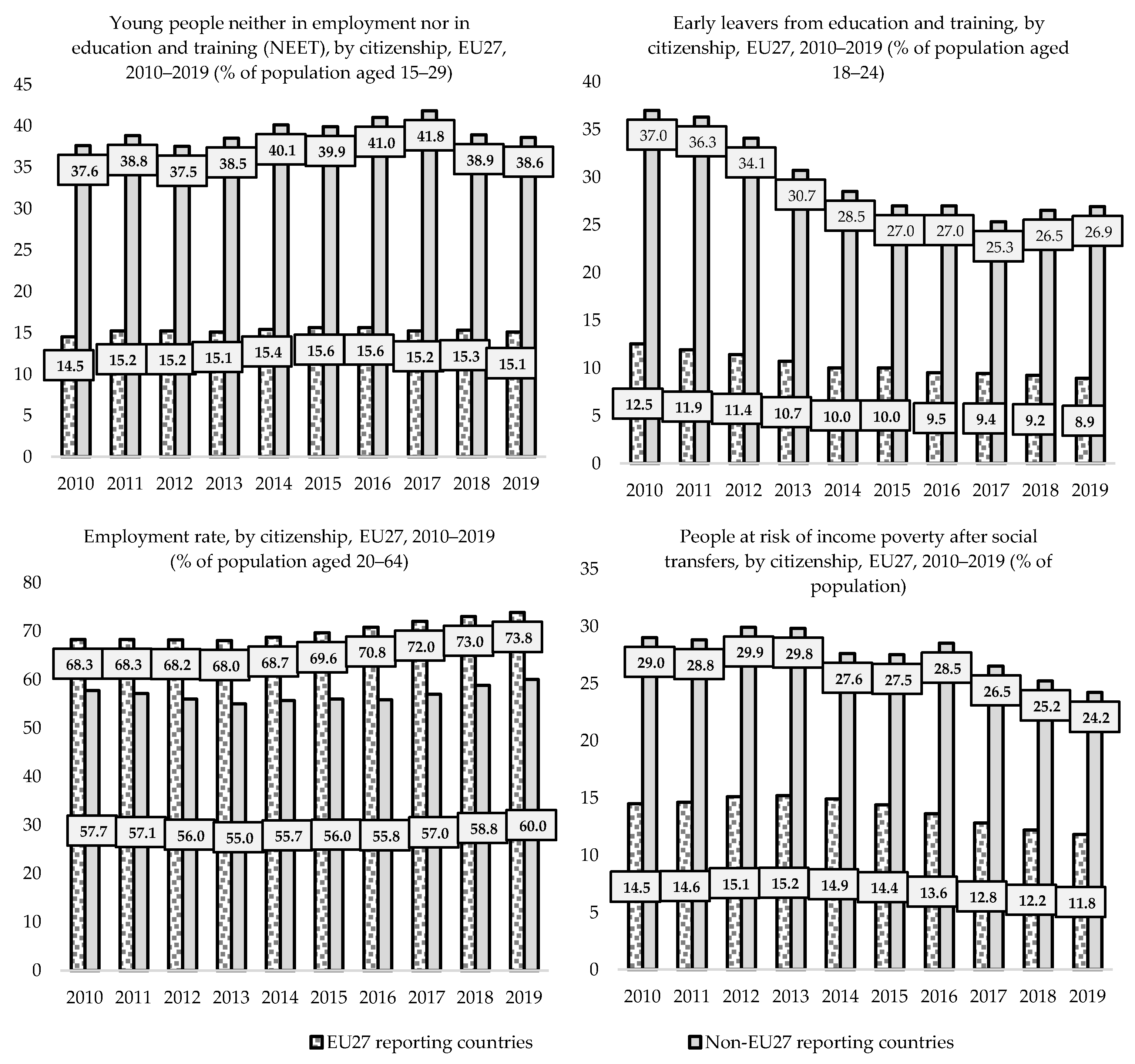
$X_1$—employment rate, only for reporting countries, instead of the citizenship gap (% of population aged 20 to 64),

$X_2$—young people neither in employment nor in education and training (NEET), only for reporting countries, instead of citizenship gap (% of population aged 15 to 29),

$X_3$—early leavers from education and training, only for reporting countries, instead of citizenship gap (% of population aged 18 to 24),

$X_4$—people at risk of income poverty after social transfers, only for reporting countries, instead of citizenship gap (% of population aged 18 years or more),

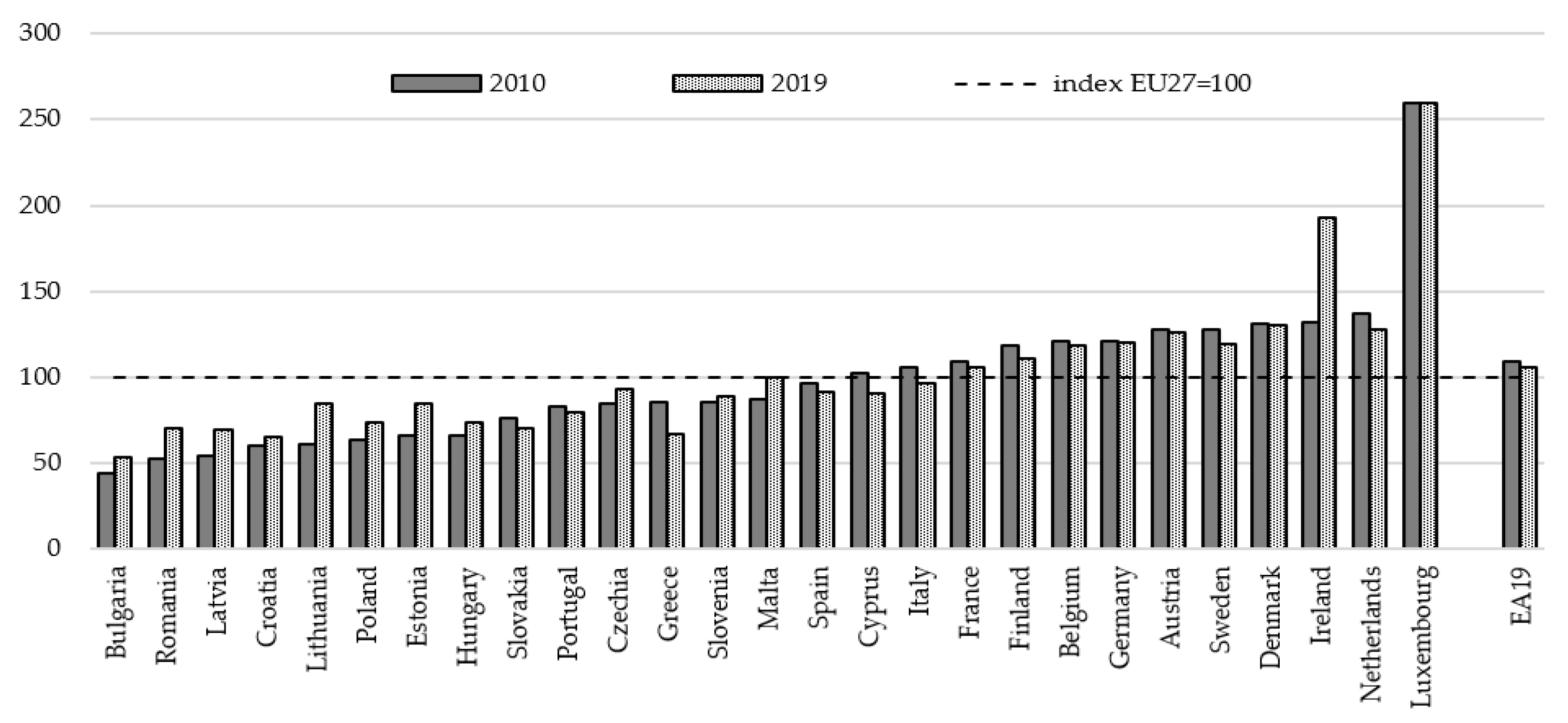
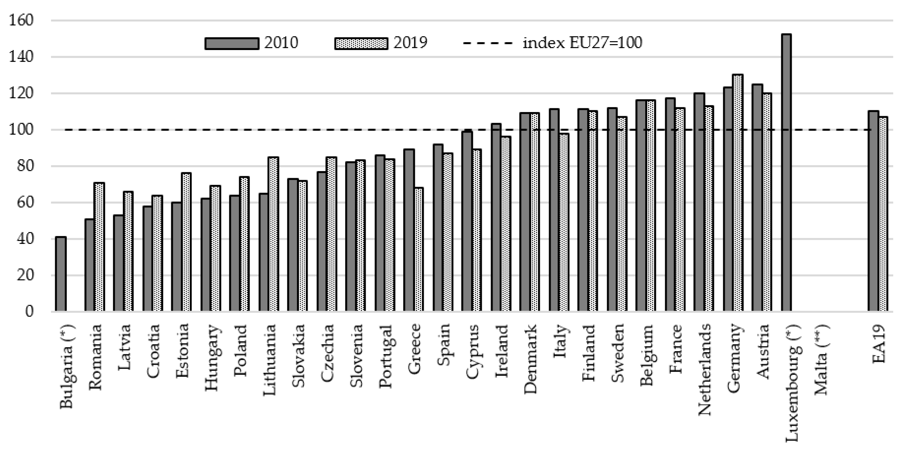
$X_5$—purchasing power adjusted GDP per capita, index EU27 = 100,

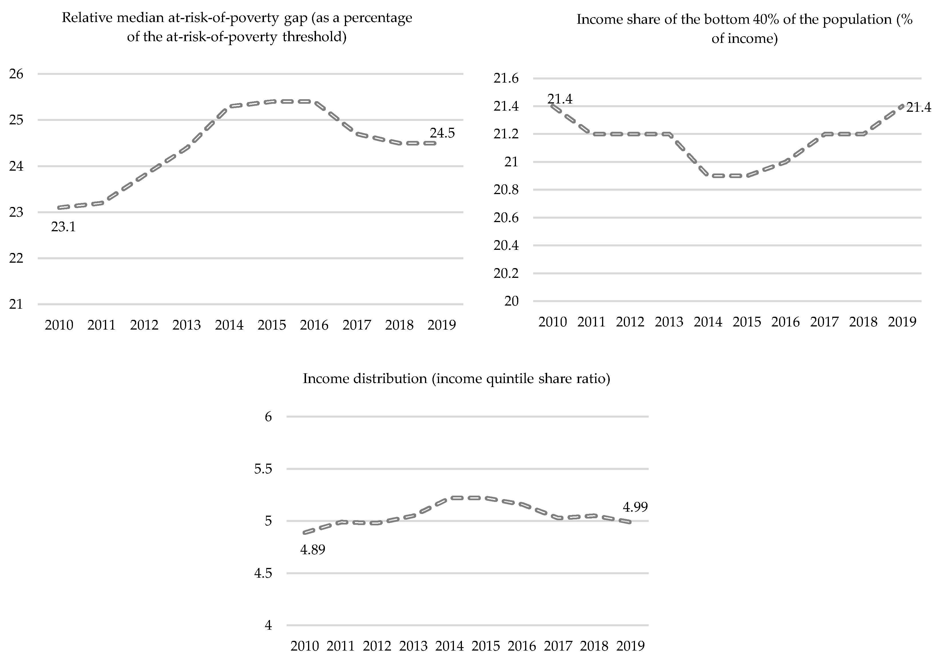
$X_6$—relative median at-risk-of-poverty gap (% distance to poverty threshold),

$X_7$—income distribution (quintile share ratio),

$X_8$—income share of the bottom 40% of the population (% of income).

However, due to potential collinearity between these variables and its consequences for the reduction in the list of variables used in final analyses, additional socioeconomic conditions that may affect the scale of inequalities are included. The extension includes the following control variables for the socioeconomic performance of the EU countries:

$X_9$—Gini coefficient,

$X_{10}$—spending on social protection, % of GDP,

$X_{11}$—proportion of population aged 80 years and more,

$X_{12}$—proportion of population aged 65 years and more,

$X_{13}$—young-age dependency ratio,

$X_{14}$—old-age dependency ratio,

$X_{15}$—total age dependency ratio,

$X_{16}$—purchasing power adjusted GDP per capita growth rate, %.

Selected descriptive statistics for the years 2010 and 2019 are presented in

Table A1. Selected descriptive statistics for chosen set of variables–2010. Source: own work based on Eurostat data.

Variable	Obs.	Average	Median	Min	Max	Range	Variance	St. dev.
$X_1$	27	68.68	68.50	59.90	79.30	19.40	36	5.99
$X_2$	27	13.97	14.00	4.30	23.50	19.20	27	5.20
$X_3$	27	11.16	10.20	4.40	27.80	23.40	40	6.36
$X_4$	27	14.20	13.80	7.40	20.70	13.30	14	3.73
$X_5$	27	98.33	87.00	44.00	260.00	216.00	1842	42.92
$X_6$	27	22.13	21.60	13.80	32.60	18.80	25	4.96
$X_7$	27	4.77	4.49	3.41	7.35	3.94	1	1.07
$X_8$	27	21.70	22.00	17.70	24.90	7.20	5	2.15
$X_9$	27	29.58	29.80	23.80	37.00	13.20	14	3.69
$X_{10}$	27	17.36	17.30	12.10	24.80	12.70	12	3.41
$X_{11}$	27	4.13	4.00	2.70	5.80	3.10	1	0.81
$X_{12}$	27	16.49	16.80	11.20	20.70	9.50	5	2.29
$X_{13}$	27	23.27	22.10	19.20	30.90	11.70	8	2.81
$X_{14}$	27	24.43	25.60	16.50	31.40	14.90	15	3.83
$X_{15}$	27	47.70	47.70	38.80	54.30	15.50	16	4.02
$X_{16}$	27	3.74	4.19	−7.86	10.95	18.81	15	3.93

and

Table A2. Selected descriptive statistics for chosen set of variables–2019. Source: own work based on Eurostat data.

Variable	Obs.	Average	Median	Min	Max	Range	Variance	St. dev.
$X_1$	27	74.98	75.80	61.50	84.50	23.00	31	5.56
$X_2$	27	10.94	10.60	5.20	21.20	16.00	17	4.07
$X_3$	27	8.03	7.30	3.00	15.40	12.40	14	3.72
$X_4$	27	14.89	12.60	9.90	23.60	13.70	17	4.14
$X_5$	27	102.11	91.00	53.00	260.00	207.00	1838	42.87
$X_6$	27	22.40	22.40	14.10	33.00	18.90	29	5.42
$X_7$	27	4.82	4.37	3.34	8.10	4.76	1	1.20
$X_8$	27	21.61	22.30	16.40	25.10	8.70	5	2.29
$X_9$	27	29.67	29.20	22.80	40.80	18.00	16	4.06
$X_{10}$	27	16.17	16.50	8.90	24.00	15.10	17	4.14
$X_{11}$	27	5.12	5.10	3.30	7.20	3.90	1	1.05
$X_{12}$	27	19.33	19.60	14.10	22.90	8.80	5	2.17
$X_{13}$	27	23.91	23.20	20.20	31.40	11.20	7	2.66
$X_{14}$	27	29.77	30.40	20.70	35.80	15.10	15	3.90
$X_{15}$	27	53.69	53.90	43.80	61.40	17.60	18	4.29
$X_{16}$	27	3.83	3.58	0.54	9.60	9.06	4	1.96

in Appendix A. What is more, the set of chosen variables were evaluated while taking into account their informative features. It is important that the set of variables utilized should be characterized by a low degree of correlation (in order to avoid collinearity). The correlation matrices for indicators are presented in

Table A3. Correlation matrix for selected socioeconomic and inequality indicators–2010. Source: own work based on Eurostat data.

	${\mathit{X}}_{\mathbf{1}}$	${\mathit{X}}_{\mathbf{2}}$	${\mathit{X}}_{\mathbf{3}}$	${\mathit{X}}_{\mathbf{4}}$	${\mathit{X}}_{\mathbf{5}}$	${\mathit{X}}_{\mathbf{6}}$	${\mathit{X}}_{\mathbf{7}}$	${\mathit{X}}_{\mathbf{8}}$	${\mathit{X}}_{\mathbf{9}}$	${\mathit{X}}_{\mathbf{10}}$	${\mathit{X}}_{\mathbf{11}}$	${\mathit{X}}_{\mathbf{12}}$	${\mathit{X}}_{\mathbf{13}}$	${\mathit{X}}_{\mathbf{14}}$	${\mathit{X}}_{15}$	${\mathit{X}}_{16}$
$X_1$	1.00
$X_2$	−0.73	1.00
$X_3$	0.13	−0.10	1.00
$X_4$	−0.10	0.08	0.32	1.00
$X_5$	−0.04	0.11	−0.19	−0.63	1.00
$X_6$	−0.07	−0.10	0.14	0.72	−0.53	1.00
$X_7$	−0.19	0.01	0.38	0.86	−0.44	0.82	1.00
$X_8$	0.24	−0.12	−0.42	−0.86	0.39	−0.75	−0.98	1.00
$X_9$	−0.26	0.11	0.42	0.82	−0.39	0.72	0.97	−0.99	1.00
$X_{10}$	0.07	0.07	−0.09	−0.31	0.48	−0.41	−0.36	0.36	−0.37	1.00
$X_{11}$	0.10	0.09	0.23	0.08	0.12	0.05	0.09	−0.09	0.07	0.60	1.00
$X_{12}$	0.02	0.08	0.22	0.39	−0.20	0.33	0.31	−0.29	0.25	0.29	0.83	1.00
$X_{13}$	−0.06	0.13	−0.04	−0.34	0.56	−0.49	−0.24	0.19	−0.18	0.46	−0.06	−0.41	1.00
$X_{14}$	0.02	0.10	0.22	0.37	−0.14	0.28	0.29	−0.28	0.24	0.36	0.87	0.99	−0.30	1.00
$X_{15}$	−0.03	0.19	0.19	0.12	0.26	−0.08	0.11	−0.13	0.11	0.67	0.79	0.66	0.42	0.74	1.00
$X_{16}$	0.21	−0.30	−0.07	−0.08	−0.04	0.04	−0.02	0.05	−0.05	−0.04	−0.21	−0.20	0.03	−0.20	−0.17	1.00

and

Table A4. Correlation matrix for selected socioeconomic and inequality indicators–2019. Source: own work based on Eurostat data.

	${\mathit{X}}_1$	${\mathit{X}}_2$	${\mathit{X}}_3$	${\mathit{X}}_4$	${\mathit{X}}_5$	${\mathit{X}}_6$	${\mathit{X}}_7$	${\mathit{X}}_8$	${\mathit{X}}_9$	${\mathit{X}}_{10}$	${\mathit{X}}_{11}$	${\mathit{X}}_{12}$	${\mathit{X}}_{13}$	${\mathit{X}}_{14}$	${\mathit{X}}_{15}$	${\mathit{X}}_{16}$
$X_1$	1.00
$X_2$	−0.73	1.00
$X_3$	−0.05	0.28	1.00
$X_4$	−0.15	0.39	0.38	1.00
$X_5$	0.10	−0.50	−0.28	−0.48	1.00
$X_6$	−0.44	0.52	0.35	0.62	−0.34	1.00
$X_7$	−0.25	0.45	0.43	0.83	−0.25	0.72	1.00
$X_8$	0.26	−0.41	−0.38	−0.85	0.22	−0.70	−0.98	1.00
$X_9$	−0.23	0.39	0.36	0.77	−0.17	0.61	0.97	−0.98	1.00
$X_{10}$	−0.14	−0.09	−0.20	−0.38	0.18	−0.12	−0.26	0.27	−0.25	1.00
$X_{11}$	−0.29	0.22	0.03	0.38	−0.30	0.33	0.32	−0.35	0.31	0.54	1.00
$X_{12}$	−0.05	0.21	0.18	0.38	−0.56	0.24	0.26	−0.24	0.22	0.41	0.82	1.00
$X_{13}$	0.28	−0.17	−0.28	−0.27	0.35	−0.50	−0.28	0.26	−0.23	0.05	−0.25	−0.33	1.00
$X_{14}$	−0.01	0.20	0.14	0.35	−0.52	0.17	0.23	−0.21	0.19	0.46	0.81	0.99	−0.19	1.00
$X_{15}$	0.16	0.08	−0.05	0.15	−0.26	−0.15	0.04	−0.03	0.03	0.44	0.59	0.70	0.45	0.79	1.00
$X_{16}$	−0.16	0.38	0.32	0.48	−0.35	0.28	0.39	−0.37	0.34	−0.41	−0.12	−0.01	0.06	−0.01	0.03	1.00

in Appendix A. The literature points out that, generally, the correlation between variables should not be strong [41] and that the practice is to use variables with coefficients not exceeding 0.7 [42]. Moreover, in this study there is an assumption that the same set of variables needs to be compared in both years. Therefore, the collinearity in one year affects the decision regarding the reduction of the list of variables in the second year. Such an assumption allows for comparing the same set of features of the economies in both years. The consideration of all requirements and conclusions based on the correlation matrix meant that the final set of variables used in both years is as follows:

$X_1$—employment rate, only for reporting countries, instead of the citizenship gap (% of population aged 20 to 64),

$X_3$—early leavers from education and training, only for reporting countries, instead of citizenship gap (% of population aged 18 to 24),

$X_5$—purchasing power adjusted GDP per capita, index EU27 = 100,

$X_7$—income distribution (quintile share ratio),

$X_{10}$—spending on social protection, % of GDP,

$X_{13}$—young-age dependency ratio,

$X_{14}$—old-age dependency ratio.

Before further analyses, the variables were standardized. Variables $X_1$, $X_3$, $X_5$, and $X_7$ are related to the SDG indicators, but it should be reminded that variables $X_1$ and $X_3$ reflect data only for reporting countries, not a citizenship gap. Moreover, in this study it is assumed that the ranking of countries is built only for data closely related to the SDGs, i.e., on the basis of the application of variables $X_1$, $X_3$, $X_5$, and $X_7$.

In the case of the PCA, after standardizing the set of 16 variables, all 16 were used. The analysis, as a supplementary tool, is applied only to the large dataset available for 2019.

5. Results

The analysis of the EU27 countries with respect to the similarities in socioeconomic backgrounds in the light of the 2030 Agenda is the objective of this session. The outcomes of the used algorithm are presented in the form of dendrograms.

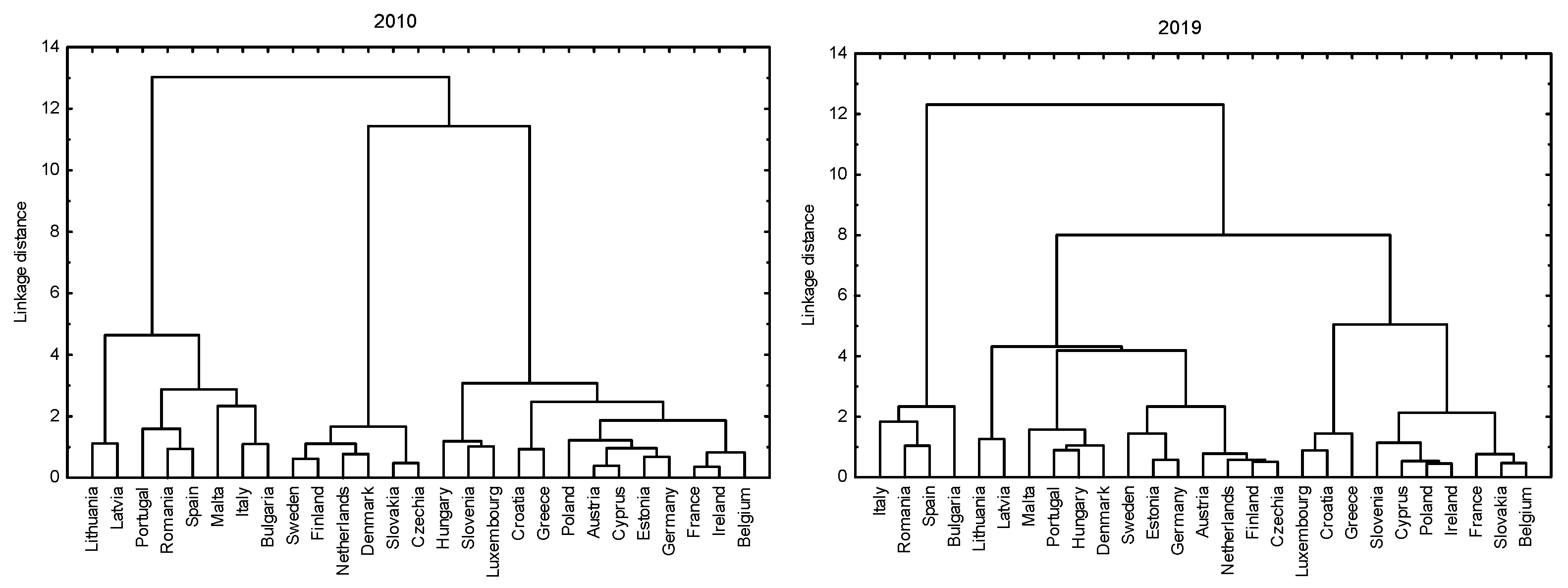
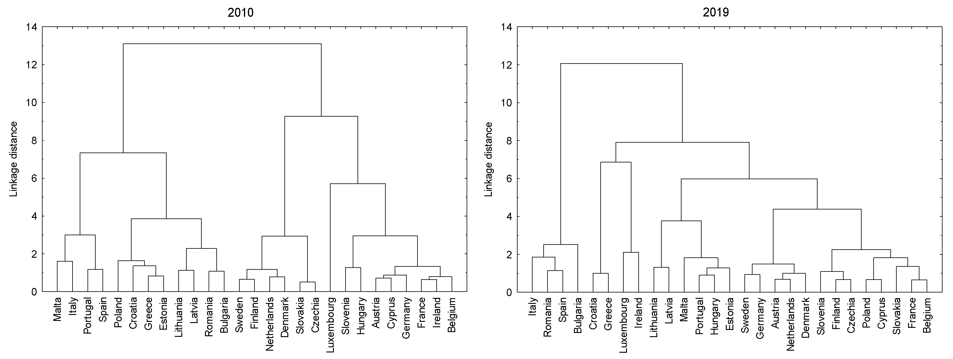
Firstly, cluster analysis of the variables related to SDG10 is carried out in both years in Euclidian space. The dendrograms for the baseline method (i.e., Ward’s method) for the years 2010 and 2019 are presented below (see: Figure 10).

The graphical outcome indicates the division of the countries into two big groups that, under the assumption, differ mostly. In 2010 the first group includes Malta, Italy, Portugal, Spain, Poland, Croatia, Greece, Estonia, Lithuania, Latvia, Romania, and Bulgaria, whereas in 2019 the separate group comprized only Italy, Romania, Spain, and Bulgaria. The conclusion of that observation is that the big dissimilarities of the EU countries in the context of the applied set of variables between 2010 and 2019 are maintained with respect to Italy, Romania, Spain, and Bulgaria in comparison to the rest of the EU. This is due to the fact that between 2010 and 2019 a shift of Malta, Portugal, Poland, Croatia, Greece, Estonia, Lithuania and Latvia is observed with respect to the realization of the four variables analyzed. However, the analysis of the dendrograms and a more detailed analysis of the data emphasize the significant outlier position in 2010 of Luxembourg and in 2019 of Luxembourg and Ireland, which is affected by the $X_5$ variable. Thus, the variable was excluded from the list of indicators, and new dendrograms were generated. The results are presented below.

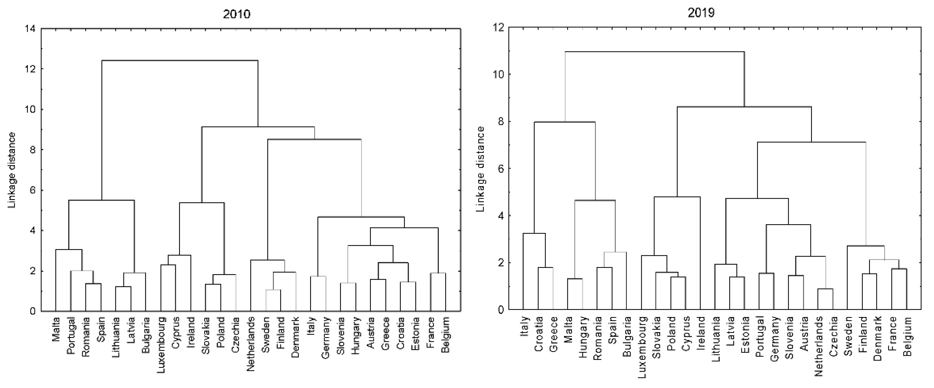
The analysis emphasizes the maintenance of disparities between Italy, Romania, Bulgaria, and Spain and the rest of the European Union countries. Elimination of the $X_5$ variable, which drives the outlier position of a few countries, slightly changed the structure of clusters but allows for further analyses of the dendrograms, especially as Ward’s approach is assumed to be quite sensitive to the outliers (which can impact the results) [32]. The next step is to divide the dendrograms into clusters in order to determine the most similar groups of countries. Figure 11 makes it possible to divide the dendrogram for 2010 into five clusters and the dendrogram for 2019 into six clusters of the most similar countries with respect to the variables analyzed. The structures of the arbitrary extracted clusters are presented in detail in

Table 3. Structure of clusters in 2010 and 2019. Source: own work based on Eurostat data.

	Cluster 1	Cluster 2	Cluster 3	Cluster 4	Cluster 5
2010	Lithuania, Latvia	Portugal, Romania, Spain, Malta, Italy, Bulgaria	Sweden, Finland, the Netherlands, Denmark, Slovakia, Czechia	Hungary, Slovenia, Luxembourg,	Croatia, Greece, Poland, Austria, Cyprus, Estonia, Germany, France, Ireland, Belgium
	(2 countries)	(6 countries)	(6 countries)	(3 countries)	(10 countries)
	Cluster 1	Cluster 2	Cluster 3	Cluster 4	Cluster 5	Cluster 6
2019	Italy, Romania, Spain, Bulgaria	Lithuania, Latvia	Malta, Portugal, Hungary, Denmark	Sweden, Estonia, Germany, Austria, the Netherlands, Finland, Czechia	Luxembourg, Croatia, Greece	Slovenia, Cyprus, Poland, Ireland, France, Slovakia, Belgium
	(4 countries)	(2 countries)	(4 countries)	(7 countries)	(3 countries)	(7 countries)

.

The comparison of the structures of extracted clusters suggests that Latvia and Lithuania in both years create a separate cluster, but in 2019 the two countries were more similar to the rest of the EU than Italy, Romania, Spain, and Bulgaria (which created an outermost linkage with the remaining 23 countries). It may suggest that the inequalities between the group of the aforementioned four countries and the rest of the EU are maintained or even deepened (in the context of the analyzed set of variables). The structure of the clusters points out the similarity of the Netherlands, Czechia, Sweden, and Finland in both years. Countries like Belgium, France, Ireland, Cyprus, and Poland are (together) elements of one cluster in both years. The descriptive statistics for each cluster inform that in 2010, cluster 1 was characterized by the highest intra-cluster average for variable $X_7$—income distribution. Therefore, it denotes that in 2010, Latvia and Lithuania had the highest income inequality (as analyzed from the point of view of the income distribution variable) in comparison to the rest of the clusters. In 2010, the highest intra-cluster average for variable $X_1$ was observed in cluster 3, whereas the highest average for $X_3$ and a quite high average for $X_1$ were observed in cluster 2. In 2019, cluster 1 was created from countries for which the intra-cluster average for $X_3$ and the intra-cluster average for $X_7$ were the highest. In cluster 5 the intra-cluster average for $X_1$ and for $X_3$ were the lowest, whereas in cluster 6 the average was the lowest for $X_7$.

Application of the linear ordering method enables ordering countries with respect to realization of the variables. The division into three groups of countries, analyzed with respect to the computed values for $m_s, m_r$, and $m_i$ is shown in

Table 4. Ranking of countries (higher rank denotes object closer to the ideal pattern). Source: own work based on Eurostat data.

Ranking 2010				Ranking 2019
Rank	${\mathit{m}}_{\mathit{i}}$	Country	Group	Rank	${\mathit{m}}_{\mathit{i}}$	Country	Group
1	0.048	Portugal	I	1	0.005	Bulgaria	I
2	0.128	Spain		2	0.015	Romania
3	0.164	Latvia		3	0.062	Italy
4	0.188	Lithuania		4	0.094	Spain
5	0.264	Romania	II	5	0.164	Greece
6	0.269	Croatia		6	0.299	Malta	II
7	0.319	Greece		7	0.354	Croatia
8	0.343	Hungary		8	0.382	Latvia
9	0.350	Luxembourg		9	0.408	Luxembourg
10	0.362	France		10	0.433	Hungary
11	0.371	Malta		11	0.453	Portugal
12	0.389	Ireland		12	0.462	Lithuania
13	0.404	Bulgaria		13	0.508	France
14	0.439	Estonia		14	0.512	Belgium
15	0.465	Italy		15	0.530	Slovakia
16	0.471	Belgium		16	0.558	Estonia
17	0.474	Austria		17	0.558	Poland
18	0.512	Cyprus		18	0.602	Denmark
19	0.520	Slovenia		19	0.630	Cyprus
20	0.561	Germany		20	0.639	Ireland
21	0.589	Poland		21	0.655	Germany
22	0.704	Denmark	III	22	0.687	Finland
23	0.774	the Netherlands		23	0.714	Slovenia
24	0.793	Slovakia		24	0.733	Austria	III
25	0.826	Finland		25	0.736	the Netherlands
26	0.877	Czechia		26	0.760	Czechia
27	0.902	Sweden		27	0.818	Sweden
$m_s$= 0.234; $m_r$ = 0.695				$m_s$= 0.263; $m_r$ = 0.732

.

Computing values $m_s$, $m_r$, and $m_i$ separately for each year allows dividing the countries with respect to realization of the analyzed set of variables. As presented, the group with weak realization of the variables in comparison to the pattern in both years consists of four countries, but only Spain is attributed by the approach to the I group in both years. The numbers of countries in the group of the best performers (i.e., group III) in both years differ, consisting of six countries in 2010 and four countries in 2019, but in both years the group includes the Netherlands, Czechia, and Sweden. In 2010 the disparity in development measure$m_i$ between the “worst” country and the “best” country is around 0.854, whereas in 2019 it is around 0.768. This implies a reduction in disparity between two extreme countries. Sweden in 2010 was computed as being a country closer to the ideal pattern (due to the value being closer to 1 in 2010 than in 2019). Sweden and Czechia are attributed by the linear ordering method as being the best performers, but the disparity between these countries (as measured via $m_i$) was lower in 2010 (the distance is around 0.025 in 2010 and 0.058 in 2019). On the other hand, the difference in $m_i$ between the “worst” and the second-worst countries was higher in 2010 than in 2019. In 2010, Spain held the second-to-last place and in 2019 the fourth, but its position in 2019 was closer to the anti-pattern due to the lower value of $m_i$. Moreover, in 2010 the difference between two distinguished best performers was lower than the difference between two worst performers—the opposite situation was in 2019.

Finally, the outcome generated on the basis of Ward’s method and the squared Euclidian distance for a set of all variables is presented in Figure 12. Due to the impact of the $X_5$ variable on the outlier positions, the variable, as previously, was excluded from the dataset.

The analysis of the dendrograms affects, as previously, the decision to distinguish the clusters, whose structures are presented in

Table 5. Structure of clusters in 2010 and 2019. Source: own work based on Eurostat data.

	Cluster 1	Cluster 2	Cluster 3	Cluster 4	Cluster 5	Cluster 6
2010	Malta, Portugal, Romania, Spain	Lithuania, Latvia, Bulgaria	Luxembourg, Cyprus, Ireland	Slovakia, Poland, Czechia	the Netherlands, Sweden, Finland, Denmark	Italy, Germany, Slovenia, Hungary, Austria, Greece, Croatia, Estonia, France, Belgium
	(4 countries)	(3 countries)	(3 countries)	(3 countries)	(4 countries)	(10 countries)
	Cluster 1	Cluster 2	Cluster 3	Cluster 4	Cluster 5
2019	Italy, Croatia, Greece	Malta, Hungary, Romania, Spain, Bulgaria	Luxemburg, Slovakia, Poland, Cyprus, Ireland	Lithuania, Latvia, Estonia, Portugal, Germany, Slovenia, Austria, the Netherlands, Czechia	Sweden, Finland, Denmark, France, Belgium
	(3 countries)	(5 countries)	(5 countries)	(9 countries)	(5 countries)

.

The comparison of the structure of clusters indicates that in both years, Romania, Spain, Malta, and Bulgaria are included in the first “big” cluster, exhibiting persistent derogation from the rest of the EU countries. Furthermore, in both years, Malta, Romania, and Spain are structured in one cluster. A similar conclusion can be formulated in the cases of Sweden, Finland, and Denmark—these countries are elements of one cluster in both years. In 2010, cluster 1 was characterized by countries whose intra-cluster average of variable $X_3$ was the highest. The highest intra-cluster average for cluster 2 concerned variable $X_7$ (highest income inequality), whereas the lowest was observed for $X_{13}$ and $X_{10}$. Cluster 3 had the highest average for $X_{13}$ and the lowest for $X_1$ and $X_{14}$, whereas the highest intra-cluster average for $X_{14}$ was seen in cluster 6. The lowest intra-cluster average for variable $X_7$ was observed in cluster 5, for which the averages for $X_{10}$ and $X_1$ were the highest among all six extracted clusters. In the case of 2019, cluster 1 was characterized by countries with the lowest intra-cluster average for $X_1$ and $X_{13}$ and the highest average for $X_{14}$. Cluster 2 was characterized by a high intra-cluster average for $X_3$ and $X_7$ and the lowest average for $X_{10}$. The highest intra-cluster average for $X_{10}$ and $X_{13}$ and the lowest average for $X_7$ were observed in the case of cluster 5 (grouping Sweden, Finland, Denmark, France, and Belgium).

The PCA method makes it possible to reduce the dataset dimensionality. As mentioned previously, the initial set of potentially correlated variables is used. The presented analysis is based only on 2019. This procedure makes it possible to obtain the principal components and eigenvalues, presented in

Table 6. PCA results for 2019. Source: own work based on Eurostat data.

Component	Eigenvalue	Variance (%)	Cumulative Eigenvalue	Cumulative Variance (%)
1	6.030032	37.687703	6.030032	37.687703
2	3.507873	21.924207	9.537905	59.611909
3	1.688226	10.551411	11.226131	70.163320
4	1.402679	8.766742	12.628810	78.930062
5	1.291465	8.071654	13.920275	87.001716
6	0.734132	4.588323	14.654406	91.590039
7	0.445659	2.785370	15.100065	94.375408
8	0.329912	2.061950	15.429977	96.437359
9	0.244694	1.529339	15.674672	97.966697
10	0.156645	0.979028	15.831316	98.945726
11	0.090906	0.568160	15.922222	99.513885
12	0.059793	0.373707	15.982015	99.887592
13	0.012193	0.076209	15.994208	99.963801
14	0.005417	0.033857	15.999625	99.997658
15	0.000337	0.002108	15.999963	99.999766
16	0.000037	0.000234	16.000000	100.000000

below.

The first component identifies around 38% of the total variance, whereas the sum of the first and second components identifies about 60% of the total information included in the initial variables. However, an important step in this method is to decide on the number of components to be potentially taken into account in any further analysis. As mentioned, in this study, Kaiser’s [40] approach is adopted, and as a result, the first five components are taken for further considerations. The amount of the variance retained by the first five components is around 87%. As a result, in the further analysis, the number of components was reduced to the first five components by losing only around 13% of the information included in the initial set of variables. The transformation of the set of variables into a set of components makes it possible to illustrate multivariate data.

Table 7. Coefficients of the first five components. Source: own work based on Eurostat data.

Variable	Component 1	Component 2	Component 3	Component 4	Component 5
$X_1$	0.159532	0.058265	−0.551728	−0.093570	−0.428331
$X_2$	−0.254184	−0.060446	0.272186	0.353364	0.387998
$X_3$	−0.195329	−0.113733	−0.074660	0.171207	−0.264540
$X_4$	−0.352664	−0.090292	−0.217633	−0.030831	−0.053005
$X_5$	0.231227	−0.104764	0.028492	−0.556256	0.214493
$X_6$	−0.313102	−0.128932	0.234069	−0.084685	−0.048320
$X_7$	−0.358875	−0.152914	−0.113491	−0.256453	0.050010
$X_8$	0.353376	0.157097	0.117189	0.292928	−0.064538
$X_9$	−0.334776	−0.153249	−0.135695	−0.321691	0.082098
$X_{10}$	0.049090	0.398008	0.267575	−0.228623	0.162521
$X_{11}$	−0.233394	0.372125	0.130506	−0.191768	0.038250
$X_{12}$	−0.237145	0.408742	−0.019018	0.070096	−0.185272
$X_{13}$	0.172720	0.045826	−0.437209	−0.003003	0.579784
$X_{14}$	−0.218874	0.434790	−0.078628	0.064405	−0.096678
$X_{15}$	−0.092197	0.424254	−0.342340	0.056485	0.272449
$X_{16}$	−0.175547	−0.193974	−0.253821	0.403931	0.222540

shows the coefficients of the components.

The additional analyses of the PCA results indicate that the first component is mainly affected by the information loaded by variable$X_7$, the second—by variable$X_{14}$, the third by$X_1$, the fourth by$X_5,$ and the fifth by$X_{13}$. The results are interesting because they confirm the final set of uncorrelated data included in the multivariate methods (see the description of the result for the cluster analysis and the linear ordering method).

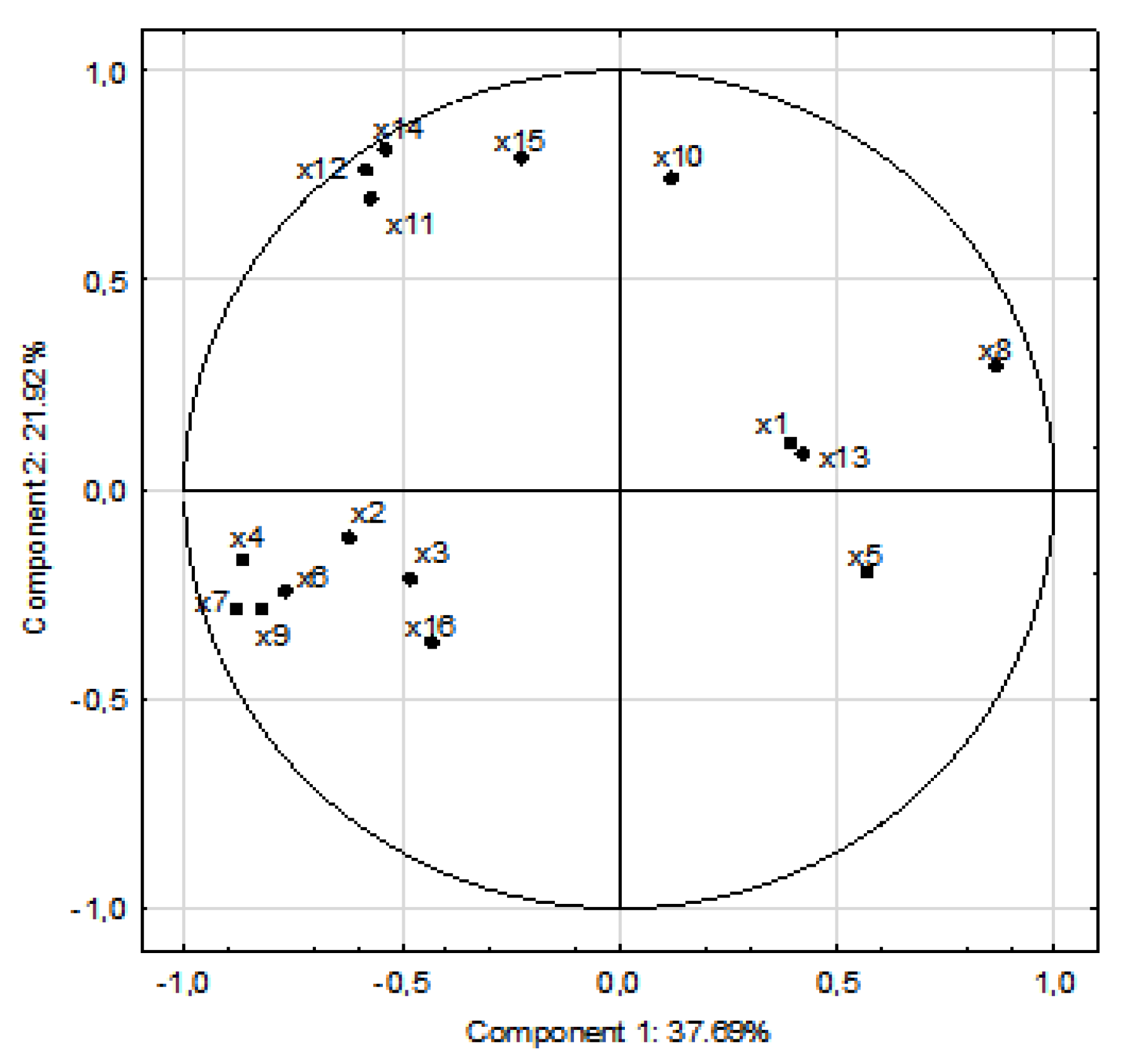
Figure 13 below shows the indicators in the PCA on the correlation circle according to the first two principal components.

The circle indicates the outlier position of the $X_5$ variable—purchasing power adjusted GDP per capita, index EU27 = 100, which was also recognized in previous analyses, based on the linear ordering method and cluster analysis. Figure 13 shows a group of indicators. For example, one of the visible groups consists of the variables $X_{11}$—the proportion of the population aged 80 years and more, $X_{12}$—the proportion of population aged 65 years and more, $X_{14}$—the old-age dependency ratio, and $X_{15}$—the total age dependency ratio, i.e., variables mainly related to the “old” population. It is also possible to include variable $X_{10}$—spending on social protection as a% of GDP, which is correlates more with the “older” than “younger” structure of the population. The second visible group concerns indicators related to variable $X_4$—people at risk of income poverty after social transfers, (indicator only for reporting countries, instead of citizenship gap, as used previously (% of population aged 18 years or more),$X_6$—the relative median at-risk-of-poverty gap (% distance to poverty threshold), $X_7$—income distribution (quintile share ratio), and $X_9$—the Gini coefficient. When comparing countries, the dimension that involves the two first components confirms the disparities between EU countries. The PCA method applied for the 2019 dataset investigates disparities between countries, emphasizing the outlier position of the euro area peripheral countries (Italy, Greece, and Portugal) and also the outlier position of Romania and Bulgaria. The results also allow us to conclude about the division of the analyzed countries based on whether they are “new” or “old” European Union countries; however, the exceptions of Ireland and Luxembourg (as with previous analyses using the linear ordering method and cluster analysis) is also shown.

6. Discussion

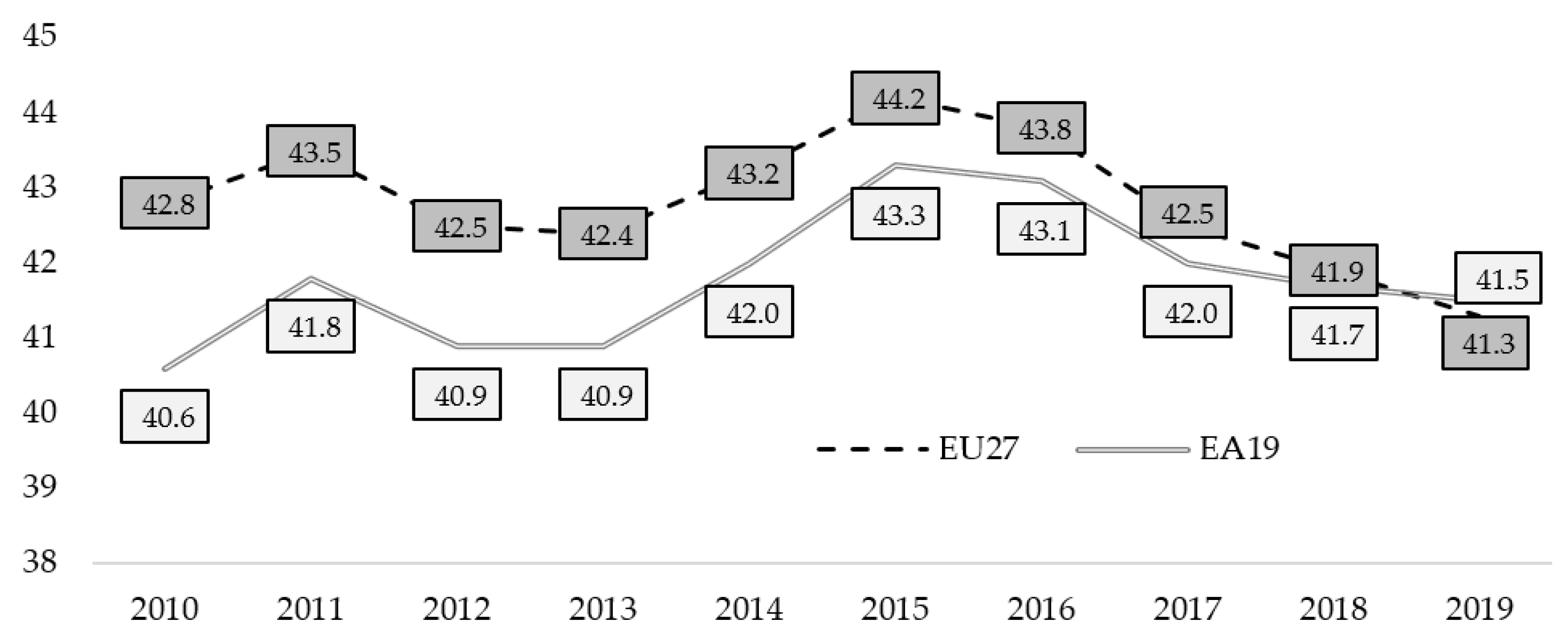
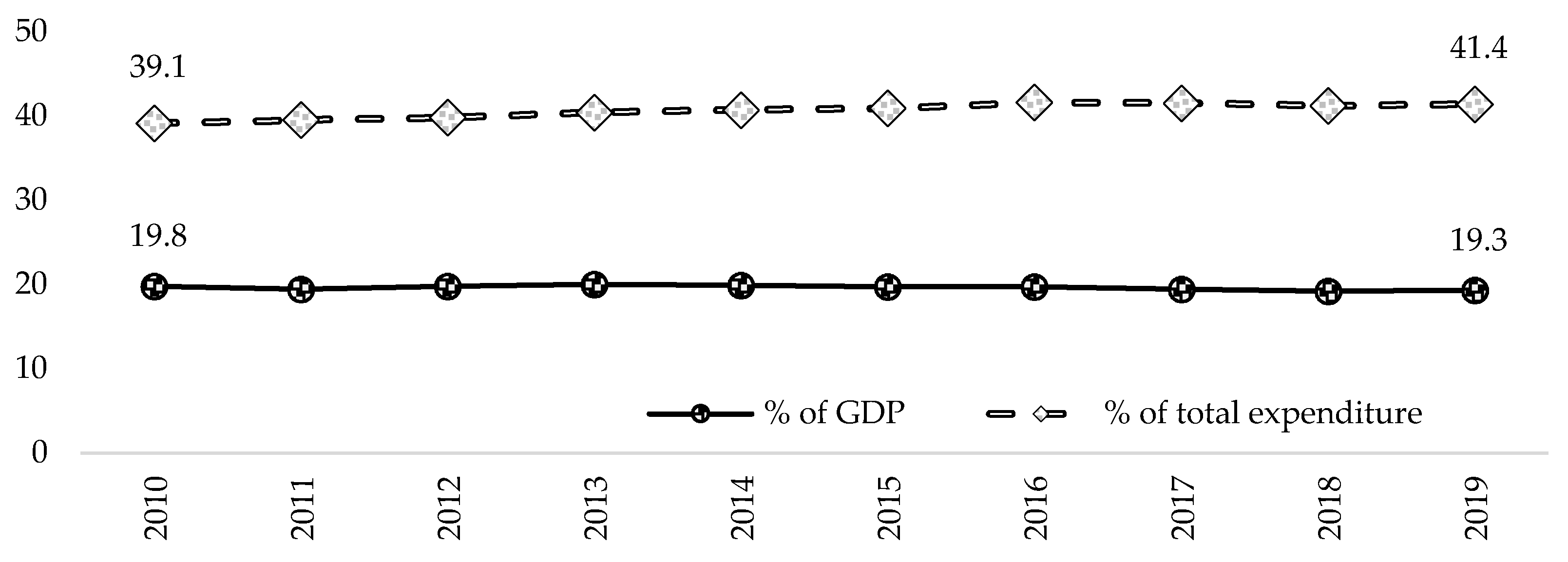
The analysis of the dynamics of the SDG10 indicators at the aggregated EU27 level emphasizes that between 2010 and 2019 the European Union was unable to reduce inequalities in all aspects analyzed. Although in the medium term, essential progress has been made with respect to the indicator measuring the reduction in disparities in household disposable income per capita, the indicator of the citizenship gap for early leavers from education and learning, or the indicator of the citizenship gap for the NEET rate, within-country inequalities persist. The analysis of three within-country inequalities informs that from 2010–2015 the disparities in the EU27 as a whole increased but there was a reduction observed from 2016–2019, but in 2019 the level of the three SDG10 indicators analyzed was generally higher than in 2010. In 2019, in comparison to 2010, the within-country inequalities slightly increased on average. The analysis of SDG10 indicators suggests the maintenance or even deepening of poverty in the EU. Despite this, some countries were able to reduce the inequalities; however, some of them worsened their position. The extended analysis provided by means of the use of selected socioeconomic indicators shows that the EU27 as a whole increased the share of social spending as a percentage of total spending over 2010–2019, but the size of the increase differs regardless of the group of countries and their structural characteristics.

The applied multivariate analysis, which is cluster analysis, supported by the use of the linear ordering method, provides important insights. The assessment of the (dis)similarities of the countries with respect to the chosen set of socioeconomic variables indicates that Spain, Romania, and Bulgaria maintain their position and are included in the most different group of countries in comparison to the rest of the EU. Such distinctiveness remains regardless of the analyzed year or the set of inputted variables. Contrary to these countries, there is a group of countries that are characterized by a low level of inequalities. For example, a relatively low poverty gap was observed in Czechia, the Netherlands, and Finland. Moreover, the use of an ordering method supports the insights obtained in cluster analysis. The ordering method emphasizes the high position of Sweden and Czechia as countries with good performance of individual country-level indicators, while cluster analysis allows inputting them into one cluster.

The analyses presented in this study contribute to the conclusion that, despite cohesion policy, inequalities, especially within-country inequalities, remain in the EU and there are persistent disparities. Furthermore, the presented values for the Gini coefficient illustrate that between 2010 and 2019 the income inequalities measured by this indicator decreased only in the case of 15 countries, but the size of the largest reduction (by 3.1 units in Slovakia) was nearly two times lower than the largest size of its increase (by 7.6 units in Bulgaria).

It is worth emphasizing that the cluster analysis based on the extended list of indicators highlights an important conclusion. The cluster for which the intra-cluster average for the income distribution variable was the lowest among the extracted countries, at the same time, had the highest intra-cluster average for spending on social protection, regardless of the year analyzed. The reverse also occurred—the cluster for which the average for income distribution was the highest, at the same time, was the cluster for which the average for social protection spending as a share of GDP was the lowest. This insight emphasizes the role of social policy in mitigating and reducing inequalities, especially within-country inequalities. The aforementioned relationship is also visible in correlation matrices for all datasets (see Table A3 and Table A4 in Appendix A). For all of the EU27 countries, Pearson’s correlation coefficient between variables $X_7$ and $X_{10}$ is negative. In 2010 it is computed to be equal to −0.36 and in 2019 its value is −0.26. The correlation matrices also confirm the positive relationship between the old-age dependency ratio and social protection spending and between the young-age dependency ratio and social protection spending. The importance of the Agenda and SDG10 has increased in the context of the COVID-19 pandemic. This is because the pandemic has affected social and economic dimensions of countries all over the world.

The literature review did not provide similar studies that analyzed the performance of SDG10. However, in the context of implementing the 2030 Agenda, the existing literature leads to the same conclusion as expressed in this paper about the need for political and government support to successfully achieve the goals of the Agenda. This has recently been emphasized in the context of the crisis caused by the COVID-19 external shock. The pandemic has maintained or even deepened inequalities, mainly income disparities, both among and within countries, and made a few groups of people more vulnerable to the economic consequences of the crisis.

The results of the study are valuable and may support further research and further debates surrounding the role of social protection policies and sources of financial activities in order to progressively achieve greater equality.

7. Conclusions

This paper aims to analyze the progress of the EU27 with regard to SDG10 (which is assigned to reduce inequalities between and within countries). In order to achieve that goal, two studies are proposed. The first study is based on an analysis of the dynamics of SDG indicators for the EU27, while the second - on multivariate analysis that makes it possible to classify European Union countries from the point of view of their (dis)similarities with respect to a wider set of socioeconomic indicators. As a result, the multivariate analyses (i.e., cluster analysis and linear ordering method) are based on a set of variables including selected SDG10 indicators and selected socioeconomic variables that may affect the reduction of inequalities. The timeframe of the analyses, due to data availability, spans 2010 to 2019. All considered SDG indicators and analyzed socioeconomic variables derive from Eurostat.

The dynamics of the SDG10 indicators for the EU27 emphasize that between 2010 and 2019 the inequalities within countries slightly increased. The analysis implies that over the medium term (i.e., over the period 2010–2019) the EU27 was able to make progress in reducing inequalities among countries, but the income inequalities within countries persist or have even deepened. The insights from multivariate statistical methods emphasize the disparities between a group of countries (including Spain, Bulgaria, and Romania) and the rest of the EU countries in both analyzed years (i.e., in 2010 and 2019), regardless of the set of variables applied in analyses. This outcome seems to be robust, considering the methodology utilized. Furthermore, cluster analysis, as well as the PCA, points out the division of the EU27 into Western and Eastern countries as well as “old” and “new” EU member states. It implies that although the EU has an advanced cohesion policy, income inequalities and social exclusion persist in the EU. Another important insight from cluster analysis concerns the role of expenditure on social protection. As obtained, a cluster for which the intra-cluster average for income distribution is the lowest among separated clusters in the analyzed year, at the same time, is a cluster for which the intra-cluster average for social protection expenditure is the highest. The reverse is also confirmed. This observation emphasizes the potential role of social spending in mitigating inequalities. Moreover, the role of demography, especially aging, is emphasized in this study as being a factor affecting inequalities due to the advanced process of aging in Europe.

A few limitations should be emphasized. For example, the study is restricted by data availability. The lack of data, especially on SDG10 indicators addressing the citizenship gap at a country-specific level, determines a set of variables included in analyses and reduces their important impact on outcomes. As a result, the wider among- and within-country comparisons are obstructed. Moreover, due to collinearity, a large set of SDG10 indicators was excluded from multivariate analyses. Taking into account the results, there is a need for public policies to strengthen actions to achieve SDG10. The recognized inequalities harm sustainable development and impact the quality of life, mainly of the most vulnerable groups, including the old, the disabled, the unemployed, or migrants. The policies should encourage equality and eliminate disparities related to income, education level, gender, age, country of origin, and many other aspects.

The approaches that were used in the paper identified the group of countries that differ in the EU, emphasizing the division into “old” and “new” EU Member States. It is a crucial observation and a challenge for the EU as a whole because the inequalities were maintained over the 2010–2019 period. It shows that the cohesion policy is not sufficient and requires additional activities to help eliminate the disparities. Taking into account the analyzed data, goals, indicators, time sample, and results of the multivariate analyses, a few potential directions of the development of those policies can be outlined. These directions may take into account aspects that involve demographic changes, environmental changes, and globalization. An important point is related to the challenges created by the COVID-19 pandemic and its economic, social, and health consequences. The crisis revealed the need for governments to work to overcome the socioeconomic effects of the downturn, especially in terms of active and adequate social policies. Moreover, as emphasized, one factor that impacts the increase in the inequalities is the aging of society, which affects all EU countries. It seems that an appropriate social policy (mainly social security system, pension system, health care, long-term care) could effectively support the cohesion policy and, as a consequence, contribute to the more persistent reduction of inequalities. That policy could be conducted at the national level while also considering the common European social policy aspect. As presented in the study, the external shock, in the form of the pandemic, hindered the progress in reducing inequalities among and within EU countries, not only in terms of SDG10 but also the 2030 Agenda as a whole, i.e., through the scale of the interactions and the impact of SDG10 on the other SDGs.

As emphasized, the results of this study may contribute to debates surrounding the actions taken by policymakers to strengthen the progress towards SDG10. Mainly, there is a need for effective country-specific policies that could affect the areas responsible for building resilient societies and achieving sustainable development and the social inclusion of all. These debates should also focus on financing such policies and searching for more sustainable and efficient sources of funds. The study may support and stimulate further research because of the growing importance of the 2030 Agenda in reducing inequalities and the growing threat of escalation of poverty and income inequalities of many vulnerable groups of people. The results obtained in this study are valuable, especially in the context of the role of the 2030 Agenda in reducing inequalities caused by the COVID-19 pandemic.