Assessment Environmental Sustainability and Gender Equality through Crops Livestock Investment Worldwide

Simple Summary

Investing in live-crops technology reduces gender gap employment in rural areas while increasing temperature change.

Abstract

Resilient crop-livestock production systems become crucial to face environmental challenges such as climate mitigation. Progress in the SDG 2.4.1 indicator (proportion of agricultural area under productive and sustainable agriculture) requires robustness, adaptability, and transformation. Most literature considers gender equality and crops livestock investment as drivers to environmental sustainability. In Cosculluela-Martínez (2020), the productivity and the employing capacity of the investment in agricultural capital stock has been analyzed. However, nobody has examined the long and short-run effects on climate change and the gender gap of investing in the crop-livestock production system’s assets. In this paper, the investment’s empowerment is assessed by estimating the impact of an investment in capital stock on climate, gender gap drop-down, and production through a Vector Error Correction Model. To reduce the gender gap in the agricultural sector in 8 of the 11 countries. Policy and implications of different weights in the distribution of the investment of European Funds are discussed.

1. Introduction

The agricultural sector also has significant negative impacts on climate change, sometimes something hidden and underestimated. According to Food and Agriculture Organization of the United Nations (FAO), agriculture contributes around 15 to 20 percent of the world’s greenhouse gas emissions (GHG). Based on data from the meta-analysis conducted by Poore and Nemecek (2018), food is responsible for approximately 26% of global GHG emissions (while Agriculture, Forestry and Land use directly accounts for 18.4% of GHG emissions, the food system accounts for around one-quarter of GHG. Crop production accounts for 27% of food emissions and Livestock & Fisheries account for 31%).

On the other hand, following FAO (2020) [1], Gross Fixed Capital Formation in agriculture increased by about 29 percent between 2010 and 2017, from USD 477 to USD 617 billion in constant 2010 USD. Agricultural investment rates grow faster in high-medium income countries where the agricultural sector is more capital-intense than in low-income countries. The agricultural investment ratio improved in the 2010–2017 period, increasing by about 16 percent, following a growing trend. In Northen America and Europe is registered a more sustained growth.

Gender equality (SDG 5) is an overall worry in most societies and socio-economic activities becoming pivotal to achieve productivity increases, hunger reduction, and, specifically, the Sustainable Development Goal 2 (SDG 2) (end hunger, achieve food security and improved nutrition and promote sustainable agriculture). Hence, achieving agricultural sustainability and climate adaptation depends on gender equality (Bryan, 2019; FAO, 2018; Ignaciuk and Chi Tun, 2019) [2,3,4].

Considering the above data and information, a crucial concern is how to double agricultural production and promote social justice (gender equality) without harming the environment. At the same time, agriculture must be more productive, efficient, sustainable, and socially fair and inclusive.

To achieve these goals, crop-livestock systems require huge investment volumes, innovative business models, and intelligent technologies to foster productivity and efficiency and gender equality to be inclusive. Gender equality is a pivotal condition for transforming food systems, but also food systems can be an opportunity for women’s empowerment.

To properly discuss the results in a sustainability framework, we introduce the transformative approach to resilience. Resilient agricultural systems are a key determinant of sustainability. However, not all resilience approaches fit sustainability understood as a future-oriented science, policy, and practice. Socio-ecological systems, as the crop-livestock, need to be managed by a transformative approach, overcoming features and goals as returning to the previous state after a shock or crisis, resistance, to be robust, shock-absorbing, and others of similar meaning. In this context, agricultural transformation faces the challenge of maintaining the level of agricultural production necessary to feed the world and apply practices focused on sustainable production. As conceptualized in Singh, Hudson, and Donkor (2010, p. 6) [5] (following Singh, Hudson, and Donkor (2010) [5], resilience considers production while acknowledging gradual degradation of the system (e.g., soil erosion, impoverishment of biodiversity, nutrient depletion) and unexpected shocks (e.g., pest outbreaks)), agriculture sustainability comprises “practices that meet current and future societal needs for food and fiber, ecosystem services, and healthy lives while appropriately accounting for all costs and benefits”. In short, crop-livestock and other agricultural systems require transformation.

A recent work of Cosculluela-Martínez (2020) [6] compares the effect produced by a permanent unitary shock in Sustainable Knowledge capital stock for the Primary Sector on the Spanish employment and GDP growth with the effect produced by the other fourteen capital stock types. However, to the best of our knowledge, no research has examined the long and short-run effects on climate change and the gender gap of investing in the crop-livestock production system’s assets.

In this paper, with variables offered by the FAO organization, the effects of a shock in agricultural, forestry and fishing net capital stock (NCS) on employment-to-population ratios, climate change and value added is computed for a time-span of 15 periods.

Thus, we hypothesize that:

Hypothesis 1.

Some countries have much higher gender gap drop-down due to the investment in NCS (Agriculture, Forestry and Fishing).

Hypothesis 2.

Long run effects on climate change are present in all the countries when increasing NCS for the Agriculture, Forestry and Fishing.

Hypothesis 3.

Which countries have the higher climate reverse effect investing a one percentage point in NCS (Agriculture, Forestry and Fishing).

To check these hypotheses, we estimated a Vector Error Correction Model (VECM). This technique allows mutual causality between the variables and different differed effects between them. It is adequate because its simple orthogonalized form allows considering the effect simultaneously, instantaneously and differed, without constraints on prior grounds; the data determines through the significance of the correlation the possible instant effects. This methodology has been widely used for the estimation of effects of a shock in economic variables since Aschauer’ seminal works [7,8,9], using different types of data, at different geographic levels and countries, and considering or not cointegration or the properties of time series.

The contribution of this paper lies on the evaluation of the effects of each country separately. Thus, for each country with enough data span the coefficients of one VECM is estimated in its conveniently orthogonalized reduced form. This individual estimation allows the estimation of singular effects for each country in the different periods without imposing that the behavior of the countries are the same.

The rest of the paper is organized as follows: Section 2 shows the literature review. In Section 3, the methodology applied, the series used and their statistical properties, and the empirical estimation. In Section 4, we discuss the Impulse Response Functions (IRFs) of male and female employment, output, and climate change. Finally, Section 5 points out the concluding remarks and possible limitations.

2. Literature Review

Target 2.4 of the Sustainable Development Goals tries to ensure by 2030 sustainable food production systems and implement resilient agricultural practices that increase productivity and production, that help maintain ecosystems, and strengthen the capacity for adaptation to climate change. In addition, to achieving this target (and others), FAO’s Sustainable Food and Agriculture (SFA) approach is articulated in five principles (1) Increase productivity, employment, and value addition in food systems; (2) Protect and enhance natural resources; (3) Improve livelihoods and foster inclusive economic growth; (4) Enhance the resilience of people, communities and ecosystems, and (5) Adapt governance to new challenges.

However, from the first years of this century, there is a feeling that environmental conditions change quickly, abruptly, and unpredictably requiring transformative approaches, policies, and practice. These approaches include restructuring, path-shifting, innovation, multiscale, and systemwide (Fedele et al., 2016) [10]. Besides, as Revi et al. (2014) [11] commented, transformative adaptation opens policy choices. Between them, environmental innovation positively impacts firms´ productivity (Aldieri, Makkonen, and Vinci, 2020) [12] and applying ecological footprint models to achieve an optimal allocation of resources (Wang, Huang, Zhou, Deng, and Fang, 2020) [13]. In this article, we analyze gender equality and Fixed Capital Formation as transformative policy options.

Fixed Capital Formation is a driver to agricultural productivity and production growth, development, poverty, and hunger reduction, being crucial at the farm level. Vander Donkt and Chan (2019) [14] presented new estimates of the agricultural investment ratio, which are then used to construct a wider capital stock database in the agriculture sector worldwide by applying a variant of the Perpetual Inventory Method (PIM). Later, Vander Donkt, Chan, and Silvestrini (2020) [15] developed a new analytic database on aggregate physical investment flows and capital stock in agriculture, forestry, and fishing (1995–2017) to estimate the Perpetual Inventory Method.

On the other hand, achieving agricultural sustainability depends on gender equality (Bryan, 2019; FAO, 2018; Ignaciuk and Chi Tun, 2019) [2,3,4], and several obstacles and constraints undermine this progress: in highly unequal countries, the majority of the farming population, particularly women, lacks the economic resources and capacity to invest in appropriate agricultural technologies, as well as the knowledge to implement improved agricultural practices. According to Ignaciuk and Chi Tun (2019) [4] and FAO (2018) [3], women also have difficulty accessing land ownership, extension services, and finance (agricultural credit, for instance). Progress in removing these barriers and obstacles and women empowerment is necessary and monitored by the Women’s Empowerment in Agricultural Index.

Climate change also impacts the global food system. For example, it affects crop yields and nutrition outcomes by lowering the nutritional value of crops and disrupting activities along food value chains (Bryan, 2019) [2]. However, men and women have different adaptation capacities due to an unequal availability of resources: overall, women have less information about climate change, lower economic resources, and capacity to invest in appropriate agricultural technologies and knowledge on the best agricultural practice Following Bryan (2019) [2], by applying a gender lens to climate change, we try to ensure that both men and women contribute to climate change adaptation and resilience.

There is an extensive literature background supporting the use of VECM to estimate the effects of investment on employment and production. Aschauer’s research has, broadly, quantified the effects of capital investment on the economy [7,8,9]. In Cosculluela-Martínez (2020) [6], there is a review of this literature. In general, there is a consensus on the impact that investment has on output, although the estimated elasticity differs among the papers. The results obtained in this paper are different due to the purpose of the analysis; the lack of the complementary capital variable omits the effects of the impulse on AFF NCS on complementary capital, such as housing or other constructions that employ people. On the other hand, the investment in capital stock for agriculture, forestry, and fishing crowds in other capital assets increase employment, as the literature reveals [6].

In recent years, the VECM technique has been applied to assess sectoral growth linkages of agricultural output (Akbar, Niaz, and Amjad, 2020) [16], the relationship between carbon dioxide and agriculture (Asumadu-Sarkodie and Asantewaa, 2016, 2017) [17,18], the impact of climate change on agricultural productivity (Kumar De and Mallik, 2017), and the great short and long-term effects of Sustainable Knowledge for the Primary Sector on both labor and production, per Euro invested in Cosculluela-Martínez (2020) [6].

3. Materials and Methods

The methodology used to compute the short and long run effect of an investment in capital stock is the estimation of the VECM (the estimation method has been, according to the cointegration methodology selected, Johansen ML estimation), allowing mutual interactions between the variables considered and that those effects are not the same for every lag. A shock in one variable affects differently to another variable the year when the investment is made during the following periods. Thus, Net Capital Stock for Agriculture, Forestry, and Fishing, hereafter K, affects the variables differently according to the period, instantaneously, differed one period, two periods, and the rest. Jointly, the other variables affect K only in a different way. K is less reactive than the other variables; it does not react instantaneously to movements of other variables.

In mathematical notation, the matrix $\rho$ corresponds to the correlation matrix.

$$\rho =\left(\begin{array}{ccccc}1& 0& 0& 0& {\rho }_{15}\\ 0& 1& 0& 0& {\rho }_{25}\\ 0& 0& 1& 0& {\rho }_{35}\\ 0& 0& 0& 1& {\rho }_{45}\\ 0& 0& 0& 0& 1\end{array}\right)$$

(1)

where each ${\rho }_{i}j$ could be significant or not. If one of them is significant, the corresponding slope in the following regressions is different from zero.

$${\alpha }_Y={\beta }_{1}5{\alpha }_K+{\alpha }_Y^{*}$$

(2)

$${\alpha }_{Lm}={\beta }_{2}5{\alpha }_K+{\alpha }_{Lm}^{*}$$

(3)

$${\alpha }_{Lf}={\beta }_{1}2{\alpha }_K+{\alpha }_{Lf}^{*}$$

(4)

$${\alpha }_{dtc}={\beta }_{1}3{\alpha }_K+{\alpha }_{dtc}^{*}$$

(5)

Those effects can be increased by the direct effect on other variables that produced delayed effects on the first one too. From its Impulse Response Functions (IRFs), adding up the impulses the effect is the Step Response Function (SRFs) is computed for each one of the variables including the feedback impact on the capital stock.

Before estimating the VECM, the properties of the set of variables have been described (see Section 3.2). The main requirement to estimate a robust VECM is that the variables considered are stationary. The stationarity of the variables is tested applying the commonly used Augmented Dickey–Fuller (ADF) test, where the significance of the unit root in the following equation, with intercept and no trend, has been tested for all the variables in the first and second differences of the level. As there is not enough evidence to reject the null hypothesis of the presence of unit root, the variables are not stationary at the series level.

$$\mathsf{\Delta }{Y}_t={\beta }_0+{\gamma }_{t-1}\sum _{i=1}^k\left({\beta }_i\mathsf{\Delta }{Y}_{t-1}\right)+{ϵ}_t$$

(6)

where

• $\mathsf{\Delta }{Y}_t$: variable in its first difference $Y_t-Y_{t-1}$
• ${ϵ}_t$: estocastic disturbance term
• $\gamma ,\beta$: estimated parameters.

To determine the presence of cointegration by Johansen cointegration test, we tested the lag order (p) in VARMA(p) by Akaike Information Criterion (AIK), Hannan-Quinn information Criterion (HQ), Sequential modified LR test statistics, Schwarz information criterion (SC), Final Prediction Error (FPE) (see Table 3) for each one of the sets of variables. The Johansen cointegration test is preferred to the Engle y Granger [19] test, although there are not enough degrees of freedom in some cases, which could give estrange results.

The VECM represented mathematically in its VARMA(p) form follows the structural form, provided that the relationships are identified and the residual co-variance matrix ${\mathsf{\Sigma }}_{\mu }$ computed:

$$B_0{Y}_t={\beta }_0+\sum _{k=1}^n\left(B_k{Y}_{t-k}\right)+u_t$$

(7)

$$A^{-1}B{ϵ}_t:A^{-1}=1$$

(8)

$$\sum _{\mu }=A^{-1}B{B}^{\prime }{A}^{-1}$$

(9)

Once the stable VAR(p) has been obtained from the VECM(p-1), the serial autocorrelation has been tested through the Portmanteau statistic. However, the Breusch-Godfrey LM-statistic [20,21,22] or its modification proposed by Edgerton and Shukur (1999) [23] can also be used. To test the heteroscedasticity, we used the multivariate ARCH-LM test.

The model of Flores et. al. (1998) [24] has been adapted for the purpose in the way explained in Cosculluela-Martínez and Flores de Frutos (2013) [25] (mainly the variance matrix is decomposed $\mathsf{\Sigma }=P{P}^{\prime }$. P is obtained from a Choleski decomposition being a lower positive triangular matrix) (the packages used in R to perform all the analysis were: “tsDyn” [26], “forcats” [27], “stringr” [28], “dplyr” [29], “purrr” [30], “readr” [31], “tidyr” [32], “tibble” [33], “ggplot2” [34], “tidyverse” [35], “kableExtra” [36], “readxl” [37], “forecast” [38], “knitr” [39], “car” [40], “carData” [41], “broom” [42], “nlWaldTest” [43], “vars” [44], “lmtest” [45], “urca” [46], “strucchange” [47], “sandwich” [48], “MASS” [49], “dynlm” [50], “zoo” [51], “tseries” [52]) [53]. This model has been widely used in Rehman et al. (2019) [54], Olatayo, T. O., (2019) [55], Flores de Frutos, et. al. [56], among others.

3.1. Data

The final data obtained from the Food and Agriculture Organization of the United Nations (FAO (downloaded from http://www.fao.org/faostat/en/#data (accessed on 30 October 2020). Some of the countries were removed from the data set due to the huge amount of NA (non-available) data)) covers the period (1970–2019). The variables are:

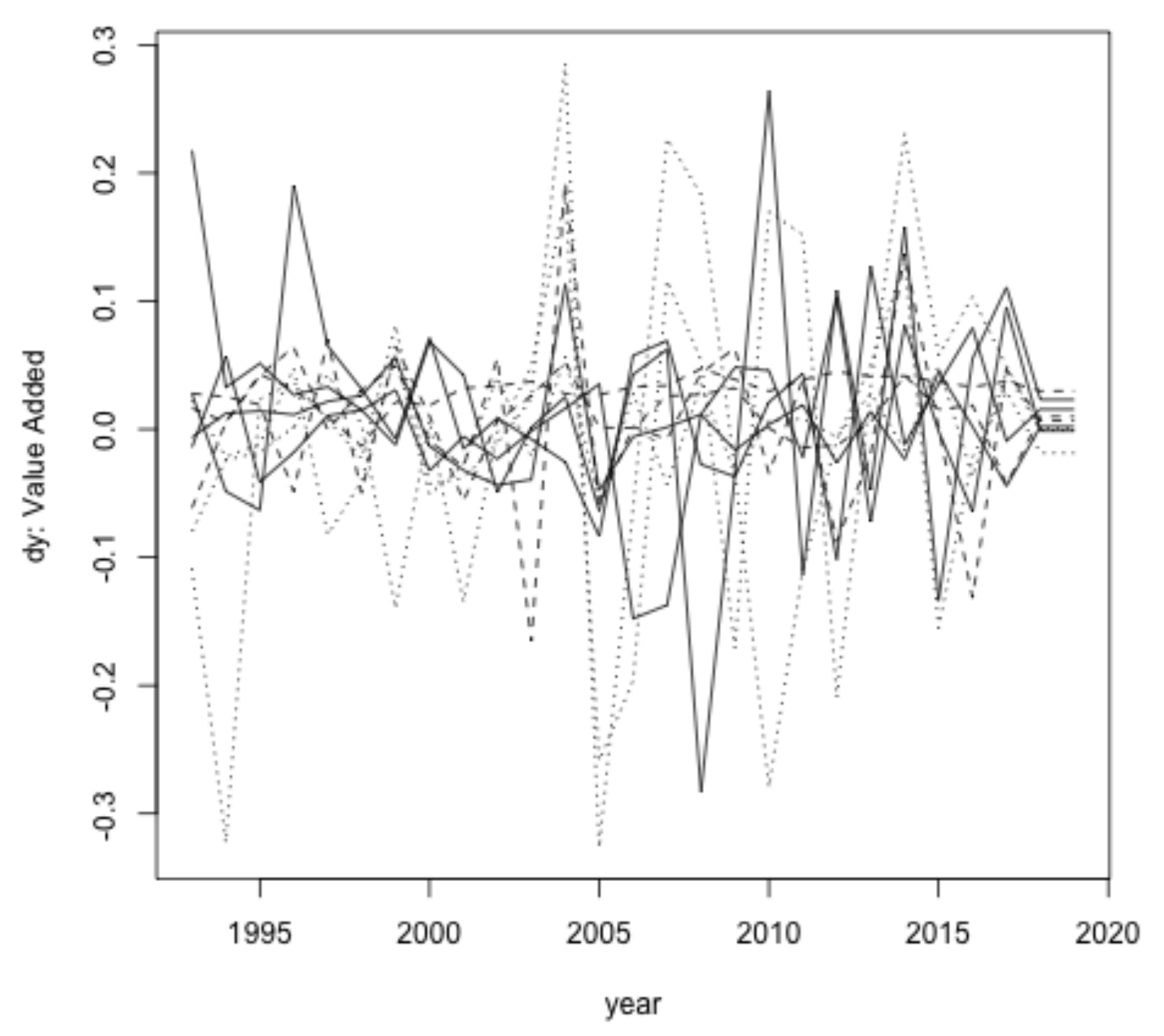
• Y: Value Added (Agriculture, Forestry and Fishing), in millions of USD, 2010 prices.
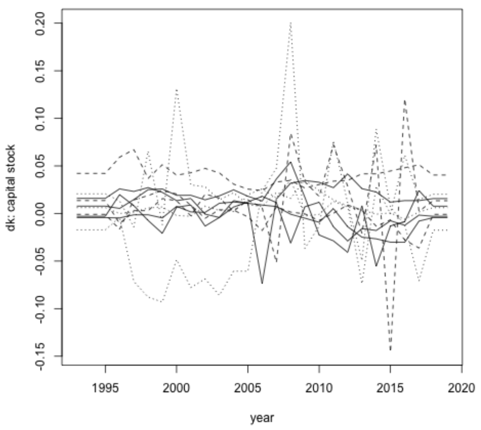
• K: Net Capital Stocks (Agriculture, Forestry and Fishing), in millions of USD, 2010 prices.
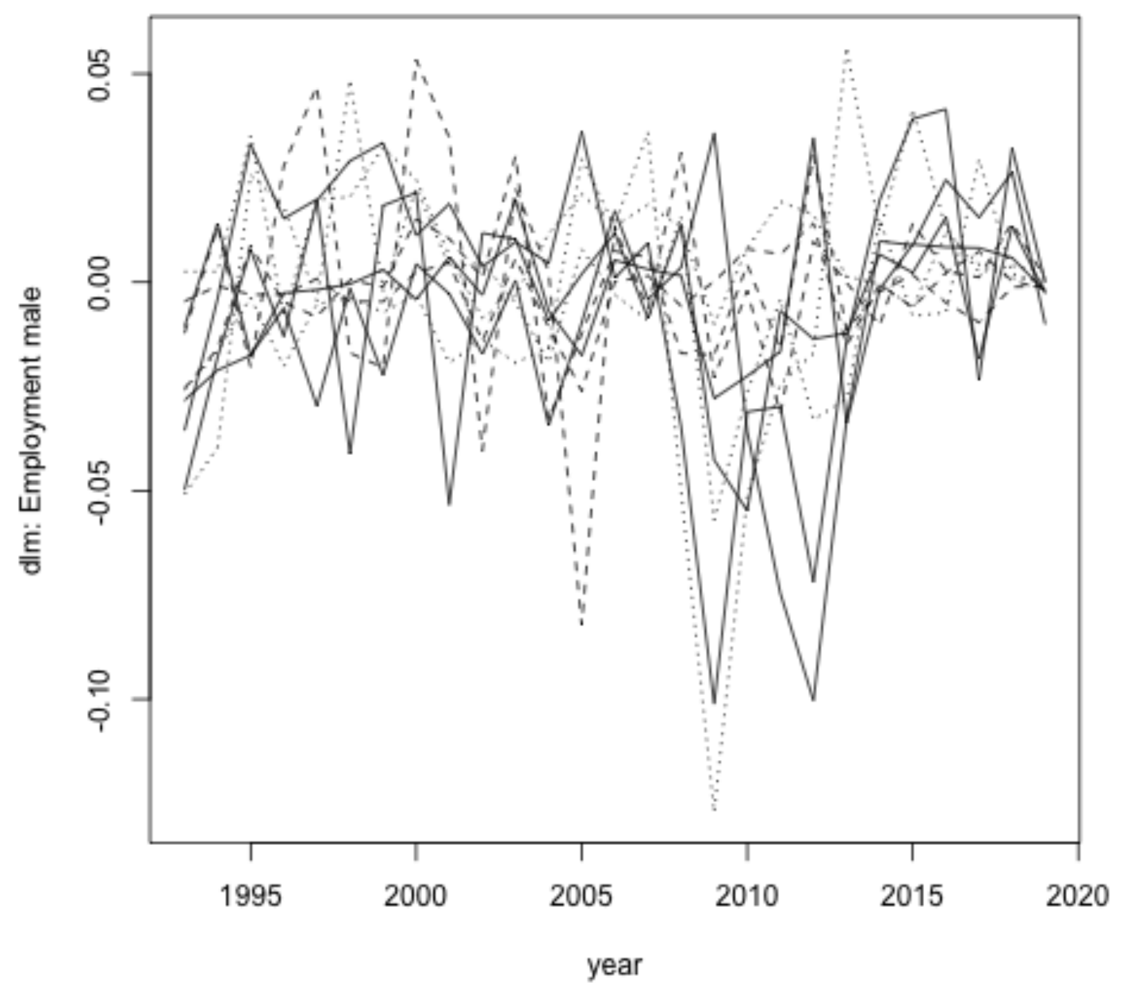
• $LM$: Employment-to-population ratio, rural areas, male, percentage.
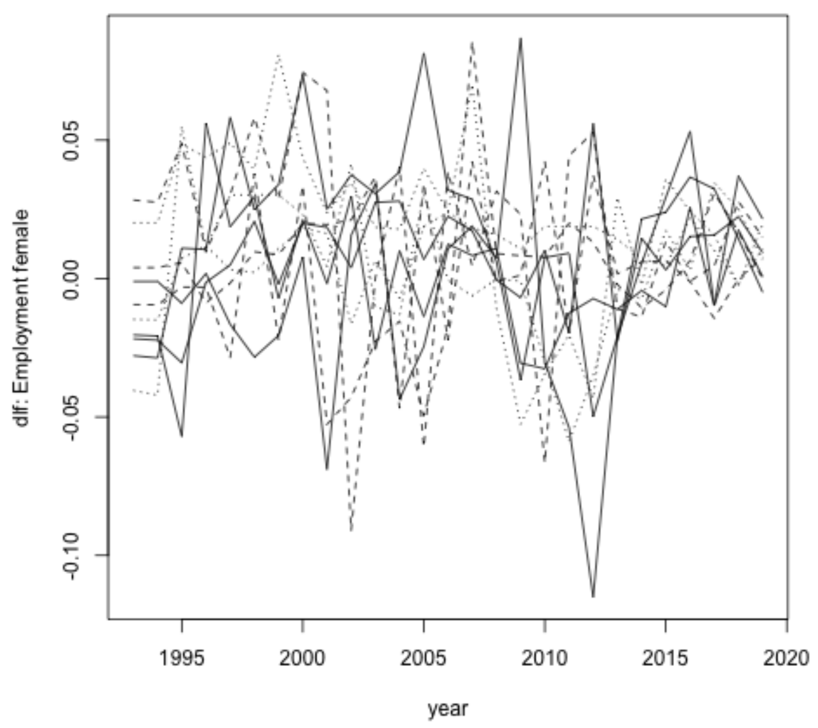
• $LF$: Employment-to-population ratio, rural areas, female, percentage.
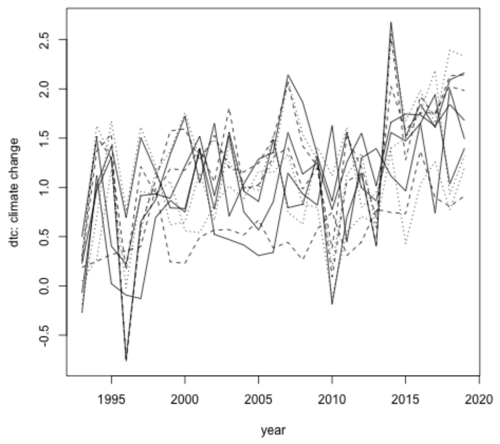
• $dtc$: Temperature change, during the meteorological year (°C).

The FAO NCS [57] is computed though the application of the perpetual inventory method (PIM) to agricultural investment flows variables contained in the FAO database (Gross Fixed Capital Formation (GFCF), Net (or Wealth), Capital Stock (NCS) and Consumption of Fixed Capital (CFC)). Those variables are measured according to the methodological and computational concepts of the System of National Accounts (SNA) 2008 (contrarialy to Cosculluela-Martínez (2020) [6] the complementary capital is not included to evaluate only the direct effects of the investement in those variables and exclude the possible impact on other capital stock types that could distortion the conclusions in this case).

Due to the absence of data from the total number of countries the analysis has been made for the period 1992 to 2019 of eleven countries: Denmark, France, Germany, Indonesia, Ireland, Italy, Netherlands, Portugal, Spain and United Kingdom.

3.2. Univariate Analysis

The Augmented Dickey–Fuller Test (ADF) (

Table 1. Augmented Dickey–Fuller Test p.values for first and second Differenced Series.

v.a.	ADF_p.Value	v.a.	ADF_p.Value
data_Denmark$dy	0.048	data_Denmark$dlm	0.423
data_France$dy	0.010	data_France$dlm	0.124
data_Germany$dy	0.010	data_Germany$dlm	0.422
data_Greece$dy	0.169	data_Greece$dlm	0.096
data_Indonesia$dy	0.099	data_Indonesia$dlm	0.365
data_Ireland$dy	0.109	data_Ireland$dlm	0.351
data_Italy$dy	0.028	data_Italy$dlm	0.071
data_Netherlands$dy	0.010	data_Netherlands$dlm	0.149
data_Portugal$dy	0.021	data_Portugal$dlm	0.610
data_Spain$dy	0.047	data_Spain$dlm	0.628
data_UK$dy	0.236	data_UK$dlm	0.109
data_Denmark$dlf	0.010	data_Denmark$dtc	0.303
data_France$dlf	0.515	data_France$dtc	0.751
data_Germany$dlf	0.141	data_Germany$dtc	0.252
data_Greece$dlf	0.090	data_Greece$dtc	0.253
data_Indonesia$dlf	0.263	data_Indonesia$dtc	0.465
data_Ireland$dlf	0.487	data_Ireland$dtc	0.528
data_Italy$dlf	0.159	data_Italy$dtc	0.307
data_Netherlands$dlf	0.381	data_Netherlands$dtc	0.370
data_Portugal$dlf	0.769	data_Portugal$dtc	0.266
data_Spain$dlf	0.449	data_Spain$dtc	0.474
data_UK$dlf	0.099	data_UK$dtc	0.686
data_Denmark$dk	0.210	diff(data_Denmark$dy)	0.010
data_France$dk	0.223	diff(data_France$dy)	0.010
data_Germany$dk	0.634	diff(data_Germany$dy)	0.010
data_Greece$dk	0.309	diff(data_Greece$dy)	0.021
data_Indonesia$dk	0.709	diff(data_Indonesia$dy)	0.010
data_Ireland$dk	0.578	diff(data_Ireland$dy)	0.010
data_Italy$dk	0.592	diff(data_Italy$dy)	0.010
data_Netherlands$dk	0.240	diff(data_Netherlands$dy)	0.010
data_Portugal$dk	0.230	diff(data_Portugal$dy)	0.010
data_Spain$dk	0.507	diff(data_Spain$dy)	0.010
data_UK$dk	0.344	diff(data_UK$dy)	0.013
diff(data_Denmark$dlm)	0.014	diff(data_Denmark$dlf)	0.010
diff(data_France$dlm)	0.010	diff(data_France$dlf)	0.070
diff(data_Germany$dlm)	0.112	diff(data_Germany$dlf)	0.010
diff(data_Greece$dlm)	0.077	diff(data_Greece$dlf)	0.047
diff(data_Indonesia$dlm)	0.037	diff(data_Indonesia$dlf)	0.010
diff(data_Ireland$dlm)	0.249	diff(data_Ireland$dlf)	0.183
diff(data_Italy$dlm)	0.010	diff(data_Italy$dlf)	0.030
diff(data_Netherlands$dlm)	0.010	diff(data_Netherlands$dlf)	0.033
diff(data_Portugal$dlm)	0.016	diff(data_Portugal$dlf)	0.104
diff(data_Spain$dlm)	0.336	diff(data_Spain$dlf)	0.258
diff(data_UK$dlm)	0.010	diff(data_UK$dlf)	0.010

and

Table 2. Augmented Dickey–Fuller Test p.values for first and second Differenced Series (cont.).

v.a.	ADF_p.value
diff(data_Denmark$dtc)	0.083
diff(data_France$dtc)	0.010
diff(data_Germany$dtc)	0.015
diff(data_Greece$dtc)	0.062
diff(data_Indonesia$dtc)	0.024
diff(data_Ireland$dtc)	0.170
diff(data_Italy$dtc)	0.010
diff(data_Netherlands$dtc)	0.027
diff(data_Portugal$dtc)	0.155
diff(data_Spain$dtc)	0.096
diff(data_UK$dtc)	0.151
diff(data_Denmark$dk)	0.010
diff(data_France$dk)	0.052
diff(data_Germany$dk)	0.189
diff(data_Greece$dk)	0.036
diff(data_Indonesia$dk)	0.050
diff(data_Ireland$dk)	0.031
diff(data_Italy$dk)	0.593
diff(data_Netherlands$dk)	0.020
diff(data_Portugal$dk)	0.096
diff(data_Spain$dk)	0.030
diff(data_UK$dk)	0.010

) shows that all the variables are stationary in the second differences of the natural logarithm, I(2). The results show that there is no over-differencing of the series, there are no MA terms in the univariate process followed by the variables (the literature suggest that series of Gross Added Value could be I(2), specially when considering partial (sectorized) Gross Added Value).

The graphical representation (Appendix A) shows that all the variables are I(1) except the climate change which seems to be I(2). Contrarialy the ADF test shows I(2) variables stationary in second differences of the level.

3.3. Cointegration

The Johansen cointegration test [58,59] shows that there is one cointegration relationship between the variables according to FPE order selection [53] in all the eleven countries (

Table 3. Lag Order.

	Denmark	France	Germany	Greece	Indonesia	Ireland	Italy	Netherlands	Portugal	Spain	UK
AIC(n)	4	4	4	4	4	4	4	4	4	4	4
HQ(n)	4	4	4	4	4	4	4	4	4	4	4
SC(n)	4	4	4	4	4	4	4	4	4	4	4
FPE(n)	4	4	3	4	3	3	4	3	4	4	3

).

3.4. Vectorial Estimation

The models are appropriate and correctly estimated, there is not enough evidence to reject the null hypotheses of serial autocorrelation or of the presence of no arch effects (heteroscedastycity) of the residuals of the VAR representation of the VEC estimations in I(2) variables for 2 lags and one cointegration equation. Thus, there is no cluster volatility in the model [60].

4. Results

Table 4. SRFs for dy (percentage).

	Denmark	France	Germany	Greece	Indonesia	Ireland	Netherlands	Italy	Portugal	Spain	UK
1	−0.6	−1.3	3.2	−2.2	0.0	−3.2	−0.8	−0.3	−1.7	−2.2	1.0
2	2.8	0.5	3.7	−0.8	−0.4	−4.7	−1.0	0.1	−0.4	−3.4	0.4
3	−4.3	−0.6	6.5	−1.2	−0.2	1.2	−0.3	−0.7	−1.8	−0.9	0.5
4	−1.1	0.0	0.1	−0.9	−0.5	−0.8	−1.0	−1.4	−0.4	−2.1	0.9
5	0.1	−0.4	1.9	−1.2	−0.2	−2.8	−0.5	−0.1	−1.4	−2.5	−0.7
6	−1.1	−0.2	5.4	−1.0	−0.3	−1.0	−0.8	−0.6	−0.9	−1.8	1.1
7	−1.9	−0.2	2.8	−1.1	−0.2	−0.7	−0.6	−0.9	−1.1	−1.7	0.7
8	−0.4	−0.2	2.9	−1.0	−0.3	−2.1	−0.8	−0.7	−1.0	−2.4	−0.3
9	−1.0	−0.2	2.6	−1.1	−0.3	−1.3	−0.6	−0.5	−1.1	−2.0	0.8
10	−1.2	−0.2	3.8	−1.1	−0.3	−0.9	−0.7	−0.6	−1.0	−1.8	0.9
11	−1.1	−0.2	3.3	−1.1	−0.3	−1.7	−0.7	−0.9	−1.1	−2.3	−0.4
12	−0.8	−0.2	2.5	−1.1	−0.3	−1.5	−0.7	−0.5	−1.0	−2.0	0.7
13	−1.1	−0.2	3.5	−1.1	−0.3	−1.1	−0.7	−0.7	−1.1	−1.9	0.9
14	−1.0	−0.2	3.2	−1.1	−0.3	−1.5	−0.7	−0.7	−1.0	−2.2	−0.1
15	−1.0	−0.2	3.1	−1.1	−0.3	−1.5	−0.7	−0.7	−1.1	−2.0	0.5

,

Table 5. SRFs for dlf (percentage).

	Denmark	France	Germany	Greece	Indonesia	Ireland	Netherlands	Italy	Portugal	Spain	UK
1	0.3	0.1	−0.2	−0.5	−0.2	−0.6	1.3	0.0	−0.5	−1.0	0.2
2	0.8	0.2	0.2	0.7	1.1	−0.2	0.3	0.7	−0.2	−1.2	0.0
3	0.6	0.2	0.1	0.4	−0.1	−0.3	0.3	−0.3	−0.4	−1.0	−0.2
4	0.6	0.1	0.1	0.7	0.4	−0.4	0.7	0.1	−0.4	−0.9	0.5
5	0.3	0.2	0.1	0.5	0.3	−0.6	0.4	0.1	−0.2	−1.0	−0.2
6	0.8	0.2	0.1	0.5	0.9	−0.3	0.5	0.1	−0.4	−1.1	0.1
7	0.5	0.2	0.2	0.6	0.1	−0.4	0.5	0.0	−0.3	−0.9	−0.1
8	0.6	0.2	0.0	0.6	0.3	−0.5	0.4	0.0	−0.3	−1.0	0.1
9	0.5	0.2	0.1	0.6	0.4	−0.4	0.5	0.2	−0.3	−1.1	0.0
10	0.6	0.2	0.1	0.6	0.5	−0.4	0.5	0.0	−0.3	−0.9	0.0
11	0.5	0.2	0.1	0.6	0.3	−0.4	0.5	0.1	−0.3	−1.0	0.0
12	0.6	0.2	0.1	0.6	0.3	−0.4	0.5	0.0	−0.3	−1.0	0.1
13	0.6	0.2	0.1	0.6	0.4	−0.4	0.5	0.1	−0.3	−1.0	−0.1
14	0.6	0.2	0.1	0.6	0.4	−0.4	0.5	0.0	−0.3	−1.0	0.0
15	0.6	0.2	0.1	0.6	0.3	−0.4	0.5	0.1	−0.3	−1.0	0.1

,

Table 6. SRFs for dlm (percentage).

	Denmark	France	Germany	Greece	Indonesia	Ireland	Netherlands	Italy	Portugal	Spain	UK
1	0.3	0.1	0.6	0.7	0.1	−0.2	−1.0	0.1	0.5	−1.4	0.3
2	−0.1	−0.1	0.2	1.2	0.2	−0.4	−0.9	0.3	−0.4	−2.0	0.3
3	0.6	−0.1	0.0	1.1	0.0	−0.3	−0.7	−0.6	0.2	−1.3	−0.3
4	0.6	0.0	0.4	1.3	−0.1	−0.6	−0.8	−0.3	0.1	−1.2	0.6
5	0.0	−0.1	0.2	1.2	0.2	−0.7	−0.8	−0.1	0.0	−1.6	0.0
6	0.5	−0.1	0.2	1.2	0.1	−0.3	−0.7	−0.2	0.1	−1.6	0.1
7	0.4	0.0	0.2	1.2	0.1	−0.4	−0.8	−0.3	0.1	−1.2	0.0
8	0.3	−0.1	0.2	1.2	0.0	−0.6	−0.8	−0.3	0.0	−1.5	0.3
9	0.3	−0.1	0.3	1.2	0.1	−0.4	−0.8	−0.1	0.1	−1.5	0.0
10	0.4	−0.1	0.2	1.2	0.1	−0.4	−0.8	−0.3	0.0	−1.3	0.1
11	0.3	−0.1	0.2	1.2	0.1	−0.5	−-0.8	−0.2	0.1	−1.5	0.2
12	0.3	−0.1	0.2	1.2	0.1	−0.5	−0.8	−0.2	0.0	−1.5	0.2
13	0.3	−0.1	0.2	1.2	0.1	−0.4	−0.8	−0.2	0.1	−1.4	0.0
14	0.4	−0.1	0.2	1.2	0.1	−0.5	−0.8	−0.3	0.0	−1.5	0.2
15	0.3	−0.1	0.2	1.2	0.1	−0.5	−0.8	−0.3	0.1	−1.5	0.1

,

Table 7. SRFs for dtc (percentage).

	Denmark	France	Germany	Greece	Indonesia	Ireland	Netherlands	Italy	Portugal	Spain	UK
1	−15.9	20.3	24.5	18.3	0.2	−10.7	28.2	4.0	9.7	−10.2	17.8
2	−6.6	0.4	25.0	14.6	8.0	−3.5	6.3	0.0	3.5	−10.8	5.1
3	−0.9	11.4	3.0	16.0	3.3	−11.8	18.9	−13.7	4.8	−3.7	11.4
4	5.4	7.2	16.5	16.4	6.8	−5.6	12.7	−9.8	9.8	−10.0	11.0
5	−10.4	8.1	18.4	16.3	3.1	−9.5	16.4	−4.1	1.9	−7.8	6.8
6	−1.3	8.1	20.3	16.0	1.0	−8.4	13.1	−6.7	8.4	−7.0	10.3
7	−0.7	8.2	4.0	16.1	3.2	−7.8	16.3	−11.2	5.0	−8.3	11.2
8	−2.9	7.9	18.2	16.2	4.6	−7.9	13.7	−7.2	6.3	−7.5	8.4
9	−4.2	8.1	18.4	16.1	4.6	−8.8	15.5	−5.1	5.6	−7.9	9.0
10	−1.2	8.1	11.9	16.1	3.0	−7.9	14.4	−9.5	6.4	−7.9	11.8
11	−2.8	8.0	14.9	16.1	3.6	−8.0	15.0	−8.2	5.5	−7.3	8.1
12	−2.8	8.1	13.9	16.1	3.7	−8.4	14.6	−7.2	6.2	−8.3	8.9
13	−2.7	8.1	17.3	16.1	3.6	−8.2	14.9	−6.8	5.8	−7.5	11.7
14	−2.2	8.1	13.3	16.1	3.4	−8.0	14.7	−8.9	6.0	−7.5	8.6
15	−2.8	8.1	13.9	16.1	3.8	−8.3	14.9	−7.7	5.9	−8.2	8.8

and

Table 8. SRFs for k (percentage).

	Denmark	France	Germany	Greece	Indonesia	Ireland	Netherlands	Italy	Portugal	Spain	UK
1	1.0	1.2	0.8	1.4	0.6	3.5	4.7	0.7	3.5	1.7	1.5
2	1.0	1.1	0.5	0.9	0.4	1.8	1.0	0.7	1.2	0.9	0.1
3	0.5	1.1	0.2	1.3	0.4	3.5	4.2	0.7	2.9	0.7	0.3
4	0.6	1.0	0.4	1.1	0.2	3.5	1.8	0.8	1.6	1.1	0.8
5	0.9	1.1	0.6	1.1	0.3	2.5	3.3	0.8	2.6	1.1	1.1
6	0.7	1.1	0.3	1.1	0.3	2.6	2.5	0.7	1.9	0.8	0.4
7	0.7	1.1	0.4	1.2	0.3	3.3	2.9	0.7	2.3	1.0	0.7
8	0.7	1.1	0.4	1.1	0.3	2.8	2.7	0.8	2.0	1.0	0.8
9	0.7	1.1	0.5	1.2	0.3	2.7	2.9	0.8	2.3	0.9	0.6
10	0.7	1.1	0.4	1.2	0.3	3.1	2.7	0.8	2.1	1.0	0.7
11	0.7	1.1	0.4	1.2	0.3	2.9	2.8	0.8	2.2	1.0	0.8
12	0.7	1.1	0.5	1.2	0.3	2.8	2.8	0.8	2.1	1.0	0.7
13	0.7	1.1	0.4	1.2	0.3	3.0	2.8	0.8	2.2	1.0	0.7
14	0.7	1.1	0.4	1.2	0.3	2.9	2.8	0.8	2.2	1.0	0.7
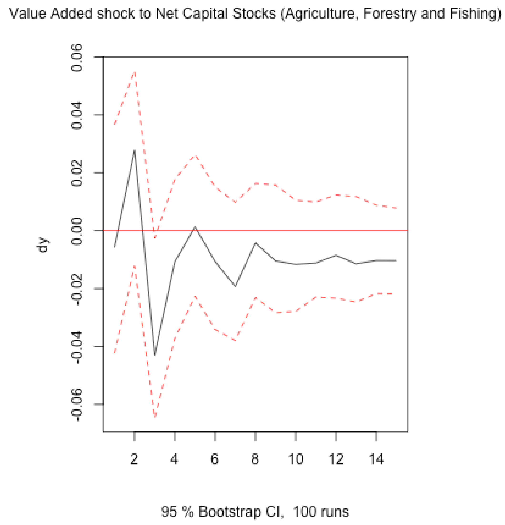
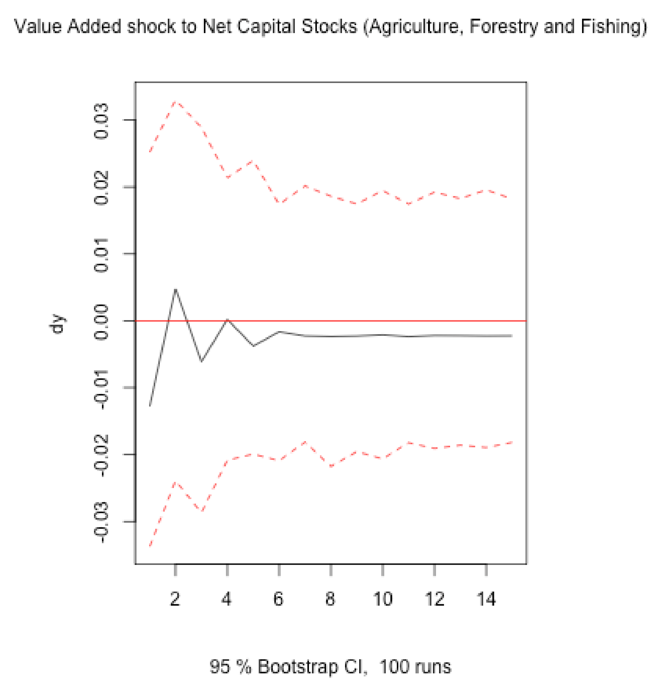
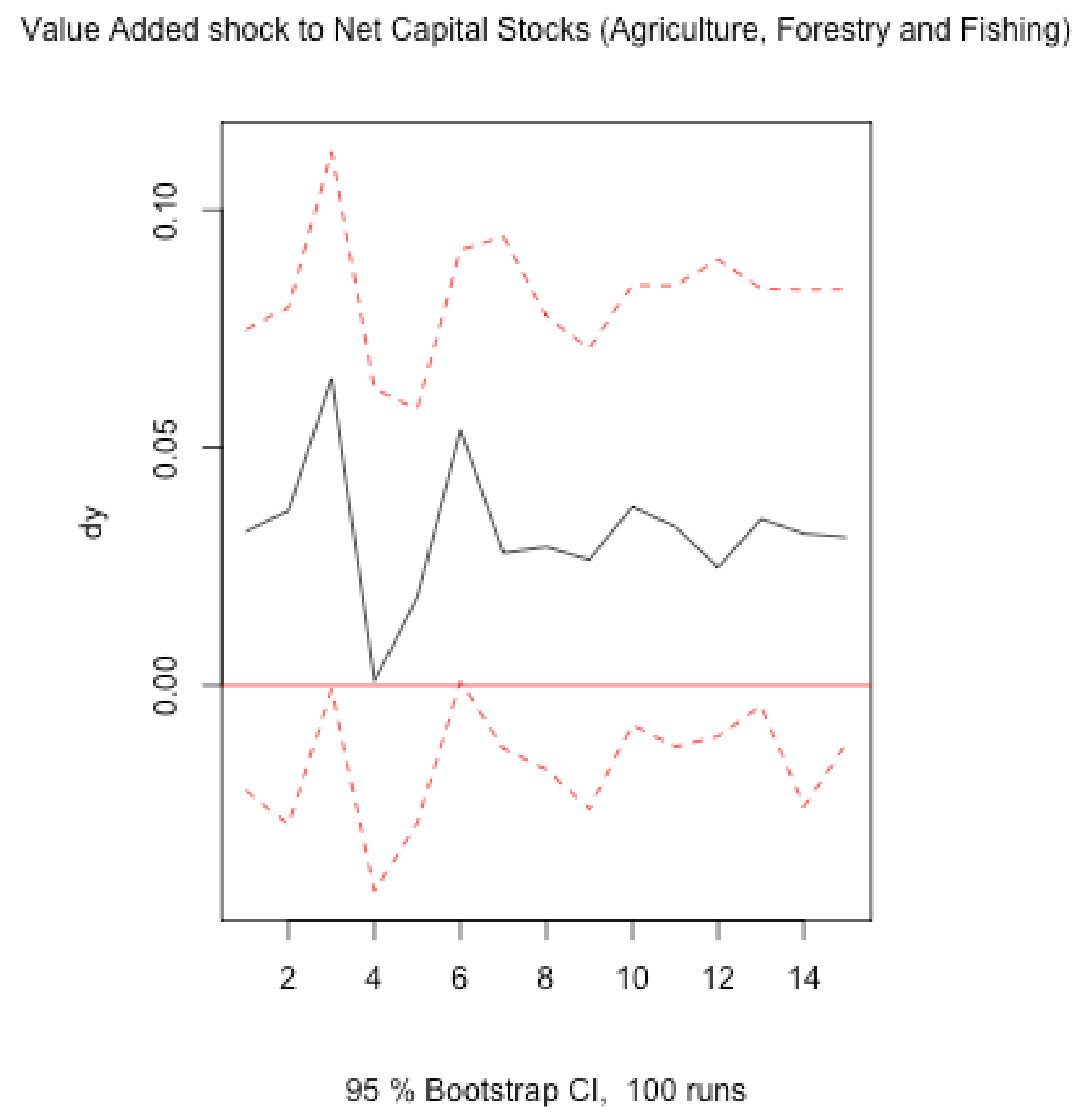
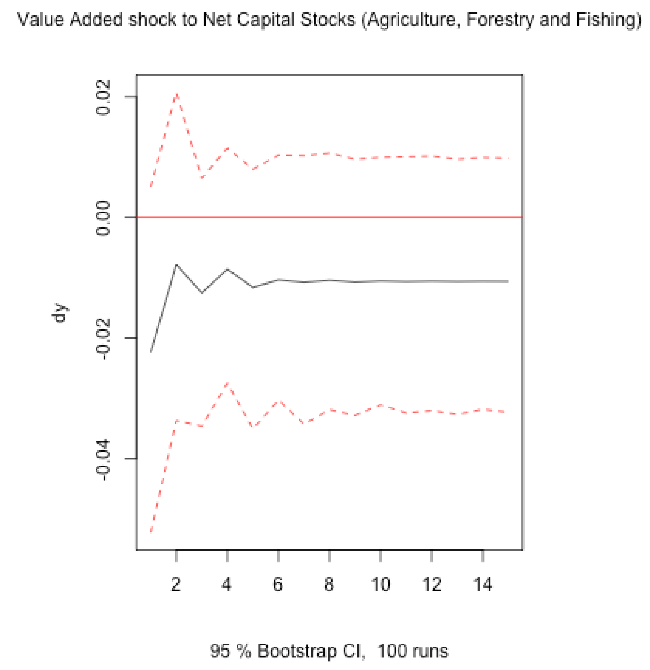
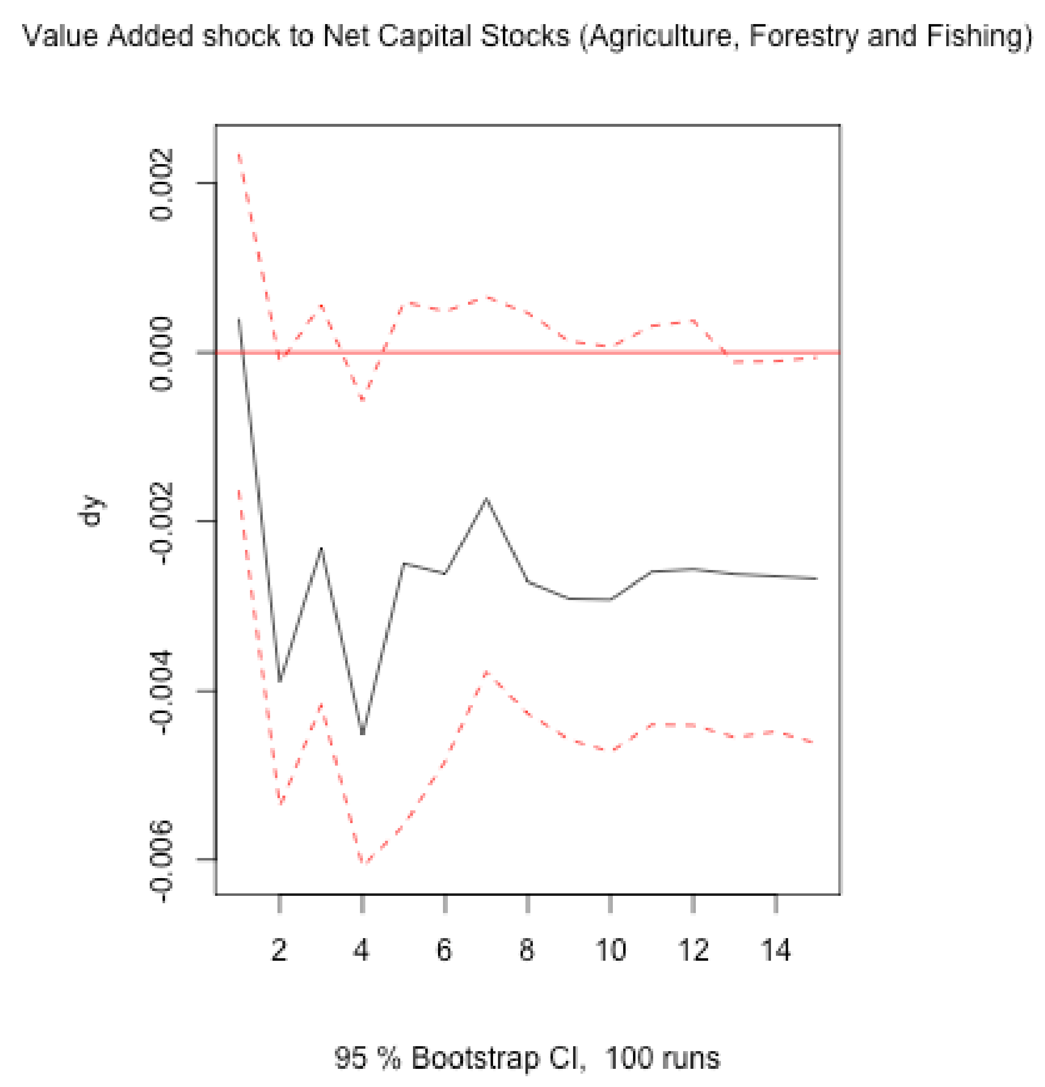
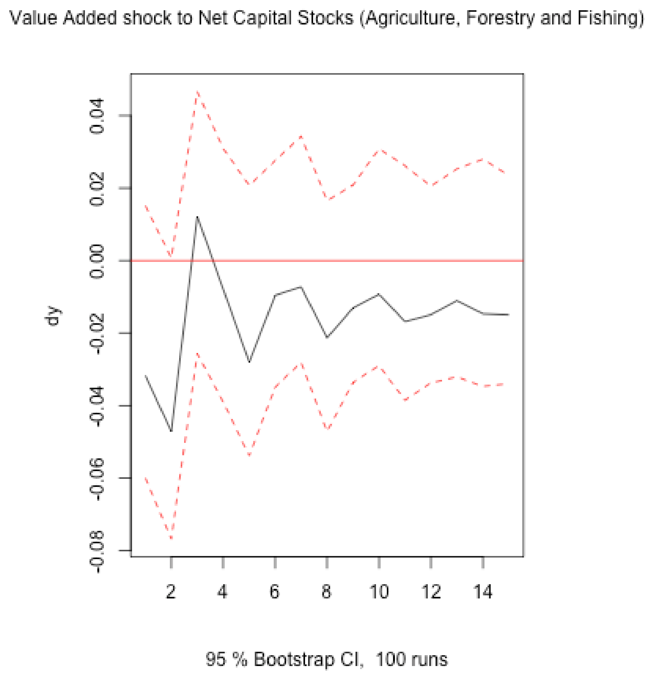
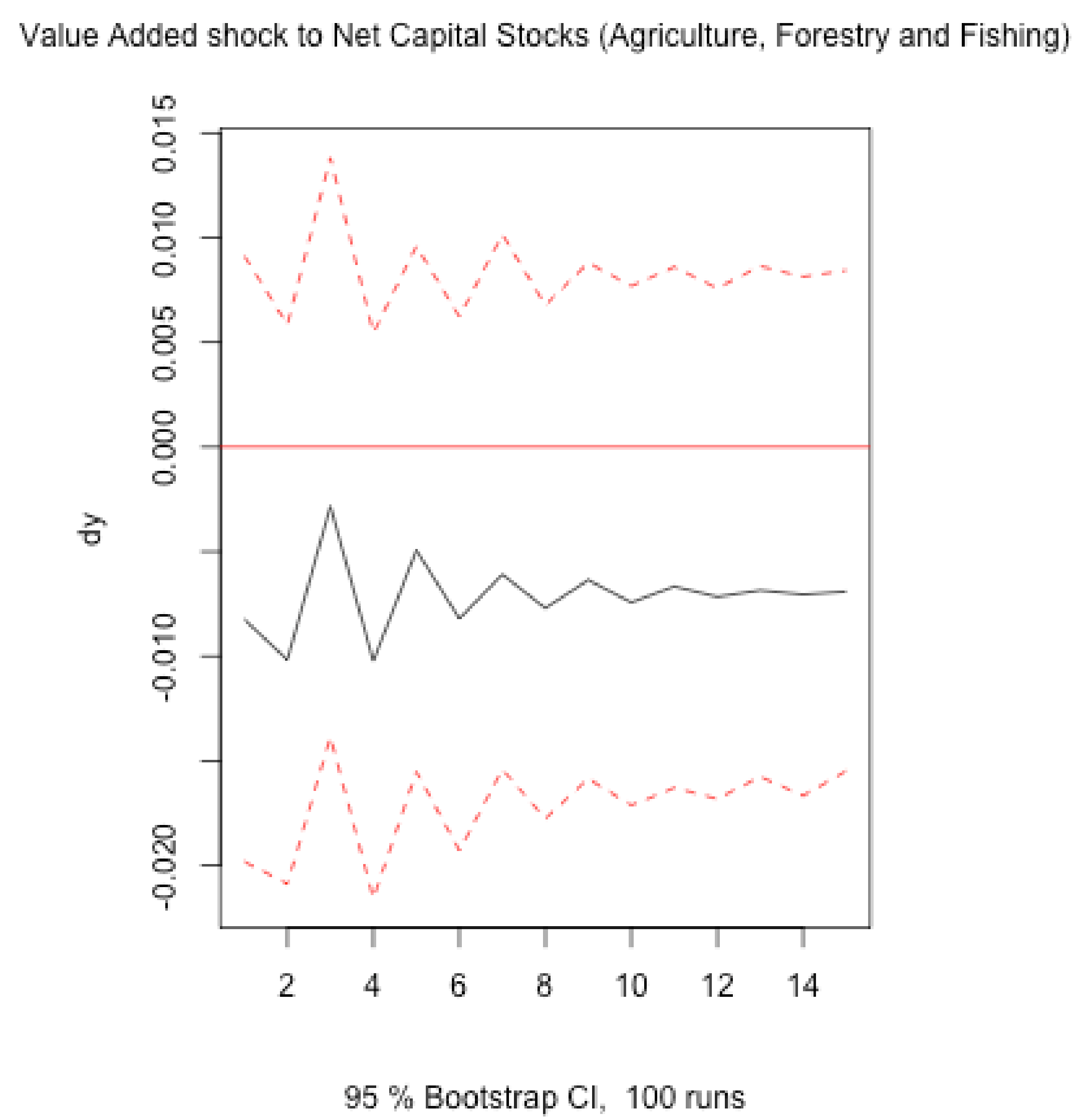
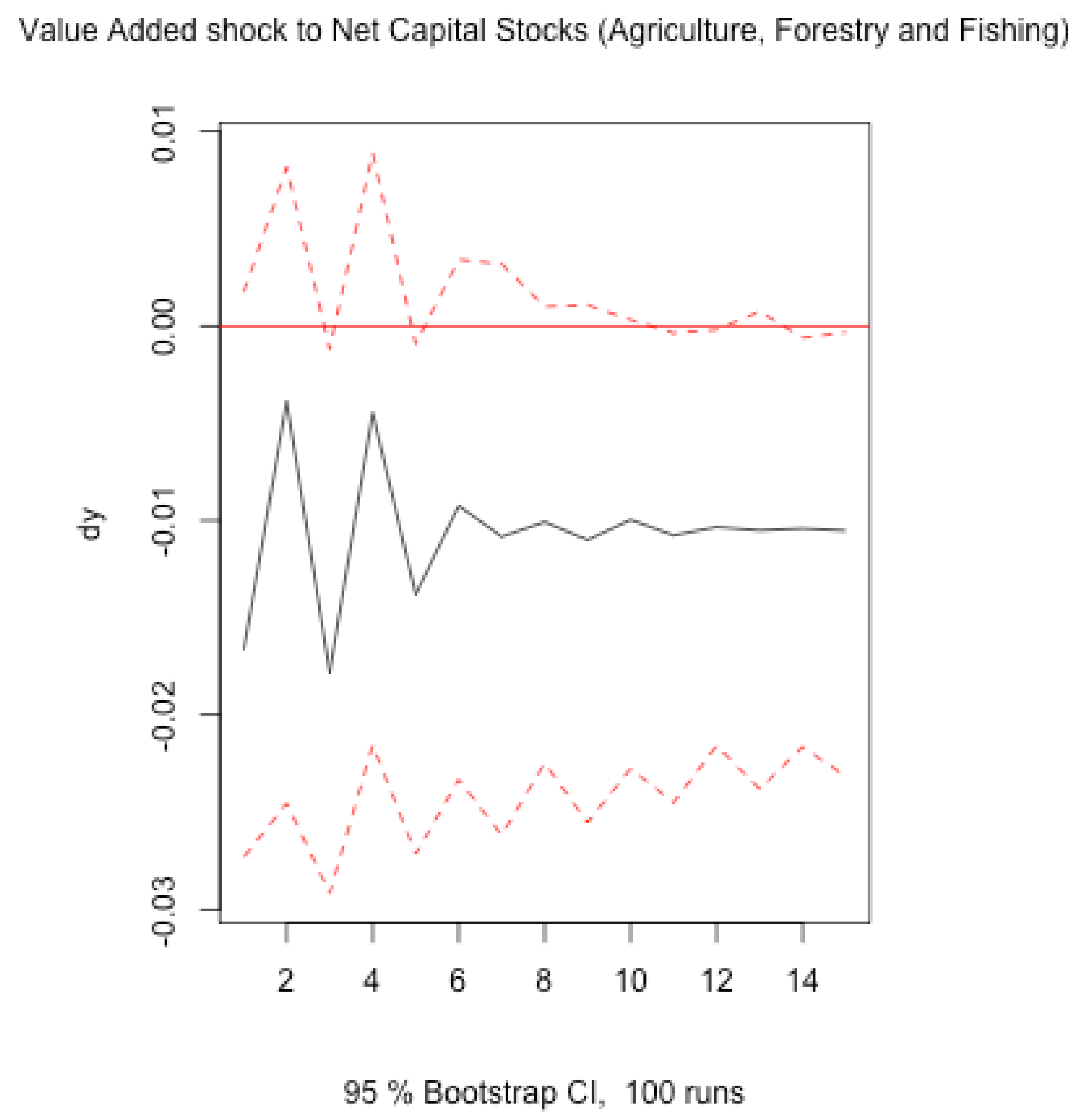
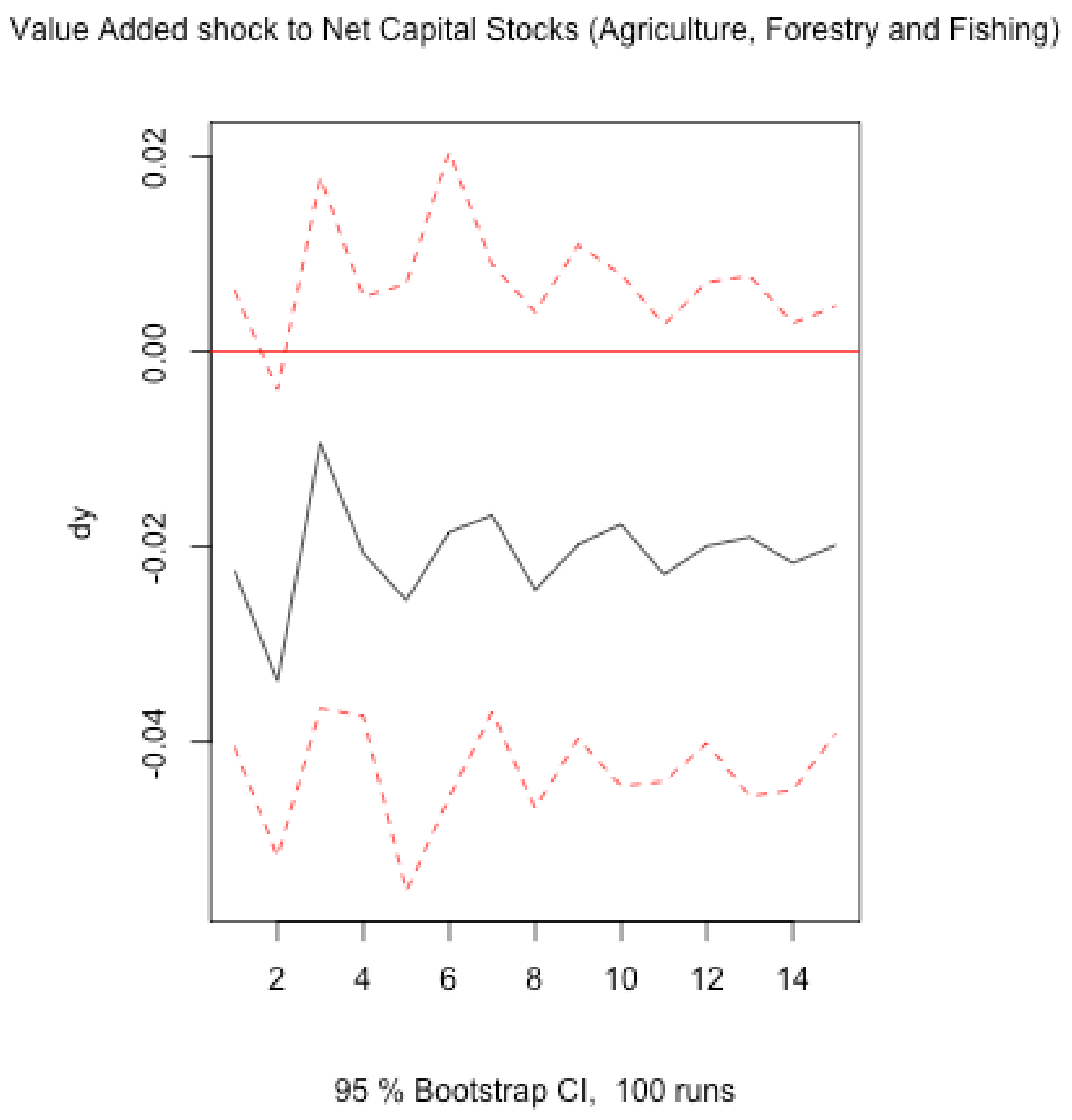
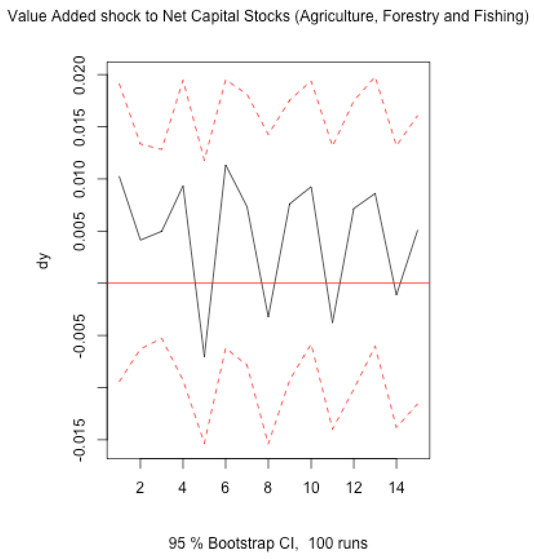
15	0.7	1.1	0.4	1.2	0.3	2.8	2.8	0.8	2.2	1.0	0.7

shows the estimated orthogonal step responses of value added growth, employment to population ratio in the rural areas growth -male and female- and rate of growth of climate change and feedback effects for each of the following 15 periods to the impulse in the rate of growth of the NCS (Agriculture, Forestry and Fishing), which is a one standard deciation increase in the level of the NCS.

The orthogonalided SRFs to a shock in NCS, a forecast error impulse K, a structural increase of NCS, reveal:

First, the value added rate of growth only increases in the second period after the shock in Germany. Denmark, France, Germany, Italy and UK, increase the rate of growth of value added. The rate of growth is directly and negatively affected by the increase in NCS for the agriculture, forestry and fishing except in Germany and UK. The purpose of the paper was ti examine the direct effects of the particular investment, and possibly the absence of the complementary capital and the effects of the capital stock for the Agriculture, Forestry and Fishing on it could exponentially cause positive effects on output as the literature reveals.

Second, the effect on the rate of growth of the ratio of employed female to population increases in all the countries except Ireland, Portugal and Spain. Contrarily reduces the rate of growth of the employed men to population ratio in France, Ireland, Netherlands, Italy and Spain.

Third, temperature change is affected negatively by the increase in NCS in Denmark, Ireland, Italy and Spain. The results suggest that depending on the country an increase in NCS can affect directly changes in the temperature. France, Germany Greece and Netherlands present the most positive effects while Denmark, Ireland and Spain reveal the most negative ones.

Fourth, the analysis reveals that the investment crowds in investment. There is an increase during all the time span considered of net capital.

5. Conclusions

The paper examines the effect of an increase in NCS for agriculture, forestry, and fishing in gender gap drop-down in employment and climate change. The methodology used is the computed SRFs from the estimated VECMs conveniently orthogonalized to avoid instant sensitivity of the net capital to changes in the rest of the variables.

The investment of NCS reduces the gender gap in employment in rural areas in eight of the eleven countries studied: Denmark, France, Germany, Greece, Indonesia, Netherlands, Italy, and the UK. Answering the first hypothesis, “Some countries have much higher gender gap drop-down due to the investment in NCS (agriculture, forestry, and fishing).” The results conclude that a gender gap drop-down can be observed due to an investment in capital for agriculture, forestry, and fishing in all countries except Ireland, Portugal, and Spain. In Spain, the investment reduces the ratios of employment versus population growth. In France, Ireland, Netherlands, and Italy, the drop-down in the ratio employed males divided by population can be explained by an increase of the population in the agricultural sector greater than the increase in the male population employed, or by the natural substitution of employment by machinery. Thus, it is a very powerful instrument to achieve an important feature of the SDG 2.4; it increases employed women more than the rural population in 8 of 11 countries, while it increases fewer men employed than the population in rural areas in almost half of the countries (five out of eleven). Besides, as commented in the discussion section, gender equality favors agricultural transformation and sustainability contributing to mitigate climate change.

Contrarily, there is not a clear conclusion on the effect of climate change. Depending on the country, the direct effect can be highly negative or extremely positive. Intelligent machinery to be productive and efficient is supposed to increase contamination and temperature change. Nevertheless, according to the results obtained, the second hypothesis is not conclusive “Long-run effects on climate change are present in all the countries when increasing NCS for the agriculture, forestry, and fishing.”

The third hypothesis, “Which countries have the higher climate reverse effect investing a one percentage point in NCS (agriculture, forestry, and fishing)” can be answered by naming three Greece, Netherlands, and Germany.

According to the literature, the results reveal that capital crowds in the capital. The results of the paper reveal that weighting European Funds in intelligent, sustainable Technology for agriculture, fishing, and forestry is a very powerful macroeconomic instrument to achieve the SDG 2.4. A limitation of the study is to analyze the complete (total) effect of the investment, considering as another variable all the complementary capital, which will give a much more exponential effect on output and gender gap drop-down.

References

1. FAO. Agricultural Investments and Capital Stock; Technical Report; FAO: Rome, Italy, 2020. [Google Scholar]
2. Bryan, E. A Focus on Gender is Key to Climate Adaptation; International Food Policy Research Institute: Washington, DC, USA, 2019. [Google Scholar]
3. FAO. World Livestock: Transforming the Livestock Sector Through the Sustainable Development Goals; Technical Report; FAO: Rome, Italy, 2018. [Google Scholar]
4. Ignaciuk, A.; Chit Tun, N.A. Achieving Agricultural Sustainability Depends on Gender Equality; International Food Policy Research Institute: Washington, DC, USA, 2019. [Google Scholar]
5. Hudson, R.J. Animal and Plant Productivity; Eolss Publications: Abu Dhabi, United Arab Emirates, 2010; Volume 10. [Google Scholar]
6. Cosculluela-Martinez, C. Sustainable Knowledge Investment Increases Employment and GDP in the Spanish Agricultural Sector More Than Other Investments. Sustainability 2020, 12, 3127. [Google Scholar] [CrossRef] [Green Version]
7. Aschauer, D.A. Is public expenditure productive? J. Monet. Econ. 1989, 23, 177–200. [Google Scholar] [CrossRef]
8. Aschauer, D.A. Public investment and productivity growth in the Group of Seven. Econ. Perspect. 1989, 13, 17–25. [Google Scholar]
9. Aschauer, D.A. Does public capital crowd out private capital? J. Monet. Econ. 1989, 24, 171–188. [Google Scholar] [CrossRef]
10. Fedele, G.; Donatti, C.I.; Harvey, C.A.; Hannah, L.; Hole, D.G. Limited use of transformative adaptation in response to social-ecological shifts driven by climate change. Ecol. Soc. 2020, 25, 25. [Google Scholar] [CrossRef] [Green Version]
11. Revi, A.; Satterthwaite, D.; Aragón-Durand, F.; Corfee-Morlot, J.; Kiunsi, R.B.; Pelling, M.; Roberts, D.; Solecki, W.; Gajjar, S.P.; Sverdlik, A. Towards transformative adaptation in cities: The IPCC’s Fifth Assessment. Environ. Urban. 2014, 26, 11–28. [Google Scholar] [CrossRef]
12. Aldieri, L.; Makkonen, T.; Vinci, C.P. Environmental knowledge spillovers and productivity: A patent analysis for large international firms in the energy, water and land resources fields. Resour. Policy 2020, 69, 101877. [Google Scholar] [CrossRef]
13. Wang, H.; Huang, J.; Zhou, H.; Deng, C.; Fang, C. Analysis of sustainable utilization of water resources based on the improved water resources ecological footprint model: A case study of Hubei Province, China. J. Environ. Manag. 2020, 262, 110331. [Google Scholar] [CrossRef]
14. Vander Donckt, M.; Chan, P. The New Fao Global Database on Agriculture Investment and Capital Stock. Available online: http://www.fao.org/3/ca6133en/CA6133EN.pdf (accessed on 1 February 2021).
15. Vander Donckt, M.; Chan, P.; Silvestrini, A. A new global database on agriculture investment and capital stock. Food Policy 2020, 100, 101961. [Google Scholar] [CrossRef]
16. Akbar, M.; Niaz, R.; Amjad, M. Determinants of households’ food insecurity with severity dimensions in Pakistan: Varying estimates using partial proportional odds model. Health Soc. Care Community 2020, 28, 1698–1709. [Google Scholar] [CrossRef]
17. Asumadu-Sarkodie, S.; Owusu, P.A. The relationship between carbon dioxide and agriculture in Ghana: A comparison of VECM and ARDL model. Environ. Sci. Pollut. Res. 2016, 23, 10968–10982. [Google Scholar] [CrossRef]
18. Asumadu-Sarkodie, S.; Owusu, P.A. The causal nexus between carbon dioxide emissions and agricultural ecosystem—An econometric approach. Environ. Sci. Pollut. Res. 2017, 24, 1608–1618. [Google Scholar] [CrossRef]
19. Engle, R.F. Autoregressive conditional heteroscedasticity with estimates of the variance of United Kingdom inflation. Econom. J. Econom. Soc. 1982, 50, 987–1007. [Google Scholar] [CrossRef]
20. Hamilton, J. Time Series Econometrics; Princeton University Press: Princeton, NJ, USA, 1994. [Google Scholar]
21. Lütkepohl, H. Structural vector autoregressive analysis for cointegrated variables. Allg. Stat. Arch. 2006, 90, 75–88. [Google Scholar]
22. Breusch, T.S. Testing for autocorrelation in dynamic linear models. Aust. Econ. Pap. 1978, 17, 334–355. [Google Scholar] [CrossRef]
23. Edgerton, D.; Shukur, G. Testing autocorrelation in a system perspective testing autocorrelation. Econom. Rev. 1999, 18, 343–386. [Google Scholar] [CrossRef]
24. Flores de Frutos, R.; Gracia-Díez, M.; Perez, T. Public capital stock and economic growth: An analysis of the Spanish economy. Appl. Econ. 1998, 30, 985–994. [Google Scholar] [CrossRef]
25. Cosculluela-Martínez, C.; de Frutos, R.F. Housing investment in Spain: Has it been the main engine of growth? Appl. Econ. 2013, 45, 1835–1843. [Google Scholar] [CrossRef] [Green Version]
26. Narzo, A.F.D.; Aznarte, J.L.; Stigler, M.; Tsung-wu, H. tsDyn: Nonlinear Time Series Models with Regime Switching. R Package Version 10-1. 2020. Available online: https://cran.r-project.org/web/packages/tsDyn/index.html (accessed on 1 February 2021).
27. Wickham, H. Forcats: Tools for Working with Categorical Variables (Factors). R Package Version 0.5.0. 2020. Available online: https://cran.r-project.org/web/packages/forcats/index.html (accessed on 1 February 2021).
28. Wickham, H. Stringr: Simple, Consistent Wrappers for Common String Operations. R Package Version 1.4.0. 2019. Available online: https://cran.r-project.org/web/packages/stringr/index.html (accessed on 1 February 2021).
29. Wickham, H.; François, R.; Henry, L.; Müller, K. Dplyr: A Grammar of Data Manipulation. R Package Version 1.0.2. 2020. Available online: https://cran.r-project.org/web/packages/dplyr/index.html (accessed on 1 February 2021).
30. Henry, L.; Wickham, H. Purrr: Functional Programming Tools. R Package Version 0.3.4. 2020. Available online: https://cran.r-project.org/web/packages/purrr/index.html (accessed on 1 February 2021).
31. Wickham, H.; Hester, J. Readr: Read Rectangular Text Data. R Package Version 1.4.0. 2020. Available online: https://cran.r-project.org/web/packages/readr/index.html (accessed on 1 February 2021).
32. Wickham, H. Tidyr: Tidy Messy Data. R Package Version 1.1.2. 2020. Available online: https://cran.r-project.org/web/packages/tidyr/index.html (accessed on 1 February 2021).
33. Müller, K.; Wickham, H. Tibble: Simple Data Frames. R Package Version 3.0.4. 2020. Available online: https://cran.r-project.org/web/packages/tibble/index.html (accessed on 1 February 2021).
34. Wickham, H.; Chang, W.; Henry, L.; Pedersen, T.L.; Takahashi, K.; Wilke, C.; Woo, K.; Yutani, H.; Dunnington, D. Ggplot2: Create Elegant Data Visualisations Using the Grammar of Graphics. R Package Version 3.3.2. 2020. Available online: https://cran.r-project.org/web/packages/ggplot2/index.html (accessed on 1 February 2021).
35. Wickham, H. Tidyverse: Easily Install and Load the Tidyverse. R Package Version 1.3.0. 2019. Available online: https://cran.r-project.org/web/packages/tidyverse/index.html (accessed on 1 February 2021).
36. Zhu, H. KableExtra: Construct Complex Table with kable and Pipe Syntax. R Package Version 1.3.1. 2020. Available online: https://cran.r-project.org/web/packages/kableExtra/index.html (accessed on 1 February 2021).
37. Wickham, H.; Bryan, J. Readxl: Read Excel Files. R Package Version 1.3.1. 2019. Available online: https://cran.r-project.org/web/packages/readxl/index.html (accessed on 1 February 2021).
38. Hyndman, R.; Athanasopoulos, G.; Bergmeir, C.; Caceres, G.; Chhay, L.; O’Hara-Wild, M.; Petropoulos, F.; Razbash, S.; Wang, E.; Yasmeen, F. forecast: Forecasting Functions for Time Series and Linear Models. R Package Version 8.13. 2020. Available online: https://cran.r-project.org/web/packages/forecast/forecast.pdf (accessed on 1 February 2021).
39. Xie, Y. Knitr: A General-Purpose Package for Dynamic Report Generation in R. R Package Version 1.31. 2021. Available online: https://cran.r-project.org/web/packages/knitr/index.html (accessed on 1 February 2021).
40. Fox, J.; Weisberg, S.; Price, B. Car: Companion to Applied Regression. R Package Version 3.0-10. 2020. Available online: https://cran.r-project.org/web/packages/car/index.html (accessed on 1 February 2021).
41. Fox, J.; Weisberg, S.; Price, B. carData: Companion to Applied Regression Data Sets. R Package Version 3.0-4. 2020. Available online: https://cran.r-project.org/web/packages/carData/index.html (accessed on 1 February 2021).
42. Robinson, D.; Hayes, A.; Couch, S. Broom: Convert Statistical Objects into Tidy Tibbles. R Package Version 0.7.2. 2020. Available online: https://cran.r-project.org/web/packages/broom/index.html (accessed on 1 February 2021).
43. Komashko, O. nlWaldTest: Wald Test of Nonlinear Restrictions and Nonlinear CI. R Package Version 1.1.3. 2016. Available online: https://cran.r-project.org/web/packages/nlWaldTest/index.html (accessed on 1 February 2021).
44. Pfaff, B. Vars: VAR Modelling. R Package Version 1.5-3. 2018. Available online: https://cran.r-project.org/web/packages/vars/index.html (accessed on 1 February 2021).
45. Hothorn, T.; Zeileis, A.; Farebrother, R.W.; Cummins, C. Lmtest: Testing Linear Regression Models. R Package Version 0.9-38. 2020. Available online: https://cran.r-project.org/web/packages/lmtest/index.html (accessed on 1 February 2021).
46. Pfaff, B. Urca: Unit Root and Cointegration Tests for Time Series Data. R Package Version 1.3-0. 2016. Available online: https://cran.r-project.org/web/packages/urca/index.html (accessed on 1 February 2021).
47. Zeileis, A.; Leisch, F.; Hornik, K.; Kleiber, C. Strucchange: Testing, Monitoring, and Dating Structural Changes. R Package Version 1.5-2. 2019. Available online: https://cran.r-project.org/web/packages/strucchange/index.html (accessed on 1 February 2021).
48. Zeileis, A.; Lumley, T. Sandwich: Robust Covariance Matrix Estimators. R Package Version 3.0-0. 2020. Available online: https://cran.r-project.org/web/packages/sandwich/index.html (accessed on 1 February 2021).
49. Ripley, B. MASS: Support Functions and Datasets for Venables and Ripley’s MASS. R Package Version 7.3-53. 2020. Available online: https://cran.r-project.org/web/packages/MASS/index.html (accessed on 1 February 2021).
50. Zeileis, A. Dynlm: Dynamic Linear Regression. R Package Version 0.3-6. 2019. Available online: https://cran.r-project.org/web/packages/dynlm/index.html (accessed on 1 February 2021).
51. Zeileis, A.; Grothendieck, G.; Ryan, J.A. Zoo: S3 Infrastructure for Regular and Irregular Time Series (Z’s Ordered Observations). R Package Version 1.8-8. 2020. Available online: https://cran.r-project.org/web/packages/zoo/index.html (accessed on 1 February 2021).
52. Trapletti, A.; Hornik, K. Tseries: Time Series Analysis and Computational Finance. R Package Version 0.10-48. 2020. Available online: https://cran.r-project.org/web/packages/tseries/index.html (accessed on 1 February 2021).
53. Akaike, H. A new look at the statistical model identification. IEEE Trans. Autom. Control. 1974, 19, 716–723. [Google Scholar] [CrossRef]
54. Rehman, A.; Ozturk, I.; Zhang, D. The causal connection between CO2 emissions and agricultural productivity in Pakistan: Empirical evidence from an autoregressive distributed lag bounds testing approach. Appl. Sci. 2019, 9, 1692. [Google Scholar] [CrossRef] [Green Version]
55. Olatayo, T.O.; Andrew, M.; Ekperiware, M.C. Dynamics of economic growth and Environmental Degradation in Nigeria using Vector Auto-regressive model. Asian J. Appl. Sci. 2019, 7. [Google Scholar] [CrossRef] [Green Version]
56. Flores de Frutos, R.; León Navarro, M.; Tirado Sarti, S. Will the Spanish regions converge in a near future? Appl. Econ. 2021, 1–11. [Google Scholar] [CrossRef]
57. FAO. The Future of Food and Agriculture; Alternative Pathways to 2050; Technical Report; FAO: Rome, Italy, 2018. [Google Scholar]
58. Johansen, S. Statistical analysis of cointegration vectors. J. Econ. Dyn. Control. 1988, 12, 231–254. [Google Scholar] [CrossRef]
59. Johansen, S. Estimation and hypothesis testing of cointegration vectors in Gaussian vector autoregressive models. Econom. J. Econom. Soc. 1991, 59, 1551–1580. [Google Scholar] [CrossRef]
60. Lütkepohl, H. Introduction to Multiple Time Series Analysis; Springer Science & Business Media: Berlin, Germany, 2013. [Google Scholar]