On the Creation and Destruction of National Wealth: Are Financial Collapses Endogenous?

Abstract

This paper traces US national wealth from 1914 through 2015 and constructs a multivariate econometric model that combines elements of short-term and long-term dynamics. We find that US wealth depends on a range of macroeconomic variables, including the wealth itself observed in the previous period, change in market capitalization, change in US house price index and inflation. Less impactful, statistically significant factors included unemployment, changes in oil price, and change in debt-to-GDP ratio. Another significant result is that the Glass–Steagall Act, which prohibited commercial banks from speculative activity in the stock market after 1933, had a statistically significant positive impact on wealth in the US. We test the model by asking whether it could have anticipated the actual collapse in 2008, given prior data up to 2000, 2005 and 2010. All three tests forecasted a sharp wealth decline starting in 2008, followed by a recovery. These results suggest the possibility of forecasting future financial collapses. We have found our model to be slightly more accurate in the short run than in the long run.

1. Introduction

The hottest topic in economics in recent years has been growing inequality and its causes, e.g., [1,2]. The US Presidential election of 2016 focused heavily on this topic, albeit somewhat differently from the liberal-left perspective (Bernie Sanders) vis-à-vis the conservative-populist perspective (Donald Trump). Sanders blamed Republican tax cuts for the wealthy and other Republican policies favouring economic freedom for the “job creators” (i.e., “Wall Street”) at the expense of ordinary people (i.e., “Main Street”). The Trump victory is widely interpreted—not least by Trump himself—as a primary consequence of unhappiness on the part of older white men, especially in the mid-western US “rust belt”, who lost their well-paying jobs in manufacturing to factories in Mexico and China.

Our perspective is closer to that of Sanders, but with a difference. We argue that the primary cause of the election results was a financial externality [3]: a continuing third-party consequence of economic transactions prior to 2008 in which most of the people adversely affected had no part. The externality was a drastic decrease in middle-class wealth (savings) resulting from a drastic decline in house prices and consequent unemployment in the housing industry. It was triggered by an unexpected rise in mortgage defaults, caused by the issuance of too many poor quality (sub-prime) mortgages to unqualified buyers.

Middle-class wealth consists primarily of home equity and secondarily of social security, of which a significant part consists of pension funds and other benefits negotiated by unions. The “right to work” legislation in Republican-dominated states has encouraged manufacturing to move from northern states to southern “right to work” states (and Mexico), precisely in order to reduce the costs of benefits to workers. The financial collapse of 2008 resulted in a loss of about $11 trillion in asset values split roughly 50–50 between stock market equity and home-owner equity. Since 2009 the stock market has recovered, but house prices have not. Millions of middle-class Americans who had accumulated wealth in the form of home equity in a rising real estate market lost it in 2007–2008 when house prices collapsed. The net loss at the low point in 2009, allowing for various factors, amounted to $5.5 trillion [4]. This was 45% of what home equity wealth had been at the peak in 2006.

Worse, by 2009, 10.7 million US home owners (22% of the total) found that they were “under water”, i.e., they owed more money to the banks than their homes were worth. Yet, in the fall of 2008, the big banks were “bailed out” by the taxpayers, thanks to the Troubled Asset Relief Program (TARP), but the mortgagees were left “twisting in the wind”, in the immortal words of John Ehrlichman. In fact, from 2007 to 2012, 4 million home owners were foreclosed, evicted and made homeless, as the financial industry attempted to improve its balance sheet by repossessing the homes of defaulters [4]. Somewhat unfairly, the Obama administration received the blame for helping the bankers (who continued to award themselves large bonuses), but not helping the victims of the bankers’ misdeeds. Meanwhile, since 2009 house prices have increased very little and only in the past year or so, as unemployment finally reached the Fed’s target of 5%. We suspect that these middle-class losses played a large, but un-recognized, part in the surprising 2016 election results.

This paper addresses one simple question: Were the major losses of financial wealth (as in 1929, 2000 and 2008) exogenous or endogenous? Are such events unpredictable “black swans” as most financial professionals and many economists would argue? Was it the failure of Credit Anstalt in Vienna that caused the “great crash” of 1929? Was it the failure of WorldCom and Enron or fear of a “millennium catastrophe” that resulted in the “dot-com” debacle of 2000? Was it the near-collapse of Bear-Stearns that kicked off the debacle of 2008? Or, on the other hand, were these events—or something like them—predictable? This paper argues the latter case.

Section 2 reviews the literature on econometric macroeconomic modelling. Section 3 defines national wealth and summarizes the drivers. Section 4 discusses the mechanisms of wealth creation and destruction. Section 5 outlines our methodological approach. The results are presented in detail in Section 6, and conclusions are summarized in Section 7.

2. Literature Review

The main principle of econometric modelling [5,6,7,8,9] is in determining the functional form of a relationship or a set of relationships that exist between two or several variables. The two main elements, cross-sectional data focused on information about homogeneous objects and time series data focused on the description of dynamic processes, form the two types of datasets for econometric analysis, their combination being panel data (several time series data sets taken together). The term “econometrics” has been proposed by Ragnar Frisch in 1926 (Norway). Today econometrics is used to empirically test and reformulate economic theories, especially in macroeconomics.

The first macroeconomic model using econometrics was created by Jan Tinbergen for the Netherlands (1936), who later applied this technique in creating a model for the US and the UK. The original Tinbergen model had 24 equations and was used to perform scenario-based policy modelling in the 1930s at the time of economic crisis [10]. One of the conclusions achieved with the help of the Tinbergen model was a 20% devaluation of the Dutch guilder as a remedy for the recession. One of the important areas of application for econometric models was the theory of the business cycle and the interaction of the interest rates, prices, money, output, and unemployment at the macro scale.

The next large macroeconometric model to be constructed was the Klein interwar model [11], which was developed by Lawrence R. Klein to analyze the economy of the USA between WWI and WWII, 1921–1941 [7]. The model had six simultaneously determined endogenous variables (output, consumption, investment, private wages, profit, and capital stock), four exogenous variables (government non-wage expenditure, public wages, business taxes, and time) and six equations. The model was used to estimate Keynesian multipliers, e.g., a $1 billion increase in government expenditure in the current period increases income by $1.930 billion, consumption by $0.671 billion, and investment by $0.259 billion. Apart from the structural analysis, the Klein interware model was used for policy evaluation and policy.

The Klein–Goldberger model [12] is a “medium-size” econometric model of the US economy for the period 1929–1952, excluding the war years 1942–1945. It consisted of 20 equations and included 20 endogenous variables (income, consumption, gross private investment, depreciation, imports, corporate saving, corporate surplus, private employees, capital stock, liquid assets, prices and interest rates) plus 14 exogenous variables (government expenditure, direct taxes, indirect tax, population and labour force, hours worked, excess reserves and import prices). The Klein–Goldberger model was estimated using 22 annual observations from the periods 1929–1941 and 1946–1952.

The Wharton Model [13] is a “medium-size” macroeconometric model of the US economy, based on quarterly data (originally 68 observations from 1948 to 1964). The model consists of 76 equations, 118 variables, of which 76 are endogenous and 42 are exogenous. It was considerably more disaggregated than the previous ones and differentiated between manufacturing and non-manufacturing sectors and included lags of up to nine quarters

The Brookings Model [14] at the time of its construction was the largest macroeconometric model of the US economy. It is a highly disaggregated quarterly model involving 176 endogenous and 89 exogenous variables. The Brookings model was estimated using seasonally adjusted quarterly data from 1949 to 1960, amounting to approximately 60 observations [7]. The focus of the model has been policy evaluation with an emphasis on the analysis of business cycles and short-run stabilization policies. One of the well-known policy simulation experiments with this model has been the analysis of the 1964 tax cut.

The detailed structural input–output relationships have been built into the Input–Output National Income Accounting (I-O/NIA) Wharton Model, and the first such model consisted of 346 equations, which grew to 2000 by the beginning of the 1980s [8].

In the UK, the largest and most influential macroeconomic model historically was the Cambridge Growth Project conducted under the guidance of the Nobel Prize-winning economist Sir Richard Stone (1960–1987). This model [15,16,17,18,19] later evolved into the Cambridge Multisectoral Dynamic Model of the British Economy, MDM [20]. The Cambridge Multisectoral Dynamic project has been distinct in the sense that it combined the analysis of input–output structural relationships with the econometric analysis of dynamic economic trends. In its 1987 form, the MDM model included 5686 variables, of which 507 were exogenous and 5179 were endogenous, and 5179 equations, of which 687 were stochastic and 4492 were identities.

Founded in 1938 with funding from the Rockefeller Foundation, the Pilgrim Trust, the Leverhulme Trust and the Halley Stewart Trust, the National Institute of Economic and Social Research now claims to be Britain’s longest established independent economic research institute [21].

One of the most important products of NIESR has been its macroeconomic model of the UK economy, which is used to produce forecasts of the UK economy, published quarterly in the National Institute Economic Review. NiGEM is a quarterly model based on real economic data, therefore being an example of a macroeconometric model, the approach, the roots of which go back to the Tinbergen macroeconomic model of the Dutch economy, which had 24 equations [10]. According to the developers, NiGEM describes over 60 countries and regions, and contains over 12,000 equations. NiGEM is actively used by over 40 organizations, including the IMF, OECD, BoE and ECB, and is open and transparent to both academic and peer review. NiGEM is an estimated model, which uses a “New Keynesian” framework in that agents are presumed to be forward-looking, but nominal rigidities slow the process of adjustment to external events.

A New Keynesian model, NiGEM differs from the Dynamic Stochastic General Equilibrium models. New Keynesian models often involve a small number of equations, estimated in a VAR and specified in logarithms. A good example is a model used by Galí and Monacelli, 2005 [22]. They describe output, price formation, the monetary feedback rule, the trade balance and the exchange rate and include forward-looking behaviour. DSGE models, such as those stemming from Rotemberg and Woodford, 1997 [23] are based on the national income identity, which links the optimizing behaviour of individuals.

The Oxford Economics Macro Model is a quarterly international econometric model, which could be used to examine how economies react to changing economic environment, to perform scenario analysis and produce macroeconomic forecasts. The model includes coverage of 45 countries with varying detail. The country models for the G8 economies typically are described in terms of 300 variables, while others have over 100 variables. The authors include detailed coverage of GDP and its determinants: household income and spending; company finances and business investment; trade and the balance of payments; wages, productivity and competitiveness; consumer and producer prices; monetary policy; equity prices and bond markets; the labour market and demographics; and government finances. The linked models for 34 additional countries, assisting in modelling international effects on the main UK macroeconomic model, cover GDP, inflation, exchange rates and the current account.

MDM-E3 is the UK’s most detailed integrated energy–environment–economy (E3) model, designed to analyze and forecast changes in economic structure, energy demand and resulting environmental emissions. The model’s roots go back to the combined static input–output and linear-expenditure system of the Cambridge Growth Project, one of the first large-scale econometric models to be solved on a mainframe. The model became dynamic in the late 1970s. A comprehensive account of an earlier version of the economic model is given in [20]. The current version of MDM-E3 is based on the 2003 Standard Industrial Classification (SIC03).

Flows in the economic model in MDM-E3 are generally in constant prices, while the energy–environment modelling is done in physical units. Energy–environment characteristics are represented by submodels within MDM-E3, and at present, the coverage includes energy demand (primary and final), environmental emissions, and the electricity supply industry (including a detailed and separate model treatment of Combined Heat and Power) and linked to a dynamic investment decision model of the take-up of emerging non-carbon electricity technologies. The energy industries are included within the basic input–output structure and MDM-E3 is a fully integrated single model, allowing extensive economy–energy–environment interaction.

The purpose of MDM-E3 is to abstract the underlying patterns of behaviour from the detail of economic life in the UK and represent them in the form of a key set of identities and equations. In a complex system, such as the UK economic system, the abstraction is very great. In any economic model, the initiatives, responses and behaviour of millions of individuals are aggregated over geographical areas, institutions, periods of time and millions of heterogeneous goods and services into just a few thousand statistics of varying reliability. The aim of MDM-E3, then, is to best explain movements in the data and to predict future movements under given sets of assumptions.

A key contribution of the approach to modelling the UK economy in MDM-E3 is the level of disaggregation. The macroeconomic aggregates for GDP, consumers’ expenditures, fixed investment, exports, imports, etc., are disaggregated as far as possible without compromising the available data. The model is capable of differentiating between the 86 industry sectors, 11 fuels, 25 fuel users and 14 types of air emissions (including the six greenhouse gases, emissions of which are controlled by the Kyoto Protocol). Agriculture is separately identified as a fuel user in MDM-E3.

INFORGE is a model of the German economy and belongs to the class of econometric input–output models, which differ from neoclassical approaches assuming bounded rationality. In this category, we find the models of the INFORUM connection [24] and the European system E3ME.

Econometric input–output models are criticized because bounded rationality enforces ad-hoc assumptions. On the other hand, neoclassical theorizing is based on unrealistic assumptions about the agent’s information in complex decision situations. From this perspective, there is more generality in the picture of the interdependency of volumes and prices presented by an econometric input–output model than in standard neoclassical approaches because it is not necessary to base the analysis on the restrictive assumptions of general equilibrium [25]. In econometric input–output models, the release of a closed modelling concept is compensated by the emphasis of the empirical database. The INFORGE model shares the proposal by Selten [26], who comes to the conclusion that it is better to use empirically tested ad-hoc assumptions than unrealistic principles of high generality and elegance. In the INFORGE model, the agents follow empirically tested routines [27]. So, for example, instead of equilibrium prices, we use the mark-up hypothesis. The INFORGE way of modelling is far away from the neoclassical approach, which is used in the typical general equilibrium models such as the OECD GREEN model [28] or the model of Whalley and Wigle, 1992 [29].

Among the recent studies focused on wealth in the USA, Sousa, 2014 [30] explored the impact of interest rate shocks on wealth and asset portfolios and confirmed that after a positive interest rate shock, the asset wealth falls; however, the stock prices recover from the external monetary policy shocks faster with the housing wealth remaining at the low level persistently. Ardila et al., 2017 [31] looked at the identification and forecasting of real estate bubbles in the USA, focusing on 2000–2006. Rotta, 2018 [32] examined the accumulation of wealth in the USA between 1947 and 2011, reflecting on the changes in the tax code, the election of Reagan, repeals of financial regulations of the Bretton–Woods system, the rise of corporate governance and the transition to a service economy. Piketty, 2014 [33] has offered the most substantial discussion on the wealth and income inequality in Europe and the USA and proposed that when the rate of return on capital becomes greater than the rate of economic growth, the concentration of wealth emerges that tends to cause social conflicts and instability. Subsequently, Piketty et al., 2019 [2] exposed wealth accumulation and income inequality trends in China between 1978 and 2015. Piketty et al., 2018 [34] proposed new distributional national accounts to assess the dynamics of wealth in the US. Garbinti et al., 2021 [35] explored the wealth and inequality dynamics in the context of France between 1970 and 2014, observing that the decline in wealth inequality in France stops in the early 1980s. In our modelling experiments presented in this paper, we have been mostly inspired by the MDM-E3 approach but were forced to accept many simplifications due to the fact that our model has only one equation. It has to be added that neither of the models described above covered the time frame chosen in this paper or were capable of forecasting the financial crisis of 2008–2009.

3. National Wealth and Its Sources

Most tradeable goods and services are now routinely “monetized” and counted as money equivalents. However, it does not follow that the total wealth of a business engaged in the production of goods or services is equal to the sum total of monetary values of all business assets, taken individually. This is only reasonable for personal “net worth” calculations and for some simple trading businesses. However, it is not possible to evaluate most operating businesses in terms of the separate monetary value of the component parts (book value). On the contrary, most businesses, especially large ones, are worth more in terms of stock market value than the value of their material assets or whatever might be left over after a bankruptcy. In fact, that difference is a major component of national financial wealth.

The other major component is home equity, as noted previously. Home equity has increased its value in the past primarily because of rising real estate prices caused by price and wage inflation over the past two centuries. The other long-term driver of house prices has been urbanization, driven by higher productivity of the city dwellers as opposed to farmers. At the beginning of the 20th century, the mechanization of US agriculture released agricultural labour, while industrialization attracted that labour to factory jobs in northern cities, such as Detroit and Chicago. As more and more people moved to cities and then to suburbs, land prices rose, while construction costs actually decreased significantly (especially in the 1920s) thanks to economies of scale [36].

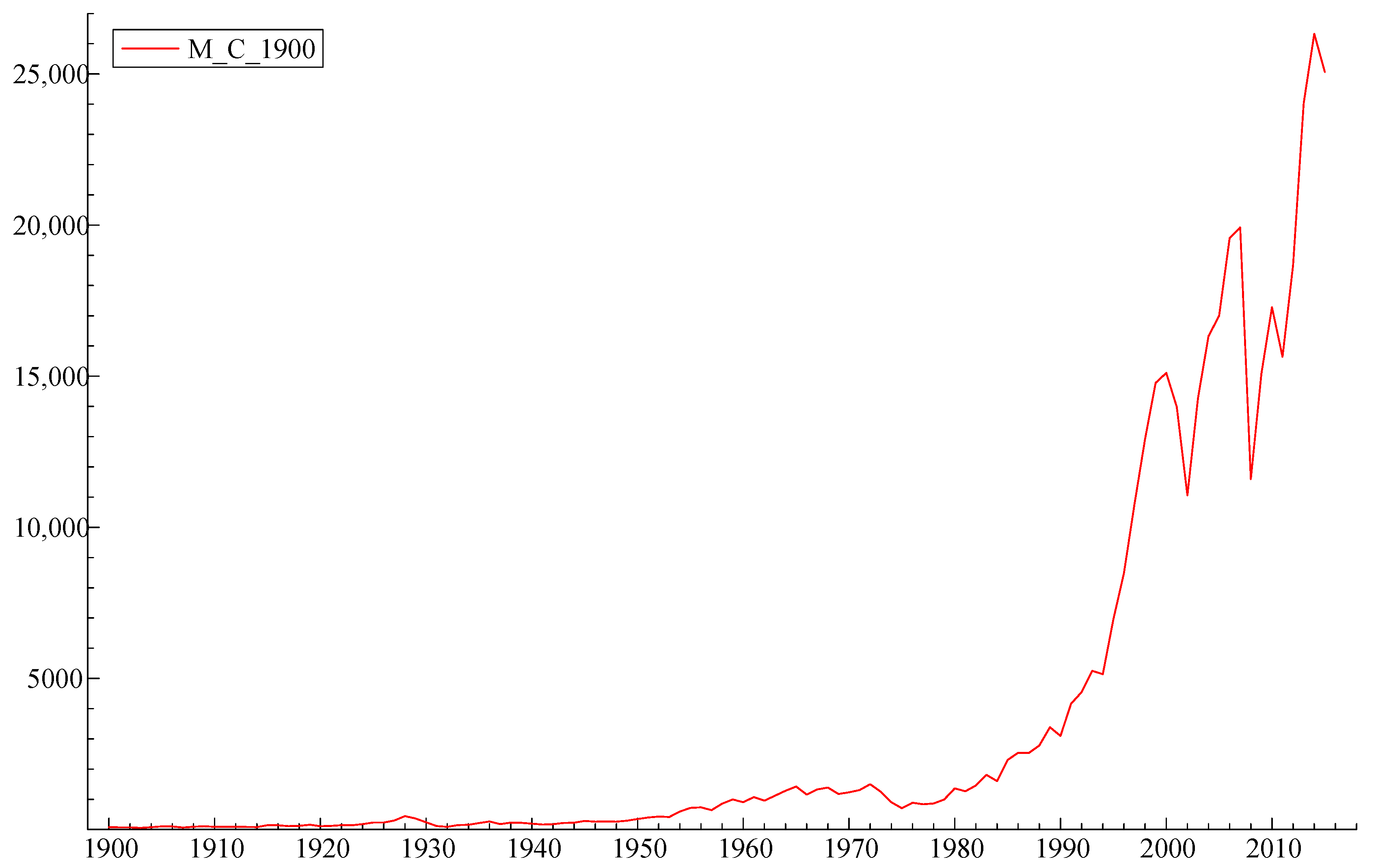
Figure 1 shows that net stockholder equity has increased very dramatically since 1980, after a major decline attributable to the dramatic oil price increase by OPEC in 1973–1974. Before that time, stock prices did not far exceed book value for most firms because financing was largely by bank loans and equity (the difference between market value and debt) was essentially a measure of current corporate profitability.

Since then, the link has been broken, thanks to several changes in the financial world. The closing of the “gold window” by President Nixon in 1971 was followed by the creation of new financial securities by securitization of mortgages in the 1970s [4]. The rise of monetarism as a financial doctrine was influential [37], as was the increasing role of the Bank of International Settlements (BIS) in Basel. The increasing role of banks as credit creators (not just transaction facilitators) is also a significant part of the story [38,39,40]. Another was the massive shift of money from investment in bonds during the inflationary years into the stock market when interest rates fell dramatically after 1982. In addition, the invention of leveraged buyouts (LBOs), corporate raiders and Michael Milken’s “junk bonds” contributed to the disconnect between profitability and market prices [4]. However, the first phase of the LBO boom ended with a crash on 19 October 1987 when the NYSE lost 554 points (22% of total value) in a day [4].

Hereafter we consider only the financial or monetizable forms of wealth. At the macroeconomic level, it is sometimes approximated by equating monetary value with cost (investment), less depreciation. This allows no net monetary benefit for the services provided, e.g., by roads and bridges, harbours, public buildings and so on. It also values services provided by the post office, public health, public schools, police, judiciary, army, and so on, at cost. The cost of these public government-provided services varies from country to country, being close to 50% of total national income in Scandinavian countries, and around 40% in the rest of Europe, but nearer 30% in the US. Yet this method of valuation seriously underestimates national wealth since it fails to reflect the fact that when the same services are provided privately (e.g., by private schools, private universities, private delivery services or private security firms), the costs, and presumably the value, of those services are far higher.

Piketty and his colleagues divide wealth into three main categories: public, non-profit and private, and within each of them, three sub-categories, viz. debt, financial assets and non-financial assets [33]. Here it is important to note that all kinds of debt instruments are also assets to lenders. Around 2.5% of US government debt (in the form of treasury bonds or T-bills) is now owned by foreign governments, especially China, Japan and the oil-exporting countries of the Persian Gulf. This is a consequence of many years of negative US trade balances.

Except for government bonds owned by foreigners, bonds represent transfers of income: current and future budgetary obligations of the US government are income-producing assets for pension funds, the US Social Security fund, insurance companies and university endowments. Similarly, corporate debt (bonds and commercial paper) are liabilities for the issuing corporations and assets to pension funds and banks. Finally, mortgages are liabilities to home owners (and other real estate owners) but assets to long-term investors. Within the US, all of these securities are simultaneously both liabilities and assets, with no net contribution to national wealth. It seems likely that US private debt held by foreigners is roughly balanced or exceeded by foreign debt held by US banks and other institutions.

Because bonds are simultaneously both assets and liabilities, they cancel out to zero except for the liabilities owed to foreign governments. Bearing in mind the above caveats, it appears that national wealth consists primarily of two major financial components, plus a few non-financial items. The first financial component of US national wealth is net stockholder equity, while the second one is net home (real estate) equity. In both cases, net equity is the surplus value after allowing for corporate debt and mortgage debt.

Non-financial but monetizable wealth consists of sole proprietorships, certificates of ownership of unincorporated small businesses, farms, shares in partnerships or closely-held corporations, copyrights on intellectual property, and marketable material assets. Financial wealth is exchangeable in markets where intermediaries (brokers) collect and match offers to buy and offers to sell at openly published prices. Non-financial wealth can be exchanged (bought and sold) privately, but only on the basis of direct negotiations between buyers and sellers.

Having noted that debts are also assets, it is important to note that the correspondence is imperfect because debts can be (and are) sometimes wiped out or converted to equity shares by defaults when borrowers cannot repay. This rarely happens to sovereign debt now, but it has happened in the past (e.g., when Russian debt was repudiated by the Bolsheviks in 1917 and German reparations debt was repudiated by the Nazi government in 1933).

When a modern country is unable to pay its debts to another country, it has to go to the International Monetary Fund (IMF), created by the Bretton–Woods agreement in 1945, which then provides new “bailout” loans. These loans are conditioned on “restructuring” the economy, usually by cutting social costs, eliminating subsidies and increasing taxes. This scenario has been implemented recently in Greece, Thailand, South Korea and Indonesia in the 1990s and several Latin American countries in the early 1980s. When non-government entities and individuals go bankrupt in the US, a judge may wipe out the unpayable debt and the creditor loses its asset. However, the bankrupt borrower loses its credit rating, often with very severe consequences: e.g., no credit cards, no checking account, rents and other purchases payable in cash in advance.

On the other hand, sovereign and corporate bonds and gold are also usable by banks as collateral for loans to third parties. Such loans carry higher interest rates thanks to higher perceived risk. In other words, borrowed money can be used as collateral for further borrowing or stock-purchasing, creating leverage “pyramids” supported by a relatively fixed pool of real assets. Bank deposits are still highly leveraged on their underlying “fractional reserves”, albeit much less than before 2008. This means that long-term bank loans still greatly exceed short-term bank deposits at any given time, so risk-free “fractional reserves”—called bank capital—are crucial.

One of the historical causes of financial crises is that many depositors, based on rumours of bank insolvency, may want their money at the same time, causing a “run on the bank”. This is what happened in the summer of 1929 when some banks had gambled too much of their depositors’ money on the rising stock market. Whenever depositors “smell” a possible problem, they may rush to withdraw their money, causing the bank failure, unless the government, or a larger bank, steps in with a “bailout”. This sort of collapse happened in various locations in the US and Europe numerous times during the 19th century and the early 20th century. The bank collapse in the US starting in 1929 was nationwide.

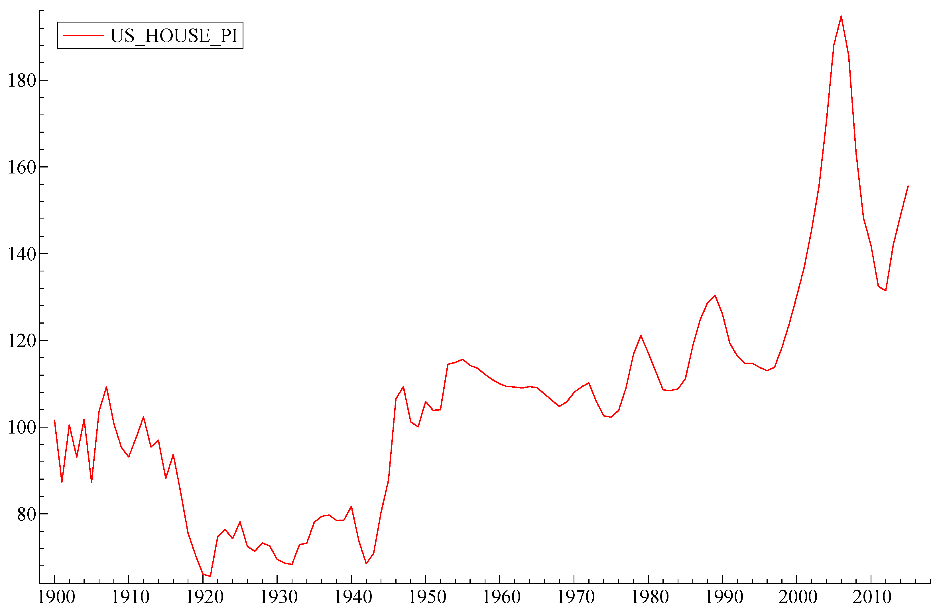
Figure 2, below, shows the Shiller house price index since 1900. Ups and downs in earlier years after WW II reflect demographic trends, e.g., the “baby boom”, and changing interest rates. Interest rates rose steadily during the 1960s and 1970s, due at first to increasing federal budget deficits caused by the Vietnam war, and later due to “inflationary expectations”. The latter ended in 1981–1982 when the FRB raised short-term interest rates to more than 20% p.a. This did kill inflationary expectations and brought US interest rates back down to earlier levels. That, in turn, sharply reduced the cost of 30-year mortgages for houses, which set off a construction boom.

The worst example of a crisis occurred in 2008 when the capital assets of many US and foreign banks included bundles of mortgage-based bonds, known as “collateralized debt obligations” or CDOs. Rather suddenly, it became evident that some of those CDOs might be worthless, or at least unsalable [41]. Since the individual mortgages included within these CDOs were “invisible” to the buyers, nobody knew which ones were safe and which ones were in danger of default. When national default rates rose above the assumed level, the CDOs all became non-marketable and illiquid overnight. It then became clear that the underlying assumption, upon which their “investment grade” AAA or AA ratings were based, was false. The underlying assumption, by FRB Chairman Greenspan and many others, was that home prices would never go down all over the country at the same time and that the rate of failure by home owners would never exceed a couple of percent or so [4].

In the fall of 2008, almost overnight, the banks and their depositors found that the banks’ capital reserves, which are supposed to be liquid, were worth much less than had been previously assumed. This initiated a ripple effect that nearly destroyed the global financial system. Banks stopped lending to each other and to other clients. Insurance companies, notably American International Group (AIG) that had insured a lot of the CDOs by selling derivatives called “credit default swaps” or CDSs, suddenly owed vast sums of money they did not have. House prices started dropping rapidly as demand dried up. Construction stopped and construction workers were laid off. The bank shares plummeted in value; one major bank, Lehman Brothers, collapsed. The consequence was a major recession that would have been much worse without the government bailouts (TARP) that came to the rescue.

The sharp decline in 2001 (the dot-com bust) and the similar decline in 2008 due to the sub-prime mortgage bust have both been followed by a long boom driven by cheap money from the FRB. Much of the cheap money provided by the Fed in 2002–2006 financed a real estate bubble in high-growth areas, especially California and Florida, which led to the financial collapse of 2008. Much of the cheap money provided by the FRB since 2009 has been diverted to private equity, hedge funds and stock buy-backs.

4. Mechanisms of Wealth Creation and Destruction

Major changes in national wealth are of several kinds. Increases are mainly due to resource discoveries, major inventions or economic growth. The major growth drivers during the first half of the 20th century were motor vehicles, electrification, farm mechanization (resulting in a massive shift of farm workers into city factories), telephones and radio. After WW II, motorization spun off secondary applications (highways, truck transport, shopping malls, air transport, tourism) while electrification continued within homes (washing machines, refrigerators, vacuum cleaners, microwave ovens, freezers, TV). Starting from wartime needs, electronic computers combined with telecommunications to create a raft of new products and industries from mainframe computers to laptops and tablets, communication satellites, bar-code readers, ATMs and digital cameras, airline scheduling, online banking, language translation, geological prospecting, word processors, browsers and search engines, smartphones, drones and the internet.

However, while these products and industries have created a great deal of wealth, they have also displaced a great many “skilled” job categories, from fitters and assemblers in factories to elevator operators and bank tellers to stenographers, typists, file clerks, law clerks and many more. Some new jobs in computer technology command higher pay, but many others (such as hotel cleaners, security guards and fast-food restaurant workers do not pay a living wage). Wealth destruction may occur as a result of technological change (e.g., automation) or physical destruction (fires, floods, earthquakes or wars).

Major wealth losses in the past may have been due to wars. Bubbles are an old story [42]. Financial collapses in the past century have resulted from the collapse of asset bubbles created by investment banks and hedge funds, with other people’s money, using excessive leverage [4]. These losses are externalities insofar as they hurt millions of people who were not involved in the activities that created the bubble. An externality is always characterized by the creation of benefits, damages or risks that are not traded in the market and that do not have market prices. We focus here especially on the latter category of losses.

At the same time, there was a major change in tax policy, as well as a growth spurt during those years, attributed by Republicans to “Reaganomics”. The obvious reasons for this growth include declining interest rates (after Paul Volcker’s “inflation killer” of 21.5% in 1981), plus a steady decline in oil prices. Reagan’s contribution was tax cuts for the rich (top income tax rates were cut from 70% to 28%, while corporate tax rates went down from 50% to 38%. However, the trade deficit also grew sharply. The immediate cause of the stock market crash of 1987 was probably a comment by the Secretary of the Treasury, James Baker, that the US dollar needed to fall (because of the trade deficit) and a bill approved by the Ways and Means Committee of the House of Representatives to disallow interest deductions on borrowing for the purpose of corporate takeovers and LBOs [4] The proposed disallowance was reversed, and the stock market recovered quickly. That “blip” scarcely shows on the chart below. Much bigger and more painful declines came later, in 1990 and 2008.

Changes in national wealth occur whenever the various asset stocks—both monetary and material—change. In a year, there may be significant absolute changes in the physical capital stock, the labour supply, or the money supply (defined broadly, to include stocks, bonds and other financial instruments). However, during an economic transaction period (minutes or hours, or a few days), those variables are relatively constant. What can (and does) change—sometimes dramatically—during shorter time periods are commodity prices, share prices, interest rates and currency exchange rates. These, in turn, can affect monetary assets and money flows, especially into (and out of) various types of investment.

The essential point of the above paragraphs is that, while material stocks do not change rapidly, money stocks and obligations, especially of margin loans and derivatives such as CDOs and CDSs, can change very rapidly. This is ultimately due to leverage, which multiplies small ripples into giant waves. Financial collapses and degrowth episodes occur when the availability of active money (available for speculative financial investments) approaches too closely to liquid reserves (i.e., the ratio approaches unity). The avalanche of selling becomes self-propelled once it starts, and momentum tends to keep it going too far (below the realistic value). The analogy with avalanches of snow on mountain slopes is obvious, but the nature of the “trigger” and the nature of the braking mechanism are not so well understood. However, after the avalanche, risk appetite declines, and real investment slows down.

When liquid financial reserves are significantly larger than short-term debts, the holders of active money are more prepared to borrow and spend it, and the economy is free to grow as fast as the stocks of capital goods, labour supply and exergy flows allow. There are several measures of financial risk that might be used, but one is the total of bank loans collateralized by stock prices and used for speculative purposes. This measure, margin debt, is compiled by the New York Stock Exchange (NYSE). It tends to correlates quite well with the economic growth rate: when the growth rate increases, margin debt increases sharply and conversely. The link to wealth creation and destruction is obvious.

5. Methodology

We have chosen to construct a dynamic multivariate econometric model that combines elements of long-term and short-term dynamics as this approach seems most suited to address the changes in wealth that took place over the chosen period of 1914–2015. We have used the advanced OxMetrics software package developed at Oxford University for estimating the coefficients in our model. The model consists of two submodels, one describing the long-term changes and the second one—the short-term fluctuations. The two subsidiary models were then re-integrated into a single overall model. We were estimating a model expressed in the following way in the general case:

W = α × X^β × Y^γ × Z^δ

(1)

which naturally led to the log-linear specification:

LogW = α + β logX + γ logY + δ logZ.

(2)

The wealth function, due to its exponential form, was modelled in logarithms, which allowed us to use a linear model. The data we have used for the econometric modelling was obtained from the Federal Reserve Bank of St Louis.

Analysis of the time series variables for the 1914–2015 model using the Augmented Dickey–Fuller (ADF) test revealed that, on the one hand, the difference in Log WEALTH (p-value < 0.0001), the change in US house price index (p-value < 0.0001), the change in Log Market Capitalization (p-value < 0.0001), the change in debt-to-GDP ratio (p-value = 0.009), the change in oil price expressed in 2015 USD (p-value = 0.038) and the change in birth and death rates spread (p-value = 0.006) were found to be stationary, as their p-values were smaller than the confidence level. On the other hand, the inflation time series was found to be non-stationary (p-value = 0.055) and unemployment was found to be non-stationary too, as the p-value is equal to 0.190, which is greater than the confidence level (0.05). It should be noted that if the Log Wealth _t−1 member is transferred to the left-hand side of the main equation, the left-hand side turns into the change in Log WEALTH and becomes stationary.

6. Results

Table 1. Statistical coefficients of the short-run difference model of US wealth (1914–2015).

	Coefficient	Std. Error	t-Value	t-Prob	Part. R2
Change in Log WEALTH t−2	−0.255749	0.06130	−4.17	0.0001	0.1667
Change in Log WEALTH t−4	−0.125872	0.05589	−2.25	0.0268	0.0551
Constant	0.0373512	0.01056	3.54	0.0007	0.1257
Unemployment t−1	−0.00200153	0.0007172	−2.79	0.0065	0.0822
Inflation	−0.00354843	0.0006925	−5.12	0.0000	0.2318
Change in US House Price Index	0.00284287	0.0005107	5.57	0.0000	0.2626
Change in Log Market Capitalization	0.141734	0.01377	10.3	0.0000	0.5492
Change in Log Market Capitalization t−1	0.0766456	0.01466	5.23	0.0000	0.2390
Change in Debt-to-GDP Ratio t−1	−0.00113039	0.0005257	−2.15	0.0343	0.0505
Glass–Steagall Act t−1	0.0174061	0.006448	2.70	0.0083	0.0773
Change in Log M2 t−2	0.129906	0.05508	2.36	0.0206	0.0601
Federal 10-Year Bond Yield t−2	−0.00873970	0.003989	−2.19	0.0311	0.0523
Federal 10-Year Bond Yield t−3	0.00860895	0.004000	2.15	0.0341	0.0506
Change in Oil Price Expressed in 2015 USD t−1	0.000757646	0.0002976	2.55	0.0127	0.0693
Change in Birth and Death Rate Spread	−0.00545968	0.002852	−1.91	0.0589	0.0404

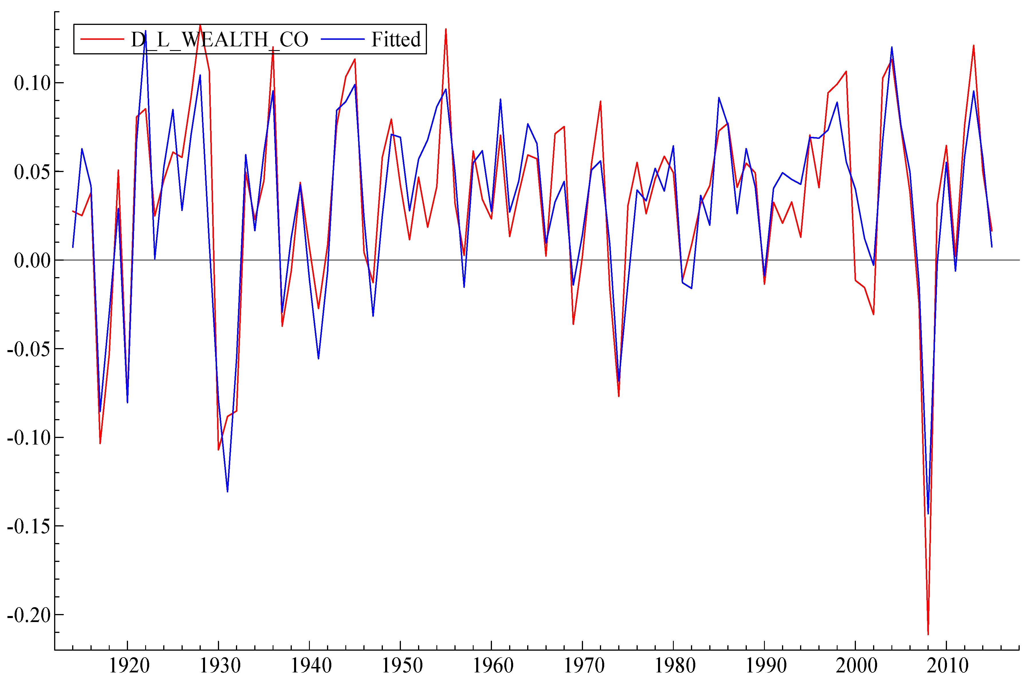
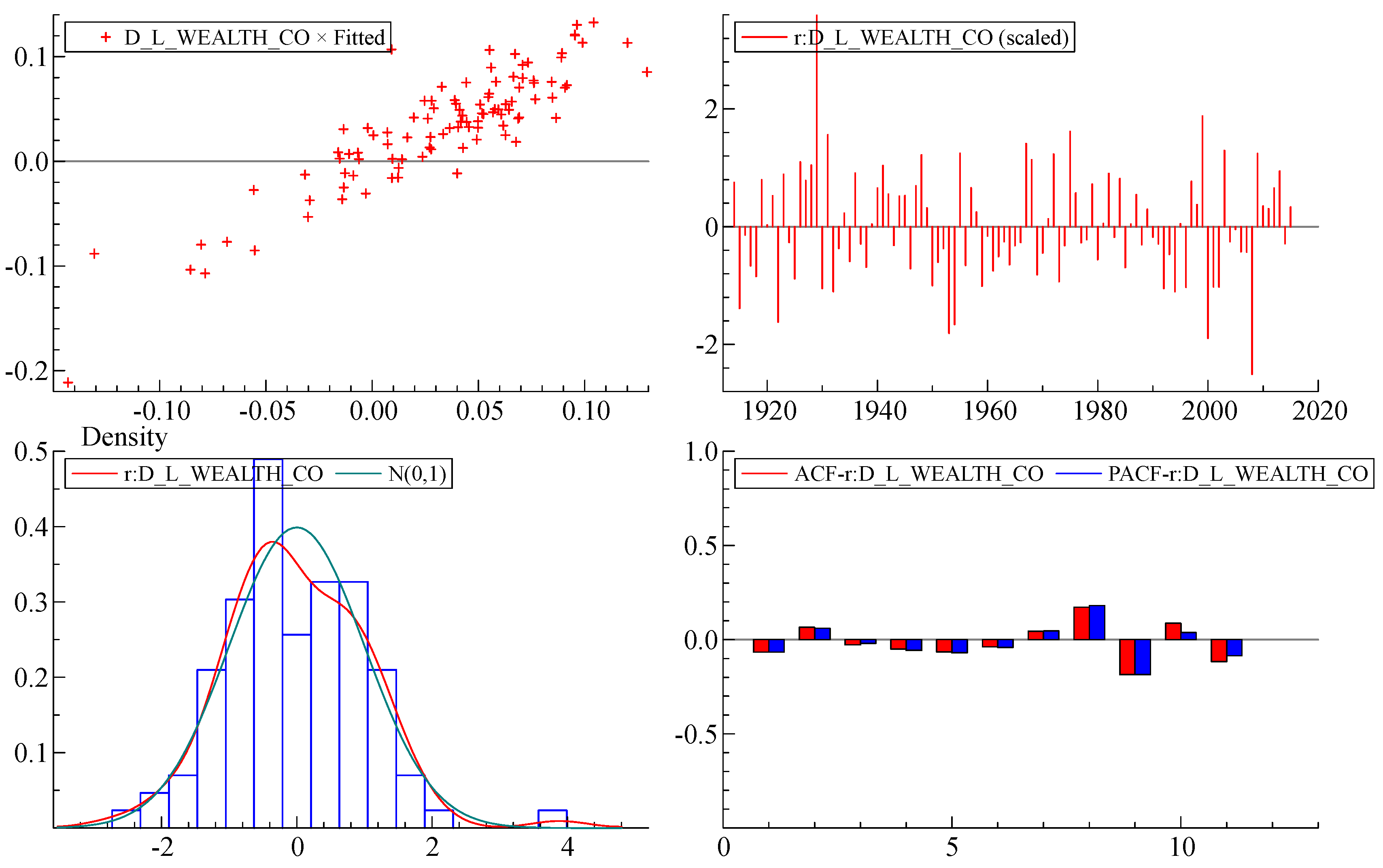
Source: Author calculations. The R² for this model is 0.797169. Red colour denotes t-probabilities < 0.05.

lists the variables of the short-term submodel, all of which are constrained to lie in the range (roughly) plus or minus 0.1. The letter D means that the variable is a year-to-year difference. The letter L indicates that the model variable is a natural logarithm. First, we estimated the model (Figure 3) in difference form. 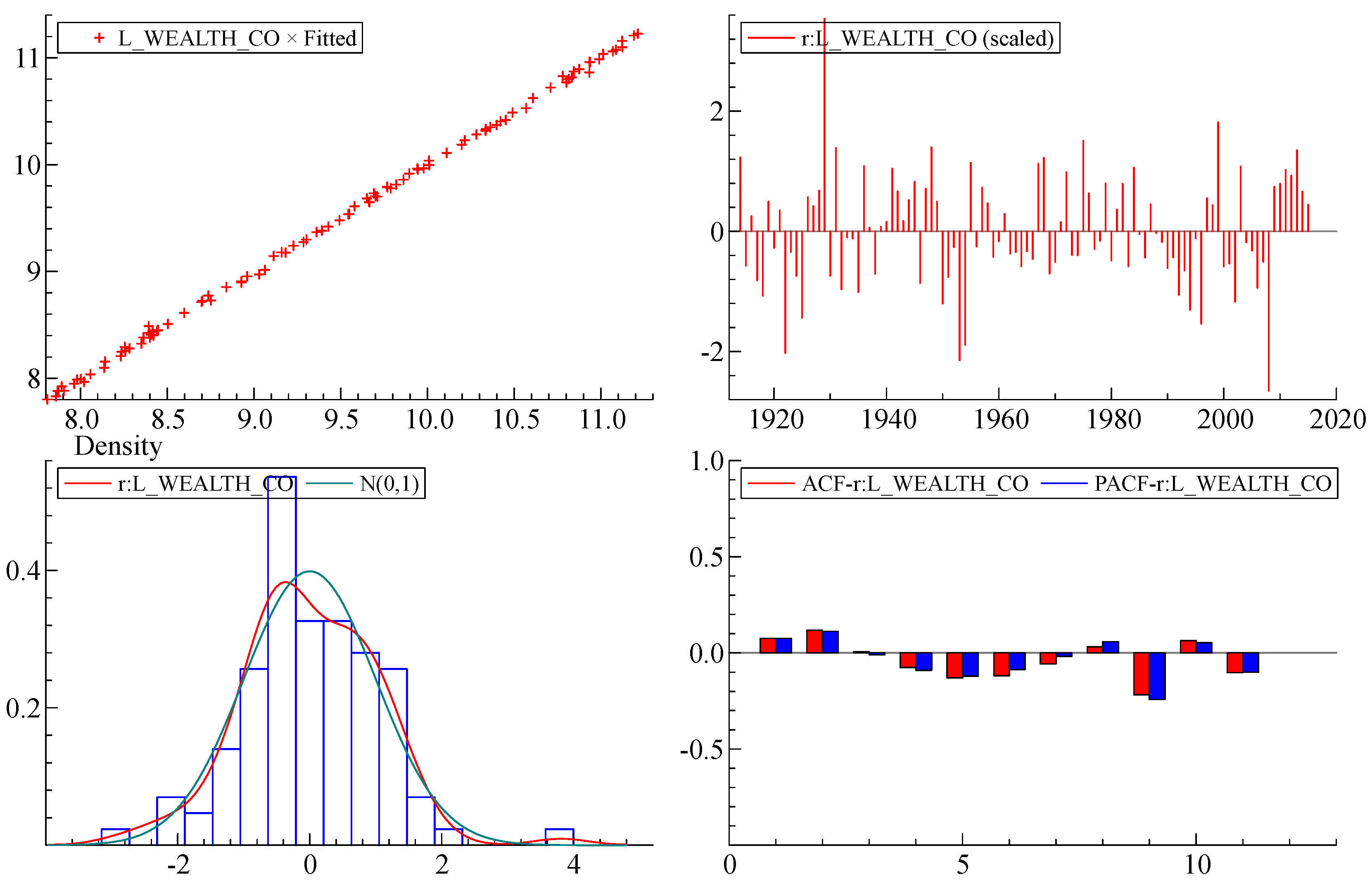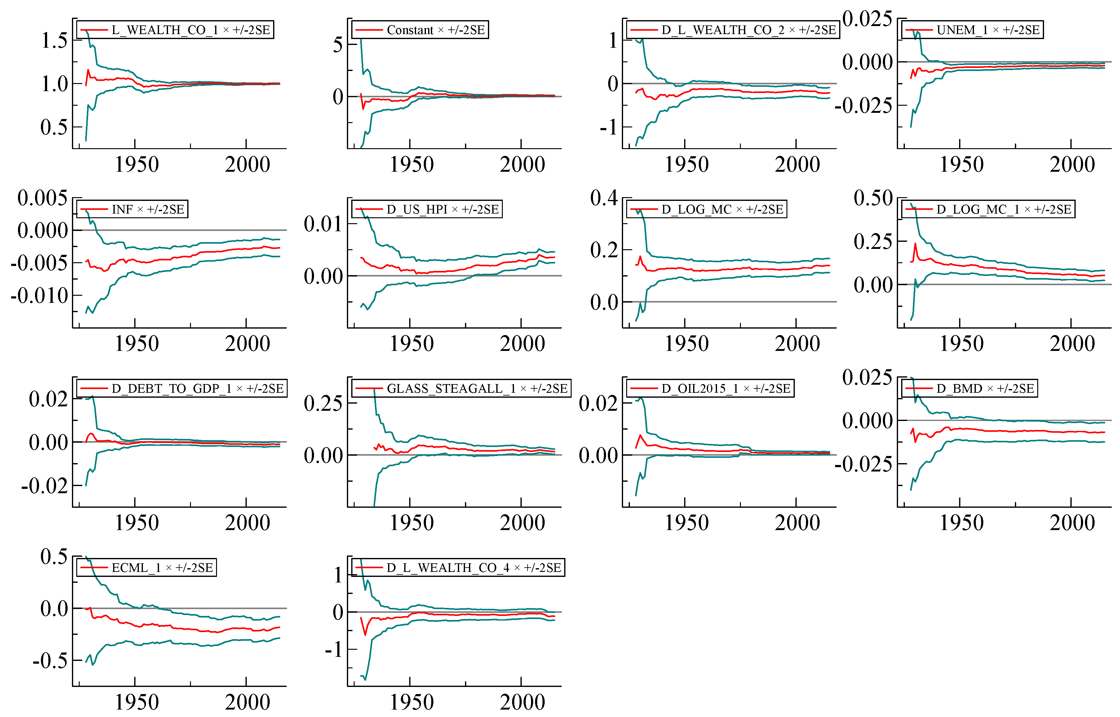We found a functional form that explained a significant proportion in the variation of the dependent variable (R² = 0.79). Most standard model specification tests have been met: there is no autocorrelation and no heteroscedasticity in the residuals, with a slight deviation from the strict normality of the error distribution. The coefficients in the model are shown to be very stable. (See Figure A2 in Appendix A).

The White heteroscedasticity test [43] is designed to establish whether the residual variance of a variable in a regression model is constant. This test gives F(27,74) = 0.91845 with a significance of 0.5850. This means that the probability of an F-statistic being greater than or equal to the observed value is higher than the 0.05 level, and therefore the null hypothesis of homoscedasticity cannot be rejected.

The Ramsey regression equation specification error test (RESET23) tests specification in the form of a null hypothesis that a₁ = a₂ = a₃ = 0 in the

Y_i = a₀ + a₁X_i + a₂Ŷ_i2 + a₃Ŷ_i3 + v_i, i = 1, 2, ..., n,

(3)

where Ŷ_i denotes the fitted values [44]. The null hypothesis in the short-run model cannot be rejected at 1% significance level or less, so the model specification is quite good.

Residual autocorrelation AR 1–2 test is a standard test of autocorrelation up to degree 2 with F(2,85) = 0.48087 [0.6199] [45]. The null hypothesis is a₁ = a₂ = 0 in an auxiliary regression: ê_t = a₀ + a₁ê_t−1 + a₂ê_t−2 + a₃X_t + v_t. The probability of a value of F greater or equal to the observed value is [0.6199], which is higher than the significance level of 5%; therefore, the null hypothesis cannot be rejected, which means there is no residual autocorrelation. This is confirmed by the visual analysis of the autocorrelation function for residuals in Appendix A.

Autoregressive Conditional Heteroscedasticity was assessed through the ARCH test [46]. The null hypothesis of constant variance cannot be rejected according to the ARCH criterion 1.0233 [0.3142]. In this instance, we can conclude that the short-run model design is reasonable.

The distribution of the residuals (errors) in the short-run model differs slightly from strict normality.

We then estimated the long-run equation in levels of the logarithms of wealth (Log WEALTH) and used a static long-run solution to generate an error correction term. The resulting model combined the elements of the long-term and short-term effects. It is interesting to note that the oil price and unemployment only mattered for the short-term adjustments, and money supply M2 was significant only in the long-run equation.

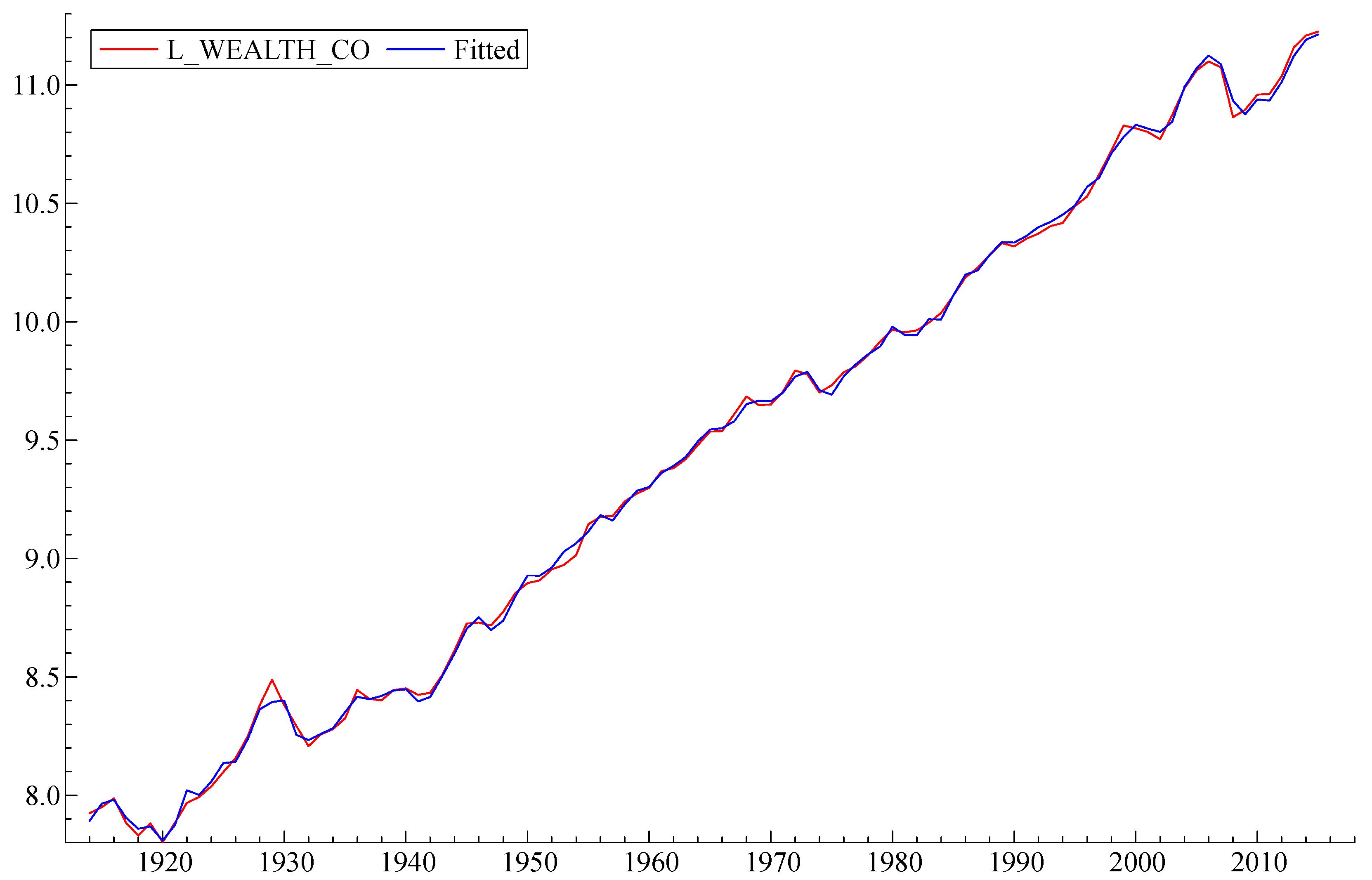
The next step is to integrate the logarithmic functions and the differentials to form the final version of the model. The result (in logarithms) is shown in Figure 4 below. The variables of the final model are listed in

Table 2. Statistical coefficients of the final aggregated model of US wealth (1914–2014).

	Coefficient	Std. Error	t-Value	t-Prob	Part. R2 L_
Constant	0.0583078	0.02642	2.21	0.0299	0.0524
Log WEALTH t−1	0.998494	0.002663	375.	0.0000	0.9994
Change in Log WEALTH t−2	−0.214622	0.05958	−3.60	0.0005	0.1285
Change in Log WEALTH t−4	−0.112620	0.05475	−2.06	0.0426	0.0459
Change in Log Market Capitalization	0.139638	0.01339	10.4	0.0000	0.5528
Change in Log Market Capitalization t−1	0.0517058	0.01430	3.61	0.0005	0.1293
Change in US House Price Index	0.00356172	0.0005145	6.92	0.0000	0.3526
Inflation	−0.00271266	0.0006502	−4.17	0.0001	0.1651
Unemployment t−1	−0.00225701	0.0006420	−3.52	0.0007	0.1231
Glass–Steagall Act t−1	0.0165057	0.006056	2.73	0.0077	0.0778
Change in Birth and Death Rate Spread	−0.00684823	0.002778	−2.47	0.0156	0.0646
Change in Oil Price Expressed in 2015 USD t−1	0.000698445	0.0002858	2.44	0.0165	0.0636
Change in Debt-to-GDP Ratio t−1	−0.00103389	0.0005048	−2.05	0.0435	0.0455
Error Correction Term	−0.182980	0.05141	−3.56	0.0006	0.1258

Source: Author calculations. Red colour denotes t-probabilities < 0.05.

.

Note that the model reproduces both the overall growth and essentially all of the major wealth fluctuations of the US economy during those years. It correctly “predicts” or reproduces the 1920s boom, the crash of 1929 followed by the great depression, the post-WW II “baby boom” the recession after the OPEC oil price increases in 1973–1974, the “dot-com” crash of 2000, and the sub-prime mortgage crash of 2008.

The final model produced a very good fit with R² = 0.99943. The Log WEALTH has a significant positive autocorrelation term expressed by its first lag and two lagged negative terms of first differences of Log WEALTH: Change in Log WEALTH _t−2 and Change in Log WEALTH _t−4 (second and fourth lag). Log WEALTH is also dependent on the first lag of the unemployment rate (Unemployment _t−1), which is featured here with a negative coefficient. The rate of inflation (Inflation) features significantly with a negative coefficient. Log WEALTH is related to the first difference of US house price index (Change in US House Price Index) and the first difference of the logarithm of (stock) market capitalization in the US economy (Change in Log Market Capitalization) as well as its first lag (Change in Log Market Capitalization _t−1), all with positive coefficients. The dependent variable is also related to the lagged first difference in the debt-to-GDP ratio (Change in Debt-to-GDP Ratio _t−1) with a negative coefficient and positively related to the lagged first difference in the oil price, expressed in 2015 US dollars (Change in Oil Price Expressed in 2015 USD _t−1). There is a significant component related to the first differences in the spread between birth rates and death rates in the US (Change in Birth and Death Rate Spread) and the variable representing the Glass–Steagall Act, which prohibited commercial banks from speculative activity in the stock market after 1933. This has also been found to be significant for explaining the total US wealth.

In other words, the total wealth tended to grow with its past values, the US house prices, the market capitalization of US companies, when Glass–Steagall Act was in place and when changes in the oil price were higher. The total wealth tended to diminish if its growth 2 and 4 periods ago was high, when unemployment increased in the previous period and high inflation was observed in the current period, with the growth in changes in the debt-to-GDP ratio and increases in the difference between births and deaths in the US.

The value of the Akaike information criterion for the final model we observed was −7.13023, which is a considerable improvement on the long-run equation. The final model exhibits no autocorrelation or heteroscedasticity in the residuals and no issues with the model specification, judged by the RESET test. It still deviates slightly from strict normality in the distribution of the residuals.

The White heteroscedasticity test [43] is designed to establish whether the residual variance of a variable in a regression model is constant. The test shows that with a significance level of 0.4162, the White test gives F(25,76) = 1.0524 (0.4162). This means that the probability of an F-statistic being greater than or equal to the observed value is higher than the 0.05 level, and therefore the null hypothesis of homoscedasticity cannot be rejected.

The Ramsey regression equation specification error test (RESET23) tests the validity of the model specification. The null hypothesis is that the coefficients a₁ = a₂ = a₃ = 0 in

Y_i = a₀ + a₁X_i + a₂Ŷ_i2 + a₃Ŷ_i3 + v_i, i = 1, 2, ..., n,

(4)

where Ŷ_i denotes the fitted values [44]. The null hypothesis cannot be rejected at 1% significance level or less, so the final model specification is quite good. Residual autocorrelation (AR 1-2 test) is a standard test of autocorrelation up to degree 2 with a F(2,86) = 1.6506 [0.1980] [45]. The null hypothesis is a₁ = a₂ = 0 in an auxiliary regression:

ê_t = a₀ + a₁ê_t−1 + a₂ê_t−2 + a₃X_t + v_t.

(5)

The probability of a value of F greater or equal to the observed value is [0.1980], which is higher than the significance level of 5%; therefore, the null hypothesis cannot be rejected, which means there is no residual autocorrelation in the final model, which is confirmed by the visual analysis of the autocorrelation function for residuals in Annex 2. Autoregressive Conditional Heteroscedasticity is assessed through the ARCH test [46]. The null hypothesis of constant variance cannot be rejected according to the ARCH criterion 0.062762 [0.8027], and in this instance, we conclude that the final model design is reasonable. The stability of the parameters of the final model is slightly lower than for the short-run differences model, as can be seen in Appendix B.

Judging by the partial R², the most important variable in terms of its contribution to the variance in Log WEALTH is the autocorrelation term Log WEALTH _t−1 (partial R² = 0.9994), followed by the change in Log Market Capitalization (partial R² = 0.5528) and change in US House Price Index (partial R² = 0.3526), followed by inflation (partial R² = 0.1615).

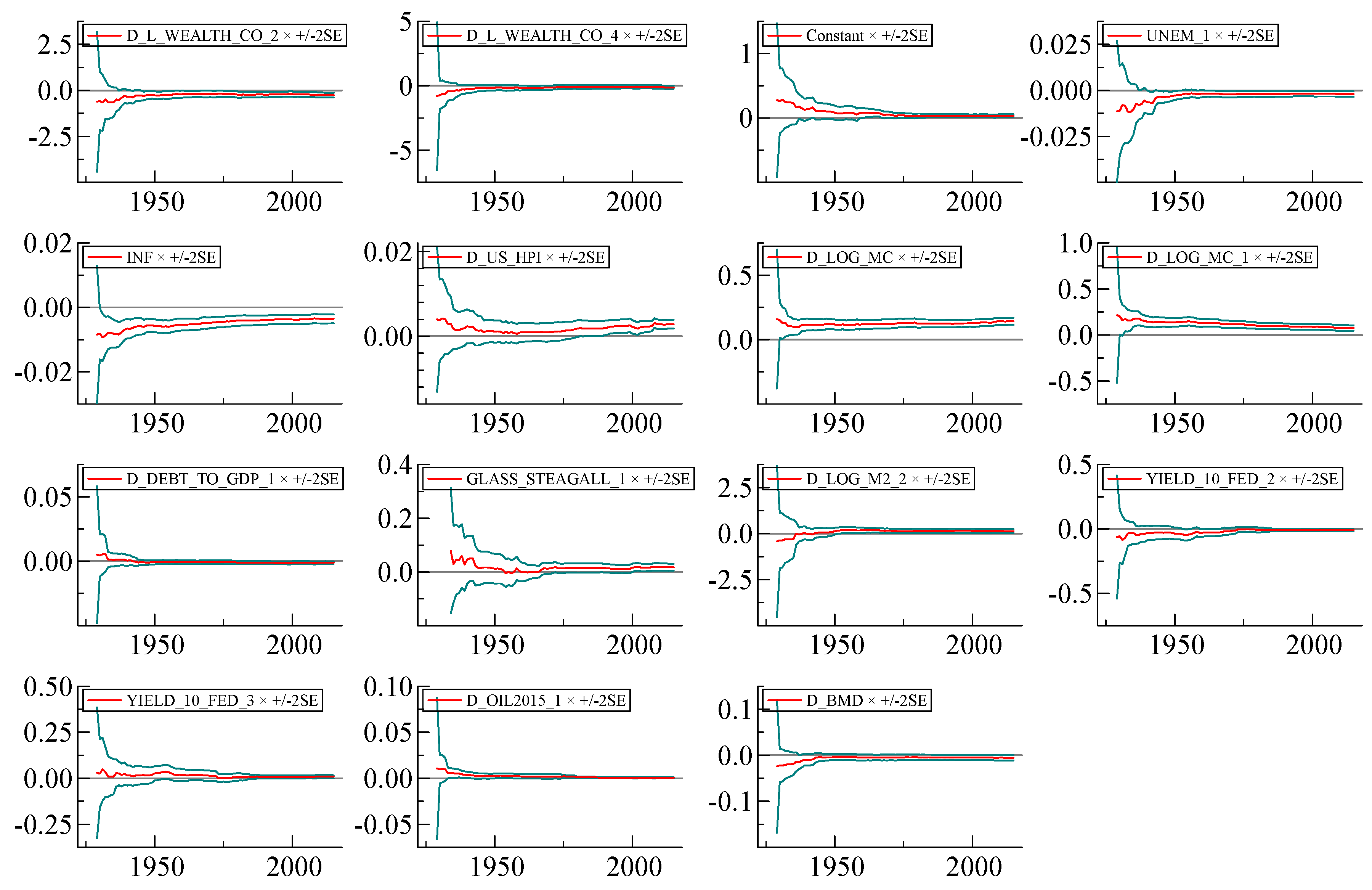
We would like to emphasize a particular strength of our model exhibited in Figure A2; it has very stable short-run coefficients over the very long term from before WWII to the present day. We have tried to make sure that the final version of the model combining the long run and the short run has the coefficients that are as stable as possible (Figure A7).

Although the time covered by the model is unique (1914–2015), covering the most recent period (2016–2021) could be the subject of our future research. Moreover, in the future, we will be aiming to bring in additional functions in the model to make it run as a simultaneous equations package.

The model described above is capable of assessing the magnitude of changes in total wealth given the changes in explanatory variables. For instance, a 1% increase in unemployment in a given year would wipe off around $1 billion off the total US wealth the next year. A 1% increase in inflation would have a similar effect.

The original question raised at the end of Section 1 was whether the middle-class financial losses in the past century were exogenous “black swans” or endemic consequences of the structure of the financial system. The remarkable accuracy of the model strongly suggests the latter. However, one-time events, such as the failure of Credit Anstalt in 1930, or the Arab oil boycott in 1972 or the failures of WorldCom and Enron in 1999, might be misconstrued (by some) as causes. (In fact, the sharp rise in oil prices in 1973 almost certainly did cause the recession that followed. For that reason, we included the price of oil as one of the variables in the model, and it is significant.)

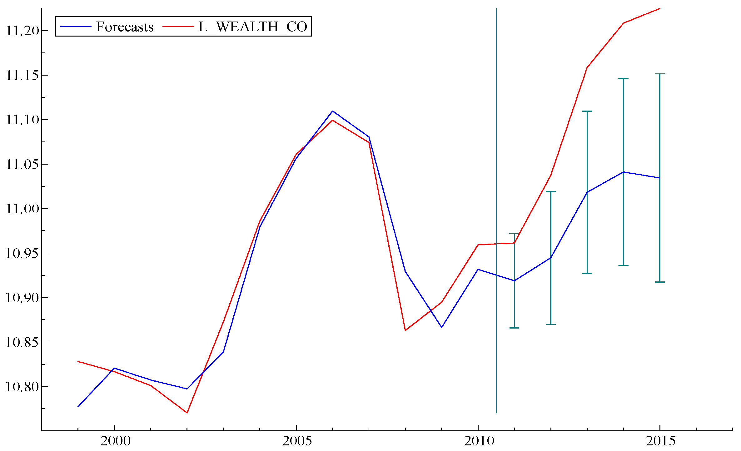
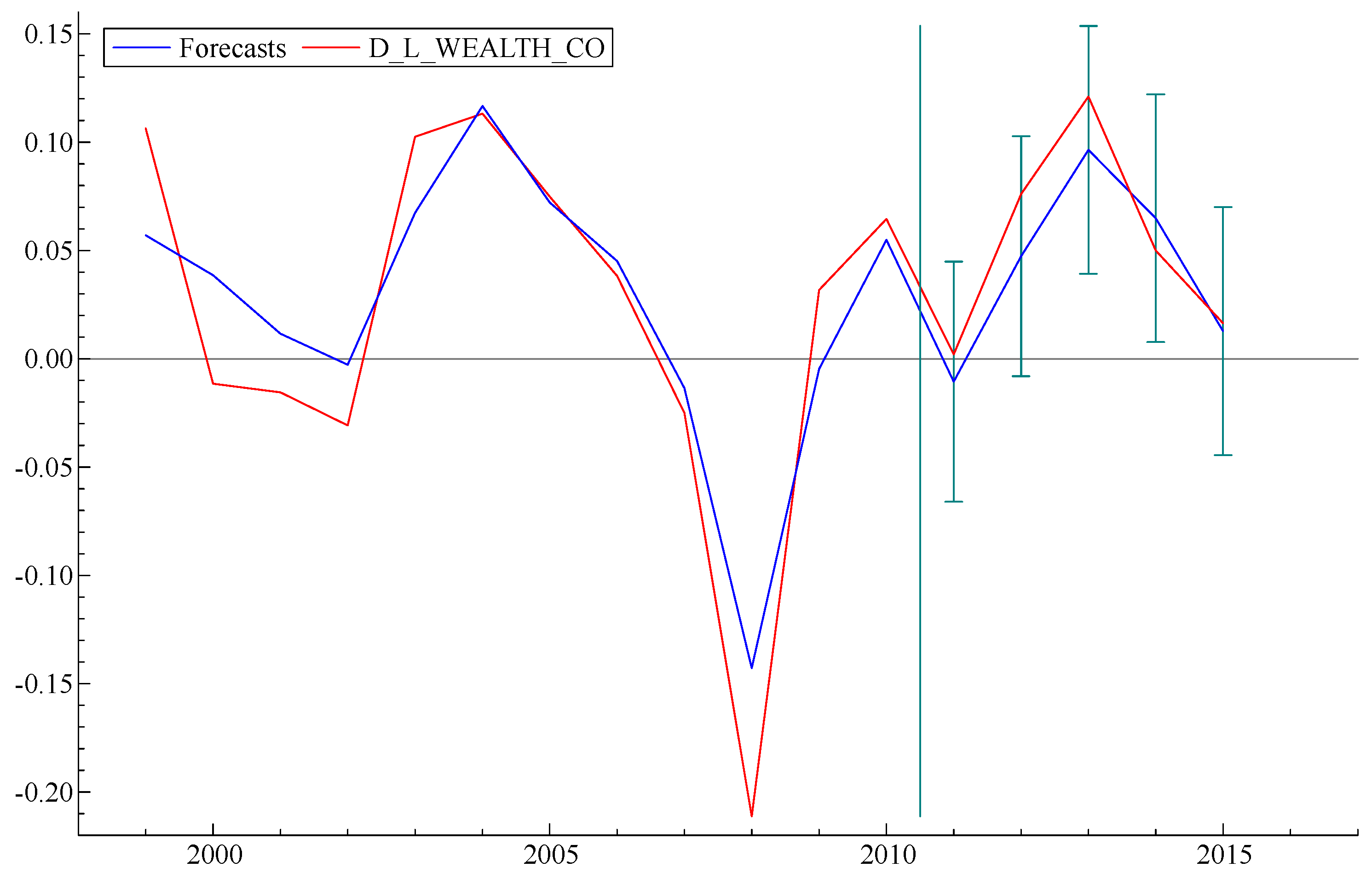
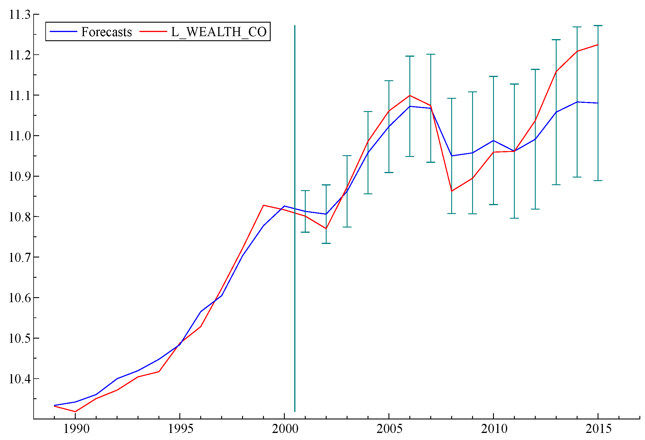
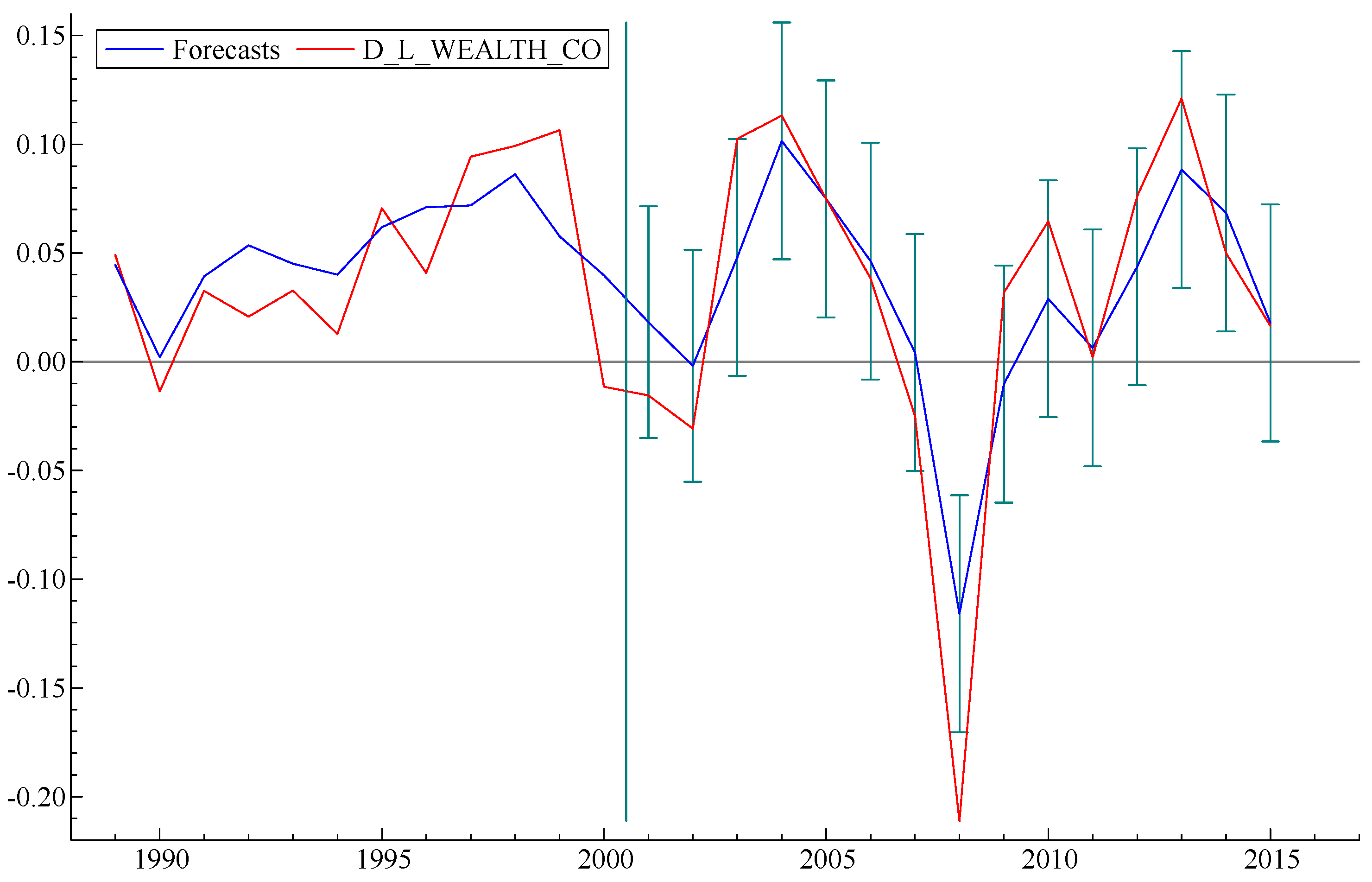
To take the argument a step further, we carried out a simple exercise, as follows: What would the model “predict” if data from recent years were excluded from the “fitting” process? Graphs of three forecasts obtained from three versions of the model, as fitted by data up to 2010, 2005 and 2000, respectively, are displayed in Figure 5, Figure 6 and Figure 7 below, with error bars. It is interesting to note that the model forecast, based on fitting data prior to 2000, predicts subsequent events—including the sharp decline starting in 2008—to an accuracy well within the error bars. Curiously, Figure 5, based on data through 2010, significantly underestimates the subsequent recovery. This strongly suggests that TARP and the later actions of the Fed, such as three stages of “quantitative easing”, which were not taken into account in the model fitting data, significantly improved the pace of the economic recovery.

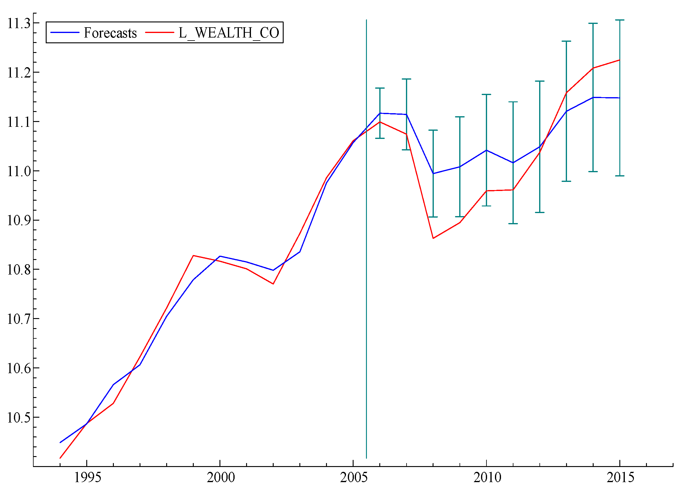
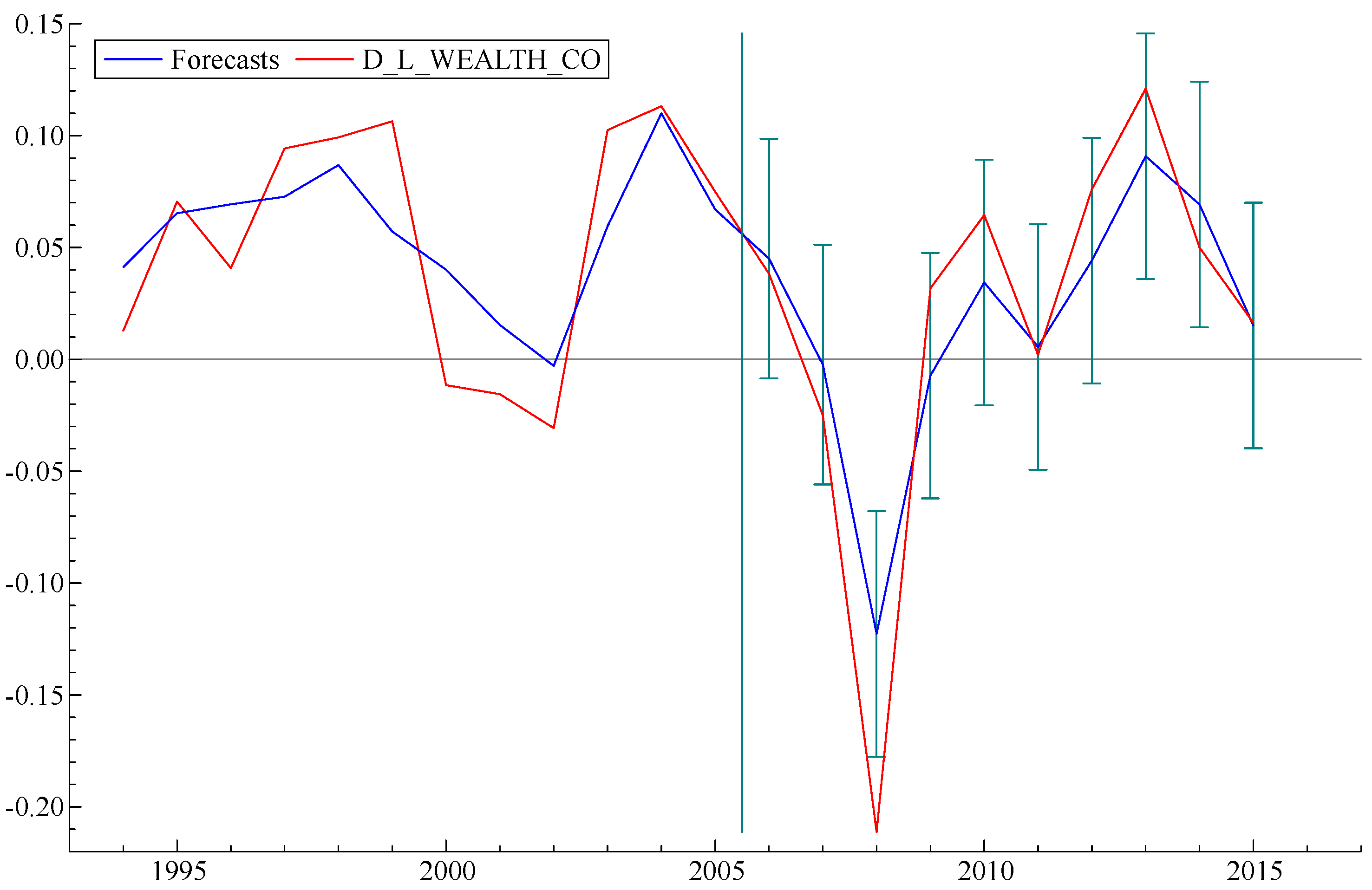
On the other hand, when the model is fitted by data only up to 2005 (Figure 6), it correctly predicts the date of the subsequent collapse in 2008 but underestimates the magnitude of the actual losses. The forecast that started in 2000 (Figure 7) got the date of the 2008 collapse correct but underestimated both the severity of the loss and the recovery.

7. Conclusions

These results suggest that whatever caused the financial collapse of 2008 was already “built in” to the financial system. The model is capable of explaining what the most critical variables are and what is the direction and the magnitude of the likely effects. Further analysis could provide clues towards how the “next” financial crisis (expected by many financial analysts) can be avoided. More research is obviously needed to answer that question. However, the results do suggest that the model may be usable for forecasting future financial instabilities with some confidence, based on extrapolations of the variables in the model. We have found that the most important factors contributing to the variation in US wealth have been: the wealth itself observed in the previous period, change in market capitalization, change in US house price index and inflation. Less impactful but statistically significant factors included unemployment, changes in oil price, and change in debt-to-GDP ratio. Another significant result is that the Glass–Steagall Act, which prohibited commercial banks from speculative activity in the stock market after 1933, had a statistically significant positive impact on wealth in the US. Our model, in the absence of data from after 2000, was able to reasonably accurately predict the 2008 financial crisis. We have found our model to be slightly more accurate in the short run than in the long run.