
Inner Damping of Water in Conduit of Hydraulic Power Plant


Abstract
1. Introduction
2. Theory
2.1. Continuity Equation
2.2. Momentum Equation
2.3. Second Viscosity
3. Measurement
4. Evaluation
5. Summary
Author Contributions
Funding
Institutional Review Board Statement
Informed Consent Statement
Data Availability Statement
Conflicts of Interest
Symbols
| a | wave speed |
| b | bulk viscosity |
| D | pipe diameter |
| E | Young’s modulus |
| e | pipe wall thickness |
| f | frequency |
| gravity acceleration projection to pipe axis | |
| i | imaginary unit |
| Bessel function | |
| Bessel function | |
| n | normal vector oriented out of liquid |
| P | pipe wall area |
| p | pressure |
| Q | flow rate |
| S | pipe cross-section |
| s | parameter of Laplace transformation |
| T | transfer matrix |
| t | time |
| V | volume |
| v | velocity |
| x | longitudinal coordinate |
| pipe wall damping | |
| deformation | |
| dynamic viscosity | |
| friction coefficient | |
| second viscosity | |
| density | |
| stress | |
| angular velocity | |
| Subscripts: | |
| c | complex number |
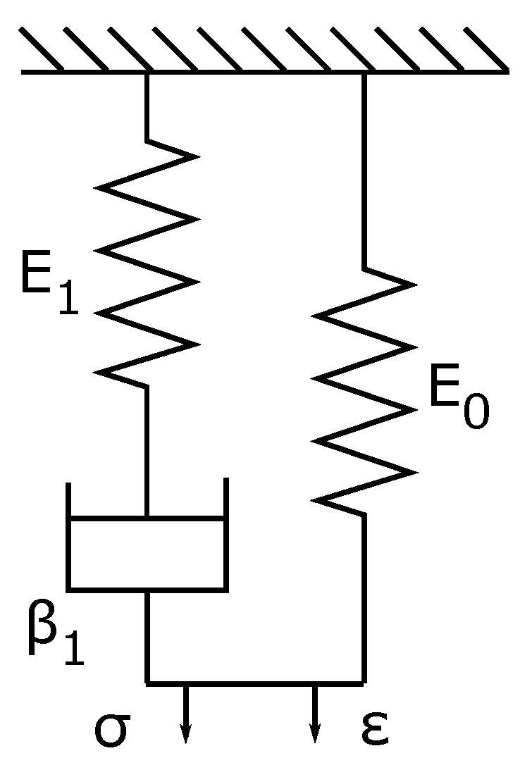
| 0 | see Figure 1 |
| 1 | see Figure 1 |
| Superscripts: | |
| * | value divided by steady value |
| variable after Laplace transformation | |
References
- Alligne, S.; Nicolet, C.; Tsujimoto, Y.; Avellan, F. Cavitation surge modelling in Francis turbine draft tube. J. Hydraul. Res. 2014, 52, 399–411. [Google Scholar] [CrossRef]
- Liu, H.; Ouyang, H.; Wu, Y.; Tian, J.; Du, Z. Investigation of unsteady flows and noise in rotor-stator interaction with adjustable lean vane. Eng. Appl. Comp. Fluid 2014, 8, 299–307. [Google Scholar] [CrossRef][Green Version]
- Vítkovský, J.P.; Bergant, A.; Simpson, A.R.; Lambert, M.F. Systematic evaluation of one-dimensional unsteady friction models in simple pipelines. J. Hydraul. Eng. 2006, 132, 696–708. [Google Scholar] [CrossRef]
- Keramat, A.; Kolahi, A.G.; Ahmadi, A. Waterhammer modelling of vicoelastic pipes with a time-dependent Poissons’s ratio. J. Fluid. Struct. 2013, 43, 164–178. [Google Scholar] [CrossRef]
- Pochylý, F.; Habán, V.; Fialová, S. Bulk viscosity—Constitutive equations. Int. Rev. Mech. Eng. 2011, 5, 1043–1051. [Google Scholar]
- Cannizzaro, D.; Pezzinga, G. Energy dissipation in transient gaseous cavitation. J. Hydraul. Eng. 2005, 131, 724–732. [Google Scholar] [CrossRef]
- Jablonská, J. Compressibility of the fluid. EPJ Web. Conf. 2014, 67, 322–327. [Google Scholar] [CrossRef]
- Graves, R.E.; Argrow, B.M. Bulk viscosity: Past to present. J. Thermophys. Heat Tr. 1999, 13, 337–342. [Google Scholar] [CrossRef]
- Dellar, P.J. Bulk and shear viscosities in lattice Boltzmann equations. Phys. Rev. E 2001, 64, 11. [Google Scholar] [CrossRef] [PubMed]
- Zuckerwar, A.J.; Ash, R.L. Volume viscosity in fluids with multiple dissipative processes. Phys. Fluids 2009, 21, 12. [Google Scholar] [CrossRef]
- Marner, F.; Scholle, M.; Herrmann, D.; Gaskell, P.H. Competing Lagrangians for incompressible and compressible viscous flow. Roy Soc. Open Sci. 2019, 6, 14. [Google Scholar] [CrossRef] [PubMed]
- Scholle, M. A discontinuous variational principle implying a non-equilibrium dispersion relation for damped acoustic waves. Wave Motion 2020, 98, 11. [Google Scholar] [CrossRef]
- Karim, S.M. Second viscosity coefficient of liquid. J. Acoust. Soc. Am. 1953, 25, 997–1002. [Google Scholar] [CrossRef]
- Dukhin, A.S.; Goetz, P.J. Bulk viscosity and compressibility measurement using acoustic spectroscopy. J. Chem. Phys. 2009, 130, 13. [Google Scholar] [CrossRef] [PubMed]
- Holmes, M.J.; Parker, N.G.; Povey, M.J.W. Temperature dependence of bulk viscosity in water using acoustic spectroscopy. J. Phys. Conf. Ser. 2011, 269, 7. [Google Scholar] [CrossRef]
- He, X.; Wei, H.; Shi, J.; Liu, J.; Li, S.; Chen, W.; Mo, X. Experimental measurement of bulk viscosity of water based on stimulated Brillouin scattering. Opt. Commun. 2012, 285, 4120–4124. [Google Scholar] [CrossRef]
- Himr, D.; Habán, V.; Fialová, S. Influence of second viscosity on pressure pulsation. Appl. Sci. 2019, 9, 5444. [Google Scholar] [CrossRef]
- Dörfler, P. Pressure wave propagation and damping in a long penstock. In Proceedings of the 4th International Meeting on Cavitation and Dynamic Problems in Hydraulic Machinery and Systems, Belgrade, Serbia, 26–28 October 2011. [Google Scholar]
- Zielke, W. Frequency-dependent friction in transient pipe flow. J. Basic Eng. 1968, 90, 109–115. [Google Scholar] [CrossRef]
- Zielke, W. Frequency Dependent Friction in Transient Pipe Flow. Ph.D. Thesis, The University of Michigan, Ann Arbor, MI, USA, 1966. [Google Scholar]
- Záruba, J. Water Hammer in Pipe-Line Systems, 2nd ed.; Academia: Prague, Czech Republic, 1993. [Google Scholar]


| Real Part (), Imaginary Part (), Frequency (f) | Shape of Pressure Amplitudes along the Conduit |
|---|---|
| = 0.0121522 rad/s = 1.403 rad/s f = 0.223 Hz |  |
| = 0.01469911 rad/s
= 4.235 rad/s f = 0.674 Hz |  |
| = 0.03323047 rad/s
= 6.991 rad/s f = 1.113 Hz |  |
| = 0.03837075 rad/s
= 9.792 rad/s f = 1.558 Hz |  |
| = 0.04869796 rad/s
= 12.610 rad/s f = 2.007 Hz |  |
| = 0.08408768 rad/s
= 15.355 rad/s f = 2.444 Hz |  |
| = 0.07548372 rad/s
= 18.156 rad/s f = 2.890 Hz |  |
Publisher’s Note: MDPI stays neutral with regard to jurisdictional claims in published maps and institutional affiliations. |
© 2021 by the authors. Licensee MDPI, Basel, Switzerland. This article is an open access article distributed under the terms and conditions of the Creative Commons Attribution (CC BY) license (https://creativecommons.org/licenses/by/4.0/).
Share and Cite
Himr, D.; Habán, V.; Štefan, D. Inner Damping of Water in Conduit of Hydraulic Power Plant. Sustainability 2021, 13, 7125. https://doi.org/10.3390/su13137125
Himr D, Habán V, Štefan D. Inner Damping of Water in Conduit of Hydraulic Power Plant. Sustainability. 2021; 13(13):7125. https://doi.org/10.3390/su13137125
Chicago/Turabian StyleHimr, Daniel, Vladimír Habán, and David Štefan. 2021. "Inner Damping of Water in Conduit of Hydraulic Power Plant" Sustainability 13, no. 13: 7125. https://doi.org/10.3390/su13137125
APA StyleHimr, D., Habán, V., & Štefan, D. (2021). Inner Damping of Water in Conduit of Hydraulic Power Plant. Sustainability, 13(13), 7125. https://doi.org/10.3390/su13137125